Performance of QUIC Implementations Over Geostationary Satellite Links

Abstract

QUIC was recently standardized as RFC 9000, but the performance of QUIC over geostationary satellite links is problematic due to the non-applicability of Performance Enhancing Proxies. As of today, there are more than a dozen of different QUIC implementations. So far performance evaluations of QUIC over satellite links were limited to specific QUIC implementations. By deploying a modified version of the IETF QUIC-Interop-Runner, this paper evaluates the performance of multiple QUIC implementations over multiple geostationary satellite links. This includes two emulated ones (with and without packet loss) and two real ones. The results show that the goodput achieved with QUIC over geostationary satellite links is very poor in general, and especially poor when there is packet loss. Some implementations fail completely and the performance of the other implementations varies greatly. The performance depends on both client and server implementation.

I Introduction

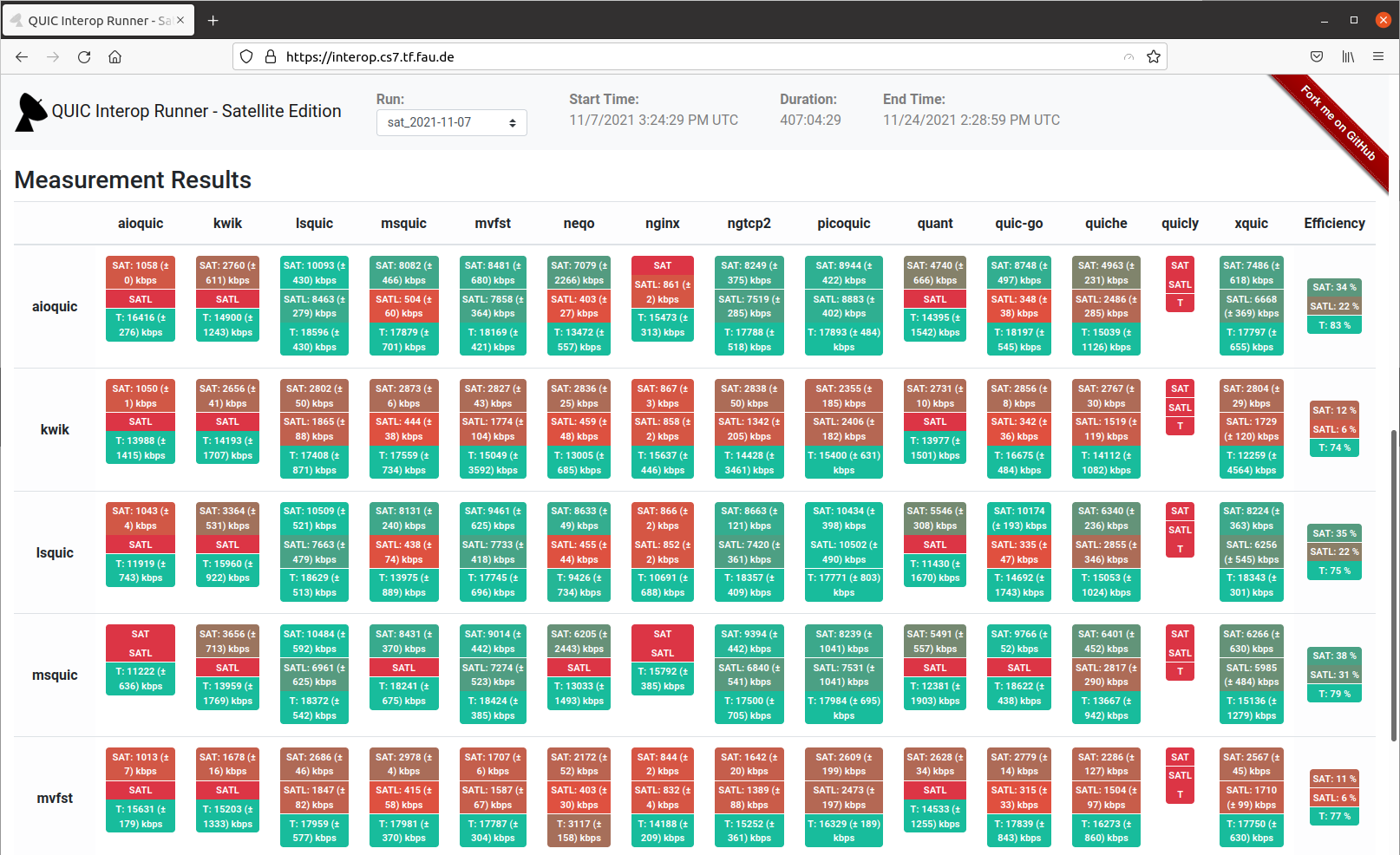
Figure 1: Partial Screenshot of the QIR-SE Website Showing the Measurement Results

Thanks to their wide-area coverage, satellites are the only option for Internet access for some people. Today’s modern geostationary high throughput satellites (GEO) provide data rates up to $100\text{\,}\mathrm{Mbit}\text{/}\mathrm{s}$ in the downlink and even more in the future [1]. However, compared to other Internet access technologies, geostationary satellites suffer from high propagation delays. Together with other delays, Round-Trip Times of $600\text{\,}\mathrm{ms}\text{/}$ and more are typical [2]. Obviously, latency-sensitive applications are inherently problematic for GEO satellites, but also the performance of transport protocols like TCP is problematic over high-delay links because of slow-start and long feedback loops. In order to mitigate poor TCP performance, Performance Enhancing Proxies are deployed in satellite networks [3]. With encrypted transport layer headers, as it is the case for VPNs and QUIC [4], PEP can not be applied anymore. This leads to significant performance degradation described in earlier publications [5, 6, 2, 7, 8, 9, 10] and this work. Research, like [11, 12], that neglects the fact that PEP are usually used to accelerate TCP connections, conclude that QUIC outperforms TCP on these satellite links. This is also confirmed by some of the before mentioned references, which compare QUIC’s performance with TCP used over VPNs. We prepared a more detailed work in progress literature survey which is available online.

The QUIC-Interop-Runner (QIR) [13] is used by the IETF QUIC Working Group for interoperability testing of QUIC implementations. It already supports numerous implementations uniformly packaged into Docker containers and available on Docker Hub. The runner tests every client implementation with every server implementation three times per day and performs several checks, like if a handshake completes successfully, or if 0-RTT works. The following implementations, grouped by their role, were part of the QIR at the time of writing:

• Client & Server: aioquic, kwik, lsquic, msquic, mvfst, neqo, ngtcp2, picoquic, quant, quic-go, quiche, quicly, xquic

• Client only: chrome

• Server only: nginx

For a detailed description of the implementations, please refer to the QIR website or the QUIC Working Group. In the official QIR, chrome was not supported and quicly always failed. These two implementations are thus also ignored in our tests.

The focus of the QIR is on testing interoperability, functionalities, and standards compliance. There are also two performance measurement tests: Goodput uses an emulated low-latency channel with a data rate of $10\text{\,}\mathrm{Mbit}\text{/}\mathrm{s}$ to measure the average goodput for the transfer of a large file, and CrossTraffic measures the goodput with a competing iperf transmission. These non-challenging link parameters lead to good results for almost all implementations, i.e., the achieved goodput is close to the physical layer link rate of $10\text{\,}\mathrm{Mbit}\text{/}\mathrm{s}$. However, real Internet access links, especially geostationary satellite links with high delays, are much more challenging [14]. This motivated us to adapt the QIR to include geostationary satellite links, which we then call QIR-SE. To the best of our knowledge, this is the first time that the performance of a broad range of QUIC implementations over geostationary satellite links is evaluated.

The architecture of QIR and QIR-SE is described in Section II. To gain further insights into realistic use cases, we also conducted tests over real satellite links. The configuration of the emulated satellite links and the used real satellite accesses are described in Section III. Similar to QIR, all results obtained with the QIR-SE are presented on a website⁸, which is shown in Fig. 1. In Section IV results are elaborated, which in addition to the original QIR also include auto-generated time-offset diagrams. Section V concludes this paper and suggests future research.

II Architecture

The architecture of QIR is shown in Fig. 2a. It employs Docker Compose with virtual networks to deploy the entire test environment on a single host machine. Most test cases require a setup of three containers: The QUIC client implementation, the QUIC server implementation and a container containing the ns-3 Network Simulator in between. Additional containers can be deployed for special test cases. For the link emulator, different ns-3 scenarios are used, which are available online. The runner passes TLS keys and certificates [15] through the Docker volume /certs into the end point containers. The implementations have to generate log files in the Docker volume /logs. Servers have to serve files with random content from the volume /www and clients have to download them to the volume /downloads, preferably by using HTTP/0.9, which is very simple and has a minimal overhead. During the run, ns-3 is used to capture packets on the wire into Pcap files. The traces are then analyzed using pyshark, a Python wrapper for tshark from the Wireshark protocol analyzer tool set. As each client implementation is tested with each server implementation, a two-dimensional matrix is filled with test results, which is visualized in Figs. 1 and 4. It is stored as JSON file. We use this information and the captured traces to automatically generate time-offset plots for each combination of implementation afterwards, as shown in Section IV-D.

(a) Architecture of the Original QIR used for Emulations

(b) Distributed Architecture of QIR used for Real Satellite Links

Figure 2: Architecture of The QIR & QIR-SE

II-A Emulation

To emulate satellite links, which have usually different properties in the forward and return path, we added a new asymmetric ns-3 scenario. The data rate, emulated queue size and Packet Loss Rate (PLR) can be configured individually per direction. The artificial delay applies to both directions.

II-B Real Satellite Links

Additionally, we modified the runner to use real network links between the implementations under test. We replaced the deployment mechanism, which was built upon Docker Compose, with direct calls to the Docker API to possibly distributed Docker deamons, as visualized in Fig. 2b. In our setup, we have one dedicated machine per satellite access. QIR-SE picks the according machine per test case to deploy the client. The server is executed on the same machine as the QIR-SE itself. As ns-3 can no longer be used to capture the Pcap traces, we run a tcpdump container per end point, which joins the network of the implementation container on the correspondent host.

III Test Setup

All measurements have been performed on the following systems:

The emulated scenarios have been executed on an Ubuntu 20.04.3 LTS server with Kernel 5.4.0 and Docker 20.10.10. The server is powered by an Intel® Xeon® X5650 CPU and has $16\text{\,}\mathrm{GiB}\text{/}$ of RAM installed.

For measurements with real satellite connections, the server implementations have been executed on the aforementioned machine. The clients have been run on other computers, which are connected to the modems of the satellite link. These computers run Ubuntu 18.04.6 LTS with Kernel 5.4.0 and Docker 20.10.7. Both computers are powered by an Intel® Core™ i5 4590 CPU and $8\text{\,}\mathrm{GiB}\text{/}$ RAM each.

III-A Emulation

We use the Terrestrial scenario, which equals the Goodput scenario in the original QIR, but with an increased data rate of $20\text{\,}\mathrm{Mbit}\text{/}\mathrm{s}$, to compare the satellite scenarios with a terrestrial link. The RTT is $30\text{\,}\mathrm{ms}\text{/}$ and the queue size is 25 packets. Additionally, we added two performance measurement tests with path properties similar to satellite links: Sat and SatLoss. They differ in the artificial PLR, which is set to $0\text{\,}\mathrm{\char 37\relax}\text{/}$ in the first scenario and to $1\text{\,}\mathrm{\char 37\relax}\text{/}$ in the latter one. In both cases, we set the data rate to 20/$2\text{\,}\mathrm{Mbit}\text{/}\mathrm{s}$ (forward / return link) and the one-way delay to $300\text{\,}\mathrm{ms}\text{/}$, which results in an RTT of $600\text{\,}\mathrm{ms}\text{/}$. All emulated test cases have been repeated ten times per combination of implementation.

III-B Real Satellite Links

We also ran measurements using two real end-user satellite accesses: Astra and Eutelsat, which are available in Europe. The satellite dishes and terminals are located at the University of Erlangen-Nürnberg, Martensstr. 3, Erlangen, Germany. Details about the tariffs are listed in Table I. The first one advertises a data rate less than half of the data rate of the second one. While Eutelsat prioritizes traffic up to $60\text{\,}\mathrm{GB}\text{/}$, we did not run into that limit during the measurements. Both operators provide IPv4 connectivity through carrier-grade NAT, and IPv6 is not available. Further testimonials of the products can be found in a previous measurement campaign, where measurements assessed a stable performance of the real satellite links, and the throughput achieves the advertised link rates. To be on the safe side, our measurements were carried out during constantly good weather conditions and paused between potentially congested times (i.e., between 6 p.m. and 11 p.m. local time). Within one run, the execution of client and server combinations was shuffled, and each combination was repeated five times.

TABLE I: Measurements with Real Satellite Access

Test Case	Provider & Tariff	Advertised Data Rate	Traffic Limit	Modem
Astra	Novostream Astra Connect L+	20/$2\text{\,}\mathrm{Mbit}\text{/}\mathrm{s}$	—	Gilat SkyEdge II-c
Eutelsat	Konnect Zen	50/$5\text{\,}\mathrm{Mbit}\text{/}\mathrm{s}$	priorit. up to $60\text{\,}\mathrm{GB}\text{/}$	Hughes HT2000W

IV Evaluation

Before we start with the evaluation, we would like to emphasize that not all implementations might strive for high performance. Some might be only proof of concept implementations, others might have simplicity or resource efficiency as primary goal, and others might not have been optimized for high latency links yet. Yet, the performance degradation compared to the emulated Terrestrial scenario will be clearly visible.

The evaluation is split into four parts. First, we present heatmaps inspired by the QIR-SE website and give an overview considering all results, followed by a discussion whether client or server implementation influences the outcomes more. Next, we try to analyze the impact of different Congestion Control Algorithms. Lastly, we pick specific combinations and present their behavior by means of time-offset graphs.

IV-A Overview

To visualize the result matrices of the measurements generated with the QIR-SE in more detail, we rendered a heatmap for each scenario (Fig. 4). The columns belong to the server implementation and the rows to the clients. We omitted non-functioning implementations. The color scale is normalized to the minimum and maximum observed goodput value of each scenario. The size of the circles are synchronized between all charts. Currently, we only distinguish between unspecified errors (marked with ) and timeouts (marked with $T$).

TABLE II: Overview of Measurement Results
For the columns Mean and Maximum, the absolute goodput values are in the left column and the relative efficiency values in the right column.

Measurement	Mean		Maximum		Timeout $T$	Failed
	$[$\mathrm{Mbit}\text{/}\mathrm{s}$]$	$[$\mathrm{\char 37\relax}\text{/}$]$	$[$\mathrm{Mbit}\text{/}\mathrm{s}$]$	$[$\mathrm{\char 37\relax}\text{/}$]$	$[$\mathrm{\char 37\relax}\text{/}$]$	$[$\mathrm{\char 37\relax}\text{/}$]$
Terrestrial	15.11	76	19.2	96	12	1
Sat	5.05	25	12.0	60	3	6
SatLoss	3.06	15	11.5	57	13	17
Astra	4.91	25	13.5	68	23	15
Eutelsat	6.98	14	17.5	35	20	11

Figure 3: CDFs Using Normalized Efficiency Values as Defined in Equation 1

(a) Average Goodput of Measurement Sat

(b) Average Goodput of Measurement SatLoss

(c) Average Goodput of Measurement Astra

(d) Average Goodput of Measurement Eutelsat

Figure 4: Result Matrices (: Unspecified Error, $T$: Timeout)

In addition to the heatmaps, we gathered the measurement results in Table II and as Cumulative Distribution Functions in Fig. 3. For each scenario, the table shows the mean and maximum value of all experiments and the amount of combinations that either ran into a timeout or failed for an unknown reason. On the left side of each column, the absolute goodput values are used (as in the heatmaps). On the right side, as well as in the CDF, we use the efficiency, which is defined as the goodput value divided by the emulated or advertised link data rate:

$$\text{Efficiency}=\frac{\text{Goodput}}{\text{Link Data Rate}}$$ (1)

Besides the emulated satellite scenarios Sat and SatLoss and the real satellite links Astra and Eutelsat, the table and the CDF plot also contain the results for the Terrestrial scenario as reference. Unsuccessful runs are not considered in the calculation of the mean values in Table II but plotted as $0\text{\,}\mathrm{\char 37\relax}\text{/}$ efficiency in the CDF in Fig. 3.

First, we take a look at the high number of failed experiments for all scenarios. The number of failures and timeouts is rather high in the Terrestrial scenario because of neqo, which did not work as a client in this scenario for unknown reasons, although it worked in our satellite scenarios. The reason lsquic fails as a server when measuring with real satellite links is technical and caused by the Docker image provided by the maintainers. In the SatLoss, Astra and Eutelsat scenarios we can see a lot of implementations, that were not able to transfer the test file of $10\text{\,}\mathrm{MiB}\text{/}$ via the corresponding links. A more detailed analysis of the reasons of failures is subject to future work.

As one can see in Table II and Fig. 3, the Terrestrial scenario achieves goodput values close to the link rate. This is not the case for geostationary satellite scenarios. Instead, there are significant differences between implementations.

Although Sat, shown in Fig. 4a, has stable link emulation and no artificial loss, there is a lot of variance in the achieved goodput. Some implementations perform significantly better than the others. Yet, the achieved goodput is far below the advertised link rate of $20\text{\,}\mathrm{Mbit}\text{/}\mathrm{s}$. In half of the measurements, it is even below $25\text{\,}\mathrm{\char 37\relax}\text{/}$ of the link data rate. When all entries of a row (respectively column) show poor results, the implementation performs poor as client (respectively server). A more detailed analysis of the client vs. server performance of the Sat scenario is given in Section IV-B.

SatLoss performs worst among all scenarios when considering the absolute goodput values, see Table II. Figure 4b shows which implementations suffer most from the $1\text{\,}\mathrm{\char 37\relax}\text{/}$ artificial PLR added to the emulated satellite link. Compared to the no-loss scenario, many implementations do either not finish a transmission successfully or achieve considerably lower goodput rates. The efficiency decreases from only $25\text{\,}\mathrm{\char 37\relax}\text{/}$ in the Sat scenario to even less in the SatLoss scenario ($15\text{\,}\mathrm{\char 37\relax}\text{/}$). There are only a few combinations that perform well in the SatLoss scenario, with picoquic as client and server for example being more thoroughly analyzed later in Section IV-D1.

The performance of the real satellite operators is visualized in more breadth in Fig. 4c (Astra) and Fig. 4d (Eutelsat). The PLR on these real satellite links is usually very low¹⁶, but higher dynamics can be expected on real links. Compared to the Sat scenario, this results in less combinations finishing successfully and lower goodput values. There is a correlation between the results for Astra and Eutelsat, i.e., most combinations perform similarly on both systems. Eutelsat reaches the highest mean and maximum goodput rates in our tests (note different scale in Fig. 4d). However, given the forward link data rates (Eutelsat $50\text{\,}\mathrm{Mbit}\text{/}\mathrm{s}$ vs. other satellite scenarios with $20\text{\,}\mathrm{Mbit}\text{/}\mathrm{s}$), the efficiency of Eutelsat is with about $14\text{\,}\mathrm{\char 37\relax}\text{/}$ on average actually worse than Astra ($25\text{\,}\mathrm{\char 37\relax}\text{/}$). This shows that more bandwidth does not automatically result in a better performance by the same factor. The link utilization on both real satellite links is very low, similar to the results of our simulated test cases.

IV-B Client vs. Server Implementation

Figure 5: Violin Plots for Each Implementation in the Sat Scenario. Horizontal Lines represent the Quartiles $Q_{1}$, $Q_{2}$ and $Q_{3}$.

As the server has to send most of the data and therefore has to estimate the channel parameters and especially the bottleneck bandwidth, it seems likely that the performance of the transmission is mainly determined by the server. However, the result matrices in Fig. 4 show no pattern that confirms this assumption, instead both the client and the server contribute to the overall performance of a QUIC connection.

In order to verify this statement, we draw violin plots as shown in Fig. 5. Due to space limitations, we only present the plot for the Sat scenario. Other scenarios lead to similar results. The orange graphs show the performance of a specific server implementation tested with all clients, and the blue graph shows the performance of a specific client implementation tested with all servers.

Again, it can be seen that the achieved goodput is far off the emulated link rate. It also becomes clearer, that kwik does neither perform well as client nor as server, aioquic performs well if used as client but not as server, and mvfst and ngtcp2 perform well if used as server but not as client. An interesting observation from Fig. 5 is that results are often concentrated towards one end of the distribution. Especially when looking at the server role, this means that these server implementations either result in very good or very poor results. Thus, we conclude that both the client and the server contribute to the overall performance of a QUIC connection.

IV-C Impact of the Congestion Control Algorithm

TABLE III: Implementations and their CCAs.
Algorithms are determined by hand and must be taken with caution. The default CCA is printed bold.

Name	CCA	HyStart
aioquic	NewReno
chrome	BBRv2, CUBIC
kwik	NewReno
lsquic	BBR, CUBIC
msquic	CUBIC
mvfst	BBR, CUBIC, NewReno, …
neqo	CUBIC, NewReno
nginx	?⃝
ngtcp2	BBRv2, BBR, CUBIC, Reno
picoquic	BBR, CUBIC
quant	NewReno
quic-go	CUBIC ?⃝, Reno ?⃝
quiche	CUBIC
quicly	CUBIC, Reno, pico
xquic	BBR, CUBIC, Reno

Figure 6: Relation of Measurement Results Between Sat & SatLoss
Points are colored according to the CCA of the server implementation.

As we assume that the CCA of the server implementation has a large impact on the performance of a connection, we determined the supported algorithms and collected them in Table III. For each implementation, we tried to identify all implemented algorithms and the default one by inspecting the available command line flags of the implementations in the Docker images used by the runner or the corresponding code if available. As there is no database or standardized interface to query the CCAs, it is not guaranteed that the information in Table III is correct. Additionally, it should be noted that the coding and parametrization of the same CCAs might differ substantially among implementations.

Figure 6 displays a relational plot of the measurement results from the Sat scenario (horizontal) and the SatLoss scenario (vertical). Again, we use the normalized efficiency values as defined in Eq. 1. Each point corresponds to the mean of the efficiencies achieved by the corresponding implementation tuple over all ten iterations in the corresponding scenario. Two clusters of measurement results can be identified: The first ([regular] brown) one shows no correlation between both experiments. While there are medium results in the Sat scenario, the results achieved in the SatLoss scenario (with a PLR of $1\text{\,}\mathrm{\char 37\relax}\text{/}$) are altogether very poor. The other group ([regular] turquoise) shows a correlation between both experiments, and the results in SatLoss are quite similar and only slightly poorer than in Sat.

We use the previously determined CCAs to color the points in that plot according to the algorithm used by the server implementation. In the turquoise group of data points achieving a link utilization of more than $10\text{\,}\mathrm{\char 37\relax}\text{/}$ in the SatLoss scenario, there are only combinations where the server uses CUBIC or BBR. The other group contains combinations with Reno, NewReno and CUBIC.

This could be an indication for CUBIC and BBR working better in lossy scenarios than Reno and NewReno. However, it might also be possible that implementations that employ one of the much more complex CCAs are more optimized in general. It is hard to draw a more precise conclusion without deeper knowledge of the code of the implementations.

IV-D Time-Offset Graphs

While we try to render and annotate time-offset plots using captured Pcap traces, this does not succeed for every combination for various reasons. For example, some combinations do not use UDP port 443, some use HTTP/3 instead of HTTP/0.9 as requested by the runner, or there are issues with standard compliance. In this section, we chose five plots that show interesting behavior and discuss them in more detail. More plots can be found on our website⁸. In every plot there are the traces of all iterations of the same implementation tuple in the according measurement scenario (ten for Sat and SatLoss, five for Astra and Eutelsat). That one with the medium time to completion is highlighted colored. The others are gray. If an offset number is transmitted the first time, the corresponding point in the plot is colored blue. Retransmissions are colored orange.

IV-D1 picoquic—picoquic—SatLoss

Compared to the other implementations, picoquic often achieves good results. It seems to be built with satellite use-cases in mind. Even in challenging scenarios, the transmission makes steady progress. Figure 7 shows the transmission of picoquic as client and as server in the SatLoss scenario—the simulated scenario with $1\text{\,}\mathrm{\char 37\relax}\text{/}$ PLR. According to our analysis in Table III, BBR was used in this transmission. As soon as the bottleneck bandwidth is estimated, the data is transmitted sequentially at a fairly constant rate and single lost packets are re-transmitted out-of-order. Picoquic seems to automatically retransmit the last bytes of the file multiple times to avoid waiting one RTT until the client can signal a loss. The entire transmission takes slightly more than $7\text{\,}\mathrm{s}\text{/}$. This equals a goodput of slightly more than $11\text{\,}\mathrm{Mbit}\text{/}\mathrm{s}$ which equals a link utilization of slightly more than $50\text{\,}\mathrm{\char 37\relax}\text{/}$.

Figure 7: Time-Offset Plot of Picoquic—Picoquic—SatLoss

IV-D2 kwik—msquic—Sat

The example in Fig. 8, with kwik as server using NewReno as CCA, shows a slow startup phase of about $11\text{\,}\mathrm{s}\text{/}$. Most implementations that are not optimized for satellite scenarios have this in common. Some implementations, like aioquic, even never reach a steady state. In this example there is a second striking behavior: In some iterations, the final transmission rate is set to a much smaller value than in other iterations. This results in very different time to completions between iterations of the same experiment—even though no nondeterministic packet losses are emulated in the Sat test case. Additionally, the jagged curves indicate bad pacing.

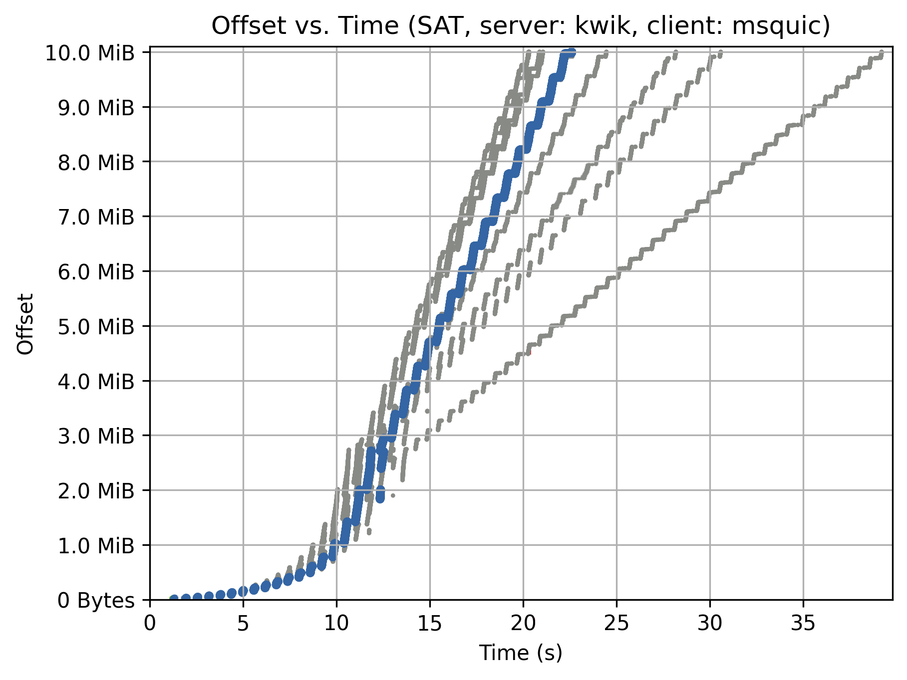
Figure 8: Time-Offset Plot of Kwik—Msquic—Sat

IV-D3 lsquic—xquic—Sat

The analysis of the transmissions shown in Fig. 9 reveals remarkably many retransmissions. Since no artificial losses are introduced in the Sat scenario, the retransmissions might indicate a bug in either of the implementations. However, some sequence numbers in the range between 3 and $4\text{\,}\mathrm{MiB}\text{/}$ seem not to be used sequentially. The second almost vertical line in this range is not drawn in orange, which indicates that the according packets are no retransmitted ones. Such behavior should be analyzed in the future.

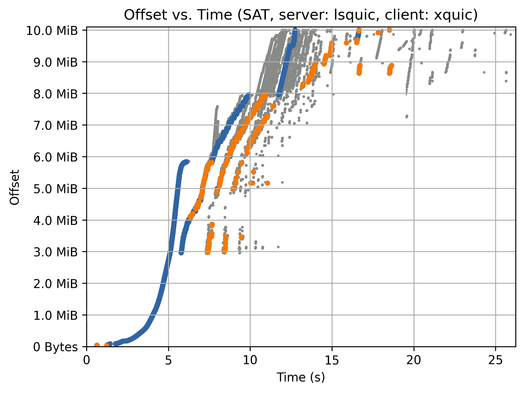
Figure 9: Time-Offset Plot of Lsquic—Xquic—Sat

IV-D4 msquic—xquic—SatLoss

The plot in Fig. 10 shows very different but high values for the time to completion in the SatLoss scenario. According to Table III, loss-based CUBIC was (most likely) used in this scenario. The losses lead to high drops of the data rate and recovery seems to be very slow probably due to the high RTT. When many losses occur in quick succession, the data rate is throttled more heavily. When losses indicate congestion, it is fine to throttle the transmission rate. However, when packets get lost due to temporary effects on a path segment, there is no benefit in reducing the transmission data rate. Instead, doing so has a severe impact on the performance via the satellite link.

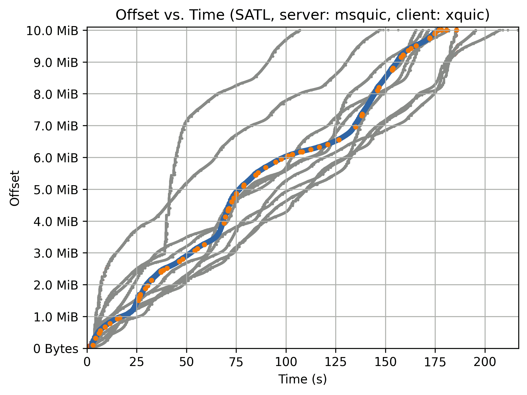
Figure 10: Time-Offset Plot of Msquic—Xquic—SatLoss

IV-D5 picoquic—ngtcp2—Astra

A way to avoid dreaded retransmissions is sending each packet multiple times even when it was not lost. This can speed up the transmission because it is not necessary to wait for the ACK of the recipient, which has proven to be beneficial in previous Section IV-D1 where picoquic was used as server, too. On the other hand, this optimization causes additional traffic on the link and thus should be used carefully. In Fig. 11, it can be observed that such optimistic retransmissions leads to lots of redundantly sent data, because every packet is retransmitted six to eight times. Although only a file of $10\text{\,}\mathrm{MiB}\text{/}$ is transferred, this leads to approximately $6080\text{\,}\mathrm{MiB}\text{/}$ of data being sent.

Figure 11: Time-Offset Plot of Picoquic—Ngtcp2—Astra

V Conclusion and Future Work

Due to the non-applicability of PEP, the performance of QUIC via geostationary satellite links depends mainly on the end points. We presented a tool based on the QIR that allows running measurements via real and emulated satellite links with numerous QUIC implementations. It also automatically generates time-offset plots for more detailed analysis. Our results show that differences between implementations are very high. Many implementations even fail to transfer a medium-sized file over satellite links. The successful ones usually achieve a very poor goodput. The performance is even poorer when artificial packet losses are introduced. Increasing the link data rate does not automatically increase the achieved goodput in the same ratio. According to the results of the combinations of implementations, we can conclude that both the server and the client contribute to the overall performance of the transmission.

Regarding future work, multiple directions can be thought of. Additional performance test cases (e.g., short transfers of small objects, enabling explicit congestion notification, fairness tests, etc.) would provide more insights into the performance of QUIC over satellite networks. This should also include different parameters for QUIC protocol stacks [14] and extensions like the 0-RTT-BDP draft [16]. Testing could include more satellite systems, including both geostationary and Low Earth Orbit (LEO) megaconstellation satellite systems (e.g., Starlink). Finally, long-term measurements would be helpful to track changes of QUIC implementations. This should also include investigations regarding the high number of unsuccessful runs observed in the QIR-SE.

All Internet links were last accessed on 2022-02-12.

References

- [1] R. De Gaudenzi, P. Angeletti, D. Petrolati, and E. Re, “Future technologies for very high throughput satellite systems,” International Journal of Satellite Communications and Networking, vol. 38, no. 2, pp. 141–161, 2020. [Online]. Available: https://onlinelibrary.wiley.com/doi/abs/10.1002/sat.1327
- [2] J. Deutschmann, K.-S. Hielscher, and R. German, “Satellite Internet Performance Measurements,” in 2019 International Conference on Networked Systems (NetSys), Mar. 2019, pp. 1–4. [Online]. Available: https://ieeexplore.ieee.org/abstract/document/8854494
- [3] J. Griner, J. Border, M. Kojo, Z. D. Shelby, and G. Montenegro, “Performance Enhancing Proxies Intended to Mitigate Link-Related Degradations,” Internet Engineering Task Force, Request for Comments RFC 3135, Jun. 2001. [Online]. Available: https://datatracker.ietf.org/doc/rfc3135
- [4] J. Iyengar and M. Thomson, “QUIC: A UDP-Based Multiplexed and Secure Transport,” Internet Engineering Task Force, Request for Comments RFC 9000, May 2021. [Online]. Available: https://datatracker.ietf.org/doc/rfc9000
- [5] R. Secchi, A. Mohideen, and G. Fairhurst, “Evaluating the Performance of Next Generation Web Access via Satellite,” in Wireless and Satellite Systems, P. Pillai, Y. F. Hu, I. Otung, and G. Giambene, Eds. Cham: Springer International Publishing, 2015, pp. 163–176. [Online]. Available: https://link.springer.com/chapter/10.1007/978-3-319-25479-1_12
- [6] L. Thomas, E. Dubois, N. Kuhn, and E. Lochin, “Google QUIC performance over a public SATCOM access,” International Journal of Satellite Communications and Networking, vol. 37, no. 6, pp. 601–611, 2019. [Online]. Available: https://onlinelibrary.wiley.com/doi/abs/10.1002/sat.1301
- [7] C. Mogildea, J. Deutschmann, K.-S. Hielscher, and R. German, “QUIC over Satellite: Introduction and Performance Measurements,” in KaConf, Sep. 2019, p. 9. [Online]. Available: https://www.researchgate.net/publication/351282748_QUIC_OVER_SATELLITE_INTRODUCTION_AND_PERFORMANCE_MEASUREMENTS
- [8] J. Border, B. Shah, C.-J. Su, and R. Torres, “Evaluating QUIC’s Performance Against Performance Enhancing Proxy over Satellite Link,” in 2020 IFIP Networking Conference (Networking), Jun. 2020, pp. 755–760. [Online]. Available: https://ieeexplore.ieee.org/abstract/document/9142718/
- [9] N. Kuhn, F. Michel, L. Thomas, E. Dubois, and E. Lochin, “QUIC: Opportunities and threats in SATCOM,” in 2020 10th Advanced Satellite Multimedia Systems Conference and the 16th Signal Processing for Space Communications Workshop (ASMS/SPSC), Oct. 2020, pp. 1–7. [Online]. Available: https://ieeexplore.ieee.org/abstract/document/9268814
- [10] A. Custura, T. Jones, and G. Fairhurst, “Impact of Acknowledgements using IETF QUIC on Satellite Performance,” in 2020 10th Advanced Satellite Multimedia Systems Conference and the 16th Signal Processing for Space Communications Workshop (ASMS/SPSC), Oct. 2020, pp. 1–8. [Online]. Available: https://ieeexplore.ieee.org/document/9268894
- [11] S. Yang, H. Li, and Q. Wu, “Performance Analysis of QUIC Protocol in Integrated Satellites and Terrestrial Networks,” in 2018 14th International Wireless Communications Mobile Computing Conference (IWCMC), Jun. 2018, pp. 1425–1430. [Online]. Available: https://ieeexplore.ieee.org/document/8450388
- [12] H. Zhang, T. Wang, Y. Tu, K. Zhao, and W. Li, “How Quick Is QUIC in Satellite Networks,” in Communications, Signal Processing, and Systems, ser. Communications, Signal Processing, and Systems, Q. Liang, J. Mu, M. Jia, W. Wang, X. Feng, and B. Zhang, Eds. Singapore: Springer Singapore, Jun. 2018, pp. 387–394. [Online]. Available: https://link.springer.com/chapter/10.1007/978-981-10-6571-2_47
- [13] M. Seemann and J. Iyengar, “Automating QUIC Interoperability Testing,” in Proceedings of the Workshop on the Evolution, Performance, and Interoperability of QUIC, ser. EPIQ ’20. New York, NY, USA: Association for Computing Machinery, Aug. 2020, pp. 8–13. [Online]. Available: https://doi.org/10.1145/3405796.3405826
- [14] T. Jones, G. Fairhurst, N. Kuhn, J. Border, and S. Emile, “Enhancing Transport Protocols over Satellite Networks,” Internet Engineering Task Force, Internet Draft draft-jones-tsvwg-transport-for-satellite-02, Oct. 2021, work in Progress. [Online]. Available: https://datatracker.ietf.org/doc/draft-jones-tsvwg-transport-for-satellite/02/
- [15] E. Rescorla, “The Transport Layer Security (TLS) Protocol Version 1.3,” Internet Engineering Task Force, Request for Comments RFC 8446, Aug. 2018. [Online]. Available: https://datatracker.ietf.org/doc/rfc8446
- [16] N. Kuhn, S. Emile, G. Fairhurst, T. Jones, and C. Huitema, “Transport parameters for 0-RTT connections,” Internet Engineering Task Force, Internet Draft draft-kuhn-quic-0rtt-bdp-11, Oct. 2021, work in Progress. [Online]. Available: https://datatracker.ietf.org/doc/draft-kuhn-quic-0rtt-bdp/11/