Catalyzation of supersolidity in binary dipolar condensates

Abstract

Breakthrough experiments have newly explored the fascinating physics of dipolar quantum droplets and supersolids. The recent realization of dipolar mixtures opens further intriguing possibilities. We show that under rather general conditions, the presence of a second component catalyzes droplet nucleation and supersolidity in an otherwise unmodulated condensate. Droplet catalyzation in miscible mixtures, which may occur even for a surprisingly small impurity doping, results from a local roton instability triggered by the doping-dependent modification of the effective dipolar strength. The catalyzation mechanism may trigger the formation of a two-fluid supersolid, characterized by a generally different superfluid fraction of each component, which opens intriguing possibilities for the future study of spin physics in dipolar supersolids.

Supersolids constitute an intriguing state of matter that combines superfluidity and the crystalline order characteristic of a solid Boninsegni2012 . Whereas this long-sought phase has remained elusive in Helium Chan2013 , recent developments on ultra-cold gases have opened new possibilities for its realization. Bose-Einstein condensates with spin-orbit coupling Li2017 ; Putra2020 ; Geier2021 and in optical cavities Leonard2017 have revealed supersolid features. Recently, breakthrough experiments on condensates formed by highly magnetic atoms have created dipolar supersolids with an interaction-induced crystalline structure Review2021 ; Review2022 .

Dipolar supersolids are closely linked to the idea of quantum droplets, a novel ultra-dilute quantum liquid that results from the combination of competing, and to large extend cancelling, mean-field interactions, and the stabilization provided by quantum fluctuations (quantum stabilization) Petrov2015 . In dipolar condensates Review2021 ; Review2022 , the competition between strong dipolar interactions and contact-like interactions provides the crucial mean-field quasi-cancellation. Quantum stabilization arrests mean-field collapse leading to self-bound droplets Kadau2016 ; Chomaz2016 ; Schmitt2016 . Due to the anisotropy and non-locality of the dipolar interaction, confinement leads to the formation of a droplet array Wenzel2017 , which for properly fine-tuned contact interactions remains superfluid, hence realizing a supersolid Tanzi2019 ; Boettcher2019 ; Chomaz2019 ; Natale2019 ; Tanzi2019b ; Guo2019 . The recent creation of two-dimensional dipolar supersolids Norcia2021 ; Bland2021 opens further fascinating perspectives, as exotic pattern formation Zhang2019 ; Zhang2021 ; Hertkorn2021 ; Poli2021 and quantum vortices Gallemi2020 ; Roccuzzo2020 .

Quantum droplets have been also realized in non-dipolar binary mixtures due to competing mean-field intra- and inter-component contact interactions and quantum stabilization Cabrera2018 ; Semeghini2018 ; DErrico2019 . Crucially, droplet formation requires miscible components with a fixed ratio between their densities given by the ratio of intra-component scattering lengths Petrov2015 . Hence, the mixture behaves as a single-component condensate. Moreover, the short-range isotropic character of the interactions prevents the formation of droplet arrays and supersolids, although self-bound supersolid stripes may be realized in the presence of spin-orbit coupling Sachdeva2020 ; Sanchez-Baena2020 .

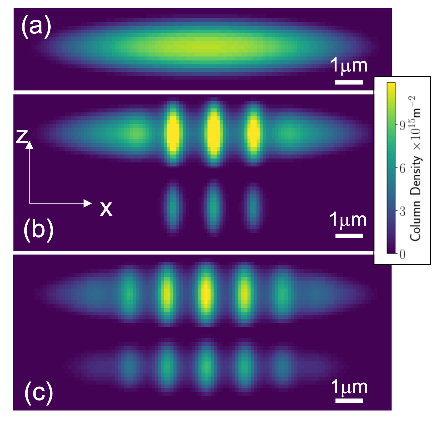
Figure 1: Binary mixture with $N=63000$ ¹⁶⁴Dy atoms, $\omega_{x,y,z}=2\pi(33,110,167)\,\mathrm{Hz}$, $\mu_{1}=10\mu_{B}$, $\mu_{2}=9\mu_{B}$, and $a_{11}=a_{22}=100a_{0}$. (a) Column density (integrated along $y$) for $N_{2}=0$. (b) Column density of component 1 (top) and 2 (bottom) for $a_{12}=62.5a_{0}$ and $N_{2}/N=0.1$ (SS-ID regime). (c) Same for $a_{12}=67.5a_{0}$ and $N_{2}/N=0.3$ (SS-SS regime). In Figs. (b) and (c) the components are shifted along $z$ for visualization purposes.

Recent experiments have realized for the first time mixtures of two dipolar species Trautmann2018 ; Durastante2020 ; Politi2021 , opening exciting new possibilities. In contrast to non-dipolar mixtures, dipolar droplets may occur for an arbitrary relative population of the components, which may be both miscible and immiscible Bisset2021 ; Smith2021 ; Smith2021b . Interestingly, the presence of a second dipolar component may lead to the formation of droplets. Recent numerical results have shown that the increase of inter-species contact interactions in an Er-Dy mixture in the presence of gravitational sag may lead to droplet nucleation in one of the components Politi2021 ; footnote-Modugno .

In this Letter, we discuss, how doping an unmodulated condensate with a second miscible component induces a local modification of the relative dipolar strength, which may result, even for a tiny doping, in a local roton instability that triggers droplet nucleation and supersolidity in both components. The resulting two-fluid supersolid, characterized by a generally different superfluid character of each component, constitutes a rich novel scenario that opens intriguing possibilities for the future study of the interplay between the density and the spin degrees of freedom in dipolar supersolids.

Model.–

We consider two bosonic components, $\sigma=\{1,2\}$, formed by magnetic atoms (a similar formalism applies to electric dipoles). The components may be either two different atomic species, as e.g. erbium and dysprosium Trautmann2018 ; Durastante2020 ; Politi2021 , or atoms of the same species in different internal states, e.g. ¹⁶⁴Dy in different spin states, which is the case we employ below to illustrate the possible physics. Using the formalism of Ref. Bisset2021 , we evaluate the Lee-Huang-Yang (LHY) energy density in an homogeneous binary mixture with densities $n_{1,2}$ (assuming equal masses $m_{1,2}=m$):

$$\xi_{\mathrm{LHY}}(n_{1,2})\!=\!\!\frac{16}{15\sqrt{2\pi}}\!\left(\frac{m}{4\pi\hbar^{2}}\right)^{\!\!\frac{3}{2}}\!{\cal R}\!\left[\!\int_{0}^{1}\!\!\!du\!\sum_{\lambda=\pm}V_{\lambda}(u,n_{1},n_{2})^{\!\frac{5}{2}}\!\right],$$ (1)

with ${\cal R}[\,]$ the real part, and

$$V_{\pm}(u,n_{1},n_{2})\!=\!\!\sum_{\sigma=1,2}\!\!\eta_{\sigma\sigma}n_{\sigma}\pm\sqrt{(\eta_{11}n_{1}\!-\!\eta_{22}n_{2})^{2}\!+\!4\eta_{12}^{2}n_{1}n_{2}},$$ (2)

where $\eta_{\sigma\sigma^{\prime}}(u)=g_{\sigma\sigma^{\prime}}+g_{\sigma\sigma^{\prime}}^{d}(3u^{2}-1)$. The contact-like interactions between components $\sigma$ and $\sigma^{\prime}$ are characterized by the coupling constant $g_{\sigma\sigma^{\prime}}\equiv\frac{4\pi\hbar^{2}a_{\sigma\sigma^{\prime}}}{m}$, with $a_{\sigma\sigma^{\prime}}$ the corresponding $s$-wave scattering length. The strength of the dipole-dipole interactions between components $\sigma$ and $\sigma^{\prime}$ is given by $g_{\sigma\sigma^{\prime}}^{d}\equiv\frac{\mu_{0}\mu_{\sigma}\mu_{\sigma^{\prime}}}{3}\equiv\frac{4\pi\hbar^{2}a_{\sigma\sigma^{\prime}}^{d}}{m}$, where $\mu_{\sigma}$ is the magnetic dipole moment of component $\sigma$, and $\mu_{0}$ is the vacuum permeability. Below we fix $\mu_{1}=10\mu_{B}$ and $\mu_{2}=9\mu_{B}$, with $\mu_{B}$ the Bohr magneton. In order to study spatially inhomogeneous dipolar mixtures we apply the local-density approximation to the LHY term, obtaining the energy functional:

$$E = \int d^{3}r\left[\sum_{\sigma}\psi_{\sigma}^{*}(\vec{r})\left(\frac{-\hbar^{2}\nabla^{2}}{2m}+V_{\mathrm{trap}}(\vec{r})\right)\psi_{\sigma}(\vec{r})\right\delimiter 00$$ (3)

$$+ \frac{1}{2}\sum_{\sigma,\sigma^{\prime}}g_{\sigma\sigma^{\prime}}n_{\sigma}(\vec{r})n_{\sigma^{\prime}}(\vec{r})+\xi_{\mathrm{LHY}}[n_{1}(\vec{r}),n_{2}(\vec{r})]$$

$$+ \left\delimiter 00\sum_{\sigma,\sigma^{\prime}}\frac{3g_{\sigma\sigma^{\prime}}^{d}}{8\pi}\int d^{3}r^{\prime}U_{dd}(\vec{r}-\vec{r}^{\prime})n_{\sigma^{\prime}}(\vec{r}\,^{\prime})n_{\sigma}(\vec{r})\right],$$

with $V_{\mathrm{trap}}(\vec{r})=\frac{m}{2}\left(\omega_{x}^{2}x^{2}+\omega_{y}^{2}y^{2}+\omega_{z}^{2}z^{2}\right)$, $n_{\sigma}(\vec{r})=|\psi_{\sigma}(\vec{r})|^{2}$, and $U_{dd}(\vec{r})=\frac{1}{r^{3}}(1-3\cos^{2}\theta)$, with $\theta$ the angle between $\vec{r}$ and the dipole moments. The ground-state of a mixture with $N_{\sigma}$ atoms in component $\sigma$, with a total atom number $N=N_{1}+N_{2}$, is obtained from the coupled extended Gross-Pitaevskii equations (eGPE):

$$\tilde{\mu}_{\sigma}\psi_{\sigma}(\vec{r})=\frac{\partial E}{\partial\psi_{\sigma}^{*}(\vec{r})},$$ (4)

where $\int d^{3}r\,n_{\sigma}(\vec{r})=N_{\sigma}$ and $\tilde{\mu}_{\sigma}$ is the chemical potential of component $\sigma$. We consider below an elongated trap, with $\omega_{x,y,z}=2\pi\times(33,110,167)\,\mathrm{Hz}$, and $N=63000$ atoms. Similar values have been employed in recent experiments Norcia2021 .

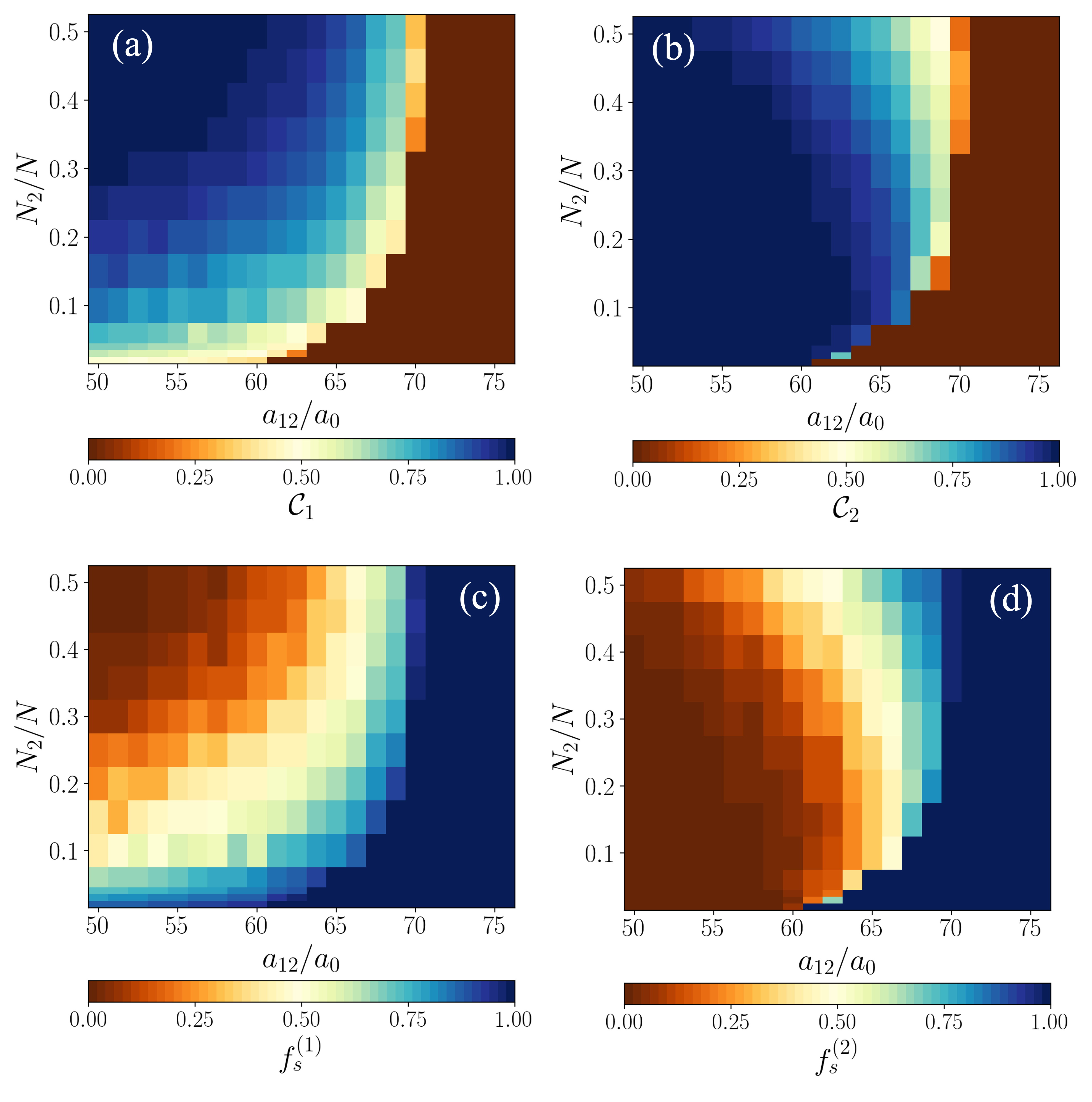
Figure 2: (a,b) Contrast of components 1 and 2, respectively, as a function of $a_{12}/a_{11}$ and $N_{2}/N$. (c,d) Superfluid fraction of components 1 and 2, respectively. The parameters are the same as in Fig. 1.

Doping-induced supersolidity.–

Single-component dipolar condensates in elongated traps present three possible ground-states: the unmodulated (U) regime, without density modulation, at large-enough scattering length $a$; the incoherent-droplet (ID) regime, an incoherent linear droplet at low-enough $a$; and the supersolid (SS) regime, a coherent droplet array in a narrow intermediate window of values of $a$.

In order to illustrate the new possibilities for droplet nucleation and supersolidity in dipolar mixtures, we consider in the following $a_{11}=100a_{0}$ such that, in absence of component 2, component $1$ is well in the U regime (Fig. 1(a)), which demands $a_{11}>94a_{0}$. Although below we provide a more general picture, we fix at this point $a_{22}=a_{11}$ for simplicity. We evaluate the ground-state of the mixture as a function of the doping $N_{2}/N$ and $a_{12}$. We focus on the case in which $a_{12}$ is low-enough, such that the mixture remains miscible.

For a sufficiently large $a_{12}$ ($>72a_{0}$ in the case considered) the binary mixture remains unmodulated (U regime). In contrast, for $a_{12}<72a_{0}$ and a sufficiently large $N_{2}/N$, droplet nucleation leads to a density modulation in both components. The spatial modulation of the density profile of component $\sigma$ is best characterized using the contrast, determined from the maximal and minimal density in the central region ($|x|<L=2\mu\mathrm{m}$ in our calculations), $n_{\sigma,\mathrm{max}}$ and $n_{\sigma,\mathrm{min}}$, as ${\cal C}_{\sigma}=(n_{\sigma,\mathrm{max}}-n_{\sigma,\mathrm{min}})/(n_{\sigma,\mathrm{max}}+n_{\sigma,\mathrm{min}})$. The contrast for components 1 and 2 is depicted in Figs. 2 (a) and (b). The superfluid fraction in each component, $f_{s}^{(\sigma)}$, may be estimated using Legget’s upper bound in the central window Legget1970 ; Legget1998 :

$$f_{s}^{(\sigma)}=(2L)^{2}\left[\int_{-L}^{L}dx\tilde{n}_{\sigma}(x)\int_{-L}^{L}dx\frac{1}{\tilde{n}_{\sigma}(x)}\right]^{-1},$$ (5)

with $\tilde{n}_{\sigma}(x)=\iint\,dy\,dz\,n_{\sigma}(\vec{r})$. For components of equal mass, the overall superfluid fraction, $f_{s}=\frac{N_{1}}{N}f_{s}^{(1)}+\frac{N_{2}}{N}f_{s}^{(2)}$, characterizes the reduction of the overall momentum of inertia, as would be measured via e.g. the response to a component-independent scissors-like perturbation Tanzi2021 ; Norcia2021b ; Roccuzzo2022 ; footnote-CounterMotion .

For sufficiently low $a_{12}$, both components form incoherent droplet arrays (ID-ID regime). The contrasts approach their maximum ${\cal C}_{1,2}\simeq 1$, and $f_{s}^{(1,2)}\simeq 0$. As for other scenarios of dipolar droplets Tanzi2019 ; Boettcher2019 ; Chomaz2019 , the contrasts are significantly lower (and $f_{s}^{(1,2)}$ significantly higher) close to the transition into the U regime, marking the SS-SS regime, in which the droplets of both components remain coherently linked. Note, that ${\cal C}_{1}$ and ${\cal C}_{2}$ follow a different dependence on $N_{2}/N$. Droplets in component 1 (2) may remain coherent, while those in component 2 (1) are in the ID regime, determining the SS-ID (ID-SS) regimes (see Fig. 1(b) and footnote-SM ). Defining the ID regime as having a contrast ${\cal C}>0.96$ footnote-C , we determine the ground-state diagram of Fig. S5 (for a discussion of the overall superfluidity and the relative contribution to each component to it, see footnote-SM ). Interestingly, for low-enough $a_{12}$, a surprisingly small $N_{2}/N$ is enough to induce droplet nucleation.

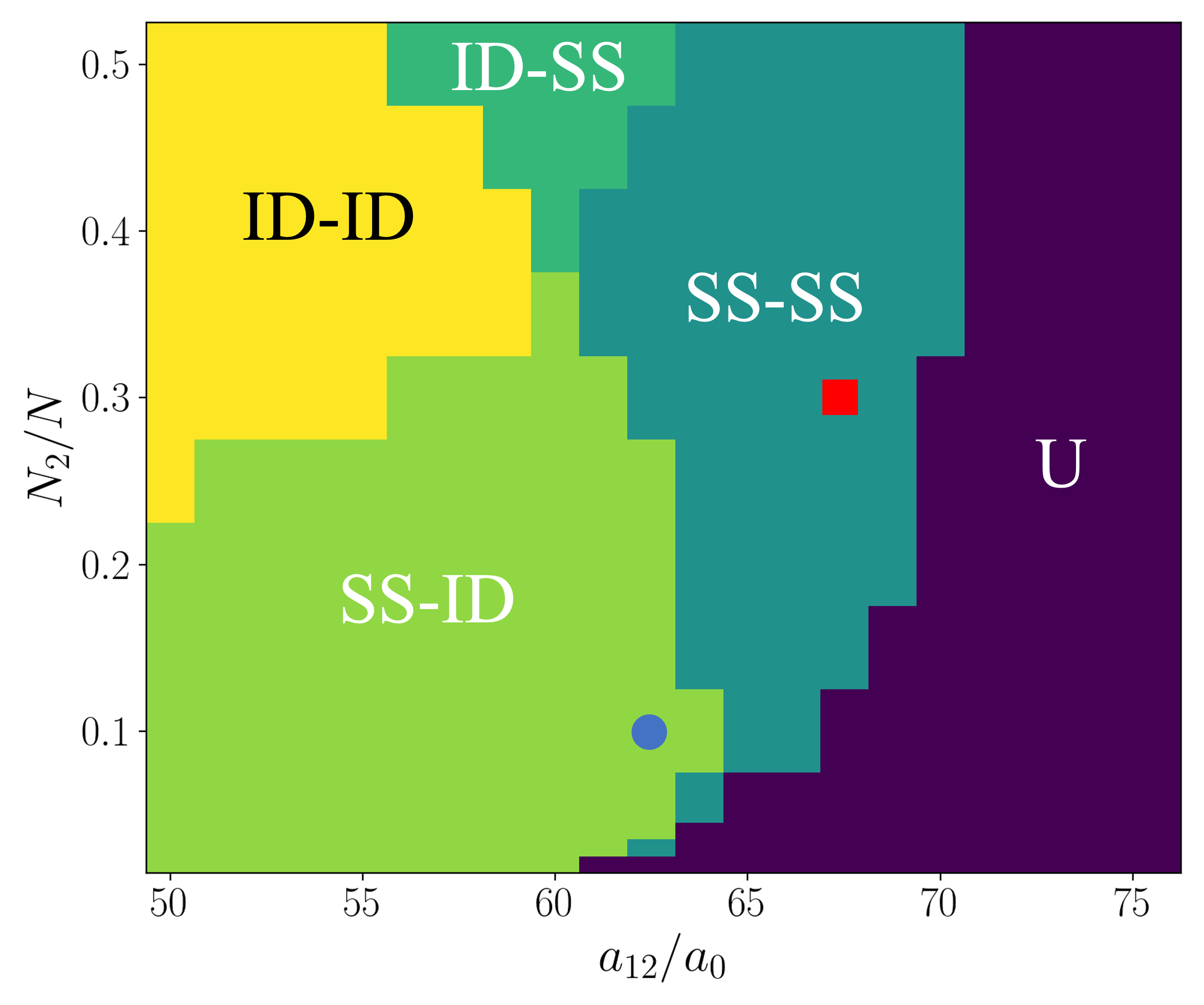
Figure 3: Ground-state phases of the binary mixture as a function of $a_{12}/a_{0}$ and $N_{2}/N$, for the same parameters as Fig. 1. The blue circle and red square indicate the cases of Figs. 1 (b) and (c), respectively.

Effective dipolar strength and local roton instability.–

We introduce at this point a model, that shows that droplet catalyzation is triggered by a roton instability due to the local modification of the effective dipolar strength. The unmodulated mixture presents an approximately constant polarization $n_{2}(\vec{r})/n_{1}(\vec{r})\simeq n_{2}(0)/n_{1}(0)=P$ in the central region in which the density modulation develops at the U-SS transition. This is satisfied well for a balanced mixture, but it remains a fairly good approximation down to the impurity regime footnote-SM . We may then introduce the local-polarization approximation, reducing our analysis to the case of a mixture with constant polarization $P$, where $\psi_{1}(\vec{r})\simeq\frac{1}{\sqrt{1+P}}\psi(\vec{r})$ and $\psi_{2}(\vec{r})\simeq\sqrt{\frac{P}{1+P}}\psi(\vec{r})$. This reduces the problem to a scalar model given by the energy functional:

$$E = \int d^{3}r\left[\psi(\vec{r})^{*}\left(\frac{-\hbar^{2}\nabla^{2}}{2m}+V_{\mathrm{trap}}(\vec{r})\right)\psi(\vec{r})\right\delimiter 00$$ (6)

$$+ \frac{1}{2}g_{\mathrm{eff}}(P)\chi(P)n(\vec{r})^{2}$$

$$+ \left\delimiter 00\frac{3g_{\mathrm{eff}}^{d}(P)}{8\pi}\int d^{3}r^{\prime}U_{dd}(\vec{r}-\vec{r}^{\prime})n(\vec{r}\,^{\prime})n(\vec{r})\right].$$

where $n(\vec{r})=|\psi(\vec{r})|^{2}$, $g_{\mathrm{eff}}(P)=4\pi\hbar^{2}a_{\mathrm{eff}}(P)/m$, and $g_{\mathrm{eff}}^{d}(P)=4\pi\hbar^{2}a_{\mathrm{eff}}^{d}(P)/m$. Note that for the relatively low densities that characterize the U regime, we have included (to a very good approximation footnote-SM ) the LHY contribution to the chemical potential by regularizing $g_{\mathrm{eff}}\to g_{\mathrm{eff}}\chi$, with

$$\chi\!=\!1+\frac{8\sqrt{n_{0}a_{\mathrm{eff}}^{3}}}{3\sqrt{2\pi}}{\cal R}\!\left[\int_{0}^{1}\!\!du\!\!\sum_{\lambda=\pm}\!\left[\frac{V_{\lambda}\left(u,\frac{1}{1+P},\frac{P}{1+P}\right)}{g_{\mathrm{eff}}}\right]^{\frac{5}{2}}\right].$$ (7)

Crucially, the system is characterized by a polarization-dependent effective scattering length $a_{\mathrm{eff}}(P)=\frac{a_{11}+P^{2}a_{22}+2Pa_{12}}{(1+P)^{2}}$, and dipolar length $a_{\mathrm{eff}}^{d}(P)=\frac{a_{11}^{d}+P^{2}a_{22}^{d}+2Pa_{12}^{d}}{(1+P)^{2}}$. As a result the effective dipolar strength $\epsilon_{\mathrm{dd}}=a_{\mathrm{eff}}^{d}/a_{\mathrm{eff}}$ depends on the local polarization. In Fig. 4(a) we depict $\epsilon_{\mathrm{dd}}$ for $P=1$ (which is approximately the central polarization for $N_{2}/N=0.5$ in our calculations), as a function of $a_{12}$. For $a_{12}<85\,a_{0}$ (for the parameters of Fig. 1) the mixture is locally effectively more dipolar than the component 1 alone, i.e. $\epsilon_{\mathrm{dd}}(P=1)>\epsilon_{\mathrm{dd}}(P=0)$. For a sufficiently low $a_{12}$, $\epsilon_{\mathrm{dd}}$ is large enough to drive the system locally unstable, as discussed below.

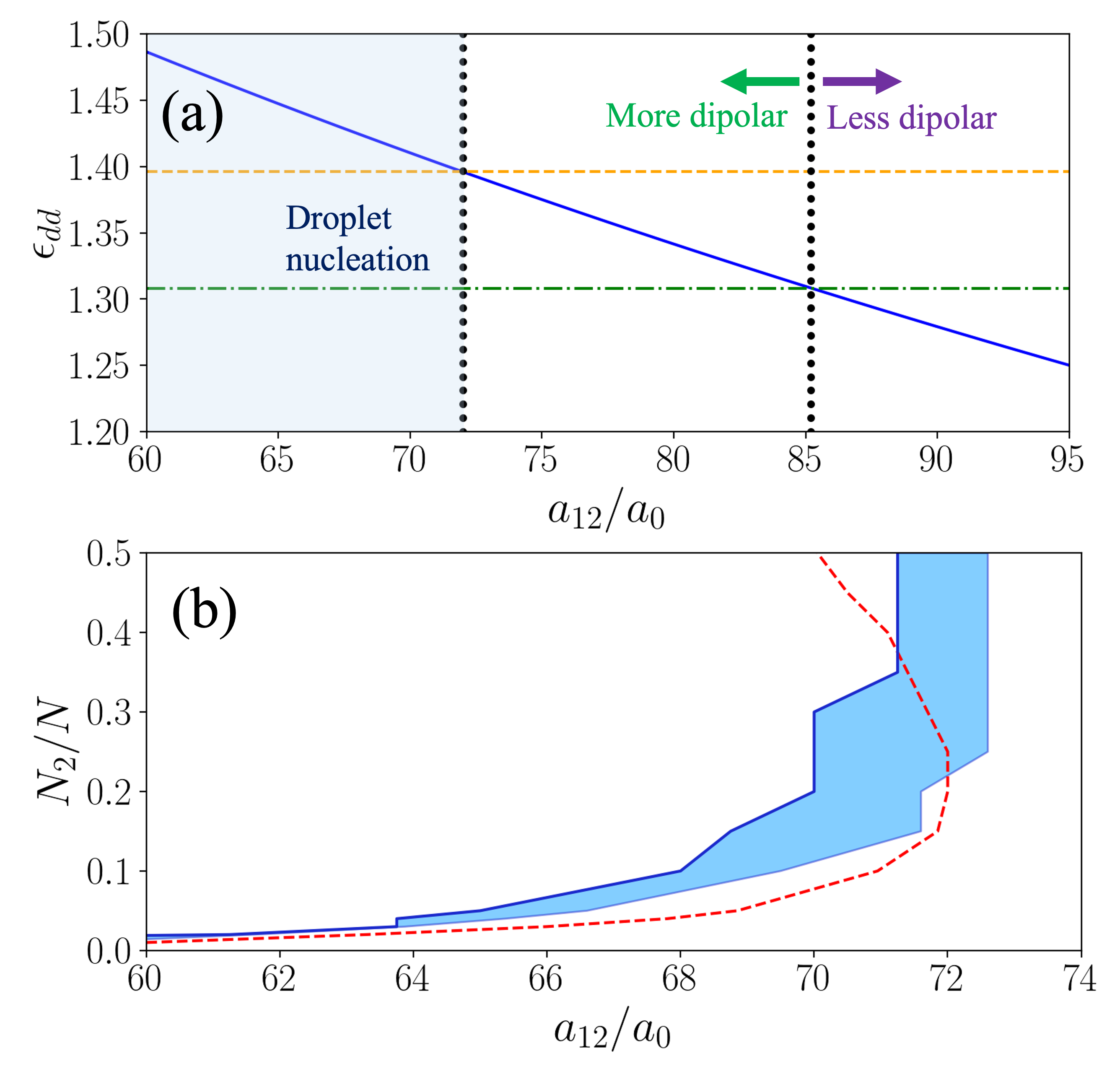
Figure 4: (a) Effective dipolar strength $\epsilon_{\mathrm{dd}}$ (blue-solid curve) for the parameters of Fig. 1 and $P=1$, as a function of $a_{12}$. For $a_{12}<85a_{0}$, $\epsilon_{\mathrm{dd}}(P=1)>\epsilon_{\mathrm{dd}}(P=0)$ (dot-dashed line), and hence the mixture is more dipolar than the component 1 alone. For $a_{12}<72a_{0}$, $\epsilon_{\mathrm{dd}}>1.39$ (dashed line), the value at which droplets start to be nucleated in a single component. (b) Onset of the density modulation. The solid dark-blue curve depicts for a given $N_{2}/N$ the value of $a_{12;cr}$ , such that for $a_{12}<a_{12;cr}$ both components have a non-zero contrast. The blue-shaded area indicates the threshold regime of $a_{12}$ values for which we observe at the trap center the growth of a significant deviation from the unmodulated density profile, although no local density minima have yet developed, and hence the contrast $\cal{C}$ remains zero. The red/solid curve indicates the onset of the central roton-instability as obtained from Eq. (8), using the central density $n_{0}$ and polarization $P$ evaluated in the U regime for $a_{12}=75\,a_{0}$.

Since the condensate is very elongated in the axial direction, we may approximate the density profile of the unmodulated mixture at the axial trap center as $n(\vec{r})\simeq n(y,z)$. Assuming a transversal Thomas-Fermi profile, $n(y,z)\simeq n_{0}\left(1-y^{2}/R_{y}^{2}-z^{2}/R_{z}^{2}\right)$, we may directly employ the formalism developed in Ref. Chomaz2018 for the study of the roton instability in an elongated single-component dipolar condensate footnote-SM . The roton energy $\Delta_{\mathrm{R}}$ acquires the form:

$$\left(\frac{\Delta_{\mathrm{R}}}{g_{\mathrm{eff}}n_{0}}\right)^{2} = \sum_{j=y,z}\Lambda_{j}^{2}f_{j}(\kappa,\epsilon_{\mathrm{dd}})-\frac{4}{9}\left(\epsilon_{\mathrm{dd}}-\chi\right)^{2}$$ (8)

where $\Lambda_{j}=\frac{\hbar\omega_{j}}{g_{\mathrm{eff}}n_{0}}$, $f_{j}(\kappa,\epsilon_{\mathrm{dd}})=\frac{\epsilon_{\mathrm{dd}}(1+\kappa)^{2}/2}{(1+\kappa)^{2}\chi+\epsilon_{\mathrm{dd}}(2+\beta_{j}\kappa-\kappa^{2})}$, $\beta_{y}=-2$, $\beta_{z}=4$, and the transversal aspect ratio $\kappa=R_{z}/R_{y}$ is given by $(\omega_{y}/\omega_{z})^{2}=\kappa^{2}f_{z}(\kappa,\epsilon_{\mathrm{dd}})/f_{y}(\kappa,\epsilon_{\mathrm{dd}})$.

From the eGPE calculations, we obtain $n_{0}=n(0)$ and $P$ for different $N_{2}/N$ and $a_{12}=75\,a_{0}$, in the U regime close to the SS transition. From the condition $\Delta_{\mathrm{R}}=0$, we determine the value of $a_{12}$ that , according to the model above, would result in roton instability at the center of the unmodulated condensate. The results are in very good qualitative agreement (and indeed also quantitative, considering the deviations from both the local-polarization approximation and the transversal Thomas-Fermi profile) with the threshold for droplet nucleation obtained from the coupled eGPEs (Fig. 4(b)). Droplet catalyzation hence results from the roton instability induced by the locally-modified dipolar strength.

Conclusions.–

Doping with a second dipolar component may catalyze droplet nucleation and supersolidity in an otherwise unmodulated dipolar condensate. This stems from the local modification of the effective dipolar strength, which for a sufficiently low value of $a_{12}$ results in a local roton instability, which triggers droplet nucleation, once arrested by quantum stabilization. We note that droplet catalyzation does not require full overlapping of both components, but only an overlapping region with an extension larger than the transversal size of the droplet. Strikingly, catalyzation may be efficient even for a very small doping, well within the impurity regime.

Droplet catalyzation allows for the realization of a two-fluid supersolid, characterized by generally different superfluid fractions in each component. We stress that, although the triggering mechanism behind droplet nucleation may be understood from a locally-valid scalar model (6), the supersolid mixture that forms once droplets nucleate is a genuinely two-component system, and not an effective scalar condensate. The two-fluid supersolid thus constitutes a novel platform for the study of the interplay between density modulation, spin physics, and the different superfluid character of each component. The intriguing properties of two-fluid dipolar supersolids, and in particular their elementary excitations, will be the focus of future research.

 

SUPPLEMENTAL MATERIAL:
"Catalyzation of supersolidity in binary dipolar condensates"

D. Scheiermann,¹ Luis A. Peña Ardila,¹ T. Bland,^2,3 R. N. Bisset³ and L. Santos ¹

¹Institut für Theoretische Physik, Leibniz Universität Hannover, Germany

²Institut für Quantenoptik and Quanteninformation, Innsbruck, Austria

³ Institut für Experimentalphysik, Universität Innsbruck, Austria

In this Supplemental Material, we provide additional examples of the different ground states phases discussed in the main text, and make additional comments on the overall superfluidity and the relative contribution of each component to it. We discuss as well further details concerning the simplified model employed in the main text for the understanding of the droplet catalyzation. Finally, we briefly comment on the possibility of realizing a supersolid of immiscible droplets.

I Change of the density profiles of the components

Figure 3 of the main text shows the possible ground-states of the miscible mixture: U, SS-SS, SS-ID, ID-SS, and ID-ID. In Figs. 1(b) and (c) of the main text we present two cases, in the SS-ID and SS-SS regimes, respectively. In Figs. S1 (a) and (b), we illustrate in more detail the transition experienced by the density profiles as a function of $N_{2}/N$. Figure S1 (a) shows the density profiles of both components for the same parameters as those of Fig. 1 of the main text, for the case of $a_{12}=62.5a_{0}$. For growing $N_{2}/N$ the system transitions from the SS-ID regime to the SS-SS regime and finally into the ID-SS regime. In Fig. S1 (b) we depict the density profiles of both components for the same case but with $a_{12}=67.5a_{0}$. For growing $N_{2}/N$ the system transitions from the U regime into the SS-SS regime.

Concerning our numerical calculations, we have solved the coupled eGPE equations using standard split-operator and fast-Fourier transformation techniques. We employ in the calculations shown in the paper numerical boxes $|x|<12l_{x}$, $|y|<6l_{x}$, $|z|<6l_{x}$, with $l_{x}=\sqrt{\hbar/m\omega_{x}}=1.36\,\mu\mathrm{m}$, and a number of points $N_{x,y,z}=128,64,32$. We have checked that increasing the boxes and/or the number of points does not change appreciably our results.

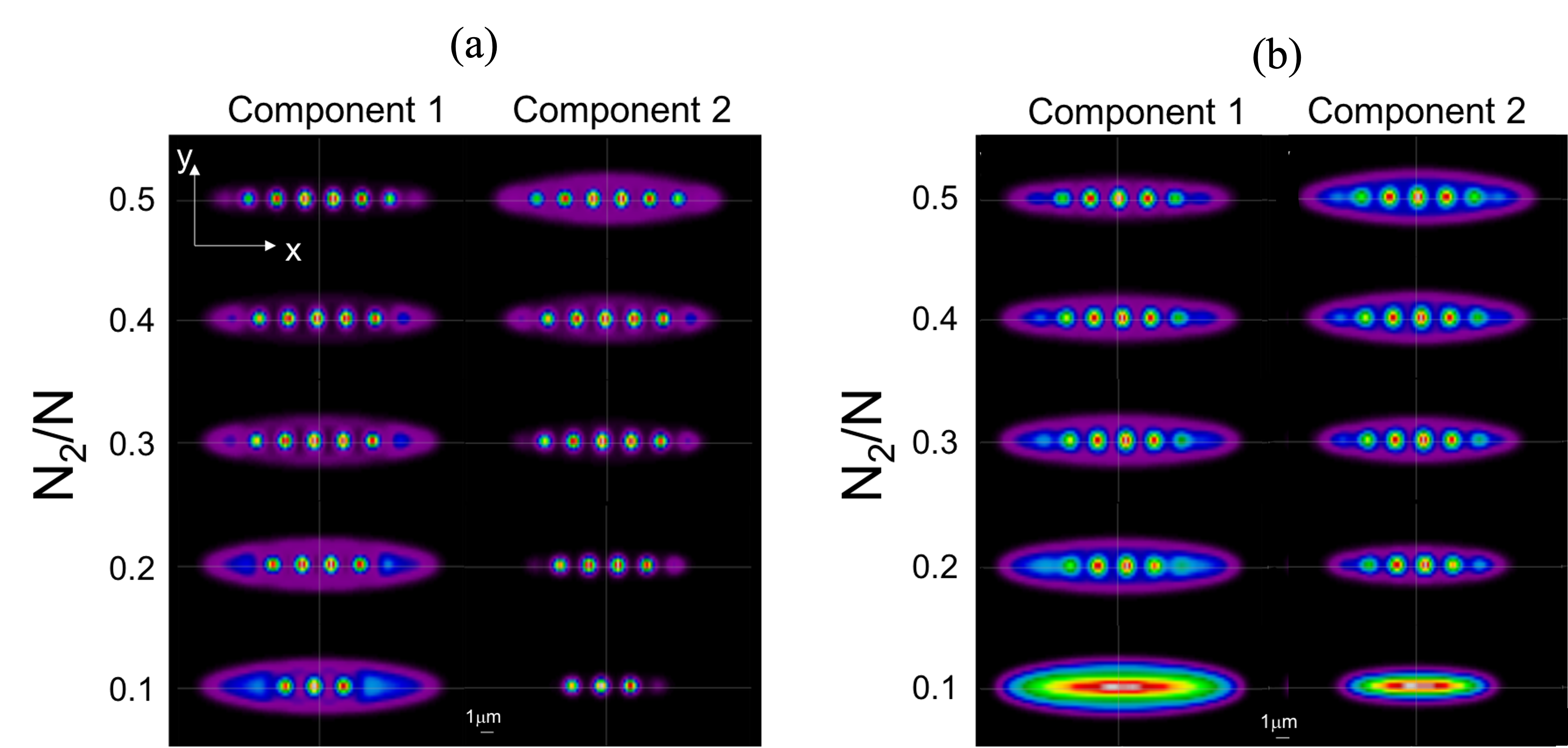
Figure S1: (a) Binary mixture with $N=63000$, $\omega_{x,y,z}=2\pi(33,110,167)\,\mathrm{Hz}$, $\mu_{1}=10\mu_{B}$, $\mu_{2}=9\mu_{B}$, $a_{11}=a_{22}=100a_{0}$ and $a_{12}=62.5a_{0}$. (b) Same but with $a_{12}=67.5a_{0}$

II Overall superfluidity

As mentioned in the main text, the overall superfluid fraction $f_{s}=\frac{N_{1}}{N}f_{s}^{(1)}+\frac{N_{2}}{N}f_{s}^{(2)}$ (see Fig. S2 (a)), characterizes the reduction of the momentum of inertia (compared to its classical value) as would be measured e.g. from the response of the mixture to a spin-independent scissors-like perturbation. The relative contribution of each component to the overall superfluid fraction may be evaluated from the relative superfluid fraction (see Fig. S2 (b)): $f_{s}^{(rel)}=\frac{1}{f_{s}}\left(\frac{N_{1}}{N}f_{s}^{(1)}-\frac{N_{2}}{N}f_{s}^{(2)}\right)$. In accordance to Fig. 3 of the main text, we see that in addition to the U and ID-ID regimes, there is an intermediate regime with finite overall contrast and superfluidity. Note that whereas for low $N_{2}/N$ the superfluidity is dominated by the first component, the situation reverses when $N_{2}/N$ approaches $0.5$. In the region we denote as SS-ID (ID-SS) in Fig. 3 of the main text, superfluidity is given only by component 1 (2).

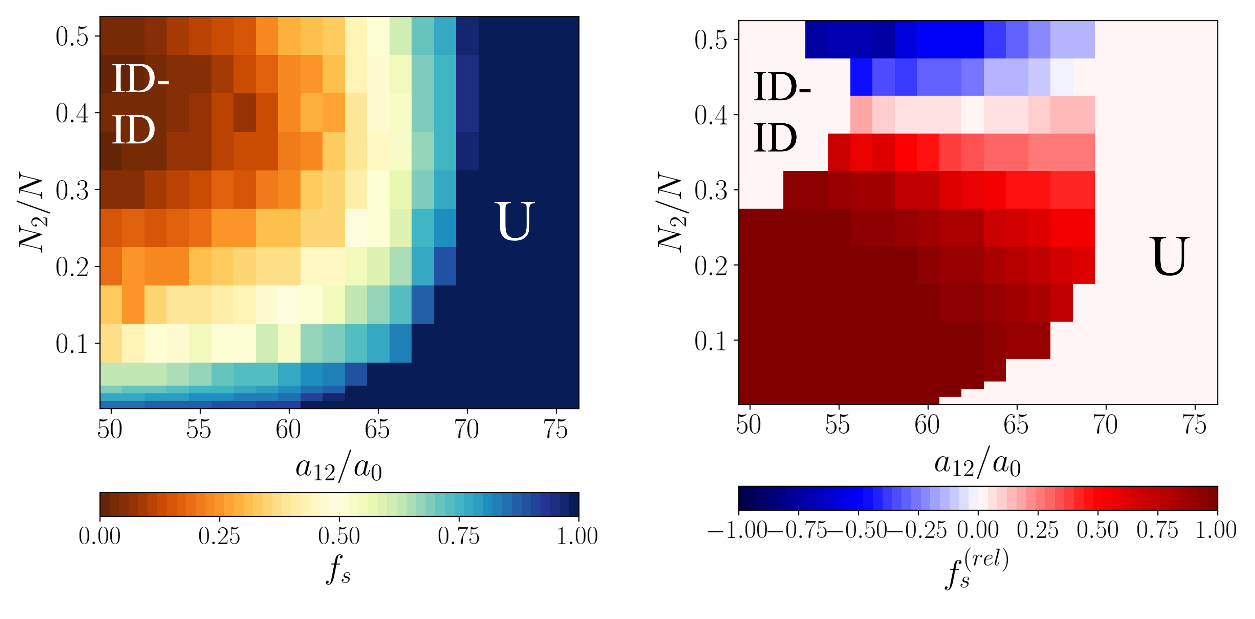
Figure S2: Overall superfluid fraction $f_{s}$ (a) and relative fraction $f_{s}^{(rel)}$ (b) for the same parameters as Fig. 2 of the main text. In Fig. (b) we have excluded the U and ID-ID regions. Note that for growing $N_{2}/N$ the superfluidity transitions from being dominated by the first component to be dominated by the second one. In the SS-ID (ID-SS) phase the superfluidty is to a good approximation only given by component 1 (2).

III Evaluation of the local roton instability

In this section we provide additional details concerning the model employed in the main text for the study of the local roton instability that induces the observed droplet catalyzation.

III.1 Validity of the local polarization approximation

The model discussed in the main text employs the fact that at the trap center, in the region where the density modulation develops, the polarization is approximately constant. This is satisfied well in the balanced mixture case, $N_{1}=N_{2}$ (see Fig. S3(a)), were the two components have very similar density profiles, and indeed the mixture can be well understood using single-mode approximation in the whole cloud Smith2021b . In contrast, single-mode approximation obviously fails in the impurity regime, since the minority component moves into the central region of the majority component. However, even in that case, the polarization remains approximately constant in the central region where a droplet develops (see Fig. S3(b)).

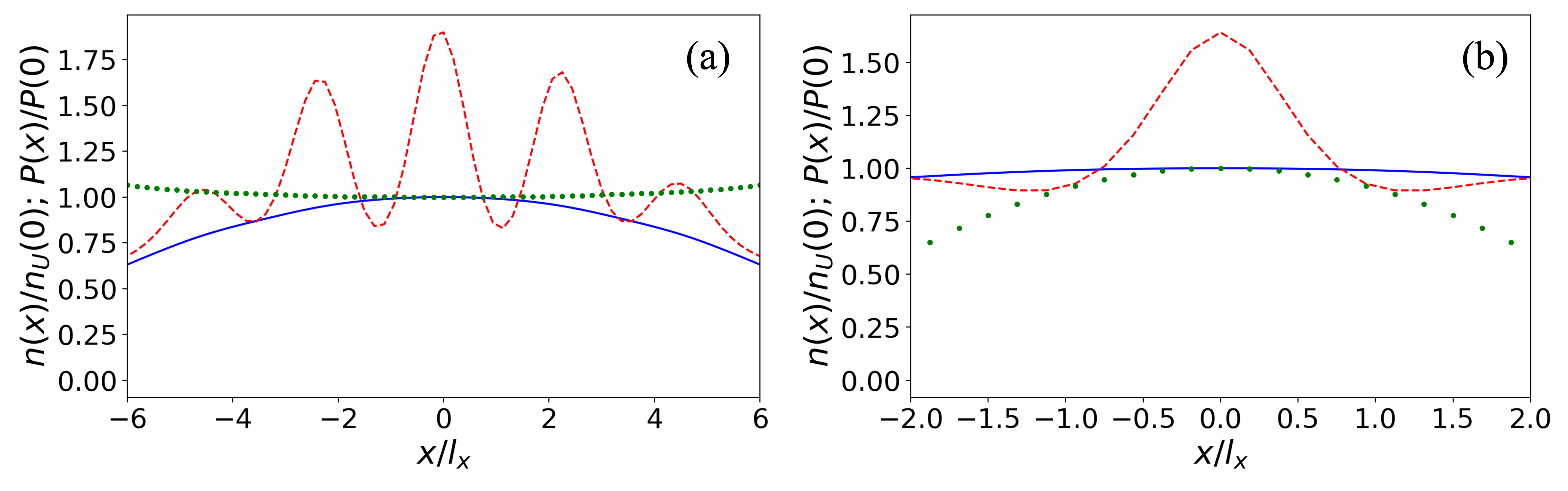
Figure S3: (a) Central region where droplets develop. We consider the same parameters as in Fig. 1 of the main text. Figure (a) depicts the case of a balanced mixture ($N_{2}/N=0.5$). The solid-blue and dashed-red curve indicate the density $n_{1}(x,0,0)$ for $a_{12}=75a_{0}$ (unmodulated regime) and $a_{12}=70a_{0}$ (modulated regime), respectively, whereas the dotted-green curve depicts the polarization $P=n_{2}(x,0,0)/n_{1}(x,0,0)$. Figure (b) shows the case of a very imbalanced mixture ($N_{2}/N=0.05$). The solid-blue and dashed-red curve indicate the density $n_{1}(x,0,0)$ for $a_{12}=66.25a_{0}$ (unmodulated regime) and $a_{12}=57.5a_{0}$ (modulated regime), respectively, whereas the dotted-green curve depicts the polarization $P=n_{2}(x,0,0)/n_{1}(x,0,0)$. In both figures, the length unit is $l_{x}=\sqrt{\hbar/m\omega_{x}}$, and we have normalized the density by the central value $n_{U}(0)$ of the density of the unmodulated case, and the polarization by its central value $P(0)$.

III.2 Regularization of the contact term

Assuming a constant polarization $P$, we re-express $n_{1}=\frac{n}{1+P}$ and $n_{2}=\frac{nP}{1+P}$, with $P=n_{2}/n_{1}$ and $n=n_{1}+n_{2}$. We may then rewrite the contribution of the contact interactions and the LHY to the energy functional of Eq. (3) of the main text in the form:

$$E_{\mathrm{SR}+\mathrm{LHY}}(\vec{r})=\frac{1}{2}g_{\mathrm{eff}}(P)n(\vec{r})^{2}+\xi_{\mathrm{LHY}}\left(\frac{1}{1+P},\frac{P}{1+P}\right)n(\vec{r})^{5/2}.$$ (S1)

The contribution to the effective extended Gross-Pitaevskii equation for $\psi(\vec{r})$ will be given by the local chemical potential:

$$\mu_{\mathrm{SR}+\mathrm{LHY}}(\vec{r})=g_{\mathrm{eff}}(P)n(\vec{r})+\frac{5}{2}\xi_{\mathrm{LHY}}\left(\frac{1}{1+P},\frac{P}{1+P}\right)n(\vec{r})^{3/2}.$$ (S2)

As shown in Fig. S4, this expression may be well approximated by:

$$\mu_{\mathrm{SR}+\mathrm{LHY}}(\vec{r})\simeq g_{\mathrm{eff}}(P)\chi(P)n(\vec{r})$$ (S3)

with

$$\chi(P)=1+\frac{5}{2}n_{0}^{1/2}\frac{\xi_{\mathrm{LHY}}\left(\frac{1}{1+P},\frac{P}{1+P}\right)}{g_{\mathrm{eff}}(P)}=1+\frac{8}{3\sqrt{2\pi}}\sqrt{n_{0}a_{\mathrm{eff}}^{3}(P)}\,\,{\cal R}\!\left[\int_{0}^{1}du\sum_{\lambda=\pm}\left(\frac{V_{\lambda}\left(u,\frac{1}{1+P},\frac{P}{1+P}\right)}{g_{\mathrm{eff}}(P)}\right)^{5/2}\right]$$ (S4)

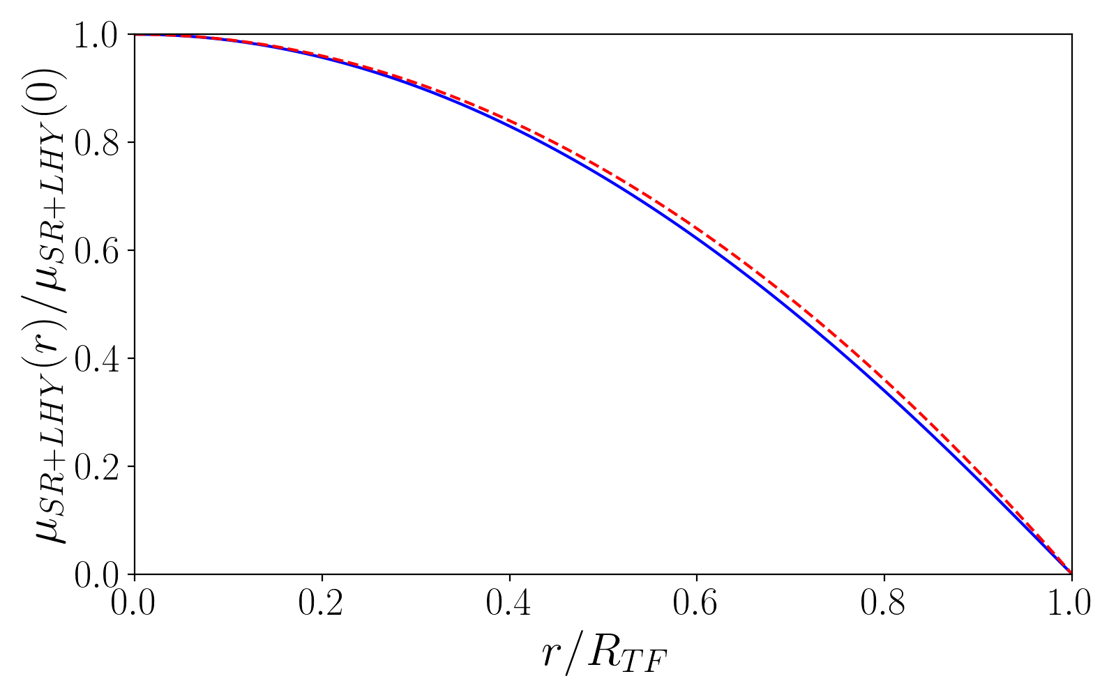
Figure S4: Comparison of $\mu_{SR+LHY}[n(r)]$ (solid, blue) and the approximate $g_{\mathrm{eff}}\chi(P)n(r)$ (dashed, red) for a one-dimensional Thomas-Fermi profile $n(r)=n_{0}\left(1-r^{2}/R_{\mathrm{TF}}^{2}\right)$. We have employed a density $n_{0}=5\times 10^{20}\mathrm{m}^{-3}$, and Dy atoms with $a_{11}=a_{22}=100a_{0}$, $a_{12}=70a_{0}$, $\mu_{1}=10\mu_{B}$, and $\mu_{2}=9\mu_{B}$, and polarization $P=1$.

III.3 Transversal Thomas-Fermi profile

Assuming an axially-homogeneous condensate, with a transversal Thomas-Fermi profile, $n=n_{0}(1-y^{2}/R_{y}^{2}-z^{2}/R_{z}^{2})$, we may proceed as in Refs. Eberlein2005 ; Chomaz2018 to determine the transversal Thomas-Fermi radii:

$$R_{y}^{2} = \frac{2g_{\mathrm{eff}}(P)?n_{0}}{m\omega_{y}^{2}}\left[\chi(P)+\epsilon_{\mathrm{dd}}(P)\left(\frac{2-2\kappa-\kappa^{2}}{(1+\kappa)^{2}}\right)\right],$$ (S5)

$$R_{z}^{2} = \frac{2g_{\mathrm{eff}}(P)?n_{0}}{m\omega_{z}^{2}}\left[\chi(P)+\epsilon_{\mathrm{dd}}(P)\left(\frac{2+4\kappa-\kappa^{2}}{(1+\kappa)^{2}}\right)\right],$$ (S6)

with $\kappa=R_{z}/R_{y}$, given by the relation:

$$\left(\frac{\omega_{y}}{\omega_{z}}\right)^{2}=\kappa^{2}\left[\frac{\chi(P)+\epsilon_{\mathrm{dd}}(P)\left(\frac{2-2\kappa-\kappa^{2}}{(1+\kappa)^{2}}\right)}{\chi(P)+\epsilon_{\mathrm{dd}}(P)\left(\frac{2+4\kappa-\kappa^{2}}{(1+\kappa)^{2}}\right)}\right]$$ (S7)

III.4 Roton energy

Using the procedure outlined in the Suppl. Material of Ref. Chomaz2018 , we may determine the excitation spectrum in the vicinity of the roton minimum (see Eq. (1) in Ref. Chomaz2018 ):

$$\xi(k_{x})^{2}\simeq\Delta_{\mathrm{R}}^{2}+\frac{2\hbar^{2}k_{\mathrm{R}}^{2}}{m}\frac{\hbar^{2}}{2m}\left(k_{x}-k_{\mathrm{R}}\right)^{2},$$ (S8)

where $k_{\mathrm{R}}$ is the roton momentum and

$$\Delta_{\mathrm{R}}^{2}=2g_{\mathrm{eff}}n_{0}\epsilon_{\mathrm{dd}}\frac{\hbar^{2}}{2m}\left(\frac{1}{R_{y}^{2}}+\frac{1}{R_{z}^{2}}\right)-\frac{4}{9}\left(g_{\mathrm{eff}}(P)n_{0}\right)^{2}\left(\epsilon_{\mathrm{dd}}-\chi(P)\right)^{2}.$$ (S9)

Using Eqs. (S5) and (S6), we recover the expression of Eq. (8) of the main text.

IV Supersolids of immiscible droplets.

In the main text, we have only focused on the miscible regime. When $a_{12}>0$ increases, inter-component repulsion eventually leads to immiscibility, i.e. to the spatial separation of the components. In a non-dipolar gas, immiscibility would result, for the elongated geometry considered, in phase separation along the trap axis for a sufficiently large $a_{12}$. This is observed as well when extending the regimes of Figs. 2 and 3 of the main text into larger $a_{12}$ values. A dipolar mixture may open, however, more intriguing scenarios. We briefly illustrate in the following one of these scenarios.

Recent studies Smith2021 ; Bisset2021 have shown that dipolar mixtures allow for immiscible self-bound droplets, in which one of the components is attached, along the dipole axis, to the ends of a droplet of the second component. This attachment results from the formation at those locations of energy minima induced by the inter-component dipole-dipole interaction. Interestingly, immiscible dipolar mixtures may form a supersolid array of these immiscible droplets. This is in particular the case if $a_{22}$ is low-enough, such that the second component alone would nucleate droplets. This is illustrated in Fig. S5, where we depict the ground-state densities for $a_{11}=95a_{0}$, $a_{22}=76a_{0}$, and $a_{12}=84a_{0}$, and $N_{2}/N=0.5$. Note the formation of immiscible droplets, similar as those discussed in Refs. Bisset2021 ; Smith2021 ; Smith2021b , which arrange in a peculiar double supersolid.

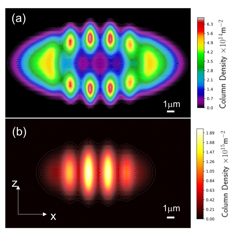
Figure S5: Supersolid of immiscible droplets. Column density on the $xz$ plane for the component 1 (a) and 2 (b) for $N=63000$, $(\omega_{x},\omega_{y},\omega_{z})=(2\pi(33,110,167)$Hz, $N_{2}/N=0.5$, $a_{11}=95a_{0}$, $a_{22}=76a_{0}$, and $a_{12}=84a_{0}$.

References

- (1) J. C. Smith, P. B. Blakie, and D. Baillie, Phys. Rev. A 104, 053316 (2021).
- (2) C. Eberlein, S. Giovanazzi, and D. H. J. O’Dell, Phys. Rev. A 71, 033618 (2005).
- (3) L. Chomaz, R. M. W. van Bijnen, D. Petter, G. Faraoni, S. Baier, J. H. Becher, M. J. Mark, F. Wächtler, L. Santos, and F. Ferlaino, Nature Phys. 14, 442 (2018).
- (4) R. N. Bisset, L. A. Peña Ardila, and L. Santos, Phys. Rev. Lett. 126, 025301 (2021).
- (5) J. C. Smith, D. Baillie, and P. B. Blakie, Phys. Rev. Lett. 126, 025302 (2021).