Emergent conformational properties of end-tailored transversely propelling polymers

Abstract

We study the dynamics and conformations of a single active semiflexible polymer whose monomers experience a propulsion force perpendicular to the local tangent, with the end beads being different from the inner beads (“end-tailored”). Using Langevin simulations, we demonstrate that, apart from sideways motion, the relative propulsion strength between the end beads and the polymer backbone significantly changes the conformational properties of the polymers as a function of bending stiffness, end-tailoring and propulsion force. Expectedly, for slower ends the polymer curves away from the moving direction, while faster ends lead to opposite curving, in both cases slightly reducing the center of mass velocity compared to a straight fiber. Interestingly, for faster end beads there is a rich and dynamic morphology diagram: the polymer ends may get folded together to 2D loops or hairpin-like conformations that rotate due to their asymmetry in shape and periodic flapping motion around a rather straight state during full propulsion is also possible. We rationalize the simulations using scaling and kinematic arguments and present the state diagram of the conformations. Sideways propelled fibers comprise a rather unexplored and versatile class of self-propellers, and their study will open novel ways for designing, e.g. motile actuators or mixers in soft robotics.

I Introduction

Self-propelled particles are the most studied realisation of active matter Gompper et al. (2020), i.e. systems in out-of-equilibrium states using energy sources or fluxes to perform tasks, in this case to move in an autonomous and persistent fashion. Prominent examples from the living world are swimming ciliated bacteria Berg and Anderson (1973); Lauga and Powers (2009) gliding myxobacteria Mauriello et al. (2010); Peruani et al. (2012) and cytoskeletal filaments transported on motor carpets Ray et al. (1993); Schaller et al. (2010)In the last 15 years a variety of artificial self-propellers has been developed, mostly microswimmers, with elegant examples being catalytic nanorods Paxton et al. (2004) and phoretically or demixing-driven colloidal Janus particles Ebbens et al. (2012); Howse et al. (2007); Soto and Golestanian (2014); Buttinoni et al. (2012).

Most self-propellers studied so far are either spherical or the propulsion direction is associated with the major body axis. However, recently also sideways propelled objects have been developed. In the colloidal realm, examples are sideways propelling short ellipsoids Tierno et al. (2010) and cylinders Vutukuri et al. (2016) as well as straight and bent Janus micro-rods Rao et al. (2019) and 3D printed helical or more complex shapes Doherty et al. (2020). Active Janus beads were recently assembled to flexible chains in an electric field Vutukuri et al. (2017), but so far only in staggered orientation with no sideways propulsion. Other examples are anisotropic rollers, for instance flexible fibers propelled by a flux of heat or swelling agent to roll along their long axis Baumann et al. (2018); Bazir et al. (2020) as well as light-driven rolling helices and spring actuators Jiang et al. (2021).

While most active colloidal systems are mechanically rigid so far, it is evident that a certain deformability of active objects will lead to more complex behavior with possible applications in soft robotics Yan et al. (2016). Minimal models of active polymers, composed of stresslets or propelled beads, were shown to exhibit translational or rotational motion or spiraling Jayaraman et al. (2012); Isele-Holder et al. (2015); Eisenstecken et al. (2016); Jiang and Hou (2014).

While tangentially propelled polymers typically deform only weakly, as the main force is along the backbone, it is clear that for transversely propelled slender objects, deformations can easily be excited – similar to but different from fibers sedimenting or actively dragged through a viscous environment Lagomarsino et al. (2005); Xu and Nadim (1994); Schlagberger and Netz (2005); Marchetti et al. (2019) – and in turn will interfere with the propulsion. Motivated by this reasoning we here study the following principal questions: What is the interplay of active forces and flexibility in a sideways propelled slender object? And can one tailor the properties to dynamically obtain certain shapes or even complex behavior that may be useful to perform certain tasks? To answer these questions we propose and study a simple coarse-grained active polymer model with two main ingredients: first, the (local) propulsion force is pointing in the direction normal to the (local) backbone direction. And second, we consider what we call “end-tailoring”, i.e. the end beads are made different from the backbone beads, which upon self-propulsion will induce an initial bending deformation and, depending on parameters and design, complex behavior.

The work is organized as follows. Sec. II introduces the coarse-grained model for an end-tailored semi-flexible filament subject to active forces perpendicular to its contour. In Sec. III, we briefly discuss the propulsion behavior without end-tailoring. Sec. IV studies the case of slower end beads where we extensively analyze the propulsion induced bending and its feedback on velocity. Sec. V studies the case of faster end beads, where the behaviour turns out to be much richer, leading to closed shapes and even periodic flapping during propulsion. Finally, in Sec. VI we summarize our main findings and comment on future directions.

II Model and computational details

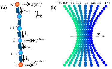
Figure 1: (a) Schematic of the model for a transversely propelling end-tailored filament. Briefly, bead $i$ gets sideways active force contributions from the tangents ${\bf t}_{i}$ and ${\bf t}_{i-1}$, whereas the end beads $1$ and $N$ get the propulsion force only from the tangents ${\bf t}_{1}$ and ${\bf t}_{N-1}$, respectively. More importantly, while all inner beads (blue) have the same absolute value of propulsion force $|{\bf F}_{i}^{active}|=f_{p}$, the end beads (red) experience a smaller (parameter $\alpha<1$) or larger (parameter $\alpha>1$) propulsion force $\alpha f_{p}$. (b) Conformations of steadily propelling polymers for various values of $\alpha$. For $\alpha=1$ the polymer is straight (in the absence of noise), end-tailored propulsion induces curving. The propulsion direction is indicated by the arrow and $\mathbf{v}$. Parameters: bending stiffness $\kappa=2$, $f_{p}=2$ and $\alpha$ as indicated.

We model a two-dimensional (2D) semiflexible polymer, consisting of $N$ beads of diameter $\sigma$ and mass $m_{i}=m$ with coordinates ${\bf r}_{i}$ $(i=1,...,N)$. The advantage of employing a polymeric model is that one can easily tune both the aspect ratio (via the length) and the stiffness of the object. An active propulsion force that is perpendicular to the local tangent along the polymer contour is implemented as explained below. In the stiff limit, the model corresponds to a transversely propelled rod, but when the polymer curves by the prevalent forces, complex behaviour is anticipated from the interplay of propulsion and shape. A schematic of the model is given in Fig. 1a.

The time evolution of a monomer is given by the following Langevin equation,

$$m_{i}\frac{d{\bf v}_{i}}{dt}={\bf F}^{poly}_{i}+{\bf F}_{i}^{fric}+{\bf F}_{i}^{noise}+{\bf F}_{i}^{active},$$ (1)

with ${\bf v}_{i}=\frac{d{\bf r}_{i}}{dt}$ the velocity of bead $i$ and the forces on the right hand side being a conservative force modeling the polymeric structure, a friction force, a stochastic force and the active propulsion force.

The conservative force ${\bf F}^{poly}_{i}=-\frac{\partial U(r)}{\partial r_{i}}{\mathbf{\hat{r}}_{ij}}$, where $r=\left|\mathbf{r}_{ij}\right|=\left|\mathbf{r}_{i}-\mathbf{r}_{j}\right|$ is the distance between two beads (and ${\mathbf{\hat{r}}}_{ij}=\mathbf{r}_{ij}/r$), follows the potential $U(r)=U_{WCA}+U_{s}+U_{b}$. Excluded volume interactions between the beads are modeled via the Weeks-Chandler-Anderson potential Weeks et al. (1971),

$$U_{WCA}=4\epsilon\left[\left(\frac{\sigma}{r}\right)^{12}-\left(\frac{\sigma}{r}\right)^{6}+\frac{1}{4}\right],$$ (2)

which vanishes beyond distances greater than $2^{1/6}\sigma$. Here $\epsilon$ measures the strength of the steric repulsion, $\sigma$ is the size of the bead, and both are set to $1$ in the following. This scaling of energy in terms of $\epsilon$ and length in terms of $\sigma$ implies the reduced unit of time $\tau=\sqrt{\frac{m\sigma^{2}}{\epsilon}}$.

Every connected bead in a polymer interacts via a two-body harmonic potential Kremer and Grest (1990),

$$U_{s}=k_{b}\big{(}r-R_{0}\big{)}^{2}.$$ (3)

Here $R_{0}=\sigma$ is the maximum bond length and $k_{b}=4000\epsilon/\sigma^{2}$ is the bond stiffness (this large value making the chain effectively inextensible). These parameters ensure the bond length to be $b\simeq\sigma$ and the polymer contour length to be $L\simeq(N-1)\sigma$ to very good approximation. The three-body bending potential $U_{b}$ is employed for every consecutive triplet of monomers $i$, $i+1$, $i+2$,

$$U_{b}=\kappa\big{(}\theta-\theta_{0}\big{)}^{2}.$$ (4)

It measures the energy cost for departures of the angle $\theta$ between consecutive bond vectors, $\theta=\arccos({\bf\hat{r}}_{i,i+1}\cdot{\bf\hat{r}}_{i+2,i+1})$, from its equilibrium value $\theta_{0}=\pi$. Here $\kappa$ is the bending stiffness, related to the continuum bending stiffness, $\tilde{\kappa}$, via $\kappa=\tilde{\kappa}/2\sigma$.

${\bf F}_{i}^{fric}=-\xi{\bf v}_{i}$ accounts for the frictional force with coefficient $\xi$, which is set to $1$ unless otherwise specified. Note that for simplicity we use an isotropic friction here, but it would be straightforward to implement anisotropic friction (e.g. for hydrodynamic systems). The stochastic (in principle not necessarily thermal) force, ${\bf F}^{noise}_{i}$, is modelled as a white noise with zero mean and variance $4k_{B}T\xi/\Delta t$. In most of our simulation the strength of the noise is zero (deterministic limit), unless otherwise specified.

Finally, we implement an active propulsion force as follows : all the beads of the backbone $(i=2,...,N-1)$ experience the force

$${\bf F}_{i}^{active}=\hat{\bf z}\times\frac{\hat{\bf t}_{i}+\hat{\bf t}_{i-1}}{2}{f_{p}},$$ (5)

Here $\hat{\bf t}_{i}=\frac{{\bf r}_{i}-{\bf r}_{i+1}}{|{\bf r}_{i}-{\bf r}_{i+1}|}$ is the local tangent between beads $i$ and $i+1$. Hence both neighbours of bead $i$ contribute equally, and the respective tangents are averaged. $\hat{\bf z}$ is the unit vector normal to the 2D plane of motion, the cross product defining the normal vector to the contour. $f_{p}$ is the propulsion strength. The active force defined by Eq. 5 is hence distributed equally between the beads and acts perpendicular to the contour of the polymer.

As the end beads $i=1$ and $i=N$ have only one nearest neighbour, we define their active forces as

$${\bf F}_{1}^{active}=\hat{\bf z}\times\hat{\bf t}_{1}\alpha f_{p}\;\;\,\,,\,\,\;\;{\bf F}_{N}^{active}=\hat{\bf z}\times\hat{\bf t}_{N-1}\alpha f_{p},$$ (6)

where in addition, we introduced the parameter $\alpha$. This parameter implements the end-tailoring of the polymer, i.e. differences in the propulsion and/or material properties of the ends, and will play a key role in the emergence of complex shapes during propulsion. Clearly, $\alpha=1$ corresponds to homogeneous propulsion, where one expects – in the absence of noise and after having attained a straight conformation from a given initial condition – a center of mass (c.o.m.) velocity of $V=v_{cm}=f_{p}/\xi$. In case $\alpha<1$ ($>1$), the end beads move slower (faster), inducing curving while propelling as shown in Fig. 1b. For higher propulsion strengths more complex conformational dynamics emerges as investigated in the following.

The effect of a different propulsion of the ends, modelled here by the parameter $\alpha$, should always be present in a real system, since the ends are typically slightly different from the bulk. However, this is not very generic and typically a weak and subtle effect. To experimentally realize large deviations from $\alpha=1$, it is best to tailor the ends specifically. Consider a chain of Janus colloids, similar as developed in Vutukuri et al. (2017), but not with a staggered but with a polarized orientation of the beads. Then using colloids with less catalytic activity at the ends will induce a well-defined end-tailoring $\alpha<1$. Conversely, $\alpha>1$ can be achieved for end colloids having larger catalytic activty. In an even simpler fashion, the case $\alpha\simeq 0$ can be achieved by putting passive loads at the ends.

Concerning parameter ranges, in the following we vary the number of beads in the polymer between $N\in\{5,10,25,50\}$, the filament stiffness $\kappa=1-500$, the magnitude of the active force $f_{p}=0.01-30$ and $\alpha=0.05-2$. The parameters can be combined to a dimensionless number, $B=\frac{f_{p}L^{3}}{\sigma^{2}\kappa}$ (note that $\sigma=1$), which characterizes the ratio of (bulk) propulsion to bending rigidity. For all numerical results shown in the following, the equation of motion, Eq. 1, was integrated using LAMMPS Plimpton (1995), with time step $\Delta t=10^{-4}\tau$.

III Homogeneous transversely propelled fiber ($\alpha=1$)

We first study the case of a homogeneously propelled fiber, i.e. $\alpha=1$. Directed vs. diffusive motion can be quantified by the mean squared displacement of the center of mass of the filament, $\rm{MSD}=\Big{\langle}\Big{(}{\bf r}_{cm}(t+\tau)-{\bf r}_{cm}(t)\Big{)}^{2}\Big{\rangle}$, as a function of time. In the absence of noise, one expects all monomers to move with the same propulsion force, leading to a translational motion perpendicular to the long body axis with center of mass (c.o.m.) velocity ${\bf v}_{cm}=f_{p}/\xi$. Such a ballistic dependence on time proportional to the strength of the propulsion force is a hallmark of active propulsion and is clearly visible in Fig. 2a in the absence of noise. Introducing noise changes only weakly the conformation of a stiff polymer (see also the next section), but it induces long-time orientational decorrelation of the whole object. This is shown in Fig. 2b for stiff sideways propelled filaments in the presence of noise ($k_{B}T=1$).

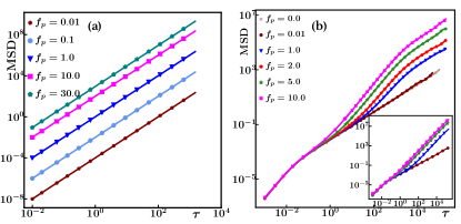
Figure 2: The mean squared displacements ($\rm{MSD}$) of transversely propelled polymers for different propulsion strengths. (a) Perfect self-propulsion without noise, the solid line representing $(f_{p}\tau/\xi)^{2}$. Parameters: $N=25$, $\kappa=100$, $\xi=1$. (b) The case with noise present. The MSD displays up to four regimes; see main text. Parameters: $N=5$, $\kappa=100$, $\xi=100$, $k_{B}T=1$. The inset is for a longer polymer, $N=25,\kappa=500$.

Note that this behavior is similar to what is observed for tangentially propelled objects (or active point particles). As Fig. 2b exemplifies for short filaments $(N=5)$ and high friction $(\xi=100)$, the MSD exhibits four power-law regimes for sufficiently high propulsion strength: a short-time inertial regime, an intermediate diffusive, an active ballistic and a long-time diffusive regime. These regimes are well understood within the Langevin theory of active Brownian motion Howse et al. (2007); Golestanian (2009); Schol et al. (2018). The cross-over time between the initial inertial ballistic and the primary diffusive behaviour is $\sim m/\xi$, independent of propulsion force. The extent of the short-time diffusive regime depends on the active force as the diffusive to active ballistic transition occurs at $\sim D/(2V^{2})$ Schol et al. (2018), with $D=\frac{k_{B}T}{\xi}$ the diffusion coefficient and $V$ the c.o.m. velocity. Directed motion dominates in the third regime and the MSD yields a superdiffusive behaviour (approximately ballistic, ${\rm MSD}\propto t^{2}$). Finally, a long time diffusive regime is attained, due to the decorrelation of the orientation, with an enhanced diffusion coefficient. This occurs at time $\sim D_{r}^{-1}$ Howse et al. (2007); Golestanian (2009); Schol et al. (2018) (with $D_{r}$ the rotational diffusion coefficient) being the time scale at which the object loses its memory of the initial orientation. For a stiff polymer this time rapidly increases with length, $\sim$ $\frac{\xi L^{3}}{k_{B}T}$ Doi and Edwards (1986). In fact, the inset of Fig. 2b shows the case of $N=25$, where the long time diffusive regime is difficult to attain in our simulations.

From Fig. 2b, it is clear that the propulsion force has to be substantial to see the intermediate, self-propelled regime. While the interplay of weak noise-induced bending and propulsion may be interesting, we focus here on the opposite limit, i.e. strong propulsion where the noise is rather irrelevant. Except if otherwise stated, the rest of the paper focuses on the deterministic dynamics without noise.

IV Slower end beads ($\alpha<1$)

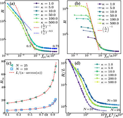
Figure 3: Curvature effects for $\alpha<1$. (a) Radius of curvature $R$ as a function of $f_{p}/\kappa$ in the absence of noise, for length $N=25$ and two different values of $\alpha$. For a given $\alpha$, the curves collapse with two different scaling regimes and a saturation regime. (b) In the presence of noise ($k_{B}T=0.01$) the first scaling regime is absent and replaced by a fluctuation-induced small-curvature plateau (length $N=25$, $\alpha=0.5$). (c) The high-driving force saturation value of the radius of curvature ($R_{\infty}$, cf. panel a) as a function of end-tailoring parameter $\alpha$ showing the behavior $R_{\infty}\propto 1/\arccos(\alpha)$, see text. (d) Rescaled radius of curvature $R/L$ as a function of the dimensionless driving force $B=f_{p}L^{3}/\kappa$, for $\alpha=0.5$ and different lengths $N$.

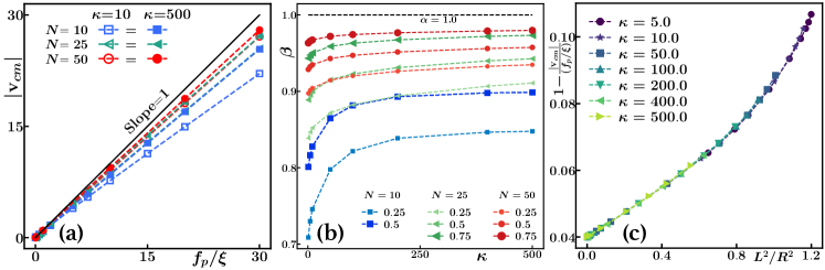
Figure 4: Feedback of curvature on velocity for $\alpha<1$. (a) $|v_{cm}|$ as a function of $f_{p}$ for $\alpha=0.5$, two stiffness values, $\kappa=10$ (open symbols), $\kappa=500$ (filled symbols), and for $N=10$ (blue squares), $N=25$ (green triangles), $N=50$ (red circles). The solid black line of unit slope corresponds to the rigid limit $|v_{cm}|=\frac{f_{p}}{\xi}$. Slopes $\neq 0$ define the velocity reduction factor $\beta$. (b) $\beta$ vs. filament stiffness $\kappa$, for different lengths ($N=10$ $(\blacksquare)$, $N=25~{}(\bullet)$, $N=50~{}(\blacktriangledown)$) and different end-tailoring parameters $\alpha$ (see legend). (c) Approximate scaling for the velocity reduction factor $\beta$, see text.

In the following we mainly focus on the noise-less limit to carve out the features of the end-induced curvature effects. We first study the case when $\alpha<1$, i.e. when the end beads experience a smaller propulsion force than the polymer’s backbone. As for the case $\alpha=1$, there is propulsion in the direction perpendicular to the backbone, but in addition the distribution of the active forces produces a curving along the propulsion direction, as shown in Fig. 1b: since the end beads move more slowly, they lag behind the backbone, and the fiber starts to bend (see also Suppl. movie 1). The conformation of the polymer transiently evolves with time and rapidly attains a stable bent conformation from the balance of the active and the elastic forces, while still propelling transversely with constant velocity.

For not too long polymers ($N\lesssim 25$) the steady conformation is close to a circular arc. We extracted the radius of curvature, $R$, by fitting a circle to the polymer contour. Fig. 3(a) shows the radius of curvature as a function of the propulsion strength rescaled by the filament bending stiffness, $f_{p}/\kappa$, for two different values of $\alpha$, 0.75 and 0.5. As the propulsion force increases, the radius of curvature $R$ decreases (the curvature $C=1/R$ of the polymer increases), until a saturation value is attained that depends on the end-tailoring parameter $\alpha$ – the smaller $\alpha$ and hence the larger the end effect, the smaller the final radius (the higher the curvature). For intermediate driving, there is a scaling regime where $R\propto\left(\frac{f_{p}}{\kappa}\right)^{-1}$, which is expected from slender rod bending theory Landau and Lifschitz (1963). For very small driving, there seems to be another regime where $R\propto\left(\frac{f_{p}}{\kappa}\right)^{-1/2}$, but it will not be observable in the presence of, even small, noise as shown in Fig. 3(b) for $k_{B}T=0.01$. In the presence of noise, the fluctuations (here assumed to be thermal) induce an average bending that can be estimated by equaling thermal energy and bending energy, $k_{B}T\sim\frac{\kappa}{2}\frac{L}{R^{2}}$. From there the system directly crosses over into to $R\propto\left(\frac{f_{p}}{\kappa}\right)^{-1}$ regime.

Fig. 3(c) shows the dependence of the saturated curvature for high propulsion ($R_{\infty}$) on the end tailoring parameter $\alpha$. It can be rationalized by kinematics as follows. Consider the fiber to propel along the $y$-axis and let $\theta$ be the angle between a local tangent and the $x$-axis. Considering one of the two ends, the balance of the following forces must hold: the propulsion force $\alpha f_{p}\mathbf{n}(\theta)$, which is along the local normal $\mathbf{n}(\theta)$, the friction force $-\xi{\bf v}_{cm}$ proportional to the c.o.m. velocity of the fiber in $y$-direction, and the tension force along the local tangent $\mathbf{t}(\theta)$.

Eliminating the tension from the $x$-, $y$-components of the force balance and assuming $\xi{\bf v}_{cm}\simeq f_{p}$ for high driving force (for a detailed study on the relation between shape and velocity, see below), one gets $0=-\alpha f_{p}+\xi{\bf v}_{cm}\cos(\theta)\simeq-\alpha f_{p}+f_{p}\cos(\theta)$. For a circular arc the angle at the filament end is given by $\theta=L/2R$ and hence

$$R_{\infty}=\frac{L}{2\arccos(\alpha)}\,.$$ (7)

For $\alpha=1$, the fiber is straight ($R_{\infty}=\infty$); for $\alpha=0$ this implies $\pi R_{\infty}=L$, corresponding to a half-circle. Fig. 3(c) shows a fit to simulations, confirming the behavior $R_{\infty}\propto 1/\arccos(\alpha)$.

We also investigated the effect of polymer length. In Fig. 3(d), we tried a full scaling collapse, plotting $R/L$ over $B=\frac{f_{p}L^{3}}{\kappa}$ for three different lengths ($N=10,25,50$). While the scaling is fulfilled for every length on its own, there are offsets in both the $f_{p}^{-1}$ scaling regime and the plateau values, implying that the bending is not perfectly circular arc-like. In fact, while the end-tailored propulsion force bends the entire contour of shorter filaments, for longer filaments it affects mostly the boundary regions and the fiber is less curved in the center region.

Let us now discuss the interplay of shape and propulsion velocity. Since the fibers curve and the local propulsion force is orthogonal to the local tangent, bent fibers will move more slowly. The end-tailoring parameter $\alpha$, the stiffness, and the length of the polymer then decide upon the c.o.m. velocity of the filament. As seen in Fig. 4(a), the center of mass velocity $|{\bf v}_{cm}|$ is no longer $f_{p}/\xi$, but reduced by a factor $\beta(\alpha,\kappa,N)$. The value of $\beta$ was extracted from the slope of a straight line fit to $|v_{cm}|$ as a function of $f_{p}$, for a given $\kappa$ and $N$. The resulting $\beta$ for different values of $\alpha$ and $N$ are shown in Fig. 4(b) as a function of stiffness $\kappa$. For a given $\alpha$, due to the end-induced deformation propagating to the middle of filament, short and flexible filaments curve more and propel slower than longer filaments that curve less and translate faster for the same value of propulsion strength.

This observed velocity reduction is mostly a kinematic, shape-induced effect, as can be seen as follows. The propulsion force is $f_{p}\mathbf{n}$, except for the ends. Neglecting the details of the end effects, but including their main effect, i.e. the curving of the fiber to an approximately circular arc, the total force in propulsion direction is given by (using symmetry) $F_{tot}=2f_{p}\int_{0}^{L/2}\cos\theta(s)\,ds$. For a circular arc, one has $\theta(s)=\theta_{e}-s/R$ with the end angle $\theta_{e}=\frac{L}{2R}$. Evaluating $F_{tot}$, expanding in $L/(2R)$ and equaling to the total friction force yields for the c.o.m. velocity

$${\mathbf{v}_{cm}}=\frac{f_{p}}{\xi}\left[1-c\left(\frac{L}{R}\right)^{2}\right].$$ (8)

Here $c$ is a constant (in this crude approximation $c=\frac{1}{24}$) and the radius of curvature $R=R(\alpha,\kappa,f_{p})$ is a complicated function of end-tailoring, stiffness and propulsion as investigated in Fig. 3. Note that, if $R$ were not dependent on the propulsion force $f_{p}$, the term in brackets in Eq. (8) would just be $\beta$.

If indeed the velocity reduction is due to the curving via simple kinematics, plotting $1-\frac{\mathbf{v}_{cm}}{f_{p}/\xi}$ over $(L/R)^{2}$ should yield a constant. Fig. 4(c) shows the result: first, there is a small offset, due to the reduced propulsion (due to $\alpha<1$) at the ends. In fact, in the shown case 2 out of 25 beads are propelled with a fraction $\alpha=0.5$ of $f_{p}$ only, which reduces the overall propulsion velocity by $0.04$. For finite $(L/R)^{2}$ there is a quite weak dependence (of the same order as the end effect). Taking into account that the scaling, containing data from several orders of magnitude of both $\kappa$ and $f_{p}$, works well shows that the kinematics of circular arcs gives a rather good description. Note that one can also apply the reasoning suggested by Eq. (8) locally: wherever there is a curvature along the polymer contour, this leads to a reduction of the local velocity. This simple point of view will be useful for more complex polymer morphologies, cf. the next section.

V Faster end beads ($\alpha>1$) and complex dynamics

Finally, we consider the case of $\alpha>1$, where the end beads move faster than the polymer backbone. The distribution of the active propulsion then leads to a curving of the filament in the direction opposite to propulsion, see Fig 1b and Suppl. movie 2. As can be seen there, for weak end-tailoring $\alpha>1$, the shape is just a mirror image of the case $\alpha<1$. However, for stronger $\alpha>1$, the behaviour becomes much more complex than for the case just described, with strong deviations from the circular arc shape and even an instability to oscillatory, flapping-like dynamics.

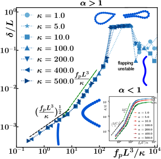
Figure 5: Shape deformations for $\alpha>1$. The scaled maximum amplitude of deformation $(\delta/L)$ is shown as a function of $B=f_{p}L^{3}/\kappa$ for $\alpha=1.5$. Except for the dynamic states at high $B$, the data for different stiffnesses collapse. Selected polymer conformations in the different regimes are presented. For comparison, the inset displays data for the case $\alpha<1$.

To characterise these bent shapes, instead of the radius of curvature, we hence opted for the bending amplitude $\delta$, defined as the distance to the maximum curved point on the polymer contour (${\bf r}_{Cmax}$) from the center of mass of the end beads (${\bf r}_{cm}^{1,N}$),

$$\delta=|{\bf r}_{Cmax}-{\bf r}_{cm}^{1,N}|.$$ (9)

Fig 5 traces the scaled version $\delta/L$ as a function of $B=f_{p}L^{3}/\kappa$ together with corresponding typical steady-state conformations. For comparison, the same plot for the case $\alpha<1$ is given in the inset.

One can see from Fig 5 that the scaling regimes, corresponding to those observed in the radius of curvature in Fig. 3, are again visible. However, in the case $\alpha>1$ there is not just saturation of curving (as for $\alpha<1$, cf. the inset), but complex shapes and even dynamic behavior can emerge:

At $B\gtrsim 250$ for the given $\alpha=1.5$, a sudden jump in $\delta$ occurs. This transition can be ascribed to the emergence of 2Dloop or hairpin structures, which form when the end beads of the polymer come into contact with each other, cf. the snapshots in Fig 5 and Suppl. movie 3 and 4, respectively. Once they fold on to each other, the self-avoiding interaction comes into play, but the larger propulsion force of the ends keeps the structure together. Typically, one end bead sits at the void between two beads of the opposite end, forming a bead-triplet configuration. Either a drop-shaped 2Dloop or a hairpin conformation is formed, where in the latter several beads close to the ends form a quasi 1D triangular lattice-like arrangement, see the snapshots in Fig. 5. While establishing the final shape, the polymer is almost stationary. The final polymer conformation, however, exhibits a stable rotational motion, since opposing beads cancel their propulsion, but only partially for reasons of shape asymmetry. Hence the center of mass of both the $2Dloop$ and $hairpin$ conformation then follow a circular path, the period of rotation being mostly determined by $f_{p}$.

At even higher drive, $B\gtrsim 1600$ for the given $\alpha=1.5$, an instability occurs, visible in Fig. 5 by a drop of $\delta$. Here an initially straight polymer forms a W-shaped conformation that is highly dynamic, with the ends flapping in an oscillatory fashion. A time-lapse of the conformational changes of such a cycle is shown in Fig. 6(a). As can be seen the ends, being faster, “roll up”. In doing so, however, they contribute less to propulsion, hence the initially rather straight middle catches up and starts to bulge out. This curving, however, slows the middle down, cf. Eq. (8) and the concomitant elastic deformation leads to an unfolding of the ends and finally the polymer attains its initial W-shape again, see also Suppl. movie 5.

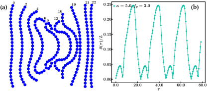
Figure 6: Flapping motion for $\alpha>1$ and large $B$ values. (a) A series of conformations is shown during one period (the resulting period is $23\tau$) of the flapping instability. The fiber propells to the right. Parameters: $\alpha=1.5$ and $B\simeq 5530$ ($\kappa=5$, $f_{p}=2$, $L=25$). (b) Several oscillation periods are shown for the scaled maximum amplitude of deformation, $\delta/L$, corresponding to the shapes shown in (a).

Note that in Fig. 5, we always started from a straight initial conformation to which the propulsion force was added. We also investigated whether transitions between the different types of conformations are possible when changing the parameters $\alpha$ and/or $f_{p}$ for already established conformations. Transitions between 2Dloop and hairpin are possible, but if a fiber had already a closed 2Dloop or hairpin shape it was not possible to directly induce the flapping W-shape by small continuous parameter changes, i.e. this state seems to be accessible only from initially roughly straight conformations.

From the bent shapes observed in Fig. 5 one would again expect a reduction in velocity compared to straight fibers. For small deviations from $\alpha=1$, the system is mirror symmetric, cf. the snapshots in Fig. 1, and the velocity reduction for $\alpha>1$ is as for $\alpha<1$, i.e. roughly given by Eq. (8), albeit with an offset of opposite sign due to the stronger propulsion of the end beads. For the more complex shapes, 2Dloop, hairpin and W-shape, the velocity is even further reduced, since more beads are pointing in directions not contributing to propulsion or due to the oscillatory dynamics, respectively.

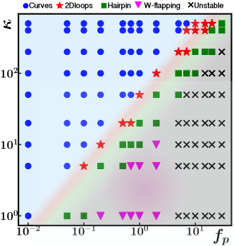
Figure 7: State diagram in the $\kappa{-}f_{p}$ plane for $\alpha=1.5$, $N=25$. The different conformations were identified by their values of $\delta/L$, end-to-end distance $R_{E}$ and by visually checking. Crossovers between states are indicated by shading and serve as a guide to the eye.

Finally Fig. 7 displays a state diagram of the different conformations attained by an initially straight polymer with $\alpha=1.5$ and $N=25$, in the plane stiffness $\kappa$ vs. propulsion force $f_{p}$. For different lengths, such $\kappa{-}f_{p}$ diagrams look qualitatively the same, but overall there is no good data collapse using scaling, for the same reason as in the discussion of Fig. 3. Also, for very short filaments ($N=5$), having too few degrees of freedom, the complex conformations like the flapping are completely absent. Nevertheless, as can be seen in Fig 7, as the stiffness increases the simple curved conformations dominate and the $2Dloop/hairpin$ conformations are shifted to higher values of $f_{p}$. The flapping mode occurs at low values of $\kappa$ and moderate value of $f_{p}$. Very large driving forces $f_{p}$ promote asymmetric polymer conformations that are erratic/chaotic in time, denoted in the diagram as “unstable” and indicating that the system cannot adopt anymore simple, stable or time-periodic, states.

VI Summary and outlook

In this work, we used Langevin dynamics simulations to study the conformational properties of an active semi-flexible polymer that experiences local propulsion forces in the direction perpendicular to its contour. In addition the polymer is end-tailored, i.e. the end beads have slightly different propulsion properties. We considered self-avoiding interactions but for simplicity assumed the dry limit, i.e. solvent-mediated hydrodynamic interactions are ignored and friction is isotropic.

We have shown that the conformational properties can be tuned by the relative propulsion strength between the end beads and the polymer backbone and that a rich state diagram emerges from the interaction of propulsion and flexibility. If the ends beads move slower than the backbone (end-tailoring parameter $\alpha<1$), the polymer deforms to a bent conformation, and the curvature of the polymer is along the propulsion direction. The radius of curvature/the deformation amplitude shows scaling regimes due to the interplay of bending and active forces and a saturation regime at high propulsion where further increasing the propulsion force only stretches the polymer. Dynamic shapes as for $\alpha<1$ share similarities with bent conformations observed for moving filaments under a uniform field Lagomarsino et al. (2005); Marchetti et al. (2019) and with shapes of rolling fibers driven by an energy flow through their cross-section leading to a differential contraction Bazir et al. (2020).

When the end beads move faster than the backbone ($\alpha>1$), we have shown that different dynamic conformations emerge as a function of stiffness and propulsion strength. For small propulsion a bent conformation with a curvature opposite to the propulsion direction is obtained. For intermediate propulsion strength, the polymer can close into a rotating 2Dloop or hairpin conformation. Finally, for even larger driving the interplay between activity and flexibility can trigger a dynamic state of the polymer, which propells sideways while flapping around a W-shape conformation. Bent shapes as for $\alpha>1$ have been observed for rolling fibers driven by an energy flow through their cross-section leading to differential expansion Bazir et al. (2020). Dynamic W-shapes were previously observed for sedimenting filaments in a viscous fluid Lagomarsino et al. (2005). Nevertheless, here the situation is different, because the propulsion is in the transverse direction locally along the fiber shape, unlike for sedimentation.

We studied here only a single active polymer. In the last few years various collective effects have been extensively studied for ensembles of tangentially propelled objects Peruani et al. (2012); Schaller et al. (2010); Marchetti et al. (2013); Prathyusha et al. (2018); Duman et al. (2018). In the context of their pattern formation and collective behaviour, however, transversely propelled objects should belong to a different symmetry class as the tangential ones. As more and more such transverse propellers are being designed Tierno et al. (2010); Vutukuri et al. (2016); Rao et al. (2019); Doherty et al. (2020) it will be interesting to investigate their possibly different collective effects in the future. Note that again flexibility will be important: namely, transversely propelled rigid colloidal janus rods were shown to rather block each other leading to clustering and arrest of motion Vutukuri et al. (2016). In contrast, self-rolling flexible fibers were shown to be able to switch direction by defoming under collisions Bazir et al. (2020), which allows for more interesting collective behavior.

On the application side, sideways propellers have been already suggested to catch particles Arslanova et al. (2021). Especially, catalase-powered enzymatic Janus micromotors were already demonstrated to be able to capture bacteria Zhao et al. (2019) and tumor cells Zhao et al. (2020). As we demonstrated here, including flexibility and adding “end-tailoring” substantially increases the possible conformations achievable for sideways propelled objects which in addition are dynamic, i.e. switchable via the fuel, hence opening up new routes for the design of self-driven microrobotic engines.

References

- Gompper et al. (2020) G. Gompper, R. G. Winkler, T. Speck, A. Solon, C. Nardini, F. Peruani, H. Löwen, R. Golestanian, U. B. Kaupp, L. Alvarez, T. Kiørboe, E. Lauga, W. C. K. Poon, A. DeSimone, S. Muiños-Landin, A. Fischer, N. A. Söker, F. Cichos, R. Kapral, P. Gaspard, M. Ripoll, F. Sagues, A. Doostmohammadi, J. M. Yeomans, I. S. Aranson, C. Bechinger, H. Stark, C. K. Hemelrijk, F. J. Nedelec, T. Sarkar, T. Aryaksama, M. Lacroix, G. Duclos, V. Yashunsky, P. Silberzan, M. Arroyo, and S. Kale, J. Phys.: Condens. Matter 32, 193001 (2020).
- Berg and Anderson (1973) H. C. Berg and R. A. Anderson, Nature 245, 380 (1973).
- Lauga and Powers (2009) E. Lauga and T. R. Powers, Rep. Prog. Phys. 72, 096601 (2009).
- Mauriello et al. (2010) E. M. F. Mauriello, T. Mignot, Z. Yang, and D. R. Zusman, Microbiol. Mol. Biol. Rev. 74, 229 (2010).
- Peruani et al. (2012) F. Peruani, J. Starruß, V. Jakovljevic, L. Sogaard-Andersen, A. Deutsch, and M. Bär, Phys. Rev. Lett. 108, 098102 (2012).
- Ray et al. (1993) S. Ray, E. Meyhöfer, R. A. Milligan, and J. Howard, J. Cell Biol. 121, 1083 (1993).
- Schaller et al. (2010) V. Schaller, C. Weber, C. Semmrich, E. Frey, and A. R. Bausch, Nature 467, 73 (2010).
- Paxton et al. (2004) W. F. Paxton, K. C. Kistler, C. C. Olmeda, A. Sen, S. K. S. Angelo, Y. Cao, T. E. Mallouk, P. E. Lammert, and V. H. Crespi, J. Am. Chem. Soc. 126, 13431 (2004).
- Ebbens et al. (2012) S. Ebbens, M.-H. Tu, J. R. Howse, and R. Golestanian, Phys. Rev. E 85, 020401(R) (2012).
- Howse et al. (2007) J. R. Howse, R. A. L. Jones, A. J. Ryan, T. Gough, R. Vafabakhsh, and R. Golestanian, Phys. Rev. Lett. 99, 048102 (2007).
- Soto and Golestanian (2014) R. Soto and R. Golestanian, Phys. Rev. Lett. 112, 068301 (2014).
- Buttinoni et al. (2012) I. Buttinoni, G. Volpe, F. Kümmel, G. Volpe, and C. Bechinger, J. Phys. Cond. Matt. 24, 284129 (2012).
- Tierno et al. (2010) P. Tierno, R. Albalat, and F. Sagues, Small 16, 1749 (2010).
- Vutukuri et al. (2016) H. R. Vutukuri, Z. Preisler, T. H. Besseling, A. van Blaaderen, M. Dijkstra, and W. T. S. Huck, Soft Matter 12, 9657 (2016).
- Rao et al. (2019) D. V. Rao, N. Reddy, J. Fransaer, and C. Clasen, J. Phys. D. Apply. Phys. 52, 014002 (2019).
- Doherty et al. (2020) R. P. Doherty, T. Varkevisser, M. Teunisse, J. Hoecht, S. Ketzetzi, S. Ouhajji, and D. J. Kraft, Soft Matter 16, 10463 (2020).
- Vutukuri et al. (2017) H. R. Vutukuri, B. Bet, R. van Roij, M. Dijkstra, and W. T. S. Huck, Sci. Rep 7, 16758 (2017).
- Baumann et al. (2018) A. Baumann, A. Sanchez-Ferrer, L. Jacomine, P. Martinoty, V. L. Houerou, F. Ziebert, and I. M. Kulic, Nat. mater. 17, 523 (2018).
- Bazir et al. (2020) A. Bazir, A. Baumann, F. Ziebert, and I. M. Kulic, Soft Matter 16, 5210 (2020).
- Jiang et al. (2021) Z.-C. Jiang, Y.-Y. Xiao, R.-D. Cheng, J.-B. Hou, and Y. Zhao, Chem. Mater. 33, 6541 (2021).
- Yan et al. (2016) J. Yan, M. Han, J. Zhang, C. Xu, E. Luijten, and S. Granick, Nat. Mater. 15, 1095 (2016).
- Jayaraman et al. (2012) G. Jayaraman, S. Ramachandran, S. Ghose, A. Laskar, M. S. Bhamla, P. B. S. Kumar, and R. Adhikari, Phys. Rev. Lett. 109, 158302 (2012).
- Isele-Holder et al. (2015) R. E. Isele-Holder, J. Elgeti, and G. Gompper, Soft Matter 11, 7181 (2015).
- Eisenstecken et al. (2016) T. Eisenstecken, G. Gompper, and R. G. Winkler, Polymers 8, 304 (2016).
- Jiang and Hou (2014) H. Jiang and Z. Hou, Soft Matter 10, 1012 (2014).
- Lagomarsino et al. (2005) M. C. Lagomarsino, I. Pagonabarraga, and C. P. Lowe, Phys. Rev. Lett. 94, 148104 (2005).
- Xu and Nadim (1994) X. Xu and A. Nadim, Phys. Fluids 9, 2890 (1994).
- Schlagberger and Netz (2005) X. Schlagberger and R. R. Netz, Euro. Phys. Lett. 70, 129 (2005).
- Marchetti et al. (2019) B. Marchetti, V. Raspa, A. Lindner, O. du Roure, L. Bergougnoux, É. Guazzelli, and C. Duprat, Phys. Rev. Fluids 3, 104102 (2019).
- Weeks et al. (1971) J. D. Weeks, D. Chandler, and H. C. Andersen, J. Chem. Phys. 54, 5237 (1971).
- Kremer and Grest (1990) K. Kremer and G. S. Grest, J. Chem. Phys. 92, 5057 (1990).
- Plimpton (1995) S. Plimpton, J. Chem. Phys. 117, 1 (1995).
- Golestanian (2009) R. Golestanian, Phys. Rev. Lett. 102, 188305 (2009).
- Schol et al. (2018) C. Schol, S. Jahanshahi, A. Ldov, and H. Löwen, Nat. Comm. 9, 5156 (2018).
- Doi and Edwards (1986) M. Doi and S. F. Edwards, The theory of polymer dynamics (Oxford University Press, Newyork, 1986).
- Landau and Lifschitz (1963) L. D. Landau and E. M. Lifschitz, The theory of elasticity 2nd Edition (Pergamon Press, Oxford, Newyork, 1963).
- Marchetti et al. (2013) M. Marchetti, J. Joanny, S. Ramaswamy, T. Liverpool, J. Prost, M. Rao, and R. A. Simha, Rev. Mod. Phys. 85, 1143 (2013).
- Prathyusha et al. (2018) K. R. Prathyusha, S. Henkes, and R. Sknepnek, Phys. Rev. E 97, 022606 (2018).
- Duman et al. (2018) Ö. Duman, R. E. Isele-Holder, J. Elgeti, and G. Gompper, Soft Matter 14, 4483 (2018).
- Arslanova et al. (2021) A. Arslanova, V. R. Dugyala, E. K. Reichel, N. Reddy, J. Fransaer, and C. Clasen, Soft Matter 17, 2369 (2021).
- Zhao et al. (2019) L. Zhao, S. Xie, Y. Liu, Q. Liu, X. Song, and X. Li, Nanoscale 11, 17831 (2019).
- Zhao et al. (2020) L. Zhao, Y. Liu, S. Xie, P. Ran, J. Wei, Q. Liu, and X. Li, Chem. Eng. J. 382, 123041 (2020).