Final results on the $0\nu\beta\beta$ decay half-life limit of ¹⁰⁰Mo from the CUPID-Mo experiment

Abstract

The CUPID-Mo experiment to search for 0$\nu\beta\beta$ decay in ¹⁰⁰Mo has been recently completed after about 1.5 years of operation at Laboratoire Souterrain de Modane (France). It served as a demonstrator for CUPID, a next generation 0$\nu\beta\beta$ decay experiment. CUPID-Mo was comprised of 20 enriched Li₂¹⁰⁰MoO₄ scintillating calorimeters, each with a mass of $\sim$ 0.2  kg, operated at $\sim$20  mK. We present here the final analysis with the full exposure of CUPID-Mo (¹⁰⁰Mo exposure of 1.47 kg$\times$year) used to search for lepton number violation via 0$\nu\beta\beta$ decay. We report on various analysis improvements since the previous result on a subset of data, reprocessing all data with these new techniques. We observe zero events in the region of interest and set a new limit on the ¹⁰⁰Mo 0$\nu\beta\beta$ decay half-life of $T_{1/2}^{0\nu}$ $>{\color[rgb]{0,0,0}{1.8}}\times 10^{24}$ year (stat.+syst.)  at 90% CI. Under the light Majorana neutrino exchange mechanism this corresponds to an effective Majorana neutrino mass of $\left<m_{\beta\beta}\right>$ $<$ $(0.28$–$0.49)$  eV, dependent upon the nuclear matrix element utilized.

1 Introduction

Ever since the neutrino was found to have mass via the observation of flavor state oscillations PhysRevLett.81.1562 ; Ahmad2001 , the nature of the neutrino mass itself has remained a mystery. Unlike charged leptons, neutrinos may be Majorana MajoranaPaper ; PhysRevD.22.2227 instead of Dirac particles. In addition to implying that neutrinos and anti-neutrinos would be the same particle Racah1938 , this would also imply that the total lepton number is not conserved Pontecorvo1968 . This may provide for a possible explanation of baryon asymmetry (i.e., the imbalance between matter and anti-matter) in the early universe FUKUGITA198645 ; DAVIDSON2008105 .

Two-neutrino double-beta (2$\nu\beta\beta$) decay is a rare Standard Model process which can occur in some even-even nuclei for which single beta decays are energetically forbidden (or heavily disfavored due to large changes in angular momentum). In this process two neutrons are converted into two protons with the emission of two electrons and two electron anti-neutrinos. The possibility of the neutrino being a Majorana fermion raises the prospect that neutrinoless double-beta (0$\nu\beta\beta$) decay may occur Furry1939 ; PhysRevD.25.2951 . In the case of 0$\nu\beta\beta$ decay, we would again observe the conversion of two neutrons into two protons, but such a decay would only produce two electrons. Whereas 2$\nu\beta\beta$ decay conserves lepton number, 0$\nu\beta\beta$ decay would result in an overall violation of the total lepton number by two units Bilenky2015 ; Goswami2015 ; Dolinski2019 , and indicate physics beyond the Standard Model. At present this process is unobserved with limits on the decay half-life at the level of $10^{24}-10^{26}$  year via the isotopes ⁷⁶Ge, ⁸²Se, ¹⁰⁰Mo, ¹³⁰Te, and ¹³⁶Xe GERDA2020 ; MJD2019 ; CUPID0Final ; CUORE1ton ; CUOREPRL2020 ; CuMoPRL ; NEMO30vMo ; KamLANDZen2016 ; EXO200.2019 . The process of 0$\nu\beta\beta$ decay has several possible mechanisms Bilenky2015 ; Dolinski2019 ; Deppisch2012 ; Rodejohann2012 ; PhysRevD.68.034016 ; Atre2009 ; Blennow2010 ; MITRA201226 ; Cirigliano2018 , however the minimal extension to the Standard Model provides the simplest via the exchange of a light Majorana neutrino. The rate of this process is dependent upon the square of the effective Majorana neutrino mass, $\left<m_{\beta\beta}\right>$:

$$\Gamma^{0\nu}=G^{0\nu}g^{4}_{A}|M^{0\nu}_{\beta\beta}|^{2}|\langle m_{\beta\beta}\rangle|^{2}/m_{e}^{2},$$ (1)

where $g_{A}$ is the weak axial vector coupling constant, $M^{0\nu}_{\beta\beta}$ is the nuclear matrix element, $G_{0\nu}$ is the decay phase space, and $m_{e}$ is the electron mass. The effective mass is a linear combination of the three neutrino mass eigenstates, with the present limits on $\left<m_{\beta\beta}\right>$ ranging from 60–600  meV Dolinski2019 .

A vibrant experimental field has emerged to search for 0$\nu\beta\beta$ decay with experiments using a variety of nuclei and a wide range of methods (see Dolinski2019 for a review of some of these). The main experimental signature for this decay is a peak of the summed electron energy at the $Q$-value of the decay ($Q_{\beta\beta}$; the difference in energy between the parent and daughter nuclei) broadened only by detector energy resolution. There are 35 natural $\beta\beta$ decay isotopes TRETYAK200283 , however from an experimental perspective only a subset of these are relevant. Searching for 0$\nu\beta\beta$ decay requires that the number of target atoms should be very large and that the background rate should be small. In an ideal case a candidate isotope should have $Q_{\beta\beta}$ ¿ 2.6  MeV so it is above significant natural $\gamma$ backgrounds and has the phase space for a relatively fast decay rate. It should also occur with a high natural abundance or be easily enriched.

The isotope ¹⁰⁰Mo meets these requirements with a $Q_{\beta\beta}$ of 3034  keV and a relatively favorable phase space compared to other isotopes. Additionally it is relatively easy to enrich detectors with ¹⁰⁰Mo. Several experiments have utilized ¹⁰⁰Mo for 0$\nu\beta\beta$ decay searches: NEMO-3, LUMINEU, and AMoRE. NEMO-3 utilized foils containing ¹⁰⁰Mo and used external sensors to measure time of flight and provide calorimetry. It ran from 2003-2010 at Modane and accumulated an exposure of 34.3 kg$\times$year in ¹⁰⁰Mo. It found no evidence for 0$\nu\beta\beta$ and set a limit of $T_{1/2}^{0\nu}$ $>1.1\times 10^{24}$ year  at 90% C.I. with a limit on the effective Majorana mass of $\left<m_{\beta\beta}\right>$ $<$ $(0.33$–$0.62)$  eV NEMO30vMo . LUMINEU was a pilot experiment for ¹⁰⁰Mo based calorimeters and served as a precursor to CUPID-Mo. LUMINEU utilized both Zn¹⁰⁰MoO₄ and Li₂¹⁰⁰MoO₄ crystals, and found Li₂¹⁰⁰MoO₄ is more favorable for 0$\nu\beta\beta$ decay searches lumineu2017 . AMoRE operates at Yangyang underground laboratory in Korea. The AMoRE-pilot operated with ${}^{48\text{depl}}$Ca¹⁰⁰MoO₄ crystals. As with CUPID-Mo, AMoRE utilizes light and heat to provide particle identification. The AMoRE-pilot has set a limit using 111 kg$\times$day of exposure of $T_{1/2}^{0\nu}$ $>9.5\times 10^{22}$ year  at 90% C.I. with a corresponding effective Majorana mass limit of $\left<m_{\beta\beta}\right>$ $<$ $(1.2$–$2.1)$  eV AMORE2019 .

Scintillating calorimeters are one of the most promising current technologies for 0$\nu\beta\beta$ decay searches, with many possible configurations DPoda2021 ; PirroScintBolo ; Tabarelli2009 ; Cardani2013LMO ; Giuliani2018 ; CUPID0Final ; AMORE2019 ; sym13122255 . These consist of a crystalline material, containing the source isotope, capable of scintillating at low temperatures which is operated as a cryogenic calorimeter coupled to light detectors to detect scintillation light. Particle identification is based on the difference in scintillation light produced for a given amount of energy deposited in the main calorimeter. This technology has demonstrated excellent energy resolution, high detection efficiency, and low background rates (due to the rejection of $\alpha$ events). The rejection of $\alpha$ events is of primary concern as the energy region above $\sim$2.6  MeV is populated by surface radioactive contaminants with degraded energy collection of $\alpha$ particles CUORE1ton ; CUOREPRL2020 .

CUPID (CUORE Upgrade with Particle IDentification) is a next-generation experiment CUPID:2019 which will use this scintillation calorimeter technology. It will build on the success of CUORE (Cryogenic Underground Observatory for Rare Events) which demonstrated the feasibility of a tonne-scale experiment using cryogenic calorimeters CUORE_cryostat ; CUORE1ton . In this paper we describe the final 0$\nu\beta\beta$ decay search results of the CUPID-Mo experiment which has successfully demonstrated the use of ¹⁰⁰Mo-enriched Li₂MoO₄ detectors for CUPID. In sections 2 and 3 we introduce the CUPID-Mo experiment and an overview of the collected data. In sections 4 and 5 we describe the data production and basic data quality selection. Then in sections 6–11 we describe in detail the improved data selection cuts we use to reduce experimental background rates. We then describe our Bayesian 0$\nu\beta\beta$ decay analysis in sections 12–14. Finally, the results and their implications are discussed in section 15.

2 CUPID-Mo Experiment

The CUPID-Mo experiment was operated underground at the Laboratoire Souterrain de Modane in France CuMo_instrument following a successful pilot experiment, LUMINEU lumineu2017 ; Poda2017 . The CUPID-Mo detector array was comprised of 20 scintillating Li₂MoO₄ (LMO) cylindrical crystals, $\sim$210  g each (see Fig. 1). These are enriched in ¹⁰⁰Mo to $\sim$97%, and operated as cryogenic calorimeters at $\sim 20$  mK. Each LMO detector is paired with a Ge wafer light detector (LD) and assembled into a detector module with a copper holder and Vikuiti${}^{\text{TM}}$ reflective foil to increase scintillation light collection. Both the LMO detectors and LDs are instrumented with a neutron-transmutation doped Ge-thermistor (NTD) Haller1984 for data readout. Additionally, a Si heater is attached to each LMO crystal which is used to monitor detector performance.

The modules are organized into five towers with four floors and mounted in the EDELWEISS cryostat Armengaud_2017 (see Fig. 1). In this configuration each LMO detector (apart from those on the top floor) nominally has two LDs increasing the discrimination power. We note that one LD did not function resulting in two LMO detectors which are not on the top floor having only a single working LD.

CUPID-Mo has demonstrated excellent performance, crystal radiopurity, energy resolution, and high detection efficiency CuMo_instrument , close to the requirements of the CUPID experiment CUPID:2019 . An analysis of the initial CUPID-Mo data (1.17 kg$\times$year of ¹⁰⁰Mo exposure) led to a limit on the half-life of 0$\nu\beta\beta$ decay in ¹⁰⁰Mo of $T_{1/2}^{0\nu}>1.5\times 10^{24}$yr  at 90% C.I. CuMoPRL . For the final results of CUPID-Mo we increase the exposure and also develop novel analysis procedures which will be critical to allow CUPID to reach its goals.

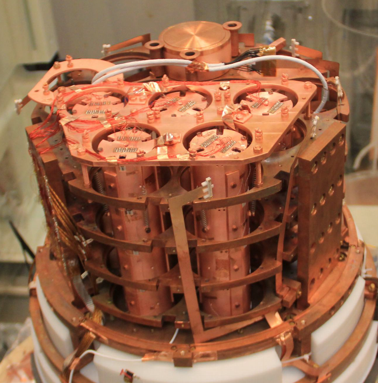
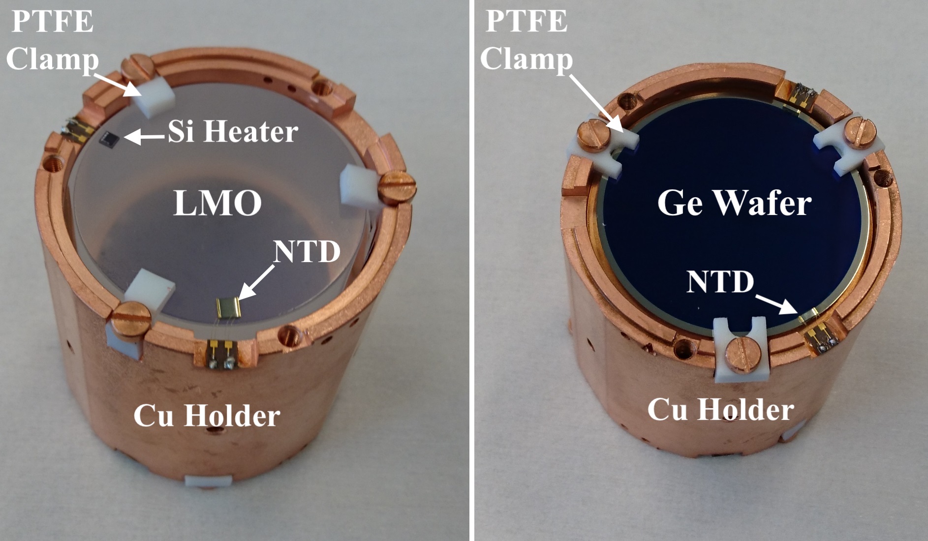
Figure 1: Images showing the CUPID-Mo detector array (5 nearest towers) mounted in the EDELWEISS cryostat (Top) and a single module assembled in the Cu holder (Bottom) CuMo_instrument . (Bottom left) view from the top on the LMO detector, NTD-Ge, Si heater, copper holder and PTFE clamps. (Bottom right) view from the bottom on the Ge LD and its NTD-Ge thermistor and PTFE clamps.

3 CUPID-Mo Data Taking

The data utilized in this analysis was acquired from early 2019 through mid-2020 (481 days in total) with a duty cycle of $\sim$89% of the EDELWEISS cryogenic facility. The data collected between periods of cryostat maintenance or special calibrations, which require the external shield to open, are grouped into “datasets” typically $\sim$1–2 months long. Within each dataset we attempt to have periods of calibration data taking (typically, $\sim$2-d-long measurements every $\sim$10 days) bracketing physics data taking, corresponding to 21% and 70% of the total CUPID-Mo data respectively. CUPID-Mo utilizes a U/Th source placed outside the copper screens of the cryostat (see CuMo_instrument ) for standard LMO detector calibration, providing a prominent $\gamma$ peak at 2615  keV, as well as several other peaks at lower energies to perform calibration. The primary calibration source is a thorite mineral with $\sim$50 Bq of ²³²Th, and $\sim$100 Bq of ²³⁸U with significantly smaller activity from ²³⁵U. Overall, nine datasets are utilized in this final analysis with a total LMO exposure of 2.71  kg$\times$year, corresponding to a ¹⁰⁰Mo exposure of 1.47  kg$\times$year. As was the case in the previous analysis CuMoPRL , we exclude three short periods of data taking which have an insufficient amount of calibration data to adequately perform thermal gain correction, and determine the energy calibration. We also exclude one LMO detector which has abnormally poor performance in all datasets.

Additional periods of data taking with a very high activity ⁶⁰Co source ($\sim$100 kBq, $\sim$2% of CUPID-Mo data) were performed near regular liquid He refills (every $\sim$ 10 days). While the ${}^{60}\mathrm{Co}$ source was primarily used for EDELWEISS Armengaud_2017 , it was also utilized in CUPID-Mo for LD calibration via X-ray fluorescence CuMo_instrument and is further described in section 4.3. The remainder of the data in CUPID-Mo is split between calibration with a ²⁴¹Am+⁹Be neutron source (2%) and a ⁵⁶Co calibration source ($\sim$5%).

4 Data Production

We outline here the basic data production steps required to create a calibrated energy spectrum. Starting with AC biased NTDs, we perform demodulation in hardware and sample the resulting voltage signals from all heat and light channels at 500  Hz to produce the raw data. We then utilize the Diana and Apollo framework PhysRevC.93.045503 ; Apollo_Domizio_2018 , developed by the CUORE-0, CUORE, and CUPID-0 collaborations, with modifications for CUPID-Mo. Events in data are triggered “offline” in Apollo using the optimum trigger method OT_Domizio_2011 to search for pulses. This method requires an initial triggering of the data to construct an average pulse template and average noise power spectrum. This in turn is used to build an optimum filter (OF) which maximizes the signal-to-noise ratio. This OF is then used as the basis for the primary triggering. An event is triggered when the filtered data crosses a set threshold relative to the typical OF resolution obtained from the average noise power spectrum for a given channel (set at a value of 10$\sigma$). We periodically inject flags to indicate noise triggers into the data stream in order to obtain a sample of noise events which allows us to characterize the noise on each channel. For this data production we utilize a 3 s time window for both the heat and light channels. This is long enough to allow sufficient time for the LMO waveform to return towards baseline whilst being short enough to keep the rate of pileup events relatively low. This choice also keeps the event windows of equal size between the LMO detectors and LDs (see Fig. 2). The first 1 s of data prior to the trigger is the pretrigger window which is used in pulse baseline measurements. For reference the typical 10%–90% rise and 90%–30% fall times for the LMO detectors are $\sim$20  ms and $\sim$300  ms respectively, and for the LDs they are much shorter at $\sim$4  ms and $\sim$9  ms respectively CuMo_instrument .

Once triggered data is available, basic event reconstruction quantities are computed, such as the waveform average baseline (the mean of the waveform in the first 80% of the pretrigger window), baseline slope, pulse rise and decay times, and other parameters that are computed directly on the raw waveform. A mapping of so-called “side” channels is generated, grouping the LDs that a given LMO crystal directly faces in the data processing framework. In each dataset, a new OF is constructed for each channel, and used to estimate the amplitude of both the LMO detector and LD events, the latter being restricted to search in a narrow range around the LMO event trigger time. After the OF amplitudes are available, thermal gain correction is performed on the LMO detectors (see section 4.1) and finally the LMO detector energy scale is calibrated from the external U/Th calibration runs (see section 4.2). Each step of the data production is done on runs within a single dataset, with the exception of the first two datasets which share a common thermal gain correction and energy calibration period to boost statistics.

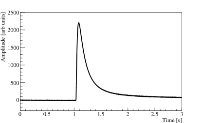
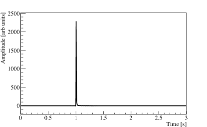
Figure 2: Typical average pulses for LMO detector (top) and LD (bottom) readout. Note that the LMO pulses are significantly longer in duration owing to the larger heat capacity of the LMO compared to the much smaller Ge LD.

4.1 Thermal Gain Correction

After we have reconstructed pulse amplitudes via the OF we must perform a thermal gain correction (sometimes referred to as “stabilization”) Alessandrello1998 . This process corrects for thermal-gain changes in detector response which cause slight differences in pulse amplitude for a given incident energy, resulting in artificially broadened peaks. The pulse baseline is used as a proxy for the temperature, allowing us to use it to correct for thermal-gain changes due to fluctuations in temperature. This correction uses calibration data, from which we select a sample of events determined to be the 2615  keV $\gamma$-ray full absorption peak from ²⁰⁸Tl. We perform a fit of the OF amplitudes ($A$) as a function of the mean baselines ($b_{\mu}$) given by the linear function $f(b_{\mu})=p_{0}+p_{1}\cdot b_{\mu}$ and compute the scaled corrected amplitude ($\tilde{C}$) as $\tilde{C}=(A/f(b_{\mu}))\cdot 2615$. This correction is applied to both calibration and physics data within a dataset. We observe that the LDs do not demonstrate any significant thermal gain drift and as such do not perform this step on them.

4.2 LMO Detector Calibration

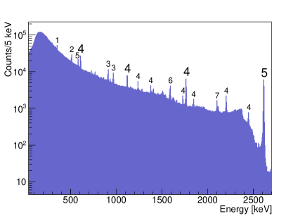
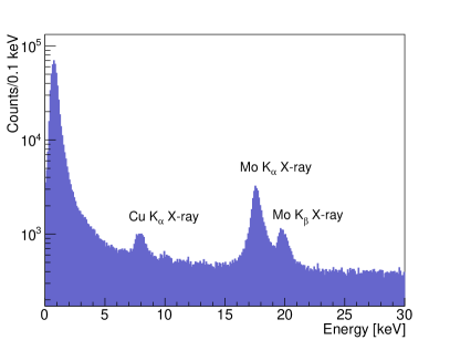
Figure 3: CUPID-Mo calibration spectra for both LMO detectors and LDs. Left: Calibration spectra for LMO detectors exposed to the ²³²Th/²³⁸U source. A selection of the most prominent peaks are labeled: (1) ²¹⁴Pb, (2) $e^{-}e^{+}$ annihilation, (3) ²²⁸Ac, (4) ²¹⁴Bi, (5) ²⁰⁸Tl, (6) the double escape peak for 2615  keV and (7) the single escape peak for 2615  keV $\gamma$’s. The four most prominent $\gamma$ peaks (denoted by larger labels) are utilized for LMO detector energy calibration. Right: Calibration spectra for LDs with X-ray fluorescence during irradiation with a high activity ⁶⁰Co source. The $\sim$17  keV X-ray line is used for a linear LD absolute energy calibration.

To perform energy calibration, four of the most prominent $\gamma$ peaks from the U/Th source are utilized: 609, 1120, 1764, and 2615  keV. These peaks are fit to a model comprised of a smeared-step function and linear component for the background, along with a crystal ball function Oreglia1980 for the peak shape. The smeared step is modeled via a complimentary error function with mean and sigma equal to those used in the peak shape. Then, the best-fit peak location values are fit against the literature values for the specified $\gamma$ energies using a quadratic function with zero intercept which provides the calibration from the thermal gain corrected amplitude to energy for each channel:

$$E(\tilde{C})=p_{0}\tilde{C}+p_{1}\tilde{C}^{2}.$$ (2)

In general this fit performs well for the selected $\gamma$ peaks used in calibration with only minimal residuals. Using these calibration functions we can compute the deposited energy for each event, it is at this point that summed spectra from all channels can be meaningful for 0$\nu\beta\beta$ decay analysis. We note that between successive datasets, there is some small variation in the calibration fit function coefficients for any given channel, however this is acceptable as the calibration removes residual detector response non-linearities that may change slightly over the course of the data taking. We check the stability of each calibration run over all datasets for each channel relative to the expected energy and find the central location of the 2615  keV $\gamma$ peak for each channel-run is consistent to within the channel energy resolution.

4.3 LD Calibration

The LD energy scale is calibrated using a high activity ⁶⁰Co source. This source produces 1173, 1333  keV $\gamma$’s which interact with the LMO crystals to produce fluorescence X-rays. In particular, Mo X-rays with energy $\sim$17  keV can be fully absorbed in the LDs and used for energy calibration. We use Monte Carlo simulations to determine the energy of the X-ray peak, accounting for the expected contribution of scintillation light. We extract the amplitude of the X-ray peak for each channel using a Gaussian fit with linear background and perform a linear calibration. Three datasets do not have any ⁶⁰Co calibration available, so we assume a constant light yield with respect to the closest dataset in time that does have a ⁶⁰Co calibration and extrapolate the LD calibration instead. The combined ⁶⁰Co calibration spectrum is shown in Fig. 3.

4.4 Time Delay Correction

For studies that involve the use of timing information of events in multiple crystals, a correction of the characteristic time offsets between pairs of channels is performed. This correction is done by constructing a matrix of channel-channel time delays using $\gamma$ events that are coincident in two LMO detectors (referred to as multiplicity two, $\mathcal{M}_{2}$) within a conservative ($\pm$100  ms) time window, and whose energy sum to a prominent $\gamma$ peak in the calibration spectra. This is done to ensure the events under consideration are likely to originate from causally related interactions and not from accidental coincidences.

The timing information for an event comes from two sources: the raw trigger time and an offset from the OF. The OF time, $t_{\text{OF},i}$, is the interpolated time offset which minimizes the $\chi^{2}$ between a pulse and the average pulse template. Together these two values are used to estimate the time differences between any two events, $i$ and $j$:

$$\Delta t_{i,j}=(t_{\text{OF},i}+t_{\text{trig},i})-(t_{\text{OF},j}+t_{\text{trig},j}).$$ (3)

The distribution of this time offset for a given channel pair is computed. From this the time offset between channels $j,k$ ($\hat{t}_{j,k}$) is estimated as the median of the distribution. Several checks of the reliability of this estimate are performed: consistency of median and mode to within the $\sim$1 ms binning size, and that there are sufficient counts ($\geq 5$). Any channel pair that fails either of these checks is deemed unsuitable for direct computation of $\hat{t}$ and an iterative approach is used exploiting the fact that time differences add linearly:

$$\hat{t}_{i,j}=\hat{t}_{i,k}+\hat{t}_{k,j}.$$ (4)

Several cross-checks for validity of the values in the time delay matrix are performed. $\Delta t$ values computed on the entire multiplicity two spectra are compared to those computed solely from the $\mathcal{M}_{2}$ summed $\gamma$ peaks and found to agree within $\sim$ 1 ms. We purposefully zero out valid channel-pair cells in the matrix to check the reliability of the iterative approach, finding it reliably reproduces the $\Delta t$ values that are directly computable. As described in section 7, this time delay correction greatly improves our anti-coincidence cut as the distributions of corrected time differences is much narrower (see Fig. 4).

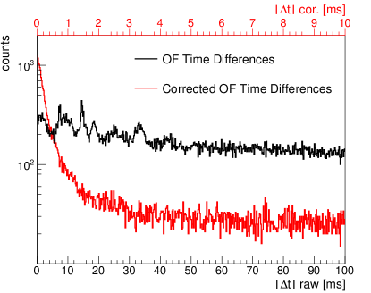
Figure 4: Time differences for $\mathcal{M}_{2}$ events whose energy sums to a prominent $\gamma$ peak in calibration data for both raw time (black) and corrected times (red). Note the time scales are different in the two cases to account for the much sharper peak with corrected times. Due to the high event rate in calibration data, an elevated rate of accidental coincidences is present leading to the presence of an elevated flat background in the $\Delta t$ distributions.

5 Data Selection Cuts and Blinding

After calibration is performed, the data are able to be meaningfully combined for analysis. We apply a set of simple “base” cuts to remove bad events. These cuts require that an event be flagged as a signal event (i.e, not a heater nor noise event), reject periods of bad detector operating conditions manually flagged due to excessive noise or environmental disturbances, reject any events with extremely atypical rise times, and reject any events with atypical baseline slope values. Additionally we reject all events from a single LMO that was observed to have an abnormally low signal-to-noise ratio which compromises its performance, as was done previously CuMoPRL . Beyond these base cuts, other improvements are possible with the use of more sophisticated selection cuts to remove background in order to increase the sensitivity to 0$\nu\beta\beta$ decay. We expect to observe background from:

• spurious / pileup events, suppressed with pulse shape discrimination cuts (see section 6);

• external $\gamma$ events, suppressed by removing multiple scatter events (see section 7);

• $\alpha$ background, removed using LD cuts (see section 8);

• $\beta$ events from close sources, suppressed by delayed coincidence cuts (see section 9);

• external muon induced events, removed with muon veto (see section 10).

Finally, we note that all cuts are tuned without utilizing data in the vicinity of $Q_{\beta\beta}$ (3034  keV) for ¹⁰⁰Mo. As was done previously CuMoPRL , we blind data by excluding all events in a 100  keV window centered at $Q_{\beta\beta}$. In the following sections we describe these selection cuts.

6 Pulse-Shape Discrimination

An expected significant contribution to the background near $Q_{\beta\beta}$ are pileup events in which two or more events overlap in time in the same LMO detector. This causes incorrect amplitude estimation and shifts events into our region of interest (ROI). In order to mitigate this effect we employ a pulse shape discrimination (PSD) cut that is comprised of two different techniques.

The main method we utilize for pulse-shape discrimination is based on principal component analysis (PCA), as was originally utilized in the previous analysis CuMoPRL ; PCA_Huang_2021 , and successfully applied recently to CUORE CUORE1ton with more details in Huang2021 . This method utilizes 2$\nu\beta\beta$ decay events between 1–2  MeV to derive a set of principal components that are used to describe typical pulse shapes for each channel-dataset. The leading principal component typically resembles an average pulse template with subsequent components adding small adjustments. These are used to compute a quantity referred to as the reconstruction error ($RE$) which characterizes how well a given pulse with $n$ samples, $\bm{x}$, is described by a set of $m$ principal components:

$$RE=\sqrt{\sum_{i=1}^{n}{\left(x_{i}-\sum_{k=1}^{m}{q_{k}w_{k,i}}\right)^{2}}},$$ (5)

where $\bm{w_{k}}$ is the $k$-th eigenvector of the PCA with the projection of $\bm{x}$ onto each component given by $q_{k}=\bm{x}\cdot\bm{w}_{k}$. $RE$ is energy dependent and this is corrected for by subtracting the linear component, $f(E)$, and normalizing by the median absolute deviation (MAD):

$$NE=\frac{RE-f(E)}{MAD}.$$ (6)

The resulting normalized reconstruction error, $NE$, is then used with an energy independent threshold to reject abnormal events.

6.1 PCA Improvements

We improve several aspects of the PCA cut compared to the previous implementation PCA_Huang_2021 : we utilize a cleaner training sample, perform normalization on a run-by-run basis, and correct for the energy dependence of the MAD. Abnormal pulses in the training sample result in distortions to all principal components leading to degraded performance in both efficiency and rejection power. To mitigate this we use a stricter selection cut requiring that the pretrigger baseline RMS not be identically zero (indicative of digitizer saturation and subsequent baseline jumps), and that a simple pulse counting algorithm must identify no more than one pulse on the LMO waveform and primary LD in the event window. This cleaner training sample allows us to utilize higher numbers of principal components without sacrificing efficiency.

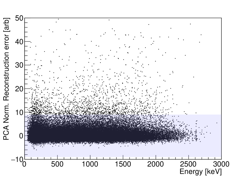
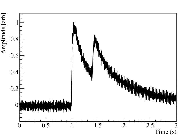
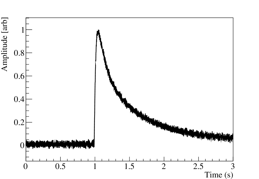
Figure 5: Example of the normalized PCA reconstruction error (left) as a function of energy, and two types of events (right) that exist in our data. (left:) The normalized reconstruction errors have no energy dependence and are normalized on a run-by-run basis for each channel allowing for a single energy independent cut to be applied across all channels in every dataset. Events with higher normalized reconstruction errors are removed and likely have incorrect energy values which may cause such events to be shifted into the region of interest. The shaded box denotes the acceptable normalized reconstruction error range for this cut. (right): The top event is an example of a pileup event with high normalized reconstruction error ($\sim$22) at $\sim$1189  keV which would have an incorrect amplitude reconstruction. The bottom event is a more typical pulse with a small normalized reconstruction error ($\sim$0.5) at $\sim$2482  keV, having no resulting error in its OF amplitude reconstruction.

By performing the normalization of $RE$ on a run-by-run basis, as opposed to whole-dataset, the fit for the linear component better reflects changes in $RE$ that may arise due to variations in noise. To correct for the energy dependence of the MAD, we require the aggregate statistics of a whole dataset. We perform a linear regression in energy and compute the average MAD of the ensemble. We then use the ratio of the linear regression function and ensemble average MAD as a correction to the individual channel MAD values, providing a proxy for a channel-dependent energy scaling of the MAD.

We examine the overall efficiency, impact on the 2615  keV $\gamma$ peak resolution, and optimization of the median discovery significance as suggested in Cowan et al. CowanMetric , as a function of number of PCA components and cut threshold. From this we choose to utilize the first 6 leading components of the PCA for this portion of the PSD cut. As seen in Fig. 5 the $NE$ quantity has no energy dependence and is able to reject obvious abnormal pulses.

6.2 PSD Enhancements

To finalize the PSD cut we utilize a two additional parameters developed in previous CUORE analyses CUOREPRL2017 . These parameters are computed on the optimally filtered pulse itself and are measures of goodness of fit on the left/right side of the filtered pulse, and are referred to as test-value-left and test-value-right (TVL and TVR) respectively. These $\chi^{2}$-like quantities are normalized via empirical fits of their median and MAD energy dependencies using $\gamma$ events between 500–2600  keV. As these quantities are computed on the filtered pulses they provide an additional proxy to detect subtle pulse-shape deviations and provide a complimentary way to reject pileup events, especially for noisy events PhysRevC.104.015501 .

We observe that some pileup events still leak through the six component PCA cut alone, primarily pileup with a short separation with the earlier pulse having a small amplitude relative to the “primary” pulse. Energy independent cuts on TVL and TVR are able to remove a large portion of these with negligible loss to efficiency. The discrimination power from these two cuts arises from the fact they are derived on the optimally filtered waveforms. They are sensitive to pileup in a fashion that the PCA is not, and owing to the better signal-to-noise ratio, tend reject small-scale pileup events that the PCA cut is insensitive to. We combine the various pulse-shape cuts to form the final PSD cut by requiring that the absolute value of the normalized reconstruction error be less than 9, and that the absolute value of the normalized TVR and TVL quantities each be less than 10. The resulting cut maintains an efficiency comparable to the previous analysis (see section 12) while being able to reject more types of abnormal events.

7 Anti-Coincidence

Due to the short range of ¹⁰⁰Mo $\beta\beta$ electrons in LMO (up to a few mm BandacBetaDepth ), 0$\nu\beta\beta$ decay events would primarily be contained within in a single crystal. A powerful tool to reduce backgrounds is to remove events where simultaneous energy deposits in multiple LMO crystals occur. It is useful to classify multi-crystal events for a background model and other analyses (e.g. $\beta\beta$ transitions to excited states). We define the multiplicity, $\mathcal{M}_{i}$, of an event by the total number of coincident crystals with an energy above 40  keV in a pre-determined time window. This requires measuring the relative times of events across different crystals. Previously we utilized a very conservative window of $\pm$100  ms, which due to the relatively fast 2$\nu\beta\beta$ decay rate in ¹⁰⁰Mo of $\sim 7\times 10^{18}$  yr or $\sim$2  mHz in a 0.2  kg ¹⁰⁰Mo-enriched LMO crystal CUPIDMo.2nu.precise , leads to $\sim$2% of single crystal ($\mathcal{M}_{1}$) events being accidentally tagged as two-crystal ($\mathcal{M}_{2}$) events. This results in a slight pollution of the $\mathcal{M}_{2}$ energy spectrum with these random coincidences as events that should be $\mathcal{M}_{1}$ have been incorrectly tagged as $\mathcal{M}_{2}$ events. The channel-channel time offset correction described in section 4.4 substantially narrows the $\Delta t$ distribution amongst channel-channel pairs allowing for a much shorter time window to be used (see Fig. 4). For this analysis we choose a coincidence window of 10 ms which reduces the dead time due to accidental tagging of $\mathcal{M}_{1}$ events as $\mathcal{M}_{2}$ by a factor of $\sim$10, while also producing a more pure $\mathcal{M}_{2}$ spectrum. The anti-coincidence (AC) cut then ensures we only examine single-crystal events.

8 Light Yield

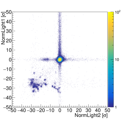
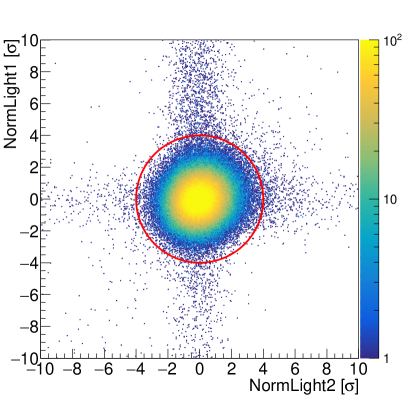
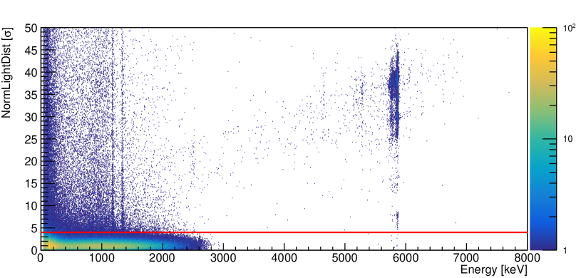
Figure 6: Two dimensional distribution of normalized light variables with LMO detector energy ¿1  MeV, zoomed out (top, left) and zoomed in (top, right) with the LY cut definition of $D<4$ also shown (solid circle). We observe that $\gamma/\beta$ signal like events are distributed around (0,0). The vertical band in the left figure is the result of a single light detector that has an excess ⁶⁰Co contamination resulting in a higher rate of events that deposit significant energy into this light detector. These are easily rejected with the light cut shown here as well as an anti-coincidence cut with the specific LD. Events populating the lower left quadrant are $\alpha$’s from the various detectors and show the hallmark deficiency of scintillation light on both light sensors. The energy dependence of the normalized light distance is shown in the bottom figure, again with the cut boundary denoted by a solid line. $\alpha$ events are clearly well separated from the $\beta$/$\gamma$’s. We observe that the norm light distance for these events is roughly flat with energy. The contamination due to excess ⁶⁰Co on 1 LD is evident. A cluster of $\alpha$ events at low normalized light distance is present due to a short period of time with sub-optimal performance on a single LD.

LDs are the primary tool we use in CUPID-Mo to distinguish $\alpha$ from $\beta/\gamma$ particles to reduce degraded $\alpha$ backgrounds. Using the detected LD signal relative to energy deposited in the LMO detector, we are able to separate $\alpha$’s from $\beta/\gamma$ events as the former have $\sim$20% the light yield of the latter for the same heat energy release. Previously, we exploited the information provided from the LDs by using a resolution-weighted summed quantity and direct difference to select events with light signals consistent with $\beta/\gamma$’s CuMoPRL . In this analysis we modify the light cuts to utilize the correlation between both LDs associated with an LMO detector more directly. To account for the energy dependence of the light cut, we model the light band mean and width. We divide the light band into slices in energy for each channel and dataset. For each slice we perform a Gaussian fit of the LD energies to determine the mean and resolution, then fit the means to a second order polynomial in energy, and the resolutions to:

$$\sigma(E)=\sqrt{p_{0}^{2}+p_{1}\cdot E}.$$ (7)

This is used to determine the best estimate of the expected LD energy for a given energy. We define the normalized LD energy for a given LMO detector $c$ in dataset $d$ as:

$$n_{c,s,d}=\frac{L_{c,s,d}-\widehat{L}_{c,s,d}(E)}{\sigma(E)_{c,d,s}},$$ (8)

where $s$ is the LD neighbor index, $L_{c,s,d}$ is the measured LD energy, $\widehat{L}_{c,s,d}(E)$ is the expected LD energy, and $\sigma_{c,d,s}(E)$ is the expected width of the light band. This procedure explicitly removes the energy dependence, and we note that $n_{c,s,d}$ has a normal distribution.

We expect signal-like $\beta/\gamma$ events to have similar energies on the both LDs CuMo_instrument . We observe background events where the total light energy is consistent with $\beta/\gamma$ signal events but the resulting individual LD energies are very different. This can happen due to surface $\alpha$ events where a nuclear recoil deposits some energy onto only one LD (see lumineu2017 ), or contamination on the LDs themselves. To remove these background-like events we exploit the full information of two LDs by making a two-dimensional light cut. In particular, we expect the joint distribution of $n_{c,0,d}$ and $n_{c,1,d}$ to be a bivariate Gaussian. This is also observed in data, with minimal correlations between the two normalized LD energies, thus a simple radial cut can be defined by computing the normalized light distance, $D_{c,d}$:

$$D_{c,d}=\sqrt{n_{c,0,d}^{2}+n_{c,1,d}^{2}}.$$ (9)

For channels which do not have two LDs we instead make a simple cut on the single normalised light energy which is available. We chose a cut of $D<4$ (corresponding to $\sim 3.5\sigma$ equivalent coverage). As shown in Fig. 6 this is sufficient to remove the $\alpha$ background which is characterized by a large negative value of $n_{c,s,d}$.

9 Delayed Coincidences

A significant background for calorimeters can be surface and bulk activity in the crystals themselves due to natural U/Th radioactivity (see Denys.Andrea.LTD for more details). In particular, because $Q_{\beta\beta}$ of ¹⁰⁰Mo (3034  keV) is above most natural radioactivity, the only potentially relevant isotopes are ²⁰⁸Tl, ²¹⁰Tl and ²¹⁴Bi PirroScintBolo . However, given both the low contamination in the CUPID-Mo detectors and the very small branching ratio ($\sim$0.02%), the decay chain of ²¹⁴Bi $\rightarrow$ ²¹⁰Tl $\rightarrow$ ²¹⁰Pb is negligible.

For ²⁰⁸Tl the decay chain proceeds as:

$${}^{212}\text{Bi}\xLongrightarrow[\alpha(6207~{}\,\text{keV})]{60.6~{}\,\text{min},\ \ 35.9\%\ \text{BR}}\ ^{208}\text{Tl}\xLongrightarrow[\beta^{-}(4999~{}\,\text{keV})]{3.1~{}\,\text{min},\ \ 100\%\ \text{BR}}\ ^{208}\text{Pb}.$$ (10)

A common approach is to reject candidate ²⁰⁸Tl events that are preceded by a ²¹²Bi $\alpha$ decay PirroScintBolo ; CUPID0Final . We note that for bulk activity, the candidate $\alpha$ is detected with $>99$% probability, so it is the efficiency at which these $\alpha$ events pass the analysis cuts that sets this background. For surface $\alpha$ events, $\sim$50% reconstruct at their $Q$-value, so a delayed coincidence cut would remove only about $\sim$50% of surface events (see CUPID0Final ). In this analysis we use the same energy and time difference as was used previously CuMoPRL : we reject any candidate ²⁰⁸Tl event that is within 10 half-lives from a ²¹²Bi candidate event. We note that the CUPID-Mo detector structure with a reflective foil and Cu holder surrounding each crystal reduces the effectiveness of this cut for surface events. In a future experiment with an open structure (for example CUPID CUPID:2019 , CROSS CROSS , or BINGO Nones2021 ) the detection of multi-site $\alpha$ events may significantly improve this detection probability (and therefore cut rejection).

Table 1: Energy and time selections used for CUPID-Mo delayed coincidence cuts

Cut	$Q_{\alpha}\ \mathrm{[keV]}$	Energy cut [keV]	Time [s]
212Bi 208Tl	$6207$	$6000-6300$	1830
222Rn 214Bi	$5590$	$5490-5620$	13860
218Po 214Bi	$6115$	$6015-6565$	13620

In addition to this commonly used cut, the extremely low count rate for $\alpha$’s in CUPID-Mo, due to low contamination Schmidt2020 ; Poda2020 , enables a novel extended delayed-coincidence cut designed to remove potential ²¹⁴Bi induced events. We focus on the lower part of the decay chain:

$$\begin{split}&{}^{222}\text{Rn}\xLongrightarrow[\alpha(5590~{}\,\text{keV})]{3.8~{}\,\text{day},\ \ 100\%\ \text{BR}}\ ^{218}\text{Po}\xLongrightarrow[\alpha(6115~{}\,\text{keV})]{3.1~{}\,\text{min},\ \ 99.98\%\ \text{BR}}\ ^{214}\text{Pb}\\ &{}^{214}\text{Pb}\xLongrightarrow[\beta^{-}(1018~{}\,\text{keV})]{27.1~{}\,\text{min},\ \ 100\%\ \text{BR}}\ ^{214}\text{Bi}\xLongrightarrow[\beta^{-}(3269~{}\,\text{keV})]{19.7~{}\,\text{min},\ \ 99.98\%\ \text{BR}}\ ^{214}\text{Po}\\ &{}^{214}\text{Po}\xLongrightarrow[\alpha(7834~{}\,\text{keV})]{163.4~{}\,\mu\text{s},\ \ 100\%\ \text{BR}}\ ^{210}\text{Pb}\end{split}$$ (11)

We tag the ²¹⁴Bi nuclei based on either the ²²²Rn or ²¹⁸Po $\alpha$ decay. Compared to ²¹²Bi $\rightarrow$ ²⁰⁸Tl coincidences, a much larger veto time window is required. We set these time cuts based on a simulation of the time differences between decays in order to have a 99% probability of the decay being in the selected time range, as shown in Table 1. We veto events where there is an $\alpha$ candidate within [$Q_{\alpha}-$100, $Q_{\alpha}$+50]  keV and within the time differences in Table 1 in the same LMO detector. This energy range is chosen to fully cover the $Q$-value peaks. Despite the dead time per event being large, the total dead time is acceptable ($<1\%$, see section 12) thanks to the low contamination of ²²⁶Ra in the CUPID-Mo detectors. We observe several events with $E>2600$ keV that are rejected, while the events removed at lower energy are dominated by accidental coincidences of 2$\nu\beta\beta$ decays.

10 Muon veto coincidences

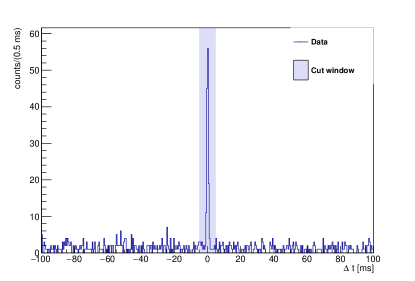
Figure 7: Time differences between muon veto and LMO detector events after we have subtracted off the peak offset ($\sim 60$ ms). The cut of $\pm 5$ ms is used in our analysis. To obtain a good signal-to-noise ratio, only events with $\mathcal{M}>1$ in the LMO detectors are selected.

We apply an anti-coincidence cut between the LMO detectors and an active muon veto to reject prompt backgrounds from cosmic-ray muons which may deposit energy in the ROI, with LY similar to a $\gamma/\beta$. The muon veto system is described in detail in SCHMIDT201328 . We utilize muon veto timestamps to compute an initial set of coincidences between LMO detectors and the veto system. We observe a clear $\Delta t$ peak of muon induced events which we correct for (see Fig. 7). The muon veto coincidences are then defined using the corrected times with a window of $\pm$ 5  ms. The relatively small window removes the need to also place a requirement on the number of muon veto panels triggered, maximizing the rejection of background events with minimal impact on livetime.

11 Energy spectra

After all cuts are tuned on the blinded data we proceed to compute cut efficiencies, extract the resolution energy scaling, energy bias, and define the ROI. The application of successive cuts can be seen in Fig. 8. Starting with the base cuts, the application of the PSD cuts produces a spectrum of events originating from real physical interactions with the detector (i.e., devoid of abnormal events). We see that the spectrum is dominated by 2$\nu\beta\beta$ decay from $\sim$1 MeV up towards $Q_{\beta\beta}$ with few events populating the $\alpha$ region. The application of the AC cuts removes only a small amount of events as the majority of events are single-crystal interactions. The most significant selection cut is the application of the LY cut which removes almost all remaining events at high energies where degraded $\alpha$ events may be present.

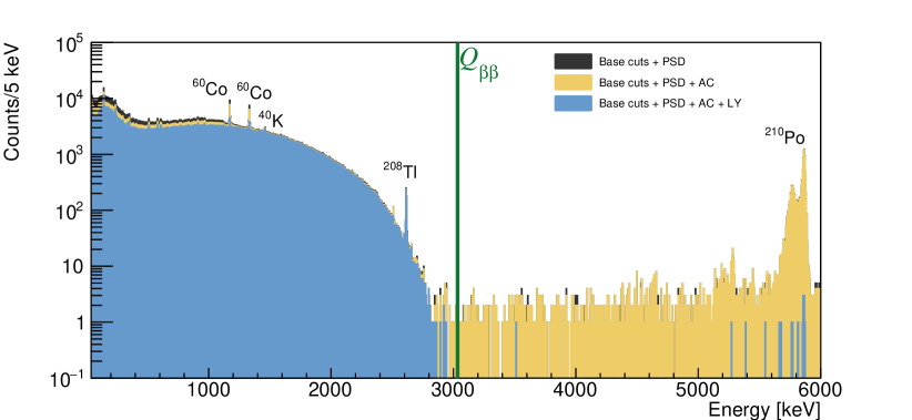
Figure 8: Unblinded spectrum of physics data in CUPID-Mo with successive application of cuts. The application of the PSD cuts produces a spectra containing all events with good pulse shape characteristics. Application of the anti-coincident (AC) cut removes all events with multiplicity greater than one, along with any possible delayed coincidences from ²¹²Bi, ²²²Rn, or ²¹⁸Po decay chains, and any events coincident with the muon veto. The final application of the light cut removes almost all the high energy background induced from degraded $\alpha$’s that remains, leaving a few intermediate LY events at high energy. The large green vertical line indicates the location of $Q_{\beta\beta}$ (3034  keV).

12 Efficiencies

In order to compute the cut efficiencies we use three methods that span the distinct types of cuts present in this analysis:

• noise events for pileup efficiency;

• efficiency from $\gamma$ peaks;

• efficiency from ²¹⁰Po peak.

Table 2: Efficiencies for CUPID-Mo selection cuts, evaluated either as a constant efficiency or linearly extrapolated to $Q_{\beta\beta}$. Methods used to compute each efficiency are indicated (see text)

Cut	Efficiency Flat / $Q_{\beta\beta}$ [%]	Method
Pileup	$95.7\pm 1.0$	Noise
Anti-coincidence	$99.55\pm 0.07$	210Po
Muon veto	$99.62\pm 0.07$	210Po
Delayed coincidence	$99.16\pm 0.01$	210Po
PSD	$95.2\pm 0.5/94.3\pm 1.5$	$\gamma$ peaks
Light Distance	$99.4\pm 0.4/99.7\pm 0.8$	$\gamma$ peaks
Total Analysis Efficiency	88.4 $\pm$ 1.8	-

We note that the trigger efficiency for this analysis is taken as 100%. The typical 90% trigger thresholds are $\sim$8.5  keV and $\sim$0.55  keV for LMO detectors and LD’s respectively, well below the 40  keV analysis threshold used by the anti-coincidence cuts. The trigger efficiencies are measured by injecting scaled pulse templates into actual noise events and running these through the optimum trigger for each channel-dataset pair. More details of this process are described in helisThesis (Sect. 3.3.2).

The pileup efficiency is the probability that an event will not have another pulse in the same time window during which event reconstruction takes place. In addition, we check if the energy of the noise event is biased by $>$ 20 keV. If either of these two possibilities occur, we consider the event a pileup. We compute the pileup rejection efficiency as the ratio of the noise events passing the single trigger criterion and with energy inside $\pm$20  keV to the total number of noise events. We present the exposure weighted average over all datasets in Table 2 and assign a 1% uncertainty to this calculation due to the extrapolation from noise to physics events. We note that this is equivalent to a statistical calculation based on the known trigger rate, but this method averages over varying trigger rates (in time or across channels).

The anti-coincidence, delayed coincidence, and muon veto cuts are not expected to have energy dependent efficiencies and represent detector deadtimes. For each of these we evaluate the efficiency utilizing events in the ²¹⁰Po $Q$-value peak at 5407  keV, as this peak has a very high energy and provides a clean sample of physical events. We extract the efficiency as $\varepsilon=N_{\text{pass}}/N_{\text{total}}$ integrating in a $\pm$50 keV window around the peak; the results are listed in Table 2.

We compute the efficiency of the normalized light distance cut (i.e., LY cut) and the PSD cut using a new method in this analysis. We fit the $\gamma$ peaks in the $\mathcal{M}_{1}$ data as they provide a clean sample of signal-like events, and are a more robust population with which to evaluate the efficiency, compared to using all physics events as was done previously CuMoPRL . In order to account for background with non-signal like events around each peak we fit the distributions of both events passing and failing each cut to a Gaussian plus linear model. The efficiency is then given as:

$$\varepsilon=N_{\text{pass}}/(N_{\text{pass}}+N_{\text{fail}}).$$ (12)

We do not expect large variation in the cut efficiency across datasets and in order to maintain sufficient statistics when using the $\gamma$ peaks we compute only the global cut efficiencies. We estimate the uncertainty numerically by sampling from the uncertainty on the number of events in the photopeaks from the Gaussian fit. We apply the LY cut in order to gain a clean sample of events when measuring the PSD efficiency and vice-versa, which is possible due to the independence of the heat and normalized light signals. We perform this for each significant $\gamma$ peak in the $\mathcal{M}_{1}$ physics data (excluding the ⁶⁰Co peaks for the LY cut as they are known to be biased due to a contaminated LD). We fit the efficiency as a function of peak energy to a linear polynomial and observe that the efficiency is consistent with being constant (between 238–2615  keV). We extrapolate to $Q_{\beta\beta}$ in order to obtain the efficiencies for each cut in order to account for any systematic energy dependence. These fits are shown in Fig. 9.

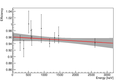
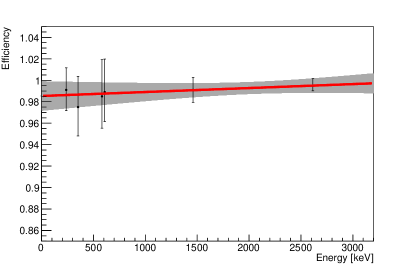
Figure 9: Plot showing the efficiency for the PCA cut (Upper) and normalized light distance cut (Lower) obtained from $\mathcal{M}_{1}$ $\gamma$ peaks as a function of the peak energy (back points). We fit these graphs to a linear polynomial (red line) and the confidence interval of this linear fit is shown in gray.

We combine the efficiencies measured in Table 2 to determine the overall total analysis efficiency. We sample from the errors for each efficiency (assumed to be Gaussian), and obtain an estimate of the probability distribution of the total efficiency from which we extract the analysis cut efficiency with a Gaussian fit as $\varepsilon=$ (88.4 $\pm$ 1.8)%.

13 Resolution Scaling and Energy Bias

As there is no significant naturally occurring $\gamma$ peak near $Q_{\beta\beta}$ we must perform an extrapolation of the resolution as a function of energy and likewise for the energy scale bias. In order to account for variations in the performance and noise of each LMO detector over time, we obtain the energy scale extrapolations on a channel-dataset basis. Due to the excellent radiopurity and the relatively fast 2$\nu\beta\beta$ decay rate which covers most $\gamma$ peaks in the spectrum, we cannot determine this scaling directly from physics data alone. In order to have sufficient statistics, we utilize calibration data to obtain a lineshape from the 2615  keV $\gamma$ events which is then extrapolated to physics data.

13.1 Resolution in Calibration Data

As in CuMoPRL we perform a simultaneous fit of the 2615 keV peak in calibration data for each dataset. This fit is an unbinned extended maximum likelihood fit implemented using RooFit RooFit . We model the data in each channel as:

$$f_{c,d}(E)=N_{c}( p_{b}\cdot f_{b}(E;l)$$ (13)

$$+p_{s}\cdot f_{s}(E;\mu_{c,d},\sigma_{c,d})$$

$$+f_{g}(E;\mu_{c,d},\sigma_{c,d}))$$

where $c$ is the channel number, $d$ is the dataset and the functions $f_{b}(E;l),f_{s}(E;\mu_{c,d},\sigma_{c,d}),f_{g}(E;\mu_{c,d},\sigma_{c,d})$ are normalized linear background, smeared step and Gaussian functions. The parameter $l$ is the slope of the linear background, $\mu_{c,d}$ is the mean of the peak for channel $c$ in dataset $d$ and $\sigma_{c,d}$ is the corresponding standard deviation. $p_{b},p_{s}$ are the background and smeared step ratio (these parameters are shared for all channels). $N_{c}$ is the number of events in the Gaussian peak, while $\sigma_{c},\mu_{c}$ are the resolution and mean for this channel. An example of one of these fits is seen in Fig. 10. We observe in each dataset that the core of the peak is well described by the model with some distortion in the low-energy tail due to the presence of pileup events due to the high event rate in calibration data. We use the individual channel-dataset widths and means in the physics data extrapolation.

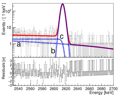
Figure 10: Simultaneous fit of calibration data 2615  keV $\gamma$ peak, and residuals for all channels in a single dataset with Poisson errors in each bin. Top: the summed total effective fit components (dashed blue lines) are labeled. Component (a) is the total excess background modeled by a linear fit, component (b) is the sum of Gaussian lineshapes used for each channel, and component (c) is the smeared step function to represent multi-Compton background. The simultaneous fit is shown as a solid line. Bottom: the residuals of the fit showing overall excellent agreement across the model with the central core well described.

13.2 Resolution in Physics Data

In order to reconstruct the resolution in physics data we use a slightly different procedure compared to CuMoPRL and CUOREPRL2020 . We fit selected peaks with the lineshape model and extract an energy dependent resolution function from this. In the previous analysis we utilized a simple Gaussian plus linear background for each peak fit on the total summed spectrum and took the ratio, $R$, of each peak resolution to the calibration summed spectrum 2615  keV $\gamma$ peak. Here we introduce a new exposure weighted lineshape function:

$$f(E)=\sum_{d=1}^{9}\sum_{c=1}^{19}\frac{(Mt)_{c,d}}{Mt}f_{g}(E;\mu,\sigma_{c,d}\cdot R),$$ (14)

where the summation occurs over channels $c$, and datasets $d$, $Mt$ is the exposure, $f_{g}(E)$ is a Gaussian, $\mu$ is the mean of the peak and $R$ is a ratio scaling from calibration to physics data. We fit each peak in the physics data summed spectrum to this lineshape plus a linear background as a binned likelihood fit with the number of events in the peak, and the linear background, $R$ and $\mu$ as free parameters.

After all peaks in physics data have been fit we can model the resolution ratio as a function of energy. A typical functional form for the resolution of a calorimeter can be given by:

$$\sigma(E)=\sqrt{\sigma_{0}^{2}+p_{1}E},$$ (15)

where the term $\sigma_{0}$ is related to the baseline noise in the detector, while $p_{1}$ characterizes any stochastic effects that degrade the resolution with increasing energy, as in lumineu2017 . We use noise events to constrain the baseline component of the energy resolution. By fitting the distribution of noise events to the same model as the physics peaks we measure $R(0\ \mathrm{keV})$. We fit $R(E)$ for each physics peak and also the noise peak to Eq. 15 as shown in Fig. 11. As in the previous analysis, we also considered a simple linear model, $\sigma=p_{0}+p_{1}E$ for the resolution scaling. Previously, in physics data there were insufficient statistics to favor one model over another, however with the additional two datasets this linear model is disfavored, as has been seen in calibration data.

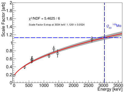
Figure 11: Resolution scaling fit showing the scaling factor $R$, between background and calibration data for each peak in physics data. We model this as $R(E)=\sqrt{p_{0}^{2}+p_{1}E}$ and extrapolate to $Q_{\beta\beta}$ to obtain a global scale factor. The choice of functional form derives from the energy resolution scaling in data following this same functional form.

Using the model in Eq. 15 we extrapolate the ratio at $Q_{\beta\beta}$ to be $R(3034~{}\,\mathrm{keV})=$ $1.126\pm 0.052$. This number then is used to scale each of the channel-dataset dependent 2615  keV resolutions from the simultaneous lineshape fit in calibration data to resolutions at $Q_{\beta\beta}$ in physics data:

$$\begin{split}&\sigma_{c,d}(Q_{\beta\beta})=R(Q_{\beta\beta})\cdot\sigma_{c,d}\pm\\ &\sqrt{(R(Q_{\beta\beta})\cdot\sigma(\sigma_{c,d}))^{2}+(\sigma(R(Q_{\beta\beta}))\cdot\sigma_{c,d})^{2}}.\end{split}$$ (16)

These extrapolated resolutions are used to compute the containment efficiency (see section 12). The exposure weighted harmonic mean of the 2615  keV line in calibration data is $\left(6.6\pm 0.1\right)$  keV FWHM. We use this to compute the effective resolution in physics data at $Q_{\beta\beta}$ by scaling by $R(3034~{}\,\mathrm{keV})$, obtaining $(7.4\pm 0.4)~{}\,\mathrm{keV}$ FWHM.

13.3 Energy Bias

The total effective energy bias is also extracted from the fit done in physics data described in section 13.2. Using the best fit peak locations, $\mu$ from the lineshape fit (Eq. 14), we fit the residuals of $\mu-\mu_{\text{lit.}}$ as a function of $\mu_{\text{lit.}}$ to a second order polynomial as shown in Fig. 12. As in the previous analysis, we find the distribution is well described by this model and we extract the energy bias at $Q_{\beta\beta}$ as $E-Q_{\beta\beta}=$ $(-0.42\pm 0.30)~{}\,\mathrm{keV}$.

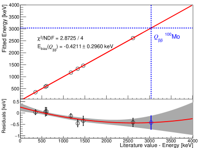
Figure 12: Energy bias in physics data. Here the best fit central value vs true value for each peak in the physics data is fit against a quadratic polynomial. The residual evaluated at $Q_{\beta\beta}$ is then obtained from this fit giving an estimate for the energy scale bias.

14 Bayesian Fit

14.1 Model Definition

We use a Bayesian counting analysis to extract a limit on $T_{1/2}^{0\nu}$, similar to that in CuMoPRL . However, due to significant improvements in the background modelling of the CUPID-Mo data we modify this analysis. We model our background in the ROI as the sum of an exponential and linear background:

$$f(E)=B\cdot\Big{(}\frac{p_{f}}{\Delta E}+(1-p_{f})\cdot\frac{e^{-(E-Q_{\beta\beta})/\tau}}{N}\Big{)},$$ (17)

where $B$ is the total background index (averaged over the 100 keV blinded region) in $\mathrm{counts/(keV\cdot kg\cdot year)}$, $\Delta E$ is the width of the blinded region (100 keV), $\tau$ is the slope of the exponential and $p_{f}$ is the probability of flat background. Finally, $N$ is a normalization factor for the exponential. We use a counting analysis with three bins, with the expected number of counts in a bin with index $i$ given by:

$$\lambda_{i}=\sum_{c=1}^{19}\sum_{d=1}^{9}(Mt)_{c,d}/Mt\cdot\Big{(} \varepsilon_{i}(c,d)\cdot\Gamma^{0\nu}\frac{N_{A}\cdot Mt\cdot\eta}{W}$$ (18)

$$+\int_{E_{a,i}(c,d)}^{E_{b,i}(c,d)}f(E)dE\Big{)}.$$

The sum $c$ is over all channels and $d$ over all datasets. $\Gamma^{0\nu}$ is the $0\nu\beta\beta$ decay rate, $N_{A}$ is Avogadro’s number, $Mt$ is the total LMO exposure, while $(Mt)_{c,d}$ is the exposure for one channel/dataset, $\eta$ is the isotopic enrichment, and $W$ is the enriched LMO molecular mass. $\varepsilon_{i}(c,d)$ is the total $0\nu\beta\beta$ decay detection efficiency for channel $c$, dataset $d$, and bin $i$. This is the product of the analysis efficiency (see section 12) and the containment efficiency. This is the probability for a $0\nu\beta\beta$ decay event to have energy in bin $i$ and to be $\mathcal{M}_{1}$. The expected number of counts is a sum of a signal contribution $\varepsilon(c,d)\cdot N^{0\nu}$, and a background contribution from integrating $f(E)$ between the bounds $[E_{a,i}(c,d),E_{b,i}(c,d)]$, the upper and lower bounds for the bin $i$. The decay rate is normalized by a constant to give the number of 0$\nu\beta\beta$ decay events. The three bins used in this analysis represent lower/upper side-bands to constrain the background, and a signal region. The energy ranges of the signal region are chosen on a channel-dataset basis (see section 14.2), and the remaining energies out of the 100 keV fit region form the sidebands. The efficiencies $\varepsilon(c,d)$ are defined for each detector-dataset from Monte Carlo (MC) simulations accounting for the energy resolution and its uncertainty. Our likelihood is then given by a binned Poisson likelihood over three bins:

$$\mathcal{L}=\prod_{i=0}^{2}\frac{\lambda_{i}^{N_{i}}e^{-\lambda_{i}}}{N_{i}!}.$$ (19)

We simultaneously minimise and sample from the joint posterior distribution using the Bayesian Analysis Toolkit (BAT BATCaldwell ). Our model parameters are:

• $B$: the background index;

• $p_{f}$: the probability of flat background;

• $\tau$: the exponential background decay constant;

• $\Gamma^{0\nu}$: the $0\nu\beta\beta$ decay rate.

We also include systematic uncertainties as nuisance parameters as described in section 14.5.

14.2 Optimization of the ROI

Due to the different performance of each channel across datasets we use different ROIs for each. These are optimized using blinded data to maximize the mean expected sensitivity using the same procedure defined in CuMoPRL . We optimize the ROI window based on the likelihood ratio defined as:

$$R(c,d,E)=\frac{\mathcal{L(B)}}{\mathcal{L}(S)},$$ (20)

where $\mathcal{L}(B)$ is the probability that an event at energy $E$ in channel $c$ and dataset $d$ is background, and $\mathcal{L}(S)$ is the same for signal. We divide the energy in 0.1  keV bins between 2984–3084  keV for each channel-dataset from which we extract the containment efficiency and estimated background. We rank these bins via the likelihood ratio:

$$R(c,d,E_{i})=\frac{\mathcal{L(B)}}{\mathcal{L}(S)}\propto\frac{\varepsilon_{c,d,E_{i}}}{B_{c,d,i}},$$ (21)

where the background index is assumed to be constant at $5\times 10^{-3}$ $\mathrm{counts/(keV\cdot kg\cdot year)}$ (in the previous analysis we found this assumption does not significantly impact the results CuMoPRL ). We then optimize the choice of the maximum allowed likelihood ratio to include by maximizing the mean limit setting sensitivity, as a Poisson counting analysis:

$$S=\sum_{n=0}^{3}p(n)\cdot S(n),$$ (22)

with the limit, $S(n)$, of 2.3 counts in the case of zero events, 3.9 for one event, etc., and $p(n)$ is the probability of observing $n$ counts based on the expected background rate. The chosen channel-dataset based ROIs are shown in Fig. 13, with an exposure weighted effective ROI width of $(17.1\pm 4.5)$  keV, corresponding to ($2.3\pm 0.6$) FWHM at $Q_{\beta\beta}$.

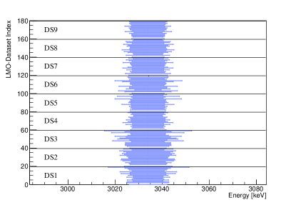
Figure 13: Summary plot of the ROI width for every channel-dataset in this analysis. Horizontal lines demarcate each of the nine separate datasets and blue lines are a particular channel’s ROI. The x-axis range spans the entire 100 keV blinded region.

14.3 Containment Efficiency

Once the channel-dataset based ROIs have been chosen we can compute the containment efficiency for each channel and dataset pair. This efficiency is evaluated using Geant4 MC simulations, accounting for the energy resolutions extracted in section 13. The average containment efficiency is ($75.9\pm 1.1$)%. To estimate the systematic uncertainty from the MC simulations we vary the simulated crystal dimensions and Geant4 production cuts resulting in a $1.5\%$ relative uncertainty.

14.4 Extraction of the Background Prior

The most significant prior probabilities in our analysis are for the signal rate $\Gamma^{0\nu}$ and the background index $B$. Due to the very low CUPID-Mo backgrounds and a relatively small exposure, data around the ROI does not constrain $B$ well. However, detailed Geant4 modelling does provide a measurement of the background averaged over our 100  keV blinded region (a forthcoming publication on the background modelling is in preparation). This fit models our experimental data in bin $i$ as (in units of counts/keV):

$$\mu_{i}=\sum_{j=1}^{k}N^{\text{MC}}_{j,i}\cdot f_{j}/\Delta E,$$ (23)

where the sum is over all simulated MC contributions, $N^{\text{MC}}_{j,i}$ is the number of events in the simulated MC spectra $j$ and bin $i$, and $f_{j}$ is a factor we obtain from the fit. This fit is performed using a Bayesian fit based on JAGS JAGS_Proceeding ; JAGS3 , similar to CUORE.2nu ; CUPID0.BM . It estimates the joint posterior distribution of the parameters $f_{j}$, and we sample from this distribution at each step in the Markov chain computing:

$$B_{i}=\sum_{j=1}^{k}\frac{N^{\text{MC}}_{j,i}\cdot f_{j}}{Mt}.$$ (24)

From the marginalized posterior distribution of the observable background index we obtain:

$$\mbox{$B$ = {\color[rgb]{0,0,0}{$\left(4.7\pm 1.7\right)\times 10^{-3}$}}~{}\,$\mathrm{counts/(keV\cdot kg\cdot year)}$}.$$ (25)

This value is used as a prior in our Bayesian fit with a split-Gaussian distribution; two Gaussian distributions with the same mode are combined such that values on either side of the mode have different variances. We have found that in the case of observing zero events, this prior does not change the observed limit. However, if some events are observed, this is a more conservative choice than a non-informative flat prior since it prevents the background index from floating to high values that are strongly disfavored by the background model.

To extract a prior on the slope of the exponential background, $\tau$, we perform a fit to the blinded data (between $2650$ to $2980$ keV) to a constant plus exponential model, as seen in Fig. 14. This results in a best fit of $\tau=\left(65.7\pm 4.6\right)\ \mathrm{keV}$, which is used as a prior in our analysis. The probability of the background being uniform (instead of exponential) is given a uniform prior between $[0,1]$.

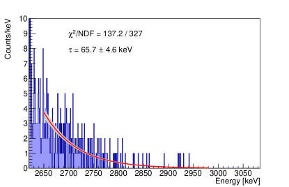
Figure 14: The exponential plus flat background fit used to determine a prior on the slope of any exponential background. The fit favors an exponential term with no flat background, however owing to the low statistics it is not sufficient to rule out the presence of a flat background term.

14.5 Systematic Uncertainties

We include systematic uncertainties in our Bayesian fit as nuisance parameters, in particular we account for uncertainties in:

• cut efficiencies;

• isotopic enrichment;

• containment efficiency.

These are each given Gaussian prior distribution with the values from sections 12 and 13 as indicated in Table 3.

Table 3: Nuisance parameters for the Bayesian model and their central values and prior type. The background index has an asymmetric uncertainty and is treated as a split-Gaussian, with each side corresponding to the different asymmetric uncertainty values. The signal rate is treated as a uniform prior in the positive domain.

Nuisance Parameter	Value	Prior type
Rate	[0, $40\times 10^{-24}$]  yr-1	Uniform
Isotopic Enrichment	$0.966\pm 0.002$	Gauss.
0$\nu\beta\beta$ decay containment (MC)	$1.000\pm 0.015$	Gauss.
Analysis Efficiency (global)	$0.8843\pm 0.0180$	Gauss.
Background Index	$(4.7^{+1.7}_{-1.7})\times 10^{-3}$ $\mathrm{counts/(keV\cdot kg\cdot year)}$	Split Gauss.
Probability of flat background ($p$)	[0, 1]	Uniform
Exponential background slope ($\tau$)	$\left(65.7\pm 4.6\right)$  keV	Gauss.

As in CuMoPRL these uncertainties are marginalized over and are automatically included in our limit. We note that the systematic uncertainties from the energy bias and resolution scaling are incorporated in the computation of the containment efficiency. We chose a uniform prior on the rate, $\Gamma^{0\nu}\in[0,40\times 10^{-24}$]  yr^-1. This is consistent with the standard practice for 0$\nu\beta\beta$ decay analysis GERDA2020 ; EXO200.2019 ; CUORE1ton . The range is large enough that it has minimal impact on the possible result, and provides as little information as possible on the rate to avoid possible bias.

15 Results

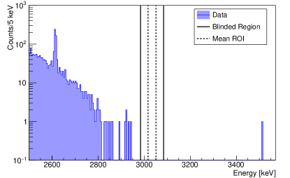
Figure 15: The unblinded background spectrum near the ROI for 2.71  kg$\times$year of data (1.47  kg$\times$year for ¹⁰⁰Mo). After application of all cuts we observe no events in both the ROI and in the full 100  keV blinded region. In this work, the event near 3200  keV present in the previous analysis CuMoPRL , was tagged as coincident with the improved muon veto. The exposure weighted mean ROI (17.12  keV) is shown with dashed lines, and the full blinded region is within the solid lines.

After unblinding our data, we observe zero events in the channel-dataset ROIs and zero events in the side-bands, as shown in Fig. 15. This leads to an upper limit on the decay rate $\Gamma^{0\nu}$ including all systematics of:

$${\color[rgb]{0,0,0}{\Gamma^{0\nu}<3.8\times 10^{-25}\ \mathrm{year^{-1}}\ \text{(stat.+syst.})\ \text{at 90\% C.I.}}}$$ (26)

or:

$$T_{1/2}^{0\nu}>{\color[rgb]{0,0,0}{1.8}}\times 10^{24}~{}\text{year}\ \text{(stat.+syst.)}\ \text{at 90\% CI.}$$ (27)

This limit surpasses our first result of $T^{0\nu}_{1/2}>1.5\times 10^{24}$  yr CuMoPRL , becoming a new leading limit on 0$\nu\beta\beta$ decay in ¹⁰⁰Mo. The posterior distribution of the decay rate is shown in Fig. 16. We find that this can be fit well by a single exponential as expected for a background-free measurement. We extract:

$$p(\Gamma^{0\nu}|D_{\text{CUPID-Mo}})=\lambda\cdot e^{-\lambda\cdot\Gamma^{0\nu}}d\Gamma^{0\nu},$$ (28)

where

$${\color[rgb]{0,0,0}{\lambda=(6.061\pm 0.001)\times 10^{24}\ \mathrm{year}}},$$ (29)

and $D_{\text{CUPID-Mo}}$ is the CUPID-Mo data.

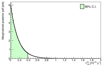
Figure 16: The posterior distribution of the decay rate for 0$\nu\beta\beta$ decay run with all nuisance parameters floating. The shaded area under the curve represents the 90% C.I. with upper limit at a value of $\Gamma^{0\nu}$ = $3.8\times 10^{-25}\ \mathrm{y^{-1}}$.

We can extract the 90% C.I. on the signal counts from the posterior, resulting in an upper limit of $S<2.3$ counts (90% C.I.), consistent with what one would expect from a Poisson counting experiment with zero observed events. Our Bayesian analysis leads to a non-zero background index in the 100  keV fit region with a 1$\sigma$ interval of:

$$\mbox{$B$ = {\color[rgb]{0,0,0}{$\left(3.9^{+1.7}_{-1.6}\right)\times 10^{-3}$}}~{}\,$\mathrm{counts/(keV\cdot kg\cdot year)}$}.$$ (30)

This is mostly consistent with the informative background model prior. Further studies are ongoing to include extra information into the background model fit (i.e. constraints on pileup from simulation or calibration data) to reduce this uncertainty. The posterior distributions for the exponential background parameters are consistent with the priors derived from the fit of the 2$\nu\beta\beta$ decay spectrum in an energy interval between 2650$-$2980  keV (as done previously CuMoPRL ).

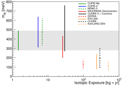
Figure 17: Published $\left<m_{\beta\beta}\right>$ values as a function of isotopic exposure for several experiments Q0FinalPRC ; CUPID0Final ; NEMO30vMo ; MJD2019 ; EXO200.2019 ; GERDA2020 ; CUORE1ton ; KamLANDZen2016 . While each experiment has utilized different sets of nuclear matrix elements, the published results represent a standard set of values we can compare this work’s result to. The spread for CUPID-Mo results is shown with a band for illustrative purposes only, indicating the $\left<m_{\beta\beta}\right>$ range as it relates to other experiments more clearly and showing the promise of this technology with only a relatively modest isotopic exposure.

In order to study the effect of systematics we perform a series of fits allowing only one nuisance parameter to float at a time, with all others fixed to their prior’s central value. The nuisance parameters we allow to float are the isotopic abundance, MC containment efficiency factor, and analysis efficiency. These are compared against fits with all parameters fixed (e.g., a statistics-only run), and again allowing all parameters to float. For each category of test we run $\sim$1000 toys, each generating $10^{4}$ Markov chains. We find that relative to statistics-only runs (i.e., fixing all nuisance parameters), the effect of each nuisance parameter on the marginalized rate is less than 1%. The largest impact originates from the global analysis efficiency at $\sim$ 0.7%. This is not surprising as the relative uncertainty on the analysis efficiency is high compared to the other parameters.

We interpret the obtained half-life limit on the 0$\nu\beta\beta$ decay in ¹⁰⁰Mo in the framework of light Majorana neutrino exchange. We utilize $g_{A}=1.27$, and phase space factors from Kotila2012 ; Mirea2015 . We consider various nuclear matrix elements from NME.Rath13 ; NME.Simkovic13 ; NME.Vaquero13 ; NME.Barea15 ; NME.Pirinen15 ; NME.Song17 ; NME.Simkovic18 ; NME.Rath19 . This results in a limit on the effective Majorana neutrino mass of:

$$\mbox{$\left<m_{\beta\beta}\right>$ $<$ {\color[rgb]{0,0,0}{$(0.28$--$0.49)$}}~{}\,eV}.$$ (31)

This result improves upon the previous constraint by virtue of an increased ¹⁰⁰Mo exposure in the new processing and is set with a very modest exposure of 1.47 kg$\times$year of ¹⁰⁰Mo. This is seen in Fig. 17 which shows this result in the context of other experiments, indicating the promise of utilizing ¹⁰⁰Mo as a 0$\nu\beta\beta$ decay search isotope.

16 Conclusions

In this work, we implemented refined data production and analysis techniques with respect to the previous result CuMoPRL . We report a final 0$\nu\beta\beta$ decay half-life limit of $T_{1/2}^{0\nu}$ $>{\color[rgb]{0,0,0}{1.8}}\times 10^{24}$ year (stat.+syst.)  at 90% CI. with a relatively modest exposure of 2.71 kg$\times$year (1.47 kg$\times$year in ¹⁰⁰Mo), with a resulting limit on the effective Majorana mass of $\left<m_{\beta\beta}\right>$ $<$ $(0.28$–$0.49)$  eV. We show that an iterative channel-channel time offset correction is feasible and significantly improves the ability to tag multiple crystal events while reducing accidental coincidences. This results in a highly efficient single-scatter cut, and a more pure higher multiplicity spectra, which is useful for analyses such as decay to excited states and the development of a background model. We have also shown an improved method used for particle identification by utilizing normalized light energy quantities derived from the absolute LD calibration. This allows for an improvement in the rejection of $\alpha$ events with a high efficiency and relatively conservative cut. The pulse shape discrimination is improved via a cleaner training sample, run-by-run normalization and full energy dependence correction. It is further enhanced by combination of pulse shape parameters derived from the optimally filtered waveform. Further improvements may be possible with better tuned pulse templates and a multivariate discrimination using portions of the waveform to allow for even more pileup rejection. Finally, the very low contamination of the LMO detectors also allows for the implementation of extended delayed coincidence cuts to reject not just ²¹²Bi-²⁰⁸Tl decay chain events, but also ²²²Rn-²¹⁴Bi and ²¹⁸Po-²¹⁴Bi decay chain events, allowing for the reduction of the background in the high energy region. This type of cut in particular may be especially useful for a larger scale experiment such as CUPID CUPID:2019 due to the ability to remove potentially dangerous $\beta$ events.

The result of these enhanced analysis steps produces a total analysis efficiency of (88.4 $\pm$ 1.8)% or combining with the containment efficiency, a total 0$\nu\beta\beta$ decay efficiency of ($67.1\pm 1.7$)%. This high total efficiency, along with low background index, and excellent energy resolution at $Q_{\beta\beta}$ of $(7.4\pm 0.4)~{}\,\mathrm{keV}$ FWHM show that the potential for scintillating Li₂¹⁰⁰MoO₄ crystals coupled to complimentary LDs in a larger experiment such as CUPID is entirely feasible. Analysis techniques developed here can be easily applied to larger datasets.

The CUPID-Mo data can be used to extract other physics results. The analysis techniques described here have been used for an analysis of decays to excited states (publication forthcoming). Other foreseen analyses include spin-dependent low-mass dark matter searches via interaction with ⁷Li Li.DM ; helisThesis in the Li₂MoO₄ and axion searches Li.Axion . CUPID-Mo has succeeded in demonstrating the feasibility of scintillating calorimeters for use in 0$\nu\beta\beta$ decay searches, having demonstrated that backgrounds from $\alpha$’s can be easily rejected via scintillation light, and that pulse-shape rejection techniques can be utilized with high efficiency.

17 Acknowledgements

This work has been partially performed in the framework of the LUMINEU program, a project funded by the Agence Nationale de la Recherche (ANR, France). The help of the technical staff of the Laboratoire Souterrain de Modane and of the other participant laboratories is gratefully acknowledged. We thank the mechanical workshops of CEA/SPEC for their valuable contribution in the detector conception and of LAL (now IJCLab) for the detector holders fabrication. F.A. Danevich, V.V. Kobychev, V.I. Tretyak and M.M. Zarytskyy were supported in part by the National Research Foundation of Ukraine Grant No. 2020.02/0011. O.G. Polischuk was supported in part by the project “Investigations of rare nuclear processes” of the program of the National Academy of Sciences of Ukraine “Laboratory of young scientists”. A.S. Barabash, S.I. Konovalov, I.M. Makarov, V.N. Shlegel and V.I. Umatov were supported by the Russian Science Foundation under grant No. 18-12-00003. We acknowledge the support of the P2IO LabEx (ANR-10-LABX0038) in the framework “Investissements d’Avenir” (ANR-11-IDEX-0003-01 – Project “BSM-nu”) managed by the Agence Nationale de la Recherche (ANR), France. Additionally the work is supported by the Istituto Nazionale di Fisica Nucleare (INFN) and by the EU Horizon2020 research and innovation program under the Marie Sklodowska-Curie Grant Agreement No. 754496. This work is also based on support by the US Department of Energy (DOE) Office of Science under Contract Nos. DE-AC02-05CH11231, and by the DOE Office of Science, Office of Nuclear Physics under Contract Nos. DE-FG02-08ER41551, DE-SC0011091; by the France-Berkeley Fund, the MISTI-France fund and by the Chateau-briand Fellowship of the Office for Science & Technology of the Embassy of France in the United States. This research used resources of the National Energy Research Scientific Computing Center (NERSC). This work makes use of the DIANA data analysis software which has been developed by the CUORICINO, CUORE, LUCIFER, and CUPID-0 Collaborations.

Russian and Ukrainian scientists have given and give crucial contributions to CUPID-Mo. For this reason, the CUPID-Mo collaboration is particularly sensitive to the current situation in Ukraine. The position of the collaboration leadership on this matter, approved by majority, is expressed at https://cupid-mo.mit.edu/collaboration#statement. Majority of the work described here was completed before February 24, 2022.

References

- (1) Y. Fukuda, et al., Phys. Rev. Lett. 81, 1562 (1998)
- (2) Q.R. Ahmad, et al., Phys. Rev. Lett. 87, 071301 (2001)
- (3) E. Majorana, Il Nuovo Cimento 14(4), 171 (1937)
- (4) J. Schechter, J.W.F. Valle, Phys. Rev. D 22, 2227 (1980)
- (5) G. Racah, Il Nuovo Cimento 14(7), 322 (1937)
- (6) B. Pontecorvo, Sov. Phys. JETP 26, 984 (1968)
- (7) M. Fukugita, T. Yanagida, Phys. Lett. B 174(1), 45 (1986)
- (8) S. Davidson, E. Nardi, Y. Nir, Physics Reports 466(4), 105 (2008)
- (9) W.H. Furry, Phys. Rev. 56, 1184 (1939)
- (10) J. Schechter, J.W.F. Valle, Phys. Rev. D 25, 2951 (1982)
- (11) S.M. Bilenky, C. Giunti, International Journal of Modern Physics A 30(04n05), 1530001 (2015)
- (12) S. Dell’Oro, S. Marcocci, M. Viel, F. Vissani, Advances in High Energy Physics 2016, 2162659 (2016)
- (13) M.J. Dolinski, A.W. Poon, W. Rodejohann, Annual Review of Nuclear and Particle Science 69, 219 (2019)
- (14) M. Agostini, et al., Phys. Rev. Lett. 125, 252502 (2020)
- (15) S.I. Alvis, et al., Phys. Rev. C 100, 025501 (2019)
- (16) O. Azzolini, et al., Phys. Rev. Lett. 123, 032501 (2019)
- (17) D.Q. Adams, et al., Nature 604, 53 (2022)
- (18) D.Q. Adams, et al., Phys. Rev. Lett. 124, 122501 (2020)
- (19) E. Armengaud, et al., Phys. Rev. Lett. 126(18), 181802 (2021)
- (20) R. Arnold, et al., Phys. Rev. D 92, 072011 (2015)
- (21) A. Gando, et al., Phys. Rev. Lett. 117, 082503 (2016)
- (22) G. Anton, et al., Phys. Rev. Lett. 123, 161802 (2019)
- (23) F.F. Deppisch, M. Hirsch, H. Päs, J. Phys G: Nucl. Part. Phys. 39(12), 124007 (2012)
- (24) W. Rodejohann, J. Phys G: Nucl. Part. Phys. 39(12), 124008 (2012)
- (25) G. Prézeau, M. Ramsey-Musolf, P. Vogel, Phys. Rev. D 68, 034016 (2003)
- (26) A. Atre, T. Han, S. Pascoli, B. Zhang, Journal of High Energy Physics 2009(05), 030 (2009)
- (27) M. Blennow, E. Fernandez-Martinez, J. Lopez-Pavon, J. Menéndez, Journal of High Energy Physics 2010(7), 96 (2010)
- (28) M. Mitra, G. Senjanović, F. Vissani, Nuclear Physics B 856(1), 26 (2012)
- (29) V. Cirigliano, W. Dekens, J. de Vries, M.L. Graesser, E. Mereghetti, Journal of High Energy Physics 2018(12), 97 (2018)
- (30) V.I. Tretyak, Y.G. Zdesenko, Atomic Data and Nuclear Data Tables 80(1), 83 (2002)
- (31) E. Armengaud, et al., Eur. Phys. J. C 77(11), 785 (2017)
- (32) V. Alenkov, et al., Eur. Phys. J. C 79(9), 791 (2019)
- (33) D. Poda, Physics 3(3), 473 (2021)
- (34) S. Pirro, J.W. Beeman, S. Capelli, M. Pavan, E. Previtali, P. Gorla, Phys. Atom. Nucl. 69(12), 2109 (2006)
- (35) T. Tabarelli de Fatis, Eur. Phys. J. C 65(1), 359 (2009)
- (36) L. Cardani, et al., JINST 8(10), P10002 (2013)
- (37) A. Giuliani, F. Danevich, V. Tretyak, Eur. Phys. J. C 78, 272 (2018)
- (38) A. Zolotarova, Symmetry 13(12), 2255 (2021)
- (39) W.R. Armstrong, et al., arXiv 1907.09376 (2019)
- (40) C. Alduino, et al., Cryogenics 102, 9 (2019)
- (41) E. Armengaud, et al., Eur. Phys. J. C 80(1), 44 (2020)
- (42) D.V. Poda, et al., AIP Conference Proceedings 1894, 020017 (2017)
- (43) E.E. Haller, N.P. Palaio, M. Rodder, W.L. Hansen, E. Kreysa, in Neutron Transmutation Doping of Semiconductor Materials, ed. by R.D. Larrabee (Springer US, Boston, MA, 1984), pp. 21–36
- (44) E. Armengaud, et al., JINST 12(08), P08010 (2017)
- (45) C. Alduino, et al., Phys. Rev. C 93, 045503 (2016)
- (46) S.D. Domizio, et al., JINST 13(12), P12003 (2018)
- (47) S.D. Domizio, F. Orio, M. Vignati, JINST 6(02), P02007 (2011)
- (48) A. Alessandrello, et al., Nucl. Instr. Meth. A 412(2), 454 (1998)
- (49) M. Oreglia, A study of the reactions . Ph.D. thesis, SLAC (1980)
- (50) R. Huang, et al., JINST 16(03), P03032 (2021)
- (51) R. Huang, Searching for 0 decay with CUORE and CUPID. Ph.D. thesis, UC Berkeley (2021)
- (52) G. Cowan, K. Cranmer, E. Gross, O. Vitells, Eur. Phys. J. C 71(2), 1554 (2011)
- (53) C. Alduino, et al., Phys. Rev. Lett. 120, 132501 (2018)
- (54) A. Armatol, et al., Phys. Rev. C 104, 015501 (2021)
- (55) I.C. Bandac, et al., Applied Physics Letters 118(18), 184105 (2021)
- (56) E. Armengaud, et al., Eur. Phys. J. C 80(7), 674 (2020)
- (57) D. Poda, A. Giuliani, International Journal of Modern Physics A 32(30), 1743012 (2017)
- (58) I.C. Bandac, et al., Journal of High Energy Physics 2020(1), 18 (2020)
- (59) C. Nones, in Talk given at the 17th Int. Conf. on Topics in Astroparticle Underground Physics (TAUP 2021), online (2021). URL https://indico.ific.uv.es/event/6178/contributions/15716/
- (60) B. Schmidt, et al., Journal of Physics: Conference Series 1468(1), 012129 (2020)
- (61) D.V. Poda, in Poster Presented at the XXIX International Conf. on Neutrino Physics and Astrophysics (2020). URL https://indico.fnal.gov/event/19348/contributions/186385/
- (62) B. Schmidt, et al., Astroparticle Physics 44, 28 (2013)
- (63) D.L. Helis, Searching for neutrinoless double-beta decay with scintillating bolometers. Theses, Université Paris-Saclay (2021). URL https://tel.archives-ouvertes.fr/tel-03442659
- (64) W. Verkerke, D. Kirkby, arXiv:physics/0306116 (2003)
- (65) A. Caldwell, D. Kollár, K. Kröninger, Computer Physics Communications 180(11), 2197 (2009)
- (66) M. Plummer, 3rd International Workshop on Distributed Statistical Computing (DSC 2003) 124 (2003)
- (67) D. Chiesa, E. Previtali, M. Sisti, Ann. Nucl. Energy 70, 157 (2014)
- (68) D.Q. Adams, et al., Phys. Rev. Lett. 126, 171801 (2021)
- (69) O. Azzolini, et al., Eur. Phys. J. C 79(7), 583 (2019)
- (70) C. Alduino, et al., Phys. Rev. C 93(4), 045503 (2016)
- (71) J. Kotila, F. Iachello, Phys. Rev. C 85, 034316 (2012)
- (72) M. Mirea, T. Pahomi, S. Stoica, Romanian Reports in Physics 67, 872 (2015)
- (73) P.K. Rath, R. Chandra, K. Chaturvedi, P. Lohani, P.K. Raina, J.G. Hirsch, Phys. Rev. C 88, 064322 (2013)
- (74) F. Šimkovic, V. Rodin, A. Faessler, P. Vogel, Phys. Rev. C 87, 045501 (2013)
- (75) N.L. Vaquero, T.R. Rodríguez, J.L. Egido, Phys. Rev. Lett. 111, 142501 (2013)
- (76) J. Barea, J. Kotila, F. Iachello, Phys. Rev. C 91, 034304 (2015)
- (77) P. Pirinen, J. Suhonen, Phys. Rev. C 91, 054309 (2015)
- (78) L.S. Song, J.M. Yao, P. Ring, J. Meng, Phys. Rev. C 95, 024305 (2017)
- (79) F. Šimkovic, A. Smetana, P. Vogel, Phys. Rev. C 98, 064325 (2018)
- (80) P.K. Rath, R. Chandra, K. Chaturvedi, P.K. Raina, Frontiers in Physics 7, 64 (2019)
- (81) E. Bertoldo, et al., Journal of Low Temperature Physics 199(1), 510 (2020)
- (82) M. Krčmar, Z. Krečak, A. Ljubičić, M. Stipčević, D.A. Bradley, Phys. Rev. D 64, 115016 (2001)