A DETERMINISTIC PATHOGEN TRANSMISSION MODEL BASED ON HIGH-FIDELITY PHYSICS

Abstract.

A deterministic pathogen transmission model based on high-fidelity physics has been developed. The model combines computational fluid dynamics and computational crowd dynamics in order to be able to provide accurate tracing of viral matter that is exhaled, transmitted and inhaled via aerosols. The examples shown indicate that even with modest computing resources, the propagation and transmission of viral matter can be simulated for relatively large areas with thousands of square meters, hundreds of pedestrians and several minutes of physical time. The results obtained and insights gained from these simulations can be used to inform global pandemic propagation models, increasing substantially their accuracy.

1. Introduction

Many public health decisions are being made based on results from global pandemic simulation models as shown schematically in Figure 1. The whereabouts of people - and hence their proximity - during a typical day can be obtained from a variety of sources such as telephone locator records and transactional records. The accuracy of this data is relatively high, allowing to place individuals within a few meters. Advances in both compute power as well as algorithms and optimal data structures have enabled to track and compute the interaction of billions of individuals during several days on desktop workstations in a matter of hours. Thus, statistical runs are easy to perform on larger clusters.

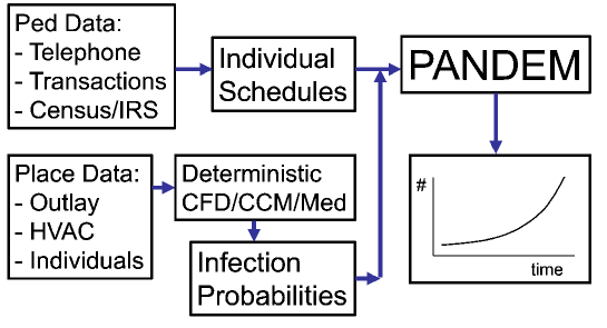
Figure 1. Global Pandemic Simulation Codes

The highest uncertainty of these types of models is the transmission rate in given settings. It is easy to see that climate (heating, cooling, ventilation), customs (hugging, kissing, proximity) and population behaviour (masking) can lead to vastly different transmission rates for the same setting (public office, classroom, meeting room, factory, airport, train station, cinema, theater, stadium, restaurant, etc.). Particularly for those pathogens that are very transmissible via the aerosol route (e.g. measles, Covid-19) the variability can be so large that the accuracy of these global pandemic simulation models can be called into question.
It is here that simulations based on high-fidelity physics of flows with aerosols together with pedestrian/crowd dynamics can be used to achieve a higher accuracy in the transmission rates, thus improving the accuracy of global simulation models.
This would no doubt entail a formidable undertaking. In principle, every venue would have to be analyzed. And this implies knowing the outlay and dimensions of the place, the heating, ventilation and air conditioning (HVAC) information, the possible external climate factors, the flow of people, etc. Given the variability of any of these factors, each one of these venues would in turn require a number of runs. However, the insight gained could be used to a) improve the airflow and ventilation so as to minimize pathogen transmission, b) modify the movement of people so as to minimize pathogen transmission, and c) increase the awareness of people frequenting these venues via visualization of pathogen movement.
On the other hand, the variability in the number of places frequented is also not infinite. Many crowded places belong to chains or franchises, and are therefore ’standardized’ in their outlay. Typical venues that fall under this category are fast-food restaurants. The flow here is predominantly from the customer/public area towards the kitchen/cooking area in order avoid odours. This implies that the placement (e.g. queuing) and movement of people are key factors that will affect transmission rates. Similar places that also have a ’standardized outlay’ are office and government buildings.
The present paper presents first steps in this direction. As stated before, an obvious necessity is the development of a reliable, accurate and scalable deterministic high-fidelity pathogen transmission model that incorporates the proper physics of flows, pedestrian motion and the ex/inhalation of pathogens.

2. Modeling Pathogen Transmission and Infection

Pathogen, or more generally, disease transmission models have a long history in both health sciences and applied mathematical modeling since the seminal work of Wells [99]. The probability of a person getting infected through the airborne route depends on

• That person’s exposure to the pathogen/virus (the dose) [22, 9] and

• The probability of getting infected given that level of exposure [84].

The first term depends on a variety of factors such as pathogens shed by infective persons, exposure time, air circulation patterns, etc. [72, 85, 100, 54, 90, 84, 30, 47, 86, 29, 29, 33, 55, 87, 73, 88, 98, 3, 4, 5, 97, 92]. In aggregate models, which include the vast majority of models, the specific locations of susceptible persons are not explicitly considered. Rather, one makes assumptions so that these locations do not have to be specified. For example, the viral particles may be assumed to be uniformly distributed, in which case the specific locations of persons are not required. More sophisticated models can account for spatial heterogeneity by dividing the space into multiple zones with different distributions of viral particles in each zone [2]. This requires knowing only the exposure times of persons in each zone, and not their specific positions. In individualized models, which are relatively rare, the specific positions of persons are required. For example, Gupta et al. [29] and Löhner et al. [71] consider specific seats in which passengers in a plane are seated and examine their exposure using Computational Fluid Dynamics (CFD) simulations.
The second term - the relationship between exposure and infection probability - can be deterministic or probabilistic [84, 29], with the latter being much more common. In a deterministic model, a person is considered infected if that person inhales more viral particles than a limit, called that person’s tolerance dose. In a probabilistic model, on the other hand, the infection probability depends on the extent of exposure. Models typically use variants of one of the following two approaches. In both approaches, infection probability is given by

$$p=1-e^{-c\cdot e_{m}}~{}~{},$$

where $c$ is a constant and $e_{m}$ the so-called exposure metric. In the Wells-Riley approach [99], the exposure is expressed in terms of an abstract ‘quantum’ of infection, whose relative values can be computed for different scenarios, and model parameters determined by fitting against empirical data. In a dose-response model, on the other hand, the exposure metric reflects the actual number of viral particles inhaled by the susceptible person, with detailed mechanisms for computing this value.

2.1. Relationship to Previous Work

Conventional models are aggregate, and do not consider the specific locations of individuals. Consequently, they cannot account for fine-scaled spatial heterogeneity. Individual models, such as [29, 70], do consider positions of individuals. However, they mostly consider situations where the positions of persons are fixed. This is inadequate for understanding risk associated when people move in a crowd. Namilae et al. [74] consider movement of people in a plane using pedestrian dynamics. However, that work does not account for movement of viral particles through the air. Instead, it considers infection risk based on contacts between persons in the crowd. Löhner al al. [70] consider movement of people in a fully coupled setting.

3. Requirements for Modeling Pathogen Propagation, Transmission and Mitigation

Taking into account all the information stated before, one can see that in order to arrive at advanced numerical models to compute with high fidelity pathogen propagation, transmission and mitigation, the following capabilities are required:

• Physical modeling of sneezing/coughing (exit velocities and temperature, number and distribution of particles, …);

• Physical modeling of aerosol propagation (flows with particles in an environment with moving pedestrians, geometric fidelity of the built environment, HVAC boundary conditions, …);

• Modeling of pedestrian motion (movement, proximity, …);

• Monitoring of pathogens exhaled and inhaled.

These in turn will enable the generation of the four essential pieces of information required:

• The generation of pathogen (e.g. viral) loads;

• The movement (advection, diffusion) of pathogen loads;

• The location and movement of pedestrians exhaling pathogens;

• The location and movement of pedestrians inhaling pathogens.

In the sequel, we will consider each one of these in turn. One should state from the outset that all of these quantities can vary greatly, so that any kind of model will have to be run repeatedly in order to obtain proper statistics.

4. Physical Modeling of Aerosol Propagation

The question often arises whether for pathogen transmission the motion of individual droplets needs to be computed. The larger droplets of diameters $O(1.0~{}mm)$ tend to fall ballistically. The smaller ones, with diameters $d<O(0.1~{}mm)$, tend to slow down immediately and adjust to the velocity of the surrounding air. Furthermore, they also evaporate quickly. If one considers the motion of a water particle with an initial velocity of $v_{i}=1~{}m/sec$ into quiescent air, and the usual values of $\rho_{p}=1000~{}kg/m^{3},\rho_{air}=1.2~{}kg/m^{3},\mu_{air}=1.85\cdot~{}10^{-5}~{}kg/m/s$, one can obtain the distance and time to rest, where ‘rest’ in this case is assumed as $v_{r}=0.01~{}v_{i}$. These values have been tabulated in Table 1. One can see that for diameters below $O(0.1~{}mm)$ the time and distance required for a particle to adjust to the velocity of the surrounding air is so low that for these aerosol particles one can neglect the air-particle interaction. Therefore, one can treat these aerosol particles via a transport equation that advects and diffuses the particle concentration in space and time.

Table 1. Distance and Time to Rest for Water Particles in Air With An Initial Velocity of 1m/sec

Diameter [mm]	distance to rest [m]	time to rest [sec]
1.00E-01	2.27E-02	1.20E-01
1.00E-02	2.79E-04	1.34E-03
1.00E-03	2.94E-06	1.40E-05

4.1. Equations Describing the Motion of the Air

As seen from the experimental evidence, the velocities of air encountered during coughing and sneezing never exceed a Mach-number of $Ma=0.1$. Therefore, the air may be assumed as a Newtonian, incompressible liquid, where buoyancy effects are modeled via the Boussinesq approximation. The equations describing the conservation of momentum, mass and energy for incompressible, Newtonian flows may be written as

$$\rho{\bf v}_{,t}+\rho{\bf v}\cdot\nabla{\bf v}+\nabla p=\nabla\cdot\mu\nabla{\bf v}+\rho{\bf g}+\beta\rho{\bf g}(T-T_{0})+{\bf s}_{v}~{}~{},$$

$$\nabla\cdot{\bf v}=0~{}~{},$$

$$\rho c_{p}T_{,t}+\rho c_{p}{\bf v}\cdot\nabla T=\nabla\cdot k\nabla T+s_{e}~{}~{}.$$

Here $\rho,{\bf v},p,\mu,{\bf g},\beta,T,T_{0},c_{p},k$ denote the density, velocity vector, pressure, viscosity, gravity vector, coefficient of thermal expansion, temperature, reference temperature, specific heat coefficient and conductivity respectively, and ${\bf s}_{v},s_{e}$ momentum and energy source terms (e.g. due to particles or external forces/heat sources). For turbulent flows both the viscosity and the conductivity are obtained either from additional equations or directly via a large eddy simulation (LES) assumption through monotonicity induced LES (MILES) [8, 24, 26, 38, 25, 39].
The pathogen concentration is given by an advection-diffusion equation of the form:

$$c_{,t}+{\bf v}\cdot\nabla c=\nabla\cdot k_{c}\nabla c+s_{c}~{}~{},$$

where $c,k_{c}$ denote the concentration (pathogens/volume) and diffusivity of the pathogen, and $s_{c}$ is the source (or sink) term (due to exhalation or inhalation). In addition, a series of additional ‘diagnostics’ equations may be required. One of them is the ‘age of air’ $\tau$ (a good measure for ventilation efficiency), given by:

$$\tau_{,t}+{\bf v}\cdot\nabla\tau=1~{}~{}.$$

4.2. Numerical Integration of the Motion of the Air

The last six decades have seen a large number of schemes that may be used to solve numerically the incompressible Navier-Stokes equations given by Eqns.(4.1.1-4.1.3). In the present case, the following design criteria were implemented:

• Spatial discretization using unstructured grids (in order to allow for arbitrary geometries and adaptive refinement);

• Spatial approximation of unknowns with simple linear finite elements (in order to have a simple input/output and code structure);

• Edge-based data structures (for reduced access to memory and indirect addressing);

• Temporal approximation using implicit integration of viscous terms and pressure (the interesting scales are the ones associated with advection);

• Temporal approximation using explicit, high-order integration of advective terms;

• Low-storage, iterative solvers for the resulting systems of equations (in order to solve large 3-D problems); and

• Steady results that are independent from the timestep chosen (in order to have confidence in convergence studies).

The resulting discretization in time is given by the following projection scheme [59, 60, 61]:

• Advective-Diffusive Prediction: ${\bf v}^{n},p^{n}\rightarrow{\bf v}^{*}$

  $${\bf s}^{\prime}=-\nabla p^{n}+\rho{\bf g}+\beta\rho{\bf g}(T^{n}-T_{0})+{\bf s}_{v}~{}~{},$$

  $$\rho{\bf v}^{i}=\rho{\bf v}^{n}+\alpha^{i}\gamma{\Delta t}\left(-\rho{\bf v}^{i-1}\cdot\nabla{\bf v}^{i-1}+\nabla\cdot\mu\nabla{\bf v}^{i-1}+{\bf s}^{\prime}\right)~{}~{};~{}~{}i=1,k-1~{}~{};$$

  $$\left[{\rho\over{\Delta t}}-\theta\nabla\cdot\mu\nabla\right]\left({\bf v}^{k}-{\bf v}^{n}\right)+\rho{\bf v}^{k-1}\cdot\nabla{\bf v}^{k-1}=\nabla\cdot\mu\nabla{\bf v}^{k-1}+{\bf s}^{\prime}~{}~{}.$$

• Pressure Correction: $p^{n}\rightarrow p^{n+1}$

  $$\nabla\cdot{\bf v}^{n+1}=0~{}~{};$$

  $$\rho{{{\bf v}^{n+1}-{\bf v}^{*}}\over{\Delta t}}+\nabla(p^{n+1}-p^{n})=0~{}~{};$$

• which results in

  $$\nabla\cdot{{\Delta t}\over\rho}\nabla(p^{n+1}-p^{n})=\nabla\cdot{\bf v}^{*}~{}~{};$$

• Velocity Correction: ${\bf v}^{*}\rightarrow{\bf v}^{n+1}$

  $${\bf v}^{n+1}={\bf v}^{*}-{{\Delta t}\over\rho}\nabla(p^{n+1}-p^{n})~{}~{}.$$

$\theta$ denotes the implicitness-factor for the viscous terms ($\theta=1$: 1st order, fully implicit, $\theta=0.5$: 2nd order, Crank-Nicholson). $\alpha^{i}$ are the standard low-storage Runge-Kutta coefficients $\alpha^{i}=1/(k+1-i)$. The $k-1$ stages of Eqn.(4.2.2) may be seen as a predictor (or replacement) of ${\bf v}^{n}$ by ${\bf v}^{k-1}$. The original right-hand side has not been modified, so that at steady-state ${\bf v}^{n}={\bf v}^{k-1}$, preserving the requirement that the steady-state be independent of the timestep ${\Delta t}$. The factor $\gamma$ denotes the local ratio of the stability limit for explicit timestepping for the viscous terms versus the timestep chosen. Given that the advective and viscous timestep limits are proportional to:

$${\Delta t}_{a}\approx{h\over{|{\bf v}|}}~{}~{};~{}~{}{\Delta t}_{v}\approx{{\rho h^{2}}\over\mu}~{}~{},$$

we immediately obtain

$$\gamma={{{\Delta t}_{v}}\over{{\Delta t}_{a}}}\approx{{\rho|{\bf v}|h}\over{\mu}}\approx Re_{h}~{}~{},$$

or, in its final form:

$$\gamma=min(1,Re_{h})~{}~{}.$$

In regions away from boundary layers, this factor is $O(1)$, implying that a high-order Runge-Kutta scheme is recovered. Conversely, for regions where $Re_{h}=O(0)$, the scheme reverts back to the usual 1-stage Crank-Nicholson scheme. Besides higher accuracy, an important benefit of explicit multistage advection schemes is the larger timestep one can employ. The increase in allowable timestep is roughly proportional to the number of stages used (and has been exploited extensively for compressible flow simulations [46]). Given that for an incompressible solver of the projection type given by Eqns.(4.2.1-4.2.7) most of the CPU time is spent solving the pressure-Poisson system Eqn.(4.2.6), the speedup achieved is also roughly proportional to the number of stages used.
At steady state, ${\bf v}^{*}={\bf v}^{n}={\bf v}^{n+1}$ and the residuals of the pressure correction vanish, implying that the result does not depend on the timestep ${\Delta t}$.
The spatial discretization of these equations is carried out via linear finite elements. The resulting matrix system is re-written as an edge-based solver, allowing the use of consistent numerical fluxes to stabilize the advection and divergence operators [61].
The energy (temperature) equation (Eqn.(4.1.3)) is integrated in a manner similar to the advective-diffusive prediction (Eqn.(4.2.2)), i.e. with an explicit, high order Runge-Kutta scheme for the advective parts and an implicit, 2nd order Crank-Nicholson scheme for the conductivity.

4.3. Immersed Body Techniques

The information required from computational crowd dynamics (CCD) codes consists of the pedestrians in the flowfield, i.e. their position, velocity, temperature, as well inhalation and exhalation. As the CCD codes describe the pedestrians as points, circles or ellipses, a way has to be found to transform this data into 3-D objects. Two possibilities have been pursued here:

• a) Transform each pedestrian into a set of (overlapping) spheres that approximate the body with maximum fidelity with the minimum amount of spheres;

• b) Transform each pedestrian into a set of tetrahedra that approximate the body with maximum fidelity with the minimum amount of tetrahedra.

The reason for choosing spheres or tetrahedra is that due to their geometric simplicity one can perform the required interpolation/ information transfer much faster than with other polyhedra or geometric shapes.
In order to ‘impose’ on the flow the presence of a pedestrian the immersed boundary methodology is used. The key idea is to prescribe at every CFD point covered by a pedestrian the velocity and temperature of the pedestrian. For the CFD code, this translates into an extra set of boundary conditions that vary in time and space as the pedestrians move. This is by now a mature technology (see, e.g. chapter 18 in [61] and the references cited therein). Fast search techniques as well as extensions to higher order boundary conditions may be found in [61, 62]. Nevertheless, as the pedestrians potentially change location at every timestep, the search for and the imposition of new boundary conditions can add a considerable amount of CPU as compared to ‘flow-only’ runs.

5. Modeling of Pedestrian Motion

The modeling of pedestrian motion has been the focus of research and development for more than two decades [23, 77, 76]. If one is only interested in average quantities (average density, velocity), continuum models [37] are an option. For problems requiring more realism, approaches that model each individual are required [91]. Among these, discrete space models (such as cellular automata [6, 7, 89, 21, 81, 49, 50, 17, 52]), force-based models (such as the social force model [34, 36, 78, 51, 63]) and agent-based techniques [75, 83, 31, 32, 94, 93, 18] have been explored extensively. Together with insights from psychology and neuroscience (e.g. [96, 93]) it has become clear that any pedestrian motion algorithm that attempts to model reality should be able to mirror the following empirically known facts and behaviours:

• Newton’s laws of motion apply to humans as well: from one instant to another, we can only move within certain bounds of acceleration, velocity and space;

• Contact between individuals occurs for high densities; these forces have to be taken into account;

• Humans have a mental map and plan on how they desire to move globally (e.g. first go here, then there, etc.);

• Human motion is therefore governed by strategic (long term, long distance), tactical (medium term, medium distance) and operational (immediate) decisions;

• In even moderately crowded situations of one person per square meter (i.e. $O(1~{}p/m^{2})$), humans have a visual horizon of $O(2.5-5.0m)$, and a perception range of 120 degrees; thus, the influence of other humans beyond these thresholds is minimal;

• Humans have a ‘personal comfort zone’; it is dependent on culture and varies from individual to individual, but it cannot be ignored;

• Humans walk comfortably at roughly 2 paces per second (frequency: $\nu=2~{}Hz$); they are able to change the frequency for short periods of time, but will return to $2~{}Hz$ whenever possible.

We remark that many of the important and groundbreaking work cited previously took place within the gaming/visualization community, where the emphasis is on ‘looking right’. Here, the aim is to answer civil engineering or safety questions such as maximum capacity, egress times under emergency, or comfort. Therefore, comparisons with experiments and actual data are seen as essential [63, 41, 42].

5.1. The PEDFLOW Model

The PEDFLOW model [63] incorporates these requirements as follows: individuals move according to Newton’s laws of motion; they follow (via will forces) ‘global movement targets’; at the local movement level, the motion also considers the presence of other individuals or obstacles via avoidance forces (also a type of will force) and, if applicable, contact forces. Newton’s laws:

$$m{{d{\bf v}}\over{dt}}={\bf f}~{}~{},~{}~{}{{d{\bf x}}\over{dt}}={\bf v}~{}~{},$$

where $m,{\bf v},{\bf x},{\bf f},t$ denote, respectively, mass, velocity, position, force and time, are integrated in time using a 2nd order explicit timestepping technique. The main modeling effort is centered on ${\bf f}$. In the present case the forces are separated into internal (or will) forces [I would like to move here or there] and external forces [I collided with another pedestrian or an obstacle]. For the sake of completeness, we briefly review the main forces used. For more information, as well as verification and validation studies, see [63, 41, 42, 101, 43, 44, 45, 67].

Will Force

Given a desired velocity ${\bf v}_{d}$ and the current velocity ${\bf v}$, this force will be of the form

$${\bf f}_{will}=g_{w}\left({\bf v}_{d}-{\bf v}\right)~{}~{}.$$

The modelling aspect is included in the function $g_{w}$, which, in the non-linear case, may itself be a function of ${\bf v}_{d}-{\bf v}$. Suppose $g_{w}$ is constant, and that only the will force is acting. Furthermore, consider a pedestrian at rest. In this case, we have:

$$m{{d{\bf v}}\over{dt}}=g_{w}\left({\bf v}_{d}-{\bf v}\right)~{}~{},~{}~{}{\bf v}(0)=0~{}~{},$$

which implies:

$${\bf v}={\bf v}_{d}\left(1-e^{-\alpha t}\right)~{}~{},~{}~{}\alpha={{g_{w}}\over{m}}={1\over t_{r}}~{}~{},$$

and

$${{d{\bf v}}\over{dt}}(t=0)=\alpha{\bf v}_{d}={{\bf v}_{d}\over t_{r}}~{}~{}.$$

One can see that the crucial parameter here is the ‘relaxation time’ $t_{r}$ which governs the initial acceleration and ‘time to desired velocity’. Typical values are ${\bf v}_{d}=1.35~{}m/sec$ and $t_{r}=O(0.5~{}sec)$. The ‘relaxation time’ $t_{r}$ is clearly dependent on the fitness of the individual, the current state of stress, desire to reach a goal, climate, signals, noise, etc. Slim, strong individuals will have low values for $t_{r}$, whereas obese or weak individuals will have high values for $t_{r}$. Furthermore, dividing by the mass of the individual allows all other forces (obstacle and pedestrian collision avoidance, contact, etc.) to be scaled by the ‘relaxation time’ as well, simplifying the modeling effort considerably.

The direction of the desired velocity

$${\bf s}={{{\bf v}_{d}}\over{|{\bf v}_{d}|}}$$

will depend on the type of pedestrian and the cases considered. A single individual will have as its goal a desired position ${\bf x}_{d}(t_{d})$ that he/she would like to reach at a certain time $t_{d}$. If there are no time constraints, $t_{d}$ is simply set to a large number. Given the current position ${\bf x}$, the direction of the velocity is given by

$${\bf s}={{{\bf x}_{d}(t_{d})-{\bf x}}\over{|{\bf x}_{d}(t_{d})-{\bf x}|}}~{}~{},$$

where ${\bf x}_{d}(t_{d})$ denotes the desired position (location, goal) of the pedestrian at the desired time of arrival $t_{d}$. For members of groups, the goal is always to stay close to the leader. Thus, ${\bf x}_{g}(t_{g})$ becomes the position of the leader. In the case of an evacuation simulation, the direction is given by the gradient of the perceived time to exit $\tau_{e}$ to the closest perceived exit:

$${\bf s}={{\nabla\tau_{e}}\over{|\nabla\tau_{e}}|}~{}~{}.$$

The magnitude of the desired velocity $|{\bf v}_{d}|$ depends on the fitness of the individual, and the motivation/urgency to reach a certain place at a certain time. Pedestrians typically stroll leisurely at $0.6-0.8~{}m/sec$, walk at $0.8-1.0~{}m/sec$, jog at $1.0-3.0~{}m/sec$, and run at $3.0-10.0~{}m/sec$.

Pedestrian Avoidance Forces

The desire to avoid collisions with other individuals is modeled by first checking if a collision will occur. If so, forces are applied in the direction normal and tangential to the intended motion. The forces are of the form:

$$f_{i}=f_{max}/(1+\rho^{p})~{}~{};~{}~{}\rho=|{\bf x}_{i}-{\bf x}_{j}|/r_{i}~{}~{},$$

where $x_{i}$, $x_{j}$ denote the positions of individuals $i,j$, $r_{i}$ the radius of individual $i$, and $f_{max}=O(4)f_{max}(will)$. Note that the forces weaken with increasing non-dimensional distance $\rho$. For years we have used $p=2$, but, obviously, this can (and probably will) be a matter of debate and speculation (perhaps a future experimental campaign will settle this issue). In the far range, the forces are mainly orthogonal to the direction of intended motion: humans tend to move slightly sideways without decelerating. In the close range, the forces are also in the direction of intended motion, in order to model the slowdown required to avoid a collision.

Wall Avoidance Forces

Any pedestrian modeling software requires a way to input geographical information such as walls, entrances, stairs, escalators, etc. In the present case, this is accomplished via a triangulation (the so-called background mesh). A distance to walls map (i.e. a function $d_{w}(x)$ is constructed using fast marching techniques on unstructured grids), and this allows to define a wall avoidance force as follows:

$${\bf f}=-f_{max}{1\over{1+({d_{w}\over r})^{p}}}\cdot\nabla d_{w}~{}~{},~{}~{}p=2$$

Note that $|\nabla d_{w}|=1$. The default for the maximum wall avoidance force is $f_{max}=O(8)f_{max}(will)$. The desire to be far/close to a wall also depends on cultural background.

Contact Forces

When contact occurs, the forces can increase markedly. Unlike will forces, contact forces are symmetric. Defining

$$\rho_{ij}=|{\bf x}_{i}-{\bf x}_{j}|/(r_{i}+r_{j})~{}~{},$$

these forces are modeled as follows:

$$\rho_{ij}<1\mathrel{\mathop{\mathchar 58\relax}}f=-[f_{max}/(1+\rho_{ij}^{p})]~{}~{};~{}~{}p=2$$

$$\rho_{ij}>1\mathrel{\mathop{\mathchar 58\relax}}f=-[2f_{max}/(1+\rho_{ij}^{p})]~{}~{};~{}~{}p=2$$

and $f_{max}=O(8)f_{max}(will)$.

Motion Inhibition

A key requirement for humans to move is the ability to put one foot in front of the other. This requires space. Given the comfortable walking frequency of $\nu=2~{}Hz$, one is able to limit the comfortable walking velocity by computing the distance to nearest neighbors and seeing which one of these is the most ‘inhibiting’.

Psychological Factors

The present pedestrian motion model also incorporates a number of psychological factors that, among the many tried over the years, have emerged as important for realistic simulations. Among these, we mention:

• Determination/Pushiness: it is an everyday experience that in crowds, some people exhibit a more polite behavior than others. This is modeled in PEDFLOW by reducing the collision avoidance forces of more determined or ‘pushier’ individuals. Defining a determination or pushiness parameter $\tilde{p}$, the avoidance forces are reduced by $(1-\tilde{p})$. Usual ranges for $\tilde{p}$ are $0.2\leq\tilde{p}\leq 0.8$.

• Comfort zone: in some cultures (northern Europeans are a good example) pedestrians want to remain at some minimum distance from contacting others. This comfort zone is an input parameter in PEDFLOW, and is added to the radii of the pedestrians when computing collisions avoidance and pre-contact forces.

• Right/Left Avoidance and Overtaking: in many western countries pedestrians tend to avoid incoming pedestrians by stepping towards their right, and overtake others on the left. However, this is not the norm everywhere, and one has to account for it.

5.2. Numerical Integration of the Motion of Pedestrians

The equations describing the position and velocity of a pedestrian may be formulated as a system of nonlinear Ordinary Differential Equations of the form:

$${{d{\bf u}_{p}}\over{dt}}={\bf r}({\bf u}_{p},{\bf x},{\bf u}_{f})~{}~{},$$

where ${\bf u}_{p}$ denote the variables of the pedestrians (positions, velocities, …) and ${\bf r}$ a right-hand-size that depends on ${\bf u}_{p}$, the position of the pedestrian (e.g. geographical obstacles) and the variables interpolated from the flow domain (e.g. smoke) ${\bf u}_{f}$. These ODEs are integrated with explicit Runge-Kutta schemes, typically of order 2.
The geographic information required, such as terrain data (inclination, soil/water, escalators, obstacles, etc.), climate data (temperature, humidity, sun/rain, visibility), signs, the location and accessibility of guidance personnel, as well as doors, entrances and emergency exits is stored in a so-called background grid consisting of triangular elements. This background grid is used to define the geometry of the problem. At every instance, a pedestrian will be located in one of the elements of the background grid. Given this ‘host element’ the geographic data, stored at the nodes of the background grid, is interpolated linearly to the pedestrian. The closest distance to a wall $\delta_{w}$ or exit(s) for any given point of the background grid evaluated via a fast ($O(N\ln(N))$) nearest neighbour/heap list technique ([61, 63]). For cases with visual or smoke impediments, the closest distance to exit(s) is recomputed every few seconds of simulation time.

5.3. Linkage to CFD Codes

The information required from CFD codes such as FEFLO [57, 58, 65] consists of the spatial distribution of temperature, smoke, other toxic or movement impairing substances in space, as well as pathogen distribution. This information is interpolated to the (topologically 2-D) background mesh at every timestep in order to calculate properly the visibility/ reachability of exits, routing possibilities, smoke, toxic substance or pathogen inhalation, and any other flowfield variable required by the pedestrians. As the tetrahedral grid used for the CFD code and the triangular background grid of the CCD code do not change in time, the interpolation coefficients need to be computed just once at the beginning of the coupled run. While the transfer of information from CFD to CCD is voluminous, it is very fast, adding an insignificant amount to the total run-times.

6. Coupling Methodology

The coupling methodology used is shown in Figure 2. The CFD code computes the flowfield, providing such information as temperature, smoke, toxic substance and pathogen concentration, and any other flow quantity that may affect the movement of pedestrians. These variables are then interpolated to the position where the pedestrians are, and are used with all other pertinent information (e.g. will-forces, targets, exits, signs, etc.) to update the position, velocity, inhalation of smoke, toxic substances or pathogens, state of exhaustion or intoxication, and any other pertinent quantity that is evaluated for the pedestrians. The position, velocity and temperature of the pedestrians, together with information such as sneezing or exhaling air, is then transferred to the CFD code and used to modify and update the boundary conditions of the flowfield, particles and pathogen concentrations in the regions where pedestrians are present.

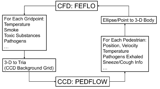
Figure 2. Coupling CFD and CCD Codes

Of the many possible coupling options (see e.g. [10, 82, 12]), we have implemented the simplest one: loose coupling with sequential timestepping ([56, 64, 68]). This is justified, as the timesteps of both the flow and pedestrian solvers are very small, so that possible coupling errors are negligible. PEDFLOW typically runs with fixed timesteps of $\Delta t_{p}=0.05~{}sec$, while the timestep chosen by FEFLO depends on mesh size and velocity. Should the timestep of FEFLO be less than the default value for PEDFLOW, then PEDFLOW automatically reduces its timestep to be the same as FEFLO. During the course of many cases run, we have never encountered any stability problems with this loose coupling and timestepping strategy.

6.1. Placement of Pathogen Loads in Space

A background grid is used for the placement of geographical information in PEDFLOW. The same grid can be used to track pathogen concentrations. As infected pedestrians move through this grid, they exhale pathogen loads - either through sneezing, coughing, shouting or talking. These pathogen loads are added to the concentration $c$ on the background grid.

6.2. Generation of Pathogen Loads

Pathogen loads are generated whenever an infected pedestrian exhales, either violently in bursts (e.g. sneezing, coughing, shouting), or continuously (e.g. loud talking). The amount of viral load can vary widely depending on the mode [72, 85, 100, 54, 90, 30, 47, 86, 33, 55, 87, 73, 88, 98, 3, 4, 5, 97, 92], the state of infection of the pedestrian, and many other factors (the term ‘superspreaders’ has been used in the medical literature). The position, velocity and orientation of pedestrians, as well as their behaviour while sneezing or coughing is transmitted from the pedestrian code to the flow code. The flow code then generates the proper boundary conditions for the exhalation. In order to simulate a sneeze/cough of duration $T_{s}$, the velocity, temperature and pathogen concentration in a spherical region of radius ($r=5~{}cm$) near the pedestrian mouth is reset at the beginning of each timestep according to the following triangular function:

$$f(t)=\begin{cases}{{2t}\over T_{s}}&if\mathrel{\mathop{\mathchar 58\relax}}0\leq t\leq T_{s}/2\cr 2-{{2t}\over T_{s}}&if\mathrel{\mathop{\mathchar 58\relax}}T_{2}/2\leq t\leq T_{s}\cr 0&if\mathrel{\mathop{\mathchar 58\relax}}T_{s}\leq t\end{cases}~{}~{},$$

$$v(t)=v_{max}f(t)~{}~{},~{}~{}T(t)=T_{a}+f(t)(T_{b}-T_{a})~{}~{},~{}~{}c(t)=c_{max}f(t)~{}~{},$$

where $T_{s}=1$ [sec], $v_{max}=O(5)$ [m/sec], $T_{a}=20$ [^oC], $T_{b}=37$ [^oC], and $c_{max}$ an estimated concentration of virons exhaled that depends on the health of the pedestrian (in the present case simply set to $c_{max}=1$ in arbitrary units). The direction of the velocity is set from the orientation of the pedestrian. The walking velocity of the pedestrian is then added in order to obtain the final value. We remark that this simplified model represents a cross-section of experimental data [16, 27, 28], but that this is an active area of research [11].

6.3. Inhalation of Pathogen Loads

As pedestrians walk or run through the clouds of viral loads, they inhale a certain amount of viruses. Given the local concentration of viral load $c$ and the breathing rate of a pedestrian, the total number of viruses inhaled can be integrated in time. The assumption is made that once the inhaled viral load reaches the infectious dose, the pedestrian is considered infected.

7. Examples

In the sequel, we show examples of different situations. We remark that these are by no means exhaustive or unique: the simulation of aerosol transmission via high-fidelity CFD techniques has received considerable attention in recent years, and has been carried out with commercial and open source software worldwide (see, e.g. [40, 95, 102, 1, 19, 20, 53, 69, 103, 70]). The CFD code used is FEFLO, which was validated for the class of problems considered here over many years [79, 80, 14, 15, 60, 66].

7.1. Fast Food Restaurant

This case considers a typical fast food restaurant. The floorplan, geometry and general outlay are shown in Figure 3. Pedestrians enter the door at a rate of 0.1 p/sec, line up in the queue, order the food that can be seen behind the counter, and then pay at the cashier. The (random) ‘loiter times’ at each of the stations along the counter with the food ranged from $t_{loit}=20-40~{}sec$.

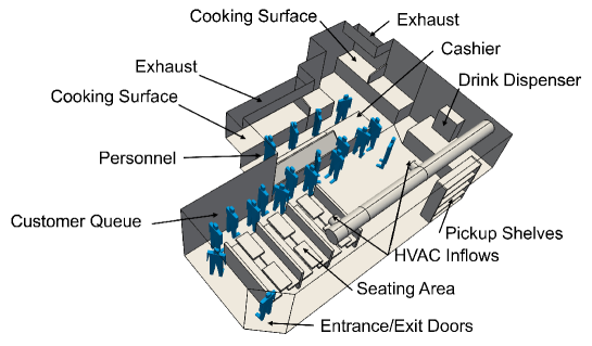
Figure 3. Fast Food Restaurant: Floorplan

The air in the room is refreshed via two HVAC inflow ducts close to the ceiling and two large exhaust surfaces located above the cooking surfaces. The initial airflow was considered at rest, and the room temperature was assumed to be $T_{0}=20^{o}C$. The air coming in from the two HVAC inflow ducts has a velocity of $v_{HVAC}=2~{}m/sec$ and a temperature of $T_{HVAC}=18^{o}C$. The heat released by the cooking surfaces was modeled via a volumetric source that occupied 20 cm above the cooking surfaces with a specific strength of $q=10^{4}~{}W/m^{3}$. At the beginning, all pedestrians are considered healthy. Thereafter, 70% of the pedestrians entering are assigned as healthy, 10% as infected but asymptomatic (i.e. not infecting) and 20% as infected and infecting. For the infecting pedestrians, the average time between sneezing is set to $\Delta t_{s}=30~{}sec$ with a variation of $\delta t_{s}=5~{}sec$ and a sneeze duration of $T_{s}=1~{}sec$. The mesh size in the region of the pedestrians was set to $h=0.05~{}m$, which implies approximately 10 flow points per pedestrian cross-section of $d_{p}=0.50~{}m$, sufficient in order to obtain the vortical motion due to pedestrian movement or flow obstruction. The total mesh size was in excess of $1.8\cdot 10^{7}$ elements. The two minutes of simulated time took approximately 48 hours using 32 cores. The results obtained are shown in Figures 4–6. Note the abscence of viral matter at the beginning. However, after approximately two minutes (during which time two sneezing events occured), a large area that is occupied by pedestrians shows the presence of viral matter, highlighting the need for better ventilation close to the entrance. The fluid dynamic explanation is that the second ventilation outlet ‘blocks’ the entrance region, producing a semi-stagnant region of recirculating flow where viral matter can build up.

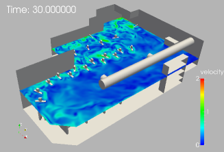
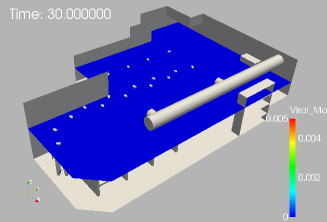
Figure 4. Fast Food Restaurant: Velocity and Viral Load at $t=30.00~{}sec$.

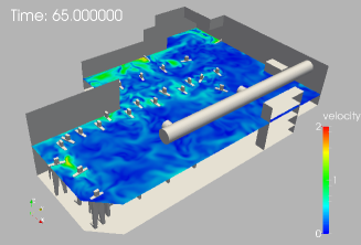
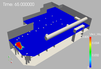
Figure 5. Fast Food Restaurant: Velocity and Viral Load at $t=65.00~{}sec$

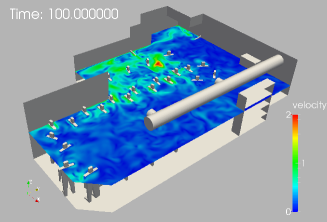
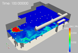
Figure 6. Fast Food Restaurant: Velocity and Viral Load at $t=100.00~{}sec$

7.2. Long Passage in Train Station

This case considers a typical rush hour scenario in a train station. The geometry and initial conditions are shown in Figure 7. The central part of the passage is 82 m long, 10 m wide and 4 m high. Several open windows are located along the passage. The inflow velocity of the windows on the right side was set to $v_{in}=1~{}m/sec$. A steady stream of pedestrians enters through both extremes and then moves towards the exit on the other side. The pedestrian flux is $2~{}p/sec$, i.e. $1~{}p/sec$ per entrance. This leads to an average number of approximately 250 pedestrians in the simulation domain at any given time during the simulaiton. At the beginning, all pedestrians are considered healthy. Thereafter, 70% of the pedestrians entering are assigned as healthy, 10% as infected but asymptomatic (i.e. not infecting) and 20% as infected and infecting. For the infecting pedestrians, the average time between sneezing is set to $\Delta t_{s}=30~{}sec$ with a variation of $\delta t_{s}=5~{}sec$ and a sneeze duration of $T_{s}=1~{}sec$. The mesh size in the region of the pedestrians was set to $h=0.0625~{}m$, which implies approximately 8 flow points per pedestrian cross-section of $d_{p}=0.50~{}m$. Not very accurate, but sufficient in order to obtain the vortical motion due to pedestrian movement. The total mesh size was in excess of $1.2\cdot 10^{8}$ elements. The two minutes of simulated time took approximately 8 hours using 1,024 cores. The results obtained are shown in Figures 8–11. Note the gradual buildup of viral matter, even though fresh air is streaming in through the windows. The simulation clearly shows the need for better ventilation: after a while, almost all pedestrians are wading through a ‘soup of viral matter’. The number of pedestrians sneezing at any given moment has been recorded in Figure 12. For a given (ableit arbitrary) threshold of $10^{-4}$ units of viral matter, the number of new infections is shown in Figure 13. The amount of viral load inhaled by the pedestrians in the simulation at time $T=120~{}sec$ may be discerned in Figure 14.

Figure 7. Long Passage: Initial Conditions

Figure 8. Long Passage: Velocity and Viral Load at $t=30.00~{}sec$

Figure 9. Long Passage: Velocity and Viral Load at $t=60.00~{}sec$

Figure 10. Long Passage: Velocity and Viral Load at $t=90.00~{}sec$

Figure 11. Long Passage: Velocity and Viral Load at $t=120.00~{}sec$

Figure 12. Long Passage: Number of Pedestrians Sneezing

Figure 13. Long Passage: Number of New Infections

Figure 14. Long Passage: Viral Load Statistics at $t=120.00~{}sec$. Blue Curve: Number of Pedestrians That Inhaled a Given Viral Load. Black Curve: Cumulative Number of Pedestrians

8. Conclusions and Outlook

A deterministic pathogen transmission model based on high-fidelity physics has been developed. The model combines computational fluid dynamics and computational crowd dynamics in order to be able to provide accurate tracing of viral matter that is exhaled, transmitted and inhaled via aerosols. The examples shown indicate that even with modest computing resources, the propagation and transmission of viral matter can be simulated for relatively large areas with thousands of square meters, hundreds of pedestrians and several minutes of physical time. The results obtained and insights gained from these simulations can be used to inform global pandemic propagation models, increasing substantially their accuracy.
As with any technology, further advances are clearly possible. The list is long, and we just mention:

• Improved knowledge of the amount of virons in the droplets exhaled by infecting individuals;

• Improved knowledge of the infectious dose required to trigger infection/illness;

• Improved boundary conditions for HVAC exits; and

• Improved modeling of particle retention and movement through cloths (e.g. for masks); and

• Improved knowledge of the effectivity of filters in HVAC systems that recirculate a percentage of the air in rooms.

Furthermore, even though the basic physical phenomena and the partial and ordinary differential equations describing them have been known for over a century, and solvers have advanced considerably over the last four decades, a vigorous experimental program is needed to complement and validate the numerical methods, and to establish firm ‘best practice’ guidelines.

References

- [1] M. Abuhegazy, K. Talaat, O. Anderoglu and S.V. Poroseva - Numerical Investigation of Aerosol Transport in a Classroom with Relevance to COVID-19; Phys. Fluids 32, 103311 (2020); https://doi.org/10.1063/5.0029118
- [2] T.W. Armstrong and C.N. Haas - A Quantitative Microbial Risk Assessment Model for Legionnaires’ Disease: Animal Model Selection and Dose-Response Modeling; Â Risk Anal. 27(6):1581-1596 (2007). https://doi.org/10.1111/j.1539-6924.2007.00990.x
- [3] S. Asadi, A.S. Wexler, C.D. Cappa, S. Barreda, N.M. Bouvier and W. Ristenpart - Aerosol Emission and Superemission During Human Speech Increase with Voice Loudness; Nature Scientific Reports 9, (1):2348 (2019). www.nature.com/scientificreports/ https://doi.org/10.1038/s41598-019-38808-z
- [4] S. Asadi, A.S. Wexler, C.D. Cappa, S. Barreda, N.M. Bouvier and W. Ristenpart - Effect of Voicing and Articulation Manner on Aerosol Particle Emission During Human Speech PLoS ONE 15(1):e0227699 (2020). https://doi.org/10.1371/journal.pone.0227699
- [5] S. Asadi, N.M. Bouvier, A.S. Wexler and W. Ristenpart - The Coronavirus Pandemic and Aerosols: Does COVID-19 Transmit via Expiratory Particles ? Aerosol Science and Technology (2020). https://doi.org/10.1080/02786826.2020.1749229
- [6] V.J. Blue and J.L. Adler - Emergent Fundamental Pedestrian Flows from Cellular Automata Microsimulation; Transportation Research Record 1644, 29-36 (1998).
- [7] V.J. Blue and J.L. Adler - Flow Capacities from Cellular Automata Modeling of Proportional Splits of Pedestrians by Direction; pp. 115-22 in Pedestrian and Evacuation Dynamics (M. Schreckenberg and S.D. Sharma eds.), Springer (2002).
- [8] J.P. Boris, F.F. Grinstein, E.S. Oran, and R.J. Kolbe - New Insights Into Large Eddy Simulation; Fluid Dynamics Research 10, 199-228 (1992).
- [9] A.F. Brouwer, M.H. Weir, M.C. Eisenberg, R. Meza and J.N.S. Eisenberg - Dose-Response Relationships for Environmentally Mediated Infectious Disease Transmission Models; PLoS Comput. Biol. 13(4): e1005481 (2017). https://doi.org/ 10.1371/journal.pcbi.1005481.
- [10] H.-J. Bungartz and M. Schäfer (eds.) Fluid-Structure Interaction, Springer Lecture Notes in Computational Science and Engineering, Springer (2006).
- [11] G. Busco, S.R. Yang, J. Seo and Y.A. Hassan - Sneezing and Asymptomatic Virus Transmission; Phys. Fluids 32, 073309 (2020) https://doi.org/10.1063/5.0019090
- [12] J.R. Cebral and R. Löhner - On the Loose Coupling of Implicit Time-Marching Codes; AIAA-05-1093 (2005).
- [13] F. Camelli and R. Löhner - Assessing Maximum Possible Damage for Contaminant Release Events; Engineering Computations 21, 7, 748-760 (2004).
- [14] F. Camelli, R. Löhner, W.C. Sandberg and R. Ramamurti - VLES Study of Ship Stack Gas Dynamics; AIAA-04-0072 (2004).
- [15] F. Camelli and R. Löhner - VLES Study of Flow and Dispersion Patterns in Heterogeneous Urban Areas; AIAA-06-1419 (2006).
- [16] C. Chao, M.P. Wan, L. Morawska, G. Johnson, R. Graham, Z. Ristovski M. Hargreaves, K. Mengersen, L. Kerrie C. Steve, Y. Li, X. Xie and S. Katoshevski - Characterization of Expiration Air Jets and Droplet Size Distributions Immediately at the Mouth Opening; J. of Aerosol Science 40, 2, 122-133 (2009).
- [17] N. Courty and S. Musse - Simulation of Large Crowds Including Gaseous Phenomena; pp.206-212 in Proc. IEEE Computer Graphics International 2005, New York, June (2005).
- [18] S. Curtis and D. Manocha - Pedestrian Simulation Using Geometric Reasoning in Velocity Space; Pedestrian and Evacuation Dynamics (U. Weidmann, U. Kirsch and M. Schreckenberg eds.), Springer, Heidelberg (2012).
- [19] T. Dbouk and D. Drikakis - On Coughing and Airborne Droplet Transmission to Humans; Phys. Fluids 32, 053310 (2020).
- [20] T. Dbouk and D. Drikakis - On Respiratory Droplets and Face Masks; Phys. Fluids 32, 063303 (2020). https://doi.org/10.1063/5.0015044
- [21] J. Dijkstra, J. Jesurun and H. Timmermans - A Multi-Agent Cellular Automata Model of Pedestrian Movement; pp. 173-180 in Pedestrian and Evacuation Dynamics (M. Schreckenberg and S.D. Sharma eds.), Springer (2002).
- [22] D.R. Franz, P.B. Jahrling, A.M. Friedlander, et al. - Clinical Recognition and Management of Patients Exposed to Biological Warfare Agents; JAMA 278:399e411 (1997).
- [23] J.J. Fruin - Pedestrian Planning and Design; Metropolitan Association of Urban Designers and Environmental Planners, New York (1971).
- [24] C. Fureby and F. Grinstein - Monotonically Integrated Large Eddy Simulation of Free Shear Flows; AIAA J. 37, 5, 544-556 (1999).
- [25] J.M. Gimenez, S.R. Idelsohn, E. Oñate and R. Löhner - A Multiscale Approach for the Numerical Simulation of Turbulent Flows with Droplets; Archives of Computational Methods in Engineering 28, 4185-4204 (2021. https://doi.org/10.1007/s11831-021-09614-6
- [26] F.F. Grinstein and C. Fureby - Recent Progress on MILES for High-Reynolds-Number Flows; J. Fluids Engineering 124, 848-861 (2002).
- [27] J.K. Gupta, C-H. Lin and Q. Chen - Flow Dynamics and Characterization of a Cough; Indoor Air 19, 517-525 (2009).
- [28] J.K. Gupta, C-H. Lin and Q. Chen - Characterizing Exhaled Airflow from Breathing and Talking; Indoor Air 20, 31-39 (2010).
- [29] J.K. Gupta, C-H. Lin and Q. Chen - Risk Assessment of Airborne Infectious Diseases in Aircraft Cabins; Indoor Air 22(5), 388-395 (2012).
- [30] J.K. Gupta, C-H. Lin and Q. Chen - Transport of Expiratory Droplets in an Aircraft Cabin; Indoor Air 21, 3-11 (2011).
- [31] S.J. Guy, J. Chhugani, C. Kim, N. Satish, M. Lin, D. Manocha and P. Dubey - ClearPath: Highly Parallel Collision Avoidance for Multi-Agent Simulation; pp. 177-187 in Proc. ACM SIGGRAPH/ Eurographics Symposium on Computer Animation (D. Fellner and S. Spencer eds), Association of Computing Machinery, New York (2009).
- [32] S.J. Guy, J. Chhugani, S. Curtis, P. Dubey, M. Lin and D. Manocha - PLEdestrians: A Least-Effort Approach to Crowd Simulation; Eurographics/ ACM SIGGRAPH Symposium on Computer Animation, Madrid, Spain (2010).
- [33] S.K. Halloran, A.S. Wexler and W.D. Ristenpart - A Comprehensive Breath Plume Model for Disease Transmission via Expiratory Aerosols; PLoS ONE 7(5):e37088 (2012). https://doi.org/10.1371/journal.pone.0037088
- [34] D. Helbing and P. Molnar - Social Force Model for Pedestrian Dynamics; Phys. Rev. E, 51:4282-4286 (1995).
- [35] D. Helbing and P. Molnar - Self-Organization Phenomena in Pedestrian Crowds; 569-577 in Self-Organization of Complex Structures: From Individual to Collective Dynamics (F. Schweitzer (Ed.), London: Gordon and Breach (1997).
- [36] D. Helbing, I.J. Farkas, P. Molnár and T. Vicsek - Simulation of Pedestrian Crowds in Normal and Evacuation Situations; pp. 21-58 in Pedestrian and Evacuation Dynamics (M. Schreckenberg and S.D. Sharma eds.), Springer (2002).
- [37] R.L. Hughes - The Flow of Human Crowds; Annual Review of Fluid Mechanics 35, 169-182 (2003).
- [38] S.R. Idelsohn, N. Nigro, A. Larreteguy, J.M. Gimenez and P. Ryshakov - A Pseudo-DNS Method for the Simulation of Incompressible Fluid Flows with Instabilities at Different Scales; Int. J. Comp. Particle Mechanics (2019). https://doi.org/10.1007/s40571-019-00264-x
- [39] S.R. Idelsohn, J.M. Gimenez, N.M. Nigro and E. Oñate - The Pseudo-Direct Numerical Simulation Method for Multi-Scale Problems in Mechanics; Comput. Meth. Appl. Mech. Engrg. 380, 113774 (2021). https://doi.org/10.1016/j.cma.2021.113774
- [40] M. Ip, J.W. Tang, D.S.C. Hui, A.L.N. Wong, M.T.V. Chan, G.M. Joynt, A.T.P. So, S.D. Hall, P.K.S. Chan and J.J.Y. Sung - Airflow and Droplet Spreading Around Oxygen Masks: A Simulation Model for Infection Control Research; AJIC 35, 10, 684-689 (2007).
- [41] M. Isenhour and R. Löhner - Verification of a Pedestrian Simulation Tool Using the NIST Recommended Test Cases; The Conference in Pedestrian and Evacuation Dynamics 2014 (PED2014), Transportation Research Procedia 2, 237-245 (2014).
- [42] M. Isenhour and R. Löhner - Verification of a Pedestrian Simulation Tool Using the NIST Stairwell Evacuation Data; The Conference in Pedestrian and Evacuation Dynamics 2014 (PED2014), Transportation Research Procedia 2, 739-744 (2014).
- [43] M. Isenhour - Simulating Occupant Response to Emergency Situations; PhD Thesis, George Mason University, Fairfax, VA (2016).
- [44] M. Isenhour and R. Löhner - Validation Data from the Evacuation of a Student Center; pp. 472-479 in Proc. Pedestrian and Evacuation Dynamics 2016 (PED 2016), (W. Song, J. Ma and L. Fu eds.), University of Science and Technology Press, Hefei, China, Oct 17-21 (2016).
- [45] M. Isenhour and R. Löhner - Pedestrian Speed on Stairs: A Mathematical Model Based on Empirical Analysis for Use in Computer Simulations; pp. 529-533 in Proc. Pedestrian and Evacuation Dynamics 2016 (PED 2016), (W. Song, J. Ma and L. Fu eds.), University of Science and Technology Press, Hefei, China, Oct 17-21 (2016).
- [46] A. Jameson, W. Schmidt and E. Turkel - Numerical Solution of the Euler Equations by Finite Volume Methods using Runge-Kutta Time-Stepping Schemes; AIAA-81-1259 (1981).
- [47] G.R. Johnson, L. Morawska, Z.D. Ristovski, M. Hargreaves, K. Mengersen, C.Y.H. Chao, M.P. Wan, Y. Li , X. Xie, D. Katoshevski, S. Corbette - Modality of Human Expired Aerosol Size Distributions J. of Aerosol Science 42, 839-851 (2011).
- [48] T. Karmakharm, P. Richmond and D.M. Romano - Agent-based Large Scale Simulation of Pedestrians With Adaptive Realistic Navigation Vector Fields; EG UK Theory and Practice of Computer Graphics 2010 (J. Collomosse and I. Grimstead eds.) (2010).
- [49] A. Kessel, H. Klüpfel, J. Wahle and M. Schreckenberg - Microscopic Simulation of Pedestrian Crowd Motion; pp. 193-202 in Pedestrian and Evacuation Dynamics (M. Schreckenberg and S.D. Sharma eds.), Springer (2002).
- [50] H.L. Klüpfel - A Cellular Automation Model for Crowd Movement and Egress Simulation; Ph.D. Dissertation: Falkutät 4, Univ. Duisburg-Essen (2003).
- [51] T.I. Lakoba, D.J. Kaup and N.M. Finkelstein - Modifications of the Helbing-Molnár-Farkas-Vicsek Social Force Model for Pedestrian Evolution; Simulation 81, 339 (2005).
- [52] P.A. Langston, R. Masling and B.N. Asmar - Crowd Dynamics Discrete Element Multi-Circle Model; Safety Science 44, 395-417 (2006).
- [53] H. Li, F.Y. Leong, G. Xu, Z. Ge, Ch.W. Kang and K.H. Lim - Dispersion of Evaporating Cough Droplets in Tropical Outdoor Environment; Phys. Fluids 32, 113301 (2020) https://doi.org/10.1063/5.0026360
- [54] W.G. Lindsley, F.M. Blachere, R.E. Thewlis, A. Vishnu, K.A. Davis, G. Cao, et al. - Measurements of Airborne Influenza Virus in Aerosol Particles from Human Coughs; PLoS ONE 5:e15100 (2010).
- [55] W.G. Lindsley, T.A. Pearce, J.B. Hudnall, K.A. Davis, S.M. Davis, M.A. Fisher, et al. - Quantity and Size Distribution of Cough-Generated Aerosol Particles Produced by Influenza Patients During and After Illness; J. Occup. Environ. Hyg. 9, 443-9. (2012).
- [56] R. Löhner, C. Yang, J. Cebral, J.D. Baum, H. Luo, D. Pelessone and C. Charman - Fluid-Structure Interaction Using a Loose Coupling Algorithm and Adaptive Unstructured Grids; AIAA-95-2259 [Invited] (1995). -
- [57] R. Löhner, Chi Yang, J. Cebral, O. Soto, F. Camelli, J.D. Baum, H. Luo, E. Mestreau, D. Sharov, R. Ramamurti, W. Sandberg and Ch. Oh - Advances in FEFLO; AIAA-01-0592 (2001).
- [58] R. Löhner, Chi Yang, J. Cebral, O. Soto, F. Camelli, J.D. Baum, H. Luo, E. Mestreau and D. Sharov - Advances in FEFLO; AIAA-02-1024 (2002).
- [59] R. Löhner - Multistage Explicit Advective Prediction for Projection-Type Incompressible Flow Solvers; J. Comp. Phys. 195, 143-152 (2004).
- [60] R. Löhner, Chi Yang, J.R. Cebral, F. Camelli, O. Soto and J. Waltz - Improving the Speed and Accuracy of Projection-Type Incompressible Flow Solvers; Comp. Meth. Appl. Mech. Eng. 195, 23-24, 3087-3109 (2006).
- [61] R. Löhner - Applied CFD Techniques, Second Edition; J. Wiley & Sons (2008).
- [62] R. Löhner, J.R. Cebral, F.F. Camelli, S. Appanaboyina, J.D. Baum, E.L. Mestreau and O. Soto - Adaptive Embedded and Immersed Unstructured Grid Techniques; Comp. Meth. Appl. Mech. Eng. 197, 2173-2197 (2008).
- [63] R. Löhner - On the Modeling of Pedestrian Motion; Appl. Math. Modelling 34, 2, 366-382 (2010).
- [64] R. Löhner - Coupling Several CFD and CSD Codes in One Application; pp. 1 - 16 in Special Edition Int. J. of Multiphysics (2011).
- [65] R. Löhner, F. Camelli, J.D. Baum, O.A. Soto and F. Togashi - Advances in FEFLO; AIAA-2013-0373 (2013).
- [66] R. Löhner, F. Camelli, J.D. Baum, F. Togashi and O. Soto - On Mesh-Particle Techniques; Comp. Part. Mech. 1, 199-209 (2014).
- [67] R. Löhner, M. Baqui, E. Haug and B. Muhamad - Real-Time Micro-Modelling of a Million Pedestrians; Engineering Computations 33, 1, 217-237 (2016).
- [68] R. Löhner and F. Camelli - Tightly Coupled Computational Fluid and Crowd Dynamics; pp. 505-509 in Proc. Pedestrian and Evacuation Dynamics 2016 (PED 2016), (W. Song, J. Ma and L. Fu eds.), University of Science and Technology Press, Hefei, China, Oct 17-21 (2016).
- [69] R. Löhner, H. Antil, S. Idelsohn and E. Oñate - Detailed Simulation of Viral Propagation in the Built Environment; Computational Mechanics 66, 1093-1107 (2020). https://doi.org/10.1007/s00466-020-01881-7
- [70] R. Löhner and H. Antil - High Fidelity Modeling of Aerosol Pathogen Propagation in Built Environments With Moving Pedestrians; Int. J. Num. Meth. Biomed. Engng. 37, 3 (2021);e3428. https://doi.org/10.1002/cnm.3428
- [71] R. Löhner, H. Antil, A. Srinivasan, S. Idelsohn and E. Oñate - High-Fidelity Simulation of Pathogen Propagation, Transmission and Mitigation in the Built Environment; Archives of Computational Methods in Engineering 28, 6, 4237-4262 (2021). https://doi.org/10.1007/s11831-021-09606-6
- [72] R.G. Loudon and R.M. Roberts - Droplet Expulsion from the Respiratory Tract; Am. Rev. Respir. Dis. 95, 3, 435-442 (1967).
- [73] D.K. Milton, M.P. Fabian, B.J. Cowling, M.L. Grantham, J.J. McDevitt - Influenza Virus Aerosols in Human Exhaled Breath: Particle Size, Culturability, and Effect of Surgical Masks; PLoS Pathog. 9:e1003205 (2013).
- [74] S. Namilae, P. Derjany, A. Mubayi, M. Scotch and A. Srinivasan - Multiscale Model for Pedestrian and Infection Dynamics During Air Travel; Physical Review E 95(5), 052320 (2017).
- [75] N. Pelechano and N.I. Badler - Modeling Crowd and Trained Leader Behavior During Building Evacuation; IEEE Computer Graphics and Applications 26 (6): 80-86 (2006).
- [76] N. Pelechano, J. Allbeck and N.I. Badler - Virtual Crowds: Methods, Simulation and Control; Morgan & Claypool, San Rafael, CA (2008).
- [77] W.M. Predtetschenski and A.I. Milinski - Personenströme in Gebäuden - Berechnungsmethoden für die Projektierung; Verlaggesellschaft Rudolf Müller, Köln-Braunsfeld (1971).
- [78] M.J. Quinn, R.A. Metoyer and K. Hunter-Zaworski - Parallel Implementation of the Social Forces Model; pp. 63-74 in Proc. 2nd Int. Conf. in Pedestrian and Evacuation Dynamics (2003).
- [79] R. Ramamurti and R. Löhner - A Parallel Implicit Incompressible Flow Solver Using Unstructured Meshes; Computers and Fluids 5, 119-132 (1996).
- [80] R. Ramamurti, W.C. Sandberg and R. Löhner - Computation of Unsteady Flow Past Deforming Geometries; Int. J. Comp. Fluid Dyn. , 83-99 (1999).
- [81] A. Schadschneider - Cellular Automaton Approach to Pedestrian Dynamics - Theory; pp. 75-86 in Pedestrian and Evacuation Dynamics (M. Schreckenberg and S.D. Sharma eds.), Springer (2002).
- [82] M. Schäfer and S. Turek (eds.) - Proc. Int. Workshop on Fluid-Structure Interaction: Theory, Numerics and Applications, Herrsching (Munich), Germany, Sept. 29 - Oct 1 (2008).
- [83] A. Sud, R. Gayle, E. Andersen, S. Guy, Ming Lin and D. Manocha - Real-time Navigation of Independent Agents Using Adaptive Roadmaps; ACM Symposium on Virtual Reality Software and Technology (2007).
- [84] G.N. Sze To and C.Y. Chao - Review and Comparison Between the Wells-Riley and Dose-Response Approaches to Risk Assessment of Infectious Respiratory Diseases; Â Indoor Air 20(1):2-16 (2010). doi:10.1111/j.1600-0668.2009.00621.x.
- [85] J.W. Tang, Y. Li, I. Eames, P.K.S. Chan and G.L. Ridgway Factors Involved in the Aerosol Transmission of Infection and Control of Ventilation in Healthcare Premises; J. of Hospital Infection 64, 100-114 (2006).
- [86] J.W. Tang, C.J. Noakes, P.V. Nielsen, I. Eames, A. Nicolle, Y. Li and G.S. Settles - Observing and Quantifying Airflows in the Infection Control of Aerosol- and Airborne-Transmitted Diseases: An Overview of Approaches; J. of Hospital Infection 77 213-222 (2011).
- [87] J.W. Tang, A.D. Nicolle, J. Pantelic, G.C. Koh, L. Wang, M. Amin, C.A. Klettner, D.K.W. Cheong, C. Sekhar and K.W. Tham - Airflow Dynamics of Coughing in Healthy Human Volunteers by Shadowgraph Imaging: An Aid to Aerosol Infection Control; PLoS ONE 7, 4: e34818 (2012). doi:10.1371/journal.pone.0034818
- [88] J.W. Tang, A.D. Nicolle, C.A. Klettner, J. Pantelic, L. Wang, A. Bin Suhaimi, A.Y.L. Tan, G.W.X. Ong, R. Su, C. Sekhar, D.K.W. Cheong and K.W. Tham - Airflow Dynamics of Human Jets: Sneezing and Breathing - Potential Sources of Infectious Aerosols; PLoS ONE 8, 4: e59970 (2013). doi:10.1371/journal.pone.0059970
- [89] K. Teknomo, Y. Takeyama and H. Inamura - Review on Microscopic Pedestrian Simulation Model; Proc. Japan Society of Civil Engineering Conf. Morioka, Japan, March (2000).
- [90] P.F.M. Teunis, N. Brienen, M.E.E. Kretzschmar - High Infectivity and Pathogenicity of Influenza A Virus Via Aerosol and Droplet Transmission; Epidemics 2, 215-222 (2010).
- [91] D. Thalmann and S.R. Musse - Crowd Simulation; Springer-Verlag, London (2007).
- [92] K. K.-W. To et al. - Temporal Profiles of Viral Load in Posterior Oropharyngeal Saliva Samples and Serum Antibody Responses During Infection by SARS-CoV-2: An Observational Cohort Study; Lancet Infect. Dis. (online) (2020). https://doi.org/10.1016/S1473-3099(20)30196-1
- [93] P.M. Torrens - Moving Agent Pedestrians Through Space and Time; Annals of the Association of American Geographers 102, 1, 35-66 (2012).
- [94] G. Vigueras, M. Lozano, J.M. Ordun and F. Grimaldo - A Comparative Study of Partitioning Methods for Crowd Simulations; Applied Soft Computing 10, 225-235 (2010).
- [95] J.M. Villafruela, I. Olmedo, M. Ruiz de Adana, C. Mendez and P.V. Nielsen - CFD Analysis of the Human Exhalation Flow Using Different Boundary Conditions and Ventilation Strategies; Building and Environment 62, 191-200 (2013).
- [96] P.M. Vishton and J. E. Cutting - Wayfinding, Displacements, and Mental Maps: Velocity Fields are Not Typically Used to Determine One’s Aimpoint; J. of Experimental Psychology 21 (5): 978-995 (1995).
- [97] World Health Organization - Transmission of SARS-CoV-2: Implications for Infection Prevention Precautions; Scientific Brief, July 9 (2020). https://www.who.int/news-room/commentaries/detail/transmission-of-sars-cov-2-implications-for-infection-prevention-precautions.
- [98] J. Wei, Y. Li - Airborne Spread of Infectious Agents in the Indoor Environment; American J. of Infection Control 44, S102-S108 (2016). http://dx.doi.org/10.1016/j.ajic.2016.06.003
- [99] W.F. Wells - Airborne Contagion and Air Hygiene. An Ecological Study of Droplet Infections; Cambridge University Press (1955).
- [100] X. Xie, Y. Li, A.T.Y. Chwang, P.L. Ho, W.H. Seto - How Far Droplets Can Move in Indoor Environments - Revisiting the wells Evaporation-Falling Curve; Indoor Air 17, 211-225 (2007). doi:10.1111/j.1600-0668.2006.00469.x
- [101] J. Zhang, D. Britto, M. Chraibi, R. Löhner, E. Haug and B. Gawenat - Qualitative Validation of PEDFLOW for Description of Unidirectional Pedestrian Dynamics; The Conference in Pedestrian and Evacuation Dynamics 2014 (PED2014), Transportation Research Procedia 2, 733-738 (2014).
- [102] Y. Zhang, G. Feng, Z. Kang, Y. Bi and Y. Cai - Numerical Simulation of Coughed Droplets in Conference Room; 10th International Symposium on Heating, Ventilation and Air Conditioning, ISHVAC2017, October, 19-22 Jinan, China (2017), Procedia Engineering 205, 302-308 (2017).
- [103] T.I. Zohdi - Modeling and Simulation of the Infection Zone from a Cough; Computational Mechanics (2020). https://doi.org/10.1007/s00466-020-01875-5