Finite-time response of dynamo mean-field effects in magnetorotational turbulence

Abstract

Accretion disc turbulence along with its effect on large-scale magnetic fields plays an important role in understanding disc evolution in general, and the launching of astrophysical jets in particular. Motivated by enabling a comprehensive sub-grid description for global long-term simulations of accretions discs, we aim to further characterize the transport coefficients emerging in local simulations of magnetorotational disc turbulence. For the current investigation, we leverage a time-dependent version of the test-field method, which is sensitive to the turbulent electromotive force (EMF) generated as a response to a set of pulsating background fields. We obtain Fourier spectra of the transport coefficients as a function of oscillation frequency. These are well approximated by a simple response function, describing a finite-time build-up of the EMF as a result of a time-variable mean magnetic field. For intermediate timescales (i.e., slightly above the orbital frequency), we observe a significant phase lag of the EMF compared to the causing field. Augmented with our previous result on a non-local closure relation in space, and incorporated into a suitable mean-field description that we briefly sketch out here, the new framework will allow to drop the restrictive assumption of scale separation.

1 Introduction

Thirty years after its ultimate discovery by Balbus & Hawley (1991), the magnetorotational instability (MRI) is practically synonymous with accretion disc turbulence and is believed to be the key to understanding the structure and evolution of discs ranging from circumplanetary, to circumstellar (including those around black-holes or neutron stars, as well as the innermost and outer reaches of protoplanetary ones), all the way to active galactic nuclei.

Enhanced transport coefficients —stemming from correlated fluctuations in the MRI turbulence— have a profound impact on disc evolution. This can happen either directly, when disc accretion is enabled by angular momentum exchange through enhanced viscosity, or indirectly via a magnetocentrifugal disc outflow. Notably, the latter scenario requires large-scale ordered poloidal fields that are either created in situ by a disc dynamo (e.g., von Rekowski et al., 2003; Stepanovs et al., 2014), or —when an inherited large-scale field is invoked— are at least affected by enhanced field dissipation as a result of eddy diffusivity. Recent attempts of incorporating sub-grid-scale physics into jet-launching simulations (e.g. Bucciantini & Del Zanna, 2013; Fendt & Gaßmann, 2018; Dyda et al., 2018; Mattia & Fendt, 2020a, b; Vourellis & Fendt, 2021) illustrate the need for comprehensive parametrizations that are ideally based on first-principles, resolved MRI simulations.

Depending on (i) the level of inherited / accumulated net-vertical magnetic flux, and (ii) the relevance of the vertical disc structure, the MRI relies to a varying degree on the presence of an intrinsic dynamo of some sort to become a self sustained mechanism for powering disc accretion (see Rincon, 2019, for an excellent review on this subject). A pronounced shortcoming of non-stratified box simulations is that they are very sensitive to the vertical aspect ratio (see Shi et al., 2016; Walker & Boldyrev, 2017).

Notably, when including vertical stratification, both local-box (going back to Brandenburg et al., 1995) and global (as recent as Dhang et al., 2020) fully non-linear MRI simulations alike robustly develop near-periodic cycles in the (horizontally / azimuthally averaged) mean magnetic field with a characteristic propagation away from the disc midplane – providing a natural explanation to sustaining the MRI via a large-scale dynamo action (e.g. Brandenburg, 2005, 2008; Blackman, 2010).

The morphology of this so-called butterfly diagram —the hallmark of the mean-field dynamo— was previously found to depend somewhat on the amount of net-vertical magnetic flux (see, e.g., Gressel & Pessah, 2015; Salvesen et al., 2016). We here nevertheless focus on the limit of negligible net-vertical magnetic flux, which in a way is the crucial test for providing a robust accretion engine from MRI turbulence. Another important issue raised pertains to the onset of convective turnover (Bodo et al., 2012; Gressel, 2013; Hirose et al., 2014), which was found to drastically affect the regularity of the magnetic-field cycles (see the discussion in Coleman et al., 2017). As with the net-vertical magnetic flux, we take a rather conservative stance and focus our investigation on the isothermal case, avoiding the complications associated with arguably more realistic thermodynamic representations.

A central question that remains unanswered is whether the dynamo wave can be reconciled with a conventional $\alpha\Omega$ dynamo (i.e., driven via the interplay of helical turbulence with differential rotation), and/or whether its dynamics are enforced by the near-exact conservation of magnetic helicity at high magnetic Reynolds number (e.g. Vishniac, 2009; Gressel, 2010; Oishi & Mac Low, 2011). While the cycle period as a function of shear rate can nicely be explained using the dispersion relation of a near-critical $\alpha\Omega$ dynamo (Gressel & Pessah, 2015), the propagation direction away from the midplane is still not well understood, possibly requiring a magnetic buoyancy contribution near the midplane (Brandenburg, 1998).

Both the spatial non-locality (see Brandenburg & Sokoloff, 2002) of the dynamo closure relation, the non-instantaneous aspects (i.e., so-called “memory effects”, e.g., Hubbard & Brandenburg, 2009), as well as their combined effect (see, e.g., Rheinhardt & Brandenburg, 2012) have been demonstrated to influence the characteristics of the dynamo cycle. Another comprehensive example of how finite-time effects can influence dynamo-generated fields has been presented by Chamandy et al. (2013a, b) in the context of galactic magnetic fields. To complement our previous investigation of the scale-dependence / non-locality of the characteristic mean-field $\alpha$ effect in MRI turbulence (Gressel & Pessah, 2015, sect. 3.4), we here investigate the potential role of finite-time effects in the mean-field closure relation.

Our paper is organized in the following manner: Section 2 briefly describes the numerical simulations and introduces the newly adopted non-instantaneous closure relation to the mean-field induction equation, as well as how it can be captured using the test-field method. We present the results obtained from a fiducial MRI shearing-box simulation in Section 3, and we discuss how these findings may be exploited in the future, in Section 4.

2 Methods

As in previous work, we solve the equations of isothermal, ideal magnetohydrodynamics (MHD) in a local shearing-box (e.g. Gressel & Ziegler, 2007) frame of reference. Lacking explicit dissipation, the purist may call this an “implicit” large-eddy simulation (iLES). For practical purposes, we will nevertheless refer to these as direct numerical simulation (DNS). For brevity, we here only briefly recapitulate the essential properties of our numerical approach, and refer the reader to sections 2.1 et seqq. of Gressel & Pessah (2015) for a more in-depth discussion, motivating our particular choices.

2.1 Brief specification of the direct simulations

We here use local Cartesian coordinates, ($x$, $y$, $z$), but refer to some tensor coefficients in cylindrical components, ($r$, $\phi$, $z$), for easier comparison with global models. Differential rotation is expressed via the parameter $q\equiv{\rm d}\ln\Omega/{\rm d}\ln r=-3/2$ for a Keplerian rotation curve, and we use the “orbital advection” scheme of Stone & Gardiner (2010) to treat the background shear flow, $\mathbf{v}_{\rm K}\equiv q\,\Omega x\,\hat{{\mathbf{y}}}$, with the benefit of a position-independent truncation error. The equations expressed in the local Eulerian velocity, $\mathbf{v}$, are

$$\frac{\partial\rho}{\partial t}+\nabla\cdot\left(\rho\mathbf{v}\right) = 0\,,$$

$$\frac{\partial\left(\rho\mathbf{v}\right)}{\partial t}+\nabla\cdot\left(\rho\mathbf{vv}+\mathrm{p}^{\star}\!-\mathbf{BB}\right) = -2\rho\ \Omega\ \hat{{\mathbf{z}}}\times\mathbf{v}\ -\rho\nabla\Phi\,,$$

$$\frac{\partial\mathbf{B}}{\partial t}-\nabla\times\left(\mathbf{v}\times\mathbf{B}\right) = 0\,,$$ (1)

with the total pressure $\mathrm{p}^{\star}\equiv\mathrm{p}+\mathbf{B}^{2}/2$, and the combined (i.e., tidal plus gravitational) effective potential

$$\Phi(x,z)=q\,\Omega^{2}x^{2}+\frac{1}{2}\Omega^{2}z^{2}\,,$$ (2)

defined in the locally co-rotating frame of reference at fixed angular frequency $\bm{\Omega}\equiv\Omega\hat{{\mathbf{z}}}$. Horizontal boundary conditions are shear-periodic (see Gressel & Ziegler, 2007, for details), and we apply standard outflow conditions in the vertical direction. We chose an intermediate box size of $L_{x}\times L_{y}\times L_{z}=H\times\pi H\times 6H$ with a linear resolution of $\simeq 32/H$ in all space dimensions – amounting to $32\times 100\times 192$ cells in the radial ($x$), azimuthal ($y$), and vertical ($z$) coordinate directions, respectively. The initial plasma parameters in the disk midplane are $\beta_{\rm p}=800$ and $\beta_{\rm p}=2.2$$\,\times 10^{5}$ for the zero-net-flux contribution, and the additional net-vertical field, respectively. As previously, we include  (i) an artificial mass diffusion term (see Gressel et al., 2011) to circumvent undue time-step constraints resulting from low-density regions in the upper disc corona, and  (ii) replenish the mass lost via outflow through the vertical domain boundary to obtain an overall steady-state disc structure.

2.2 The non-instantaneous closure relation

Adopting the well established framework of mean-field magnetohydrodynamics (Krause & Raedler, 1980), we seek a parametrization for the turbulent electromotive force, $\mbox{\boldmath{${\cal E}$}}\equiv\overline{\mathbf{v}^{\prime}\!\times\!\mathbf{B}^{\prime}}$ with fluctuating magnetic and velocity fields defined as $\mathbf{B}^{\prime}\equiv\mathbf{B}-\overline{\mathbf{B}}(z)$, and $\mathbf{v}^{\prime}\equiv\mathbf{v}-\overline{\mathbf{v}}(z)$, respectively. Here, and in the following, the overbar implies geometric averaging over horizontal slabs. This is the natural choice for the adopted box geometry and trivially satisfies the Reynolds rules required for a consistent mean-field description. By virtue of its definition, the EMF captures correlations in fluctuating velocity and magnetic field, whose non-zero mean appears as a source term on the right-hand-side of the (one-dimensional) mean-field induction equation

$$\frac{\partial\overline{\mathbf{B}}(z)}{\partial t}-\nabla\times\left(\overline{\mathbf{v}}(z)\times\overline{\mathbf{B}}(z)\right)=\nabla\!\times\!\mbox{\boldmath{${\cal E}$}}(z)\,.$$ (3)

By construction, this equation describes the long-term evolution of the (comparatively slowly changing) mean magnetic field under the effect of the underlying turbulence. To make progress over a direct simulation approach, the EMF is then typically expanded into a linear functional of the mean magnetic field and its gradients as

$$\mbox{\boldmath{${\cal E}$}}_{i}(z,t)=\alpha_{ij}(z,t)\ \overline{B}_{j}(z,t)\ -\ \eta_{ij}(z,t)\ \varepsilon_{\!jzl}\,\partial_{z}\overline{B}_{l}(z,t)\,,$$ (4)

where the indices $i,j,l$ label the coordinates $x,y$ and contraction over repeated indices is understood. Note that it is unnecessary to include the radial and azimuthal gradients in our case, which is due to the homogeneity of the turbulence in any given horizontal plane.

Under steady-state conditions, the second-rank tensors, $\alpha_{ij}(z)$ and $\eta_{ij}(z)$ become time-independent and are expected to capture the statistical properties of the chaotic flow (see Krause & Raedler, 1980). If the system at hand is sufficiently anisotropic (e.g., due to rotation) and inhomogeneous (e.g., due to vertical gravity/stratification), $\alpha_{ij}(z)$ —as well as the off-diagonal elements of $\eta_{ij}(z)$— are expected to be non-vanishing. Together, the tensors encapsulate the emergence of the mean EMF as a response to imposing an external mean magnetic field — or, in general, to the presence of a self-consistently evolving mean field. The purpose of the present paper is to elucidate a possible finite-time character of this response.

Typically, the turbulent closure coefficients are thought to connect $\mbox{\boldmath{${\cal E}$}}(z,t)$ to the mean magnetic field, $\overline{B}(z,t)$, and its curl $\varepsilon_{\!jzl}\,\partial_{z}\overline{B}_{l}(z,t)$, in a local and instantaneous fashion. However, in contrast to this instantaneous characterization of the closure relation, the power-law nature of the turbulent cascade suggests that the space-time domain of dependence of $\mbox{\boldmath{${\cal E}$}}(z,t)$ is indeed finite – implying so-called “memory effects” (Hubbard & Brandenburg, 2009), that is, a delayed (i.e., out-of-phase) response to an applied mean field. Under the assumption of statistically stationary turbulence, a simple non-instantaneous closure relation (also see Gressel & Elstner, 2020) can be formulated as a convolution integral in time of the form

$$\mbox{\boldmath{${\cal E}$}}_{i}(z,t) =\int \left[\;\hat{\alpha}_{ij}(z,t^{\prime})\,\overline{B}_{j}(z,t-t^{\prime})\right.$$ (5)

$$-\left.\hat{\eta}_{ij}(z,t^{\prime})\ \varepsilon_{\!jzl}\,\partial_{z}\overline{B}_{l}(z,t-t^{\prime})\;\right]\ {\rm d}t^{\prime}\,.$$

In the local box geometry, the integral kernels $\hat{\alpha}_{ij}(z,t^{\prime})$ and $\hat{\eta}_{ij}(z,t^{\prime})$ are functions of the vertical coordinate, $z$, only. Moreover, in its Fourier-space representation, the above relation can be expressed as a simple multiplication (see Hubbard & Brandenburg, 2009, appendix A) with the Fourier transform, $\tilde{\alpha}_{ij}$, of the kernel. That is (dropping the explicit z-dependence), we write

$$\tilde{\mbox{\boldmath{${\cal E}$}}}_{i}(\omega)=\tilde{\alpha}_{ij}(\omega)\ \tilde{\overline{B}_{\!j}}(\omega)\ -\ \tilde{\eta}_{ij}(\omega)\ {\rm i}k_{z}\,\varepsilon_{\!jzl}\,\tilde{\overline{B}_{l}}(\omega)\,,$$ (6)

attributing a spectral flavor to the mean-field coefficients. While all of these quantities are in general complex functions, we can obtain real values (of, e.g., $\mbox{\boldmath{${\cal E}$}}_{i}$) in physical space and time by adding up the contributions from positive and negative frequencies.

Complementing the result of Gressel & Pessah (2015) on non-local, scale-dependent character of the mean-field effects in magnetorotational turbulence, we here aim to obtain frequency-dependent closure coefficients, corresponding to convolution kernels in the time domain. The frequency dependence can very naturally be obtained via the test-field (TF) method (Schrinner et al., 2005, 2007) employing oscillating test fields as briefly outlined in the next section.

2.3 The spectral test-field method

The defining advantage of the TF method, compared with other methods of inference, is that it relies on analytically prescribed “test fields”, that can be chosen to span a non-degenerate basis for determining all tensor coefficients in an unambiguous manner. This differs from direct inversion methods (see, e.g., discussion in Bendre et al., 2020), that are founded on the (potentially degenerate) mean fields, $\overline{\mathbf{B}}(z,t)$, developing in the DNS. To invert equation (6), and solve for the tensorial closure coefficients, $\tilde{\alpha}_{ij}(\omega)$ and $\tilde{\eta}_{ij}(\omega)$, we apply the flavor of the method where the TFs, $\overline{\mathcal{B}}_{(\mu)}(z)$, are quadruplets of trigonometric functions (also see, e.g., Brandenburg, 2005; Sur et al., 2008; Brandenburg et al., 2008):

$$\overline{\mathcal{B}}_{(0)}=\cos(\omega t)\,\cos(k_{z}z)\,\hat{{\mathbf{x}}}\,, \quad\overline{\mathcal{B}}_{(1)}=\cos(\omega t)\,\sin(k_{z}z)\,\hat{{\mathbf{x}}}\,,$$

$$\overline{\mathcal{B}}_{(2)}=\cos(\omega t)\,\cos(k_{z}z)\,\hat{{\mathbf{y}}}\,, \quad\overline{\mathcal{B}}_{(3)}=\cos(\omega t)\,\sin(k_{z}z)\,\hat{{\mathbf{y}}}\,.$$ (7)

For the purpose of determining the time-response, we here focus on a fixed vertical scale $k_{z}=k_{z}^{\rm TF}=2\pi/L_{z}$, with $L_{z}=6$ the vertical size of the box. This makes us sensitive to the coefficients representative of the largest scales available, and we refer the interested reader to section 3.4 of Gressel & Pessah (2015) for a complementary discussion about the scale dependence (also see Rheinhardt & Brandenburg, 2012, for the general case of full spatio-temporal dependence). Having specified $k_{z}^{\rm TF}$, we moreover use eleven spectral modes $\omega=\omega^{\rm TF}=\nicefrac{{1}}{{32}},\nicefrac{{1}}{{16}},\nicefrac{{1}}{{8}},\dots,16,32\times 2\pi/P_{0}$, centered around $P_{0}=\nicefrac{{1}}{{4}}$ orbit for the temporal domain. We have arrived at this sampling interval by a combination of educated guessing and trial and error, and have found a posteriori that the relevant dynamic range appears to be covered.

In total, we are hence solving $4\!\times\!11=44$ additional induction equations, one for each of the TF fluctuations, $\mathcal{B}^{\prime}(\mathbf{r},t)$, alongside the DNS. In terms of the fluctuating velocity, $\mathbf{u}$, these are

$$\partial_{t}\mathcal{B}^{\prime}=\nabla\times\left[\;\mathbf{u}^{\prime}\!\times\!\overline{\mathcal{B}}+(\overline{\mathbf{u}}+\mathbf{v}_{\rm K})\!\times\!\mathcal{B}^{\prime}-\!\overline{\mathbf{u}^{\prime}\!\times\!\mathcal{B}^{\prime}}+\mathbf{u}^{\prime}\!\times\!\mathcal{B}^{\prime}\;\right]\,.$$ (8)

Importantly, these equations are passive in that they do not influence the evolving magnetic fields in the original DNS. Since we are dealing with MRI turbulence – driven via an underlying genuinely magnetic instability – there likely are pre-existing magnetic fluctuations, $\mathbf{B}^{\prime}_{0}$, that are statistically independent from the developing (horizontal) mean fields. Such fluctuations, if correlated with the turbulent velocity, may result in an additional EMF, namely $\mbox{\boldmath{${\cal E}$}}_{0}\equiv\overline{\mathbf{u}^{\prime}\!\times\!\mathbf{B}^{\prime}_{0}}$ – which does, however, not enter our parametrization. To obtain the coefficients, we evaluate the corresponding mean electromotive force $\mbox{\boldmath{${\cal E}$}}^{(\mu)}\equiv\overline{\mathbf{v}^{\prime}\times\mathcal{B}^{\prime}_{(\mu)}}$ for each of the quadruplets from equation (7). A formal solution to equation (6) is then obtained as

$$\left(\begin{array}[]{c}\tilde{\alpha}_{ij}(k_{z},\omega)\\[2.0pt] k_{z}\ \tilde{\beta}_{ijz}(k_{z},\omega)\end{array}\right)={\rm e}^{\rm{i}\omega t}\left(\begin{array}[]{cc}\,\cos(k_{z}z)&\sin(k_{z}z)\\[2.0pt] \!-\sin(k_{z}z)&\cos(k_{z}z)\end{array}\right)\left(\begin{array}[]{c}\mbox{\boldmath{${\cal E}$}}_{i}^{(2j\!-\!2)}\\[2.0pt] \mbox{\boldmath{${\cal E}$}}_{i}^{(2j\!-\!1)}\end{array}\right)\,,$$ (9)

where the tensors $\ \tilde{\eta}_{ij}(k_{z},\omega)\$ (i.e., wrt. the current) and $\ \tilde{\beta}_{ijz}(k_{z},\omega)\$ (i.e., wrt. the field gradients) are simply related via (see Hubbard & Brandenburg, 2009)

$$\tilde{\eta}_{ij}=\varepsilon_{jkz}\,\tilde{\beta}_{ikz}\,.$$ (10)

In order to arrive to a statistical sound basis and eliminate by-chance fluctuations, equation (9) can simply be accumulated in time as needed. This appears to be particularly relevant for slowly oscillating TFs, motivating our preference of long simulations time over grid resolution. Note that in the time-dependent case, that is, for $\omega^{\rm TF}\!\neq\!0$, complex coefficients can arise, reflecting a frequency-dependent phase shift of the resulting EMF with respect to the originating oscillating TF. In practical terms, we replace the complex factor ${\rm e}^{\rm{i}\omega t}$ in equation (9) by either $\cos(\omega t)$ or $\sin(\omega t)$, in order to project the real / imaginary parts of the coefficients, respectively. In the appendix of Gressel & Elstner (2020), we have benchmarked the implementation of the described spectral TF method, using the simple test case of helical forcing in the strictly kinematic limit.

3 Results

We present results from a single generic shearing-box simulation of the MRI in the presence of a weak (i.e., midplane $\beta_{\rm p}=2.2$$\,\times 10^{5}$) net-vertical field, with $L_{z}=\pm 3\,H$ and outflow boundary conditions and a moderate resolution of 32 grid cells per pressure scale-height. The simulation quickly reaches a steady state with a dimensionless accretion stress (i.e., Reynolds + Maxwell) of about $0.01$, and we evolve the simulation for $555$ orbits to obtain decent statistics.

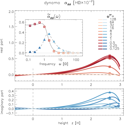
Figure 1: Profiles of the real part (upper panel /‘$\square$’) and imaginary part (lower panel / ‘$\triangle$’) of the dynamo $\alpha_{\phi\phi}(z)$ coefficient as a function of height in the disc. Each curve represents one specific value of $\omega^{\rm TF}$, and the solution sampled at $z=2.67$ is plotted in the inset as a function of angular frequency, $\omega^{\rm TF}$, of the pulsating TFs, spanning three decades in dynamic range.

In Figure 1, we plot vertical profiles of the dynamo $\alpha$ effect, where we show real (upper panel/red tones) and imaginary part (lower panel/blue tones) separately. The parametric curves represent the variation with the imposed oscillation frequency, $\omega^{\rm TF}$, of the TF inhomogeneity.

Looking at the raw array of curves by eye makes it rather cumbersome to grasp anything but the most fundamental trends in the data. As a remedy, and to illustrate the basic features of the spectral response, we resort to sampling point values at the arbitrary location $z=2.67$, roughly corresponding to the peak of the $\alpha$ profile. The real (red /‘$\square$’) and imaginary (blue /‘$\triangle$’) amplitudes thus obtained are shown in the inset of Fig. 1 along with best-fit response functions (solid/dashed, see Sect. 3.1, below, for details).

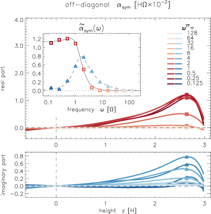
Figure 2: Same as Figure 1, but for the symmetrized off-diagonal element $\alpha_{\rm sym}\equiv\frac{1}{2}\,(\alpha_{\phi r}+\alpha_{r\phi})$ related to (differential) vertical turbulent pumping – which we note is distinct from the conventional diamagnetic pumping related to the anti-symmetrized $\gamma\equiv\frac{1}{2}\,(\alpha_{\phi r}-\alpha_{r\phi})$.

We produce a corresponding plot —shown in Fig. 2— for the symmetric off-diagonal components, $\alpha_{\rm sym}\equiv\frac{1}{2}\,(\alpha_{\phi r}+\alpha_{r\phi})$, of the dynamo tensor. One can see that apart from the overall amplitude, which is about a factor of two higher, these broadly match the characteristics of $\alpha_{\phi\phi}(z)$.

Unlike for the case of supernova-driven turbulence in the multi-phase interstellar medium (Gressel & Elstner, 2020) —where the off-diagonal elements were found to be anti-symmetric and distinct from the diagonal elements— the diagonal and off-diagonal components of the $\alpha$ tensor here (see Figs. 1 and 2, respectively) show a rather similar time response. The imaginary part displays a broad peak around $\omega=2$. At the same time, the real part has a moderate overshoot around $\omega=1$, before it reaches the asymptotic value for slowly-varying mean fields.

The general shape of the response can be understood by visualizing the overall character of (rotating) turbulence. Let us briefly recall what the $\alpha$ effect entails. It describes the emergence of a mean turbulent electromotive force as the direct consequence of the presence of a large-scale magnetic field. In the limit of high frequencies, this “presence” obviously looses its coherent character and magnetic fluctuations created by the $\mathbf{u}^{\prime}\!\times\!\overline{\mathcal{B}}$ term in Eqn. (8) will tend to become uncorrelated with the velocity and their contribution to the EMF will consequently average out to zero – this is reflected in the vanishing amplitudes towards high frequencies.

Conversely, at low frequencies, we simply approach the previously reported (Gressel & Pessah, 2015) amplitudes. In particular, the imaginary part of the effect also tends to zero in this limit, so that the $\alpha$ effect becomes a real number, implying that there is no longer a phase difference. The interesting regime falls in the region of intermediate frequencies, that roughly correspond to the eddy turnover time and/or rotational frequency of the turbulence. Here the finite-time character of the relation between the imposed large-scale field $\overline{\mathcal{B}}(t)$ (as a “cause”) and the turbulent $\mbox{\boldmath{${\cal E}$}}(t)$ (as a “response”) becomes most obvious. In particular, owing to the non-instantaneous build-up of (correlated) magnetic fluctuations via the $\mathbf{u}^{\prime}\!\times\!\overline{\mathcal{B}}$ term, the imaginary part deviates from zero, implying a phase-lag between cause and effect. Since the $\alpha$ effect is thought to be related to the twisting-up of rising field loops by the rotation (see, e.g., Rüdiger & Kitchatinov, 1993, for an analytic calculation of the expected rotational dependence), it appears natural that the effect peaks around $\omega\simeq\Omega$, where the pulsation of the assumed mean field matches the turnover of eddies that are affected by the Coriolis force.

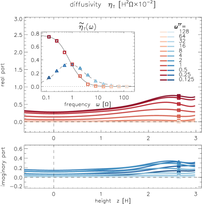
Figure 3: Same as Figure 1, but for the turbulent magnetic diffusion coefficient $\eta_{\rm T}\equiv\frac{1}{2}\,(\eta_{rr}+\eta_{\phi\phi})$ describing vertical diffusion of the field.

In comparison with the $\alpha$ tensor, the diffusion coefficient, $\eta_{\rm T}$, (shown in Figure 3) shows a somewhat reduced coherence time. This broadly matches the expectation that the mixing aspect of the chaotic flow field depends somewhat less on the buildup of correlated motions and is hence preserved further into the limit of high frequencies. Moreover, the real part of $\eta_{\rm T}(\omega)$ remains strictly monotonic around $\omega=1$, hinting at a reduced influence of the orbital timescale on the mere random diffusion of field.

3.1 Characteristic response function

Pertaining to the non-instantaneous closure relation, and for the case of simple helically-forced turbulence, Hubbard & Brandenburg (2009) have demonstrated a frequency-dependence of the form of an “oscillating decay”,

$$\alpha(t)\ \propto\ \Theta(t)\ {\rm e}^{-t/\tau_{\rm c}}\,\cos(\omega_{0}t)\,,$$ (11)

where $\Theta(t)$ simply denotes the Heaviside step function, enforcing causality by suppressing dependence on future times. Translated into Fourier space, the spectral shape function becomes

$$\tilde{\alpha}(\omega)=A_{0}\;\frac{1-{\rm i}\,\omega\,\tau_{\rm c}}{\left(1-{\rm i}\,\omega\,\tau_{\rm c}\right)^{2}+\left(\omega_{0}\,\tau_{\rm c}\right)^{2}}\,,$$ (12)

with independent coefficients $A_{0}$, $\tau_{\rm c}$, and $\omega_{0}$ – and with corresponding expressions for the other two coefficients of interest. For the purpose of curve-fitting the frequency response, we write equation (12) separated into real and imaginary part as

$$\Re = A_{0}\;\frac{1\,+\,(\omega^{2}+\omega_{0}^{2})\,\tau_{\rm c}^{2}}{4\,\omega^{2}\tau_{\rm c}^{2}+\left(1\,-\,(\omega^{2}-\omega_{0}^{2})\,\tau_{\rm c}^{2}\right)^{2}}\,,$$ (13)

$$\Im = A_{0}\;\frac{1\,+\,(\omega^{2}-\omega_{0}^{2})\,\tau_{\rm c}^{2}}{4\,\omega^{2}\tau_{\rm c}^{2}+\left(1\,-\,(\omega^{2}-\omega_{0}^{2})\,\tau_{\rm c}^{2}\right)^{2}}\;\omega\,\tau_{\rm c}\,,$$ (14)

with separate sets of fit parameters $A_{0}$, $\tau_{\rm c}$, and $\omega_{0}$ for the three coefficients $\tilde{\alpha}_{\phi\phi}(\omega)$, $\tilde{\alpha}_{\rm sym}(\omega)$, and $\tilde{\eta_{\rm T}}(\omega)$, respectively. We note that —while we express the complex dependence in terms of two separate functional shapes via equations (13) and (14)— we fit the real and imaginary branches simultaneously in practical terms.

		$A_{0}$	$\tau_{\rm c}$	$\omega_{0}$	$\omega_{0}\,\tau_{\rm c}$
dynamo	$\alpha_{\phi\phi}$	0.88	3.92	0.20	0.78
off-diagonal	$\alpha_{\rm sym}$	1.86	4.06	0.20	0.80
diffusivity	$\eta_{\rm T}$	0.56	3.05	0.17	0.52

Table 1: Fit coefficients for the complex response function defined via equations (13) and (14), along with the derived parameter $\omega_{0}\,\tau_{\rm c}\simeq 1$.

The real part (solid lines) and imaginary parts (dashed lines) of the fitted curves are overlaid in the insets of Figures 1–3, and represent the data rather well. We, moreover, report best-fit values for coefficients (sampled at $z=2.67$) in Table 1, where we also provide the dimensionless number, $\omega_{0}\tau_{\rm c}$, which we naively expect to be on the order of unity.

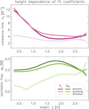
Figure 4: Height dependence of the two fit parameters from equation (12) describing the temporal behavior of the response. Circles indicate the values shown in Table 1 above. The fit amplitude, $A_{0}$, simply follows the original curves from the previous figures and is omitted here.

As a consequence of the vertical stratification in density, one may conjecture that the largest eddy–size depends on the height in the disc. This in turn should be reflected in the $\tau_{\rm c}$ and $\omega_{0}$ fit coefficients that we determine. To test this assumption, we plot the two numbers in the upper and lower panels of Figure 4, respectively. It can again be seen that the dynamo $\alpha$ term and the off-diagonal elements are very similar, and at the same time, distinct from the diffusive coefficient. While $\tau_{\rm c}$ remains fairly constant for the latter, the former two show a pronounced increase (by a factor of three) of the turbulent correlation time towards the disc midplane. In contrast to this, their oscillatory parameter, $\omega_{0}$, remains fairly even in that limit but instead shows a moderate peak around $z=1.75\,H$. As consistent with the monotonic profile seen in Fig. 3, the $\omega_{0}$ parameter is reduced in the $\eta_{\rm T}$ coefficient, and even drops to quite small values towards the disc midplane.

What precisely causes the observed trends is unclear at this point, and it is important to keep in mind that MRI turbulence is critically affected by magnetic forces so that intuition from hydrodynamic turbulence may be of limited value. Irrespective of this, comparing mean-field models with and without variation in $\tau_{\rm c}$ will allow to establish whether the seen variations do have an impact on the appearance of the butterfly diagram.

4 Discussion & Conclusions

The presented results clearly display the finite-time character of the mean-field dynamo effect emerging in stratified zero-net-flux MRI turbulence. The approximate functional form presented in the preceding section will enable to incorporate the effects into a more comprehensive mean-field description of the evolution of large-scale magnetic fields in accretion discs.

As a first step in that direction, one may neglect the $\omega_{0}$ contribution, related to oscillatory behavior at intermediate frequencies. In this case, equation (12) simplifies to

$$\tilde{\alpha}(\omega)=A_{0}^{(\alpha)}\;\frac{1}{1-{\rm i}\,\omega\,\tau_{\rm c}^{(\alpha)}}\,,$$ (15)

with corresponding expression for $\eta_{\rm T}$. With the further approximation $\tau_{\rm c}^{(\alpha)}=\tau_{\rm c}^{(\eta)}$ (cf. Table 1 for judging to what degree this is justified), the characteristic time, $\tau_{\rm c}$, enters as a relaxation time and implies a time-dependent (i.e., non-instantaneous) EMF response. In contrast to the algebraic relation from equation (4), this needs to be modeled as an extra PDE (also see Rheinhardt & Brandenburg, 2012) of the form

$$\big{(}1+\tau_{\rm c}\,\frac{\partial}{\partial t}\big{)}\;\mbox{\boldmath{${\cal E}$}}_{i}(z,t)\;=\;\alpha^{(0)}_{ij}(z)\ \overline{B}_{j}(z,t)\ -\ \eta^{(0)}_{ij}(z)\ \varepsilon_{\!jzl}\,\partial_{z}\overline{B}_{l}(z,t)\,,$$ (16)

complementing the mean-field induction equation (3), and where $\alpha^{(0)}_{ij}(z)$ and $\eta^{(0)}_{ij}(z)$ represent the above “$A_{0}$” coefficient (now measured for each tensor element individually). A very basic complete closure model would arise in combination with the non-locality derived in Gressel & Pessah (2015). Expressed as a characteristic length, $l_{\rm c}$, relating to the finite “domain of dependence”, the simplest form for the right-hand-side would then become

$$\big{(}1+\tau_{\rm c}\,\frac{\partial}{\partial t}-l_{\rm c}^{2}\frac{\partial}{\partial z^{2}}\big{)}\;\mbox{\boldmath{${\cal E}$}}_{i}(z,t)\;=\;\dots\,,$$ (17)

where the $l_{c}$ appears as a smoothing term.

This, however, still neglects the possible advection (i.e., via a term $\overline{\mathbf{u}}\cdot\nabla\,\mbox{\boldmath{${\cal E}$}}_{i}$) of the EMF with the disc outflow, $\overline{u}_{z}$, as well as potential effects related to $\nabla\cdot\overline{\mathbf{u}}=\partial_{z}\,\overline{u}_{z}$. These may act to (de-)compress the EMF – similar to the $(-\nabla\cdot\overline{\mathbf{u}})\,\overline{\mathbf{B}}$ contribution to the $\nabla\times(\overline{\mathbf{u}}\times\overline{\mathbf{B}})$ term in the induction equation itself. Moreover, if one were to restore the effect related to $\omega_{0}$, one would obtain a wave-like second-order time derivative of the EMF on the left-hand-side, as well as time derivative terms related to $\overline{\mathbf{B}}$ appearing on the right-hand side (M. Rheinhardt, private communication). A straightforward Cranck-Nicolson discretization of equation (17) has already been implemented into a simple dynamo code. In view of the mentioned complications, we however defer a detailed mean-field treatment along these lines to a later point in time.

Coming back to the inference of the dynamo coefficients from DNS, an often mentioned shortcoming of the TF method pertains to the absence of magnetic fluctuations stemming directly from the simulation. Operating in the so-called “quasi-kinematic” realm (also see discussion in Gressel & Pessah, 2015), the QK-TFM is agnostic to the presence of a possible $\mbox{\boldmath{${\cal E}$}}_{0}$, and the velocity $\mathbf{v}(\mathbf{r},t)$ is the only manifest link in equation (8) to the physical evolution traced by the DNS. While this may indeed be seen as a shortcoming of the current approach, we highlight that it merely implies that the detected mean-field effects likely are not exhaustive, but simply restricted to the chosen ansatz. A promising avenue to accounting for these additional contributions has first been laid out by Rheinhardt & Brandenburg (2010) for a simplified set of equations (i.e., lacking the pressure and self-advection terms in the momentum equation). More recently, a workable solution has been found also for the complete set of MHD equations (Käpylä, Rheinhardt & Brandenburg, 2021). It appears natural to test this approach for MRI turbulence as well.

References

- (1)
- (2)
- Balbus & Hawley (1991) Balbus S. A., Hawley J. F., 1991, ApJ, 376, 214
- Bendre et al. (2020) Bendre A. B., Subramanian K., Elstner D., Gressel O., 2020, MNRAS, 491, 3870
- Blackman (2010) Blackman E. G., 2010, AN, 331, 101
- Bodo et al. (2012) Bodo G., Cattaneo F., Mignone A., Rossi P., 2012, ApJ, 761, 116
- Brandenburg (1998) Brandenburg A., 1998, in Abramowicz M. A., Björnsson G., Pringle J. E., eds, Theory of Black Hole Accretion Disks. pp 61–90
- Brandenburg (2005) Brandenburg A., 2005, AN, 326, 787
- Brandenburg (2008) Brandenburg A., 2008, AN, 329, 725
- Brandenburg & Sokoloff (2002) Brandenburg A., Sokoloff D., 2002, GAFD, 96, 319
- Brandenburg et al. (1995) Brandenburg A., Nordlund A., Stein R. F., Torkelsson U., 1995, ApJ, 446, 741
- Brandenburg et al. (2008) Brandenburg A., Rädler K. H., Schrinner M., 2008, A&A, 482, 739
- Bucciantini & Del Zanna (2013) Bucciantini N., Del Zanna L., 2013, MNRAS, 428, 71
- Chamandy et al. (2013a) Chamandy L., Subramanian K., Shukurov A., 2013a, MNRAS, 428, 3569
- Chamandy et al. (2013b) Chamandy L., Subramanian K., Shukurov A., 2013b, MNRAS, 433, 3274
- Coleman et al. (2017) Coleman M. S. B., Yerger E., Blaes O., Salvesen G., Hirose S., 2017, MNRAS, 467, 2625
- Dhang et al. (2020) Dhang P., Bendre A., Sharma P., Subramanian K., 2020, MNRAS, 494, 4854
- Dyda et al. (2018) Dyda S., Lovelace R. V. E., Ustyugova G. V., Koldoba A. V., Wasserman I., 2018, MNRAS, 477, 127
- Fendt & Gaßmann (2018) Fendt C., Gaßmann D., 2018, ApJ, 855, 130
- Gressel (2010) Gressel O., 2010, MNRAS, 405, 41
- Gressel (2013) Gressel O., 2013, ApJ, 770, 100
- Gressel & Elstner (2020) Gressel O., Elstner D., 2020, MNRAS, 494, 1180
- Gressel & Pessah (2015) Gressel O., Pessah M. E., 2015, ApJ, 810, 59
- Gressel & Ziegler (2007) Gressel O., Ziegler U., 2007, Comp. Phys. Comm., 176, 652
- Gressel et al. (2011) Gressel O., Nelson R. P., Turner N. J., 2011, MNRAS, 415, 3291
- Hirose et al. (2014) Hirose S., Blaes O., Krolik J. H., Coleman M. S. B., Sano T., 2014, ApJ, 787, 1
- Hubbard & Brandenburg (2009) Hubbard A., Brandenburg A., 2009, ApJ, 706, 712
- Käpylä et al. (2021) Käpylä M. J., Rheinhardt M., Brandenburg A., 2021, arXiv e-prints, p. arXiv:2106.01107
- Krause & Raedler (1980) Krause F., Raedler K. H., 1980, Mean-field magnetohydrodynamics and dynamo theory
- Mattia & Fendt (2020a) Mattia G., Fendt C., 2020a, ApJ, 900, 59
- Mattia & Fendt (2020b) Mattia G., Fendt C., 2020b, ApJ, 900, 60
- Oishi & Mac Low (2011) Oishi J. S., Mac Low M.-M., 2011, ApJ, 740, 18
- Rheinhardt & Brandenburg (2010) Rheinhardt M., Brandenburg A., 2010, A&A, 520, A28
- Rheinhardt & Brandenburg (2012) Rheinhardt M., Brandenburg A., 2012, AN, 333, 71
- Rincon (2019) Rincon F., 2019, Journal of Plasma Physics, 85, 205850401
- Rüdiger & Kitchatinov (1993) Rüdiger G., Kitchatinov L. L., 1993, A&A, 269, 581
- Salvesen et al. (2016) Salvesen G., Simon J. B., Armitage P. J., Begelman M. C., 2016, MNRAS, 457, 857
- Schrinner et al. (2005) Schrinner M., Rädler K. H., Schmitt D., Rheinhardt M., Christensen U., 2005, AN, 326, 245
- Schrinner et al. (2007) Schrinner M., Rädler K.-H., Schmitt D., Rheinhardt M., Christensen U. R., 2007, GAFD, 101, 81
- Shi et al. (2016) Shi J.-M., Stone J. M., Huang C. X., 2016, MNRAS, 456, 2273
- Stepanovs et al. (2014) Stepanovs D., Fendt C., Sheikhnezami S., 2014, ApJ, 796, 29
- Stone & Gardiner (2010) Stone J. M., Gardiner T. A., 2010, ApJS, 189, 142
- Sur et al. (2008) Sur S., Brandenburg A., Subramanian K., 2008, MNRAS, 385, L15
- Vishniac (2009) Vishniac E. T., 2009, ApJ, 696, 1021
- Vourellis & Fendt (2021) Vourellis C., Fendt C., 2021, ApJ, 911, 85
- Walker & Boldyrev (2017) Walker J., Boldyrev S., 2017, MNRAS, 470, 2653
- von Rekowski et al. (2003) von Rekowski B., Brandenburg A., Dobler W., Dobler W., Shukurov A., 2003, A&A, 398, 825