Convex-roof entanglement measures of density matrices block diagonal in disjoint subspaces for the study of thermal states

Abstract

We provide a proof that entanglement of any density matrix which block diagonal in subspaces which are disjoint in terms of the Hilbert space of one of the two potentially entangled subsystems can simply be calculated as the weighted average of entanglement present within each block. This is especially useful for thermal-equilibrium states which always inherit the symmetries present in the Hamiltonian, since block-diagonal Hamiltonians are common as are interactions which involve only a single degree of freedom of a greater system. We exemplify our method on a simple Hamiltonian, showing the diversity in possible temperature-dependencies of Gibbs state entanglement which can emerge in different parameter ranges.

I Introduction

The quantification of entanglement for mixed states is a complicated problem especially once the system under study becomes larger. This is reflected in the number of entanglement measures which have been proposed and which are used to date, and the fact that no unique entanglement measure for mixed states has been established [1]. Each comes with its own set of problems, which can be broadly classified as either the need of numerical optimization of complex functions over a set of parameters which grows rapidly with system size, or the inability to detect certain types of entanglement. The first is characteristic for such measures as distillable entanglement [2, 3, 4, 5], entanglement cost [6] and all convex-roof entanglement measures, such as Entanglement of Formation (EoF) [7, 2]. Negativity [8, 9, 10] on the other hand is much easier to compute, since it only requires diagonalization, but it has no clear physical interpretation and it suffers from the second drawback, since it cannot detect bound entangled states [11, 12, 13, 14, 15, 16, 17]. Bound entangled states can occur only for systems of dimension larger than $6$ [18], so they are a small problem unless systems are relatively large, but they have been found already for very mixed states of two qutrits [11].

The quest to find efficiently computable entanglement measures that have a clear physical interpretation continues [19, 20, 21], because entanglement remains an important factor which predetermines the possibility of very quantum and nonintuitive behavior of bipartite systems. One approach is to sacrifice generality in order to obtain solvable scenarios which allows for the study of entanglement present in density matrices generated by a certain class of Hamiltonians. This has been done for qubits interacting with large environments via a Hamiltonian which leads to qubit pure decoherence [22, 23, 19] and then generalized to systems of any size [24]. The consequence here was that increased understanding of this type of entanglement allowed for schemes for its measurement to be devised [25, 26, 27], which have been experimentally tested [28].

We will be focusing on the class of convex roof entanglement measures, which are easiest to understand on an intuitive level, as they are defined by an extension of any pure-state entanglement measure to mixed states. They come with a seemingly straightforward instruction for computation, as one is to calculate the mean entanglement of the state under study decomposed into pure states and then minimize over all possible decompositions. There even exists a way to find EoF directly from the density matrix for a system of two qubits [29] and efficient minimization techniques for small bipartite systems [30]. Nevertheless, for larger systems these measures are usually not found directly using the instruction, but are evaluated on the basis of various techniques used to make minimization efficient or to bypass it entirely. These include approximations of the lower bounds of entanglement measures [31, 32, 33], direct methods for states possessing additional symmetries [34, 35, 36, 37], variational approaches to minimization and conjugate gradient methods [30, 38, 39], and the minimization over pure state extensions of the state [40]. Antother technique exchanges minimization for random sampling of possible pure-state decompositions [41, 42, 17]. The majority of the techniques benefit greatly from a reduction of the size of the Hilbert space of the system under study.

In our study we focus on a class of bipartite density matrices which are block diagonal in subspaces of the Hilbert space which are disjoint in terms of states of one of the two subsystems. We show that for such density matrices any convex-roof entanglement measure can be found as the average of the amount of entanglement contained within each block. Hence the minimization has only to be performed within the disjoint subspaces separately, substantially reducing the complexity of entanglement quantification. One consequence of this from a quantum information perspective is that bound entanglement cannot transcend between such blocks. This allows criteria which disqualify the possibility of the appearance of bound entanglement to be applied to the blocks separately, thus extending the applicability of rank and system size constraints to larger systems.

A relevant question is whether the desired structure can appear in physical systems. We mainly focus here on thermal states due to renewed interest in the context of quantum information [43, 44, 45, 46, 47]. Thermal states have the advantage that the symmetries within them are directly transferred from the Hamiltonian, thus if a Hamiltonian is block-diagonal, the corresponding thermal state will also be block diagonal within the same subspaces. The condition for the blocks to be disjoint in terms of one subsystem is commutation of the full Hamiltonian with a nontrivial operator acting solely on this part of the system. We provide examples of such Hamiltonians stemming from solid state physics. Incidentally, for this class of Hamiltonians also time evolution can retain the block diagonal structure, but this requires additional restrictions to be imposed on the initial state.

We provide exemplary dependencies of entanglement on temperature in Gibbs states for block-diagonal Hamiltonians, where the disjoint blocks are small enough to allow for the use of Wootters formula [29], while the whole system is very large. This allows us to demonstrate the efficiency of the method and study interplay of entanglement characteristics of each block within the whole state. We find that parameter changes in the Hamiltonian can lead to qualitative changes in the behavior of entanglement, some dependent on how entanglement within a given block reacts to temperature-induced mixing of the state, but most related to how the different blocks are mixed. Hence, the use of our simplified formula allows us to draw conclusions about the physics of entanglement.

The paper is organized as follows. In Sec. II we describe the class of mixed states under study and in Sec. III we briefly comment on convex-roof entanlement measures. Sec. IV contains the proof that calculation of such measures for block-diagonal density matrices of the studied type can be reduced to averaging of entanglement within separate blocks. In Sec. V we comment on the consequences of this fact from a quantum information perspective, while in Sec. VI we discuss the type of systems which will yield the desired form of the state at thermal equilibrium and during time-evolution. In Sec. VI we provide a simple example and study temperature-dependence of entanglement in different parameter ranges. Sec. VII concludes the paper.

II Entanglement in density matrices block diagonal in disjoint subspaces

We are studying bipartite density matrices and for clarity we will be calling one part the quantum system (QS) and the other part the environment (E). This is because the density matrices under consideration are asymmetric with respect to the two subsystems and an easily made distinction is necessary.

The first assumption made on the form of the joint QS-E density matrices under study is that they are block diagonal in some separable QS-E basis. Let us denote this basis as $\{|s\rangle\}$ for QS and $\{|e\rangle\}$ for E, so the density matrix is block-diagonal in basis $\{|se\rangle\equiv|s\rangle\otimes|e\rangle\}$. We will keep the notation with QS states on the left and E states on the right of the ket/tensor product throughout the paper. We further assume that the block-diagonal form is the result of the properties of E, so that each block is built of QS-E states in which the whole range QS states can be present, but the set of E states in each block is orthogonal to the states in any other block. Hence the class of density matrices under study can be written as

$$\hat{\rho}=\sum_{n}p_{n}\hat{\rho}_{n},$$ (1)

where the index $n$ distinguishes between the blocks, $p_{n}$ are probabilities with $\sum_{n}p_{n}=1$ and $\hat{\rho}_{n}$ are density matrices occupying disjoint blocks in terms of E subspaces. These density matrices not only fulfill $\hat{\rho}_{n}\hat{\rho}_{m}=0$ for $n\neq m$, but each can be written as

$$\hat{\rho}_{n}=\sum_{ss^{\prime}}\sum_{e_{n}e^{\prime}_{n}}c_{ss^{\prime}}^{ee^{\prime}}|s\rangle\langle s^{\prime}|\otimes|e_{n}\rangle\langle e^{\prime}_{n}|,$$ (2)

where all states $|e_{n}\rangle$ for a given $n$ constitute a separate subspace of E, so that $\langle e_{n}|e^{\prime}_{m}\rangle=0$ for all $e$ and $e^{\prime}$ if $n\neq m$.

Let us exemplify this on the simplest possible nontrivial density matrix, when QS is a qubit with states $|0\rangle$ and $|1\rangle$ while E is of dimension $N=4$ with states $\{|0\rangle,|1\rangle,|2\rangle,|3\rangle\}$. A mixed QS-E state

$$\hat{\rho}=\frac{1}{4}\left(|\Psi_{01}\rangle\langle\Psi_{01}|+|\Phi_{01}\rangle\langle\Phi_{01}|+|\Psi_{23}\rangle\langle\Psi_{23}|+|\Phi_{23}\rangle\langle\Phi_{23}|\right),$$ (3)

with Bell like components

$$|\Psi_{ij}\rangle = \frac{1}{\sqrt{2}}\left(|0i\rangle+|1j\rangle\right),$$ (4a)

$$|\Phi_{ij}\rangle = \frac{1}{\sqrt{2}}\left(|1i\rangle+|0j\rangle\right),$$ (4b)

can be written in matrix form as

$$\hat{\rho}=\frac{1}{8}\left(\begin{array}[]{*{8}{c}}\hfsetfillcolor{white}\hfsetbordercolor{blue}\tikzmarkin{a}(0.1,-0.1)(-0.1,0.35)\hfsetfillcolor{white}\hfsetbordercolor{red}\tikzmarkin{c}(0.1,-0.1)(-0.1,0.35)1&1&0&0&0&0&0&0\\ 1&1\tikzmarkend{c}&0&0&0&0&0&0\\ 0&0&\hfsetfillcolor{white}\hfsetbordercolor{red}\tikzmarkin{d}(0.1,-0.1)(-0.1,0.35)1&1&0&0&0&0\\ 0&0&1&1\tikzmarkend{d}\tikzmarkend{a}&0&0&0&0\\ 0&0&0&0&\hfsetfillcolor{white}\hfsetbordercolor{blue}\tikzmarkin{b}(0.1,-0.1)(-0.1,0.35)\hfsetfillcolor{white}\hfsetbordercolor{red}\tikzmarkin{e}(0.1,-0.1)(-0.1,0.35)1&1&0&0\\ 0&0&0&0&1&1\tikzmarkend{e}&0&0\\ 0&0&0&0&0&0&\hfsetfillcolor{white}\hfsetbordercolor{red}\tikzmarkin{f}(0.1,-0.1)(-0.1,0.35)1&1\\ 0&0&0&0&0&0&1&1\tikzmarkend{f}\tikzmarkend{b}\end{array}\right).$$ (5)

The QS-E basis here is separable and is arranged in the order $\{|00\rangle,|11\rangle,|01\rangle,|10\rangle,|02\rangle,|13\rangle,|03\rangle,|12\rangle\}$ to highlight the block diagonal form.

Two block structures are marked on the matrix (5). The smaller blocks (marked in red) each encompass a subspace of the Hilbert space characteristic for a single of the Bell-like states (4). These blocks do not fulfill our requirements, since the same E states can occur in different blocks, that is $\{|0\rangle,|1\rangle\}$ in the upper-left two blocks, and $\{|2\rangle,|3\rangle\}$ in the lower-right blocks. We will be studying density matrices where the block-diagonal form is of the type marked by the larger (blue) blocks, which encompass different subsets of the Hilbert space of E.

There is a fundamental difference in these two types of blocks with respect to entanglement. In the exemplary state, each smaller block encompasses a maximally entangled Bell-like state, but the mixture of two states in each larger block is separable [48], since

$$\frac{1}{2}\left(|\Psi_{ij}\rangle\langle\Psi_{ij}|+|\Phi_{ij}\rangle\langle\Phi_{ij}|\right)$$ (6)

$$=\frac{1}{2}\left(|+\rangle\langle+|\otimes|+\rangle\langle+|+|-\rangle\langle-|\otimes|-\rangle\langle-|\right),$$

with $|\pm\rangle=1/\sqrt{2}\left(|0\rangle\pm|1\rangle\right)$ on QS and $|\pm\rangle=1/\sqrt{2}\left(|i\rangle\pm|j\rangle\right)$ on E. Entanglement of the whole density matrix (5) depends on the interplay of the states contained in the small blocks, but it does not depend on the interplay of the states encompassed by the large blocks, since the separable form can be obtained in each of them separately.

As a central result of this paper, we will show that this result is general for convex-roof entanglement measures, and that the entanglement for any density matrix which is block diagonal in disjoint subspaces (1) is given by

$$E(\hat{\rho})=\sum_{n}p_{n}E(\hat{\rho}_{n}).$$ (7)

Here $E(...)$ denotes the convex-roof entanglement measure of choice.

III Convex-roof entanglement measures

We will study convex-roof entanglement measures [49, 1] for bipartite mixed state entanglement. They constitute an extension of pure-state entanglement measures to mixed states and the class of measures is defined as follows. Given a good pure state entanglement measure such as the entropy (this can be von Neumann entropy, any of the Renyi entropies, or linear entropy) of the reduced density matrix of one of the potentially entangled subsystems, $E(|\psi\rangle)$, one can construct a mixed state measure. This is done by first providing a decomposition of the density matrix into pure states,

$$\hat{\rho}=\sum_{n}P_{n}|\psi_{n}\rangle\langle\psi_{n}|,$$ (8)

where $P_{n}$ are probabilities and the states $|\psi_{n}\rangle$ do not have to be orthogonal. Note that there is an infinite number of such decompositions if the state is not pure and a full parametrization of the decompositions of a given mixed state quickly grows in complexity (and the number of free paramters) with the size of the system [50, 51, 52]. The average of pure-state entanglement

$$\tilde{E}(\hat{\rho})=\sum_{n}P_{n}E(|\psi_{n}\rangle),$$ (9)

is not enough to quantify entanglement of state (8), because the quantity (9) can strongly depend on the decomposition. Hence convex roof entanglement measures are defined as the average of pure state entanglement minimized over all possible preparations of the state (decompositions),

$$E(\hat{\rho})=\min_{\alpha}\tilde{E}(\hat{\rho}).$$ (10)

IV The proof

We prove that eq. (7) for all density matrices of the form (1) with eq. (2) fulfilled in three stages. We first study a QS composed of a single qubit and an environment with only two subspaces. In Subsection IV.2 we generalize the results to QSs of any size and finally in Subsection IV.3 we perform the simple generalization to environments with any number of subspaces.

IV.1 Qubit and environment with two subspaces

Here we study the density matrix of a qubit (the smallest possible QS) and an environment, which has two blocks with respect to E. The disjoint subspaces of E are labeled as $E_{1}$ and $E_{2}$ and their subspaces are of dimension $N_{1}$ and $N_{2}$, respectively, with $N_{1}+N_{2}=N$, where $N$ is the dimension of the whole E. The density matrix can therefore be written as

$$\hat{\rho}=p_{1}\hat{\rho}_{1}+p_{2}\hat{\rho}_{2},$$ (11)

where $p_{i}$ are probabilities with $p_{1}+p_{2}=1$ and $\hat{\rho}_{i}$ are density matrices of nontrivial dimension $2N_{i}$.

We assume that the pure state decomposition of each block that minimizes entanglement is known and we label the states by $|\phi_{i}^{k}\rangle$, where $i=1,2$ distinguishes between the blocks, so that

$$\hat{\rho}_{i}=\sum_{k}q_{i}^{k}|\phi_{i}^{k}\rangle\langle\phi_{i}^{k}|,$$ (12)

where $q_{i}^{k}$ are probabilities, with $\sum_{k}q_{i}^{k}=1$. Hence, entanglement of a given block is given by

$$E(\hat{\rho}_{i})=\sum_{k}q_{i}^{k}E(|\phi_{i}^{k}\rangle).$$ (13)

We will show that there does not exist any pure state decomposition of $\hat{\rho}$ for which entanglement is smaller than the weighed average of the entanglement present in each block, so

$$E(\hat{\rho})=p_{1}E(\hat{\rho}_{1})+p_{2}E(\hat{\rho}_{2}).$$ (14)

To this end we will first study entanglement of any pure state, here written as a superposition of states which belong to the distinct blocks

$$|\psi\rangle=\alpha|\psi_{1}\rangle+\beta|\psi_{2}\rangle.$$ (15)

These states can in turn be written as

$$|\psi_{i}\rangle=x_{i}|0\rangle\otimes|\varphi_{i}^{0}\rangle+y_{i}|1\rangle\otimes|\varphi_{i}^{1}\rangle.$$ (16)

Environmental states $|\varphi_{i}^{0}\rangle$ and $|\varphi_{i}^{1}\rangle$ do not have to be orthogonal when they belong to the same block, $\langle\varphi_{i}^{0}|\varphi_{i}^{1}\rangle\neq 0$, $i=1,2$, but they must be mutually orthogonal when they belong to different blocks, $\langle\varphi_{1}^{a}|\varphi_{2}^{b}\rangle=0$, $a,b=0,1$.

Hence, if we rewrite the state (15) in a form which simplifies the calculation of the reduced density matrix with respect to the qubit,

$$|\psi\rangle=a|0\rangle\otimes|\psi_{a}\rangle+b|1\rangle\otimes|\psi_{b}\rangle,$$ (17)

the parameters are given by

$$a = \sqrt{|\alpha|^{2}|x_{1}|^{2}+|\beta|^{2}|x_{2}|^{2}},$$ (18a)

$$b = \sqrt{|\alpha|^{2}|y_{1}|^{2}+|\beta|^{2}|y_{2}|^{2}},$$ (18b)

while the normalized environmental states are

$$|\psi_{a}\rangle = \frac{1}{a}\left(\alpha x_{1}|\varphi_{1}^{0}\rangle+\beta x_{2}|\varphi_{2}^{0}\rangle\right),$$ (19a)

$$|\psi_{a}\rangle = \frac{1}{b}\left(\alpha y_{1}|\varphi_{1}^{1}\rangle+\beta y_{2}|\varphi_{2}^{1}\rangle\right).$$ (19b)

The reduced density matrix of E is then given by

$$\hat{\rho}_{E}=a^{2}|\psi_{a}\rangle\langle\psi_{a}|+b^{2}|\psi_{b}\rangle\langle\psi_{b}|,$$ (20)

and the normalized linear entropy of the reduced density matrix, which we will use as our pure state entanglement measure, is given by

$$E(|\psi\rangle)=2\left(1-\hbox{Tr}\hat{\rho}_{E}^{2}\right)=4a^{2}b^{2}\left(1-\left|\langle\psi_{a}|\psi_{b}\rangle\right|^{2}\right).$$ (21)

Since the states of E from different subspaces have to be orthogonal to each other, we obtain a simplified formula for the scalar product

$$\left|\langle\psi_{a}|\psi_{b}\rangle\right|^{2}=\frac{1}{a^{2}b^{2}}\left||\alpha|^{2}x_{1}^{*}y_{1}\langle\varphi_{1}^{0}|\varphi_{1}^{1}\rangle+|\beta|^{2}x_{2}^{*}y_{2}\langle\varphi_{2}^{0}|\varphi_{2}^{1}\rangle\right|^{2}.$$ (22)

We will now compare the result with the average of the (normalized) linear entropy of the block diagonal density matrix

$$\hat{\rho}_{BD}=|\alpha|^{2}|\psi_{1}\rangle\langle\psi_{1}|+|\beta|^{2}|\psi_{2}\rangle\langle\psi_{2}|;$$ (23)

the matrix is a counterpart to the pure state (15), but without the inter-block coherences. This is given by (the “tilde” signifies that this quantity is not in fact an entanglement measure, since it has not been minimized)

$$\tilde{E}(\hat{\rho}_{BD})=|\alpha|^{2}E(|\psi_{1}\rangle)+|\beta|^{2}E(|\psi_{2}\rangle),$$ (24)

with

$$E(|\psi_{i}\rangle)=4|x_{i}|^{2}|y_{i}|^{2}\left(1-\left|\langle\varphi_{i}^{0}|\varphi_{i}^{1}\rangle\right|^{2}\right).$$ (25)

The difference between the pure state entanglement given by eq. (21) and the average (24) is given by

$$E(|\psi\rangle)-\tilde{E}(\hat{\rho}_{BD}) = 4|\alpha|^{2}|\beta|^{2}\left[\left(|x_{1}|^{2}-|x_{2}|^{2}\right)^{2}\right.$$

$$+\left.\left|x_{1}^{*}y_{1}\langle\varphi_{1}^{0}|\varphi_{1}^{1}\rangle-x_{2}^{*}y_{2}\langle\varphi_{2}^{0}|\varphi_{2}^{1}\rangle\right|^{2}\right]\geq 0.$$

This quantity is obviously always greater or equal to zero which means that the entanglement present in a superposition of states from the different blocks is always greater than the average of the entanglement contained in each block separately. Note that this result is only true because the different blocks are disjoint in terms of the states of E.

Given the result (IV.1) it is now straightforward to show that entanglement present in a density matrix of the form (11) is found using eq. (14). Let us start with an arbitrary pure state decomposition of $\hat{\rho}$, eq. (8), which we henceforth label with the index $A$. If we rewrite each state $|\psi_{n}\rangle$ as a superposition of states which belong to the distinct blocks as in eq. (15) with coefficients $\alpha_{n}$ and $\beta_{n}$, we get

$$\hat{\rho} = \sum_{n}P_{n}|\alpha_{n}|^{2}|\psi_{1n}\rangle\langle\psi_{1n}|+\sum_{n}P_{n}|\beta_{n}|^{2}|\psi_{2n}\rangle\langle\psi_{2n}|$$

$$+\sum_{n}P_{n}\alpha_{n}\beta_{n}^{*}|\psi_{1n}\rangle\langle\psi_{2n}|+\sum_{n}P_{n}\alpha_{n}^{*}\beta_{n}|\psi_{2n}\rangle\langle\psi_{1n}|.$$

Since the density matrix $\hat{\rho}$ is block diagonal with respect to the different subspaces, the last two terms must be equal to zero, so

$$\hat{\rho}=\hat{\rho}_{B}=\sum_{n}P_{n}|\alpha_{n}|^{2}|\psi_{1n}\rangle\langle\psi_{1n}|+\sum_{n}P_{n}|\beta_{n}|^{2}|\psi_{2n}\rangle\langle\psi_{2n}|$$ (28)

is a different pure state decomposition of the same density matrix, we label this decomposition by $B$. The crucial difference between the two decompositions is that the latter does not contain any states which encompass both subspaces, so we can write the density matrix directly in the form given by eq. (11) with individual decompositions,

$$\hat{\rho}_{i}=\frac{1}{p_{i}}\sum_{n}q_{n}^{i}|\psi_{in}\rangle\langle\psi_{in}|,$$ (29)

with $q_{n}^{1}=P_{n}|\alpha_{n}|^{2}$, $q_{n}^{2}=P_{n}|\beta_{n}|^{2}$, and $p_{i}=\sum_{n}q_{n}^{i}$. These are not necessarily the decompositions which minimize entanglement in each block separately (12).

Using the property (IV.1), we can show that the average of the (normalized) linear entropy for decomposition $A$ is always greater or equal to the average for decomposition $B$, since

$$\tilde{E}(\hat{\rho}_{A}) = \sum_{n}P_{n}E(|\psi_{n}\rangle)$$

$$\geq \sum_{n}P_{n}|\alpha_{n}|^{2}E(|\psi_{1n}\rangle)+\sum_{n}P_{n}|\beta_{n}|^{2}E(|\psi_{2n}\rangle)$$

$$= \tilde{E}(\hat{\rho}_{B}).$$

Hence, for every pure state decomposition of the block diagonal density matrix $\hat{\rho}$, there exists a decomposition which does not contain superposition states between the two subspaces of E, for which the average of pure-state entanglement is lesser or equal. The direct consequence of this is that minimization of average entanglement over all possible pure state decompositions will yield the average of entanglement minimized in each block separately, and mixed state entanglement is given by eq. (14).

IV.2 Larger quantum system

The generalization of the result of the previous section to a larger QS is rather straightforward. The first step is to show that pure state entanglement is always larger than the average entanglement of the counterpart block-diagonal density matrix, meaning that the inequality

$$E(|\psi\rangle)-\tilde{E}(\hat{\rho}_{BD})\geq 0$$ (31)

still holds. Since we are still studying the situation with two subspaces, the relevant states are given by eqs (15) and (23), with the average linear entropy of state $\hat{\rho}_{BD}$ definedy by eq. (24). We show that the inequality holds in Appendix A.

Once this is established, we can show that for any decomposition ($A$) of the density matrix (8) there exists a counter decomposition ($B$) which only contains states limited to either block, for which the average pure-state entanglement is smaller or equal. This is shown as in the previous section, by writing each state in decomposition $A$ as in eq. (15) to obtain eq. (IV.1), and then by noting that the off-diagonal terms that connect the two subspaces must sum to zero, to obtain decomposition $B$, given by eq. (28). As the averaged entanglement in the two decompositions can, as previously, be connected using the pure-state inequality (31) yielding $\tilde{E}(\hat{\rho}_{A})\geq\tilde{E}(\hat{\rho}_{B})$, it follows that any convex-roof entanglement measure of a density matrix which is block diagonal in two blocks which span different environmental subspaces is given by the average entanglement contained in each block (14) regardless of QS size.

IV.3 More subspaces

The generalization to more subspaces is even more straightforward. Obviously, since entanglement can be found by averaging the entanglement between two subspaces, if there are $M$ block diagonal subspaces in terms of E states, the entanglement of the whole density matrix can be found by averaging entanglement between one subspace and the remaining $M-1$, while the entanglement of the $M-1$ blocks can be found by averaging between one of them and the remaining $M-2$, and so on. Consequently the entanglement in a matrix of $M$ blocks can be found by averaging over the entanglement of each block, and hence is given by eq. (10).

V Consequences

In this section we discuss the consequences of the central result of this paper, namely that any convex-roof entanglement measure can be calculated using eq. (7) for density matrices which are block diagonal in disjoint subspaces, for the theory of mixed state entanglement. Outside the obvious simplification of calculation of such entanglement measures, since now minimization has to be performed separately over parts of the QS-E Hilbert space, there are two significant implications.

The first pertains to bound entanglement. Negativity [8, 9, 10]), the only measure to quantify mixed state entanglement for larger systems which can be found directly from the density matrix, is defined as the absolute sum of the negative eigenvalues of the density matrix after partial transposition with respect of one of the subsystems is performed. In other words, it is a measure based on the Peres-Horodecki criterion [53, 54], which states that if the matrix after partial transposition is not a density matrix (has negative eigenvalues) then there is entanglement in the state. The drawback of the measure and the criterion is that they do not detect certain entangled states; such states are said to contain bound entanglement [11, 12]. The existence of bound entanglement and its experimental demonstration have received a lot of attention [13, 14, 15, 16, 17], but the exact limitations on when bound entanglement can be expected are not known with the exception of small systems and states with additional symmetries.

For density matrices which are block diagonal with respect to disjoint subspaces of E, Negativity can obviously be found in each block separately, since partial transposition of the density matrix with respect to E does not mix the blocks and both the partial transposition and the calculation of eigenstates can be done in each block separately. The question remains, if there exist bound entangled states that transgress these blocks. Since we have shown that this property translates to all convex-roof entanglement measures, we have automatically shown that bound entanglement cannot exist between separate blocks of this type. It can only exist within a single block, hence imposing a new limitation on states where we can expect this type of quantum correlations.

Practically this extends the set of states for which bound entanglement is impossible to systems of any size as long as individual disjoint blocks are not greater than $6\times 6$ matrices. Less trivially, it also pushes the boundary for the rank of the studied bipartite state of dimension $M\times N$ required for bound entanglement [55, 18], since each block can be treated separately. Hence if the dimension of QS is $M$, while E is separated into $n$ disjoint blocks each of dimension $N_{i}$, with $N=\sum_{i}N_{i}$, then the general criterion that guarantees only free entanglement (not bound), namely that the rank of the density matrix has to be $\leq\max\left(M,N\right)$ is supplemented by criteria for each block, which are easier to check because of the smaller size of the blocks. For bound entanglement to be impossible in a given block, its rank must be $\leq\max\left(M,N_{i}\right)$. Note that the block criteria do not always directly imply the criterion for the full density matrix, since the dimension of a given block of the environment can be smaller than the dimension of QS.

The second implication pertains to the existence of bipartite mixed states which are classified by convex-roof entanglement measures as containing maximum entanglement. Such states were considered unlikely by the original paper on the topic [56], but states of required form were found in Ref. [57]. It has later been shown that the periodical emergence of such states is possible in qubit-environment evolutions driven by Hamiltonians that lead to pure dephasing of the qubit [19] and are important for the emergence of objectivity [58, 59, 60, 61, 62, 63, 64]. Here we have found that the emergence of such states is not limited to pure-dephasing evolutions and that they can manifest themselves in other classes of interactions.

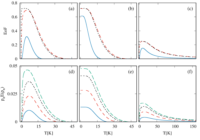
Figure 1: Entanglement at thermal equilibrium as a function of temperature for Hamiltonian formed from blocks given by eq. (32). Top panels show Entanglement of Formation for (a) finite eigenenergies $E_{m}$ and non-zero magnetic field, $\Omega=1$, (b) finite eigenenergies $E_{m}$ and zero magnetic field, $\Omega=0$, (c) infinite eigenenergies $E_{m}=\infty$ and non-zero magnetic field, $\Omega=1$. The three curves correspond to different sizes of the environment: $K=1$ - solid blue line, $K=10$ - dashed red line, $K=100$ - dotted black line. Bottom panels show corresponding [$(a)\rightarrow(d)$, etc.] components of entanglement for different blocks, $p_{n}E(\rho_{n})$ for $K=10$ with $m=-10$ - solid blue line, $m=-8$ - dashed red line , $m=-5$ - dotted black line, $m=0$ - dashed green line.

VI Relevance

The relevance of the presented proof is based on the answer to the question, if there exist physical QS-E states which have the form (1). The answer is yes and we will discuss some situations when this is the case with special focus on thermal QS-E states. In fact the requirement for a density matrix describing a state at thermal equilibrium corresponding to temperature $T$, $\hat{\rho}_{T}=\exp(-\beta\hat{H})/Z$, with $\beta=1/k_{B}T$ and $Z$ being the partition function, is that the Hamiltonian has the required form.

We will be taking into account the standard form of a Hamiltonian describing two interacting systems, so $\hat{H}=\hat{H}_{\mathrm{QS}}+\hat{H}_{\mathrm{E}}+\hat{H}_{\mathrm{QS-E}}$, where the first term describes the free Hamiltonian of QS, the second of E, and the third term describes their interaction. We require the full Hamiltonian to be block diagonal in terms of the states of E. The form of the QS part is therefore arbitrary, yet the interplay of the interaction and free Hamiltonian of E is cruitial.

There is a plethora of systems (which would here constitute E) for which the Hamiltonian commutes with at least one non-trivial observable $\hat{A}$, $[\hat{H}_{E},\hat{A}]=0$. In nontrivial situations (when the eigenstates of the observable $\hat{A}$ are degenerate in the full Hilbert space of $\hat{H}_{E}$, or, physically speaking, the observable describes only one degree of freedom, such as spin, of a more complex system) this yields a Hamiltonian which is block-diagonal in subspaces corresponding to a single eigenvalue of $\hat{A}$.

A good example here is the Hubbard model [65, 66, 67, 68, 69] as it commutes with three different operators, each reducing the dimension of the blocks. Firstly, the Hubbard Hamiltonian commutes with the number operator, meaning that each subspace of the Hilbert space where the states describe an equal number of particles constitutes a separate block. Furthermore, the Hamiltonian commutes with the total spin $\hat{S}_{z}$ component, so within each block there is a smaller block-diagonal structure, which differentiates between states with different spin symmetry. Finally, it also commutes with the parity operator, yielding even smaller non-trivial blocks. Such symmetries are common in many-body systems and are seen in e. g.  the Heisenberg, Bose-Hubbard, t-J, or Holstain models [70, 65, 71, 72, 73].

Obviously, the block-diagonal form of $\hat{H}_{E}$ is not sufficient for the full Hamiltonian to demonstrate block-diagonality with respect to environmental subspaces. To this end the interaction term must possess the same symmetries as those that yield the structure of $\hat{H}_{E}$. Namely if the Hamiltonian of E commutes with the observable $\hat{A}$, then also the interaction term must commute with it, $[\hat{H}_{int},\hat{A}]=0$. This means that during the interaction the quantum system would be susceptible to the effect of the environment with respect to some degree of freedom while another (described by the observable $\hat{A}$) would not affect it.

If the Hamiltonian has the specific block-diagonal structure not only thermal equilibrium states will retain it, but it will be kept during time-evolution as long as the initial QS-E state is a mixture of states contained within single blocks. The most natural situation when this is obtained is when the initial QS-E state is of product form with the initial E state being a thermal equilibrium state of block-diagonal $\hat{H}_{E}$. There are then no limitations on the initial states of QS.

The initial QS-E state can also be used to guarantee that the block-diagonal form of the full density matrix with disjoint subspaces is kept throughout an evolution governed by a Hamiltonian where the subspaces of the blocks partially overlap. An example of such a (full) Hamiltonian is one describing a spin interacting with an environment of spins via the hyperfine interaction in the “box model” approximation [74, 75, 76, 77]. Such a Hamiltonian is block-diagonal with disjoint subspaces with respect to the total spin operator of E, but the block-diagonality which is present in subspaces governed by the projection of the total spin operator overlap. By choosing an initial environmental state which is a mixture of states contained within these smaller subspaces, but skipping some spin quantum numbers, one could guarantee that the QS-E density matrix would have the required form throughout the evolution.

VII Examples

As an example we will study a Hamiltonian describing a qubit interacting with an environment, where the Hamiltonian is block-diagonal in terms of $4\times 4$ blocks, where each block is composed of the same $|\!\uparrow\rangle,|\!\downarrow\rangle$ qubit states and of a different set of E states, $|m_{1}\rangle$ and $|m_{2}\rangle$. Hence each block is given in the QS-E basis $\{|\!\uparrow m_{1}\rangle,|\!\uparrow m_{2}\rangle,|\!\downarrow m_{1}\rangle,|\!\downarrow m_{2}\rangle\}$ and the different blocks are distinguished by “quantum number” $m$. We limit the size of the blocks, so that we can use Wootters formula for two-qubits to quantify Entanglement of Formation [29] in each block, while studying the different possible thermal behaviors of the entanglement of the whole state.

We study a Hamiltonian that is composed of blocks given by

$$\hat{H}^{m}=\left(\begin{array}[]{cccc}E_{m1}&0&0&M_{m}\\ 0&E_{m}&0&0\\ 0&0&E_{m}&0\\ M_{m}^{*}&0&0&E_{m2}\end{array}\right),$$ (32)

so the full Hamiltonian is $\hat{H}=\sum_{m}\hat{H}^{m}$. The blocks are intentionally chosen in such a way that they have two entangled eigenstates and two separable ones. The Hamiltonian parameters are

$$E_{m1} = \alpha\left(m+\frac{\Omega}{2}\right),$$ (33a)

$$E_{m2} = -\alpha\left(m+1+\frac{\Omega}{2}\right),$$ (33b)

$$M_{m} = \alpha\sqrt{K(K+1)-m(m+1)},$$ (33c)

mimicking spin systems, with $m=0,\pm 1,\pm 2,\dots,\pm K$, where $K=\max(m)$ is an integer. The parameter $\alpha=1/\sqrt{K}$ eV is responsible for the strength of the QS-E interaction. The scaling with $\sqrt{K}$ is responsible for the interaction with the whole environment to be equivalent regardless of $K$ for large values of $K$, which is in accordance with the scaling prevalent for quantum dot spin qubits [76, 78]. The parameter $\Omega$ plays the role of the magnetic field. $E_{m}$ denote the energies of the separable eigenstates.

In Fig. 1 in the top panels we plot EoF between the qubit and the environment at thermal equilibrium as a function of temperature for the Hamiltonian. The figures correspond to three sets of Hamiltonian parameters which lead to qualitatively different behavior of entanglement. Plot (a) and (b) have separable eigenenergy specified as $E_{m}=\frac{1}{2}\left(E_{m_{1}}+E_{m_{2}}\right)$, meaning that within a single block the entangled eigenstates constitute the ground state and the state with the highest energy. For Fig. 1 (a) the magnetic-field parameter $\Omega=1$ is nonzero lifting the degeneracy between the blocks, while for (b) $\Omega=0$ which leads to degenerate eigenstates (all four eigenstates within a given block have no $m$ dependence). In Fig. 1 (c) we have $\Omega=1$ as in (a), but the separable eigenstates are much higher in energy, $E_{m}=\infty$, which means that the Hamiltonian effectively has two-dimensional blocks. The three curves on each plot correspond to $K=1$ with $3$ blocks (blue, solid line), $K=10$ with $21$ blocks (dashed, red line), and $K=100$ with $201$ blocks (dotted, black line).

Fig. 1 (a) shows a fast growth of entanglement followed by slower decay which is cut short by “sudden death” [79, 80, 81, 82] and beyond a certain temperature there is no entanglement. The rate of the growth strongly depends on the number of blocks, so the difference between the $K=10$ and $K=100$ curves is obvious only on the low-temperature side. There is no entanglement at zero-temperature; this is easy to understand, since the ground state of the whole Hamiltonian is the lowest energy state of the $m=K$ block, which is separable, since $M_{K}=0$. Fig. 1 (d) contains the temperature-dependence of a choice of components which correspond to different blocks in the whole EoF curve for $K=10$ [the probability of a given block times EoF within the block as in eq. (7)]. It is interesting to note that “sudden death” occurs at different temperatures for different components which should yield points in the corresponding full entanglement curve which are not smooth. These points are not visible because the “sudden death” resulting from the rising mixedness of the Gibbs state with temperature occurs much more gently (although undeniably it is present) than seen typically in evolution [81, 83, 84, 85, 86].

Fig. 1 (b) and (e) correspond to a situation where there is a degenerate ground state showing entanglement of the full state and its components, respectively. The lowest-energy state of each block is also the ground state of the Hamiltonian; since these states are entangled (with the exception of the $m=K$ state), the zero-temperature state is a mixture of entangled states from different blocks and is itself entangled. With rising temperature we only observe a decay of entanglement corresponding to the state of individual block becoming mixed. The decay is again not exponential due to “sudden death” which occurs at some finite temperature.

Note that the striking qualitative difference between the temperature-dependencies of entanglement in Fig. 1 (a) and (b) are not a result of different entanglement behavior within the blocks. In fact the blocks in both cases behave qualitatively the same, but the probabilities with which the entanglement of a given block contributes to overall entanglement is very different in the two cases. The results of Fig. 1 (a) show a trade off between the rising probability of a given block to occur within the Gibbs state versus entanglement becoming smaller when the state becomes more mixed, while in the results of Fig. 1 (b) the diminishing of entanglement closely follows the decay of entanglement within the blocks.

This changes in Fig. 1 (c) and (f) where the blocks of the Hamiltonian are effectively two-dimensional which leads to “sudden death” type behavior being impossible due to the geometry of separable states [87, 88, 83]. The situation is equivalent to that of Fig. 1 (a) with the exception that only two eigenstates within each block, the entangled ones, are parts of the Gibbs state. This leads to no “sudden death” in the components and therefore no “sudden death” in the entanglement of the full state, so actual separability is reached only at infinite temperature. There is also an obvious effect visible in the maximum entanglement which can be present at thermal equilibrium, which is much smaller. This is because mixing of two orthogonal entangled states which are confined to the same two-dimensional subspace is much more detrimental to entanglement than the admixture of separable states. Hence here, although the probabilities with which the blocks are mixed behave very similarly to that in Fig. 1 (a), it is the different temperature-dependence in individual blocks that leads to qualitatively different results.

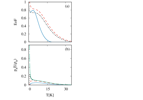
Figure 2: Entanglement of Formation as a function of temperature T for finite eigenenergies $E_{m}$ and non-zero magnetic field, $\Omega=1$, considering only non-positive values of $m$. Top and bottom panel as in Fig. 1

In Fig. 2 we show the same situation as in Fig. 1 (a), but where only blocks with non-positive values of $m$ have been taken into account. This eliminates the block with $m=K$ which has only separable eigenstates and also contains the ground state of the whole Hamiltonian. Now the ground state is also entangled which leads to a more complicated trade-off situation between the components shown in the bottom panel of the figure starting with an entangled Gibbs state at zero-temperature. The corresponding component of entanglement decays very rapidly with temperature, while all other components start to grow which leads to a plateau at small temperatures for larger $K$ and an initial growth of entanglement for $K=1$.

We have shown that the temperature-dependence of entanglement can be very diverse even in case of the simple Hamiltonian which has been studied. This fact is obvious in terms of possible behavior within a given block of the density matrix, but our study shows that the interplay of probabilities pertaining to each block can be just as important. By changing the way that temperature mixes the different blocks in the Gibbs state, we have obtained three qualitatively different scenarios, varying not only in zero-temperature entanglement, but also in monotonicity for different temperature regimes. It is important to note that the curves were obtained by qualitatively the same Hamiltonian, and a larger change was neccesary only to modify the behavior of entanglement within a single block.

VIII Conclusion

We have supplied a proof that any convex-roof entanglement measure is an average over entanglement within a given block of a density matrix which is block diagonal in such a way that individual blocks are contained within different subspaces of one of two potentially entangled subsystems (say, the environment). Although this may seem to be an overly specific regime of application, there are many Hamiltonians which possess this quality. For such Hamiltonians, any thermal-equilibrium state will inherit the same quality and the simplification of resulting calculation of entanglement can be immense. If an initial bipartite state is also block diagonal in such a way, then the evolution driven by the Hamiltonian will yield a state which retains the necessary form at any given time.

We have used the method to find the temperature-dependence of entanglement in a Gibbs state of a large system, the Hamiltonian of which is composed of a multitude of small blocks. This allowed us to show four very different behaviors of entanglement which can be occur in different parameter ranges. This can be dependent on how entanglement reacts to temperature change within each block, but it also strongly depends on the way that different blocks are mixed. We have shown that the interplay of probabilities can yield striking differences in the trends of entanglement, both in terms of entanglement at zero temperature, as well as weather it is ascending or descending in a given temperature range. Temperature driven “sudden death” type behavior is the singular property which requires “sudden death” behavior to occur within each block separately.

On the more quantum-theoretical side, our proof allows us to infer that bound entanglement cannot traverse multiple blocks; it is possible only within a single block. This has consequences for the calculation of such measures as Negativity, which cannot detect bound entanglement, making them more reliable.

Appendix A Qudit and environment with two subspaces

Here we will show that entanglement of any pure state that contains coherences between subspaces of E, eq. (15) is greater or equal to the average entanglement in its block-diagonal counterpart, eq. (23) regardless of the size of QS. Since we are now dealing with a qudit, a system of dimension $K$, the states (16) have to be substituted by

$$|\psi_{i}\rangle=\sum_{s}x_{i}^{s}|s\rangle\otimes|\varphi_{i}^{s}\rangle,$$ (34)

where the summation over $s$ spans the the qudit Hilbert space and the states $|s\rangle$ are a set of basis states on QS; $i=1,2$ still differentiates between the subspaces of E. This yields the qudit version of eq. (17),

$$|\psi\rangle=\sum_{s}a_{s}|s\rangle\otimes|\psi_{s}\rangle,$$ (35)

with

$$a_{s}=\sqrt{|\alpha|^{2}|x_{1}^{s}|^{2}+|\beta|^{2}|x_{2}^{s}|^{2}}$$ (36)

and

$$|\psi_{s}\rangle=\frac{1}{a_{s}}\left(\alpha x_{1}^{s}|\varphi_{1}^{s}\rangle+\beta x_{2}^{s}|\varphi_{2}^{s}\rangle\right).$$ (37)

The reduced density matrix of E is given by

$$\hat{\rho}_{E}=\sum_{s}a_{s}^{2}|\psi_{s}\rangle\langle\psi_{s}|$$ (38)

and the normalized linear entropy of the reduced density matrix, is

$$E(|\psi\rangle)=4\sum_{s\neq s^{\prime}}a_{s}^{2}a_{s^{\prime}}^{2}\left(1-\left|\langle\psi_{s}|\psi_{s^{\prime}}\rangle\right|^{2}\right).$$ (39)

Since the states of E from different subspaces have to be orthogonal to each other, the simplified formula for the scalar product is still valid and we have

$$\left|\langle\psi_{s}|\psi_{s^{\prime}}\rangle\right|^{2}=\frac{1}{a_{s}^{2}a_{s^{\prime}}^{2}}\left||\alpha|^{2}x_{1}^{s*}x_{1}^{s^{\prime}}\langle\varphi_{1}^{s}|\varphi_{1}^{s^{\prime}}\rangle+|\beta|^{2}x_{2}^{s*}x_{2}^{s^{\prime}}\langle\varphi_{2}^{s}|\varphi_{2}^{s^{\prime}}\rangle\right|^{2}.$$ (40)

The average of the linear entropy of the block diagonal density matrix (23) is still given by eq. (24), but with

$$E(|\psi_{i}\rangle)=4\sum_{s\neq s^{\prime}}|x_{i}^{s}|^{2}|x_{i}^{s^{\prime}}|^{2}\left(1-\left|\langle\varphi_{i}^{s}|\varphi_{i}^{s^{\prime}}\rangle\right|^{2}\right).$$ (41)

Since the formulas in both cases only differ by an identical sum over different qudit basis states, it follows that the formula (14) holds for a QS of any size.