Indirect Optimal Control of Advection-Diffusion Fields through
Robotic Swarms

Abstract

In this paper, we consider the problem of optimally guiding a large-scale swarm of underwater vehicles that is tasked with the indirect control of an advection-diffusion environmental field. The microscopic vehicle dynamics are governed by a stochastic differential equation with drift. The drift terms model the self-propelled velocity of the vehicle and the velocity field of the currents. In the mean-field setting, the macroscopic vehicle dynamics are governed by a Kolmogorov forward equation in the form of a linear parabolic advection-diffusion equation. The environmental field is governed by an advection-diffusion equation in which the advection term is defined by the fluid velocity field. The vehicles are equipped with on-board actuators that enable the swarm to act as a distributed source in the environmental field, modulated by a scalar control parameter that determines the local source intensity. In this setting, we formulate an optimal control problem to compute the vehicle velocity and actuator intensity fields that drive the environmental field to a desired distribution within a specified amount of time. In other words, we design optimal vector and scalar actuation fields to indirectly control the environmental field through a distributed source, produced by the swarm. After proving an existence result for the solution of the optimal control problem, we discretize and solve the problem using the Finite Element Method (FEM). The FEM discretization naturally provides an operator that represents the bilinear way in which the controls enter into the dynamics of the vehicle swarm and the environmental field. Finally, we show through numerical simulations the effectiveness of our control strategy in regulating the environmental field to zero or to a desired distribution in the presence of a double-gyre flow field.

1 Introduction

Given the exponential decrease in cost of electronic components over the last few decades, large collectives of robots, or robotic swarms, are becoming a viable option for a variety of missions of ever-increasing complexity, such as coverage, mapping, search-and-rescue, and surveillance (Dorigo et al., 2021). Controllers for robotic swarms should satisfy mission requirements while scaling gracefully as the number of robots $N$ increases. Mean-field models of robotic swarms (see, e.g., Elamvazhuthi and Berman (2020)) describe a swarm as a set of probability densities over space and time; since these models are independent of $N$, they can be used to design controllers for arbitrarily large swarms, with the caveat that the distribution of the swarm is controlled rather than individual robots.

In this paper, we take advantage of the mean-field model’s invariance to swarm size by using such a model to design scalable robotic swarm controllers that achieve indirect control of a distributed process that evolves according to a Partial Differential Equation (PDE), such as the concentration field of a contaminant in a fluid flow. The robots are underwater vehicles that are each equipped with an actuator that acts as a source for the process, and we aim to indirectly control the process through the coordinated motion of the swarm and the source actuation. A similar problem has previously been considered for finite teams of mobile robots, in which individual robot trajectories are controlled. For example, Cheng and Paley (2021) present an optimal control approach that uses an operator-valued Riccati equation to formulate the optimal actuation as a function of the optimal guidance, and then recast the problem in terms of the latter alone to jointly optimize the guidance of the robots and their associated actuation. Demetriou (2021) describes a path-dependent reachability approach that takes into account constraints on the robots’ motion and real-time implementation while regulating a spatially distributed process using local decentralized measurements only.

We define the indirect control problem for a distributed robotic swarm whose mean-field dynamics are modeled by a Kolmogorov forward equation in the form of a linear parabolic advection-diffusion PDE. We formulate an optimal control problem (OCP) for this mean-field model, which is coupled with the advection-diffusion dynamics of the environmental field and prove an existence theorem for the OCP using techniques for optimal control of PDEs. Then, we derive a set of first-order necessary optimality conditions and solve them numerically using a Finite Element Method (FEM) discretization. Finally, we evaluate the effectiveness of our control strategy through numerical simulations of regulation and target tracking problems in the presence of a double-gyre flow field.

2 Problem formulation

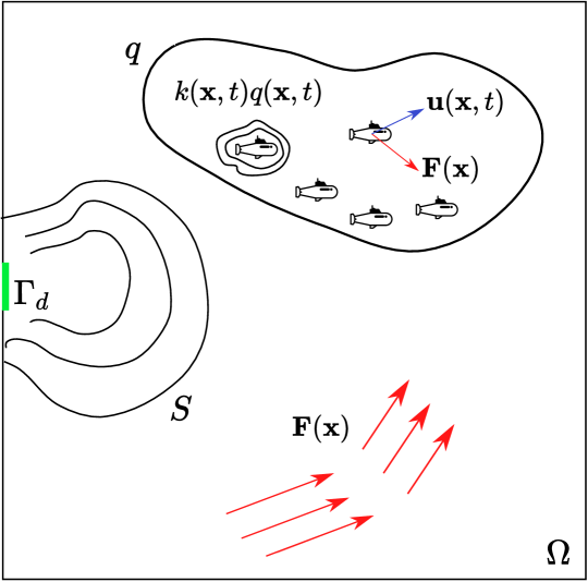
Figure 1: Illustration of the indirect control problem. The environmental field $S$ diffuses from the segment of the boundary $\Gamma_{d}$ under the advection of a fluid velocity field $\mathbf{F}$. The vehicle velocity field $\mathbf{u}$ and actuator intensity field $k$ are designed to drive $S$ to a target distribution.

We consider a swarm of robots, labeled $i=1,...,N$, that move in a bounded fluid domain $\Omega\in\mathbb{R}^{2}$. Robot $i$ occupies position $\mathbf{X}_{i}(t)\in\Omega$ at time $t$ and moves with velocity $\mathbf{v}(\mathbf{x},t)\in\mathbb{R}^{2}$, which is the sum of its self-propelled velocity $\mathbf{u}(\mathbf{x},t)$ and the fluid velocity at its position, $\mathbf{F}(\mathbf{x})$. This motion is perturbed by a 2-dimensional Wiener process $\mathbf{W}(t)$, which models stochasticity arising from inherent sensor and actuator noise or intentionally programmed “diffusive” exploratory behaviors. The robot’s position evolves according to the following Stochastic Differential Equation:

$$\begin{cases}d\mathbf{X}_{i}(t)&=~{}\mathbf{v}(\mathbf{X}_{i},t)dt+\sqrt{2D_{q}}d\mathbf{W}(t)+\mathbf{n}(\mathbf{X}_{i}(t))d\psi(t)\\ \mathbf{X}_{i}(0)&=~{}\mathbf{X}_{i,0},\end{cases}$$

where $D_{q}>0$ is a diffusion coefficient, $\mathbf{n}(\mathbf{x})$ is the unit normal to the domain boundary $\partial\Omega$ at $\mathbf{x}$, and $\psi(t)\in\mathbb{R}$ is a reflecting function, which ensures that the swarm does not exit the domain. We assume that each robot $i$ carries an on-board actuator that acts as a source of intensity $k_{i}(t)\in\mathbb{R}$ in a scalar environmental field $S(\mathbf{x},t)$, $\mathbf{x}\in\Omega$. We also assume that part of the boundary, $\Gamma_{d}\in\partial\Omega$, acts as a source with constant intensity $S_{d}$ for simplicity. The field $S$ is an advection-diffusion process with diffusion coefficient $D_{S}>0$, modeled by the following PDE problem:

$$\begin{array}[]{ll}\displaystyle\frac{\partial S}{\partial t}-D_{S}\Delta S+\mathbf{F}\cdot\nabla S=\sum_{i=1}^{N}k_{i}(t)\delta(\mathbf{x}-\mathbf{X}_{i}(t))&\textrm{in}\quad\Omega\\ \vspace{-3mm}\\ S=S_{d}\,1_{\Gamma_{d}}\quad\quad\quad\textrm{on}\quad\partial\Omega&\\ S(\mathbf{x},0)=S_{0}(\mathbf{x})\quad\textrm{on}\quad\Omega\times\{0\},&\\ \end{array}$$

where $1_{\Gamma_{d}}$ is an indicator function. The right-hand side of the PDE consists of the cumulative effect of the point sources, which have the same dynamics as the robots since they are installed on-board. Note that the explicit dependence of $S$ on space and time is omitted when clear from the context.

In the limit as $N\to\infty$, we obtain a mean-field model that describes the evolution of the probability density $q(\mathbf{x},t)$ of a single robot occupying position $\mathbf{x}$ at time $t$, or alternatively, the swarm density at this position and time. For the robot dynamics we consider here, this model takes the form of a linear parabolic advection-diffusion problem with no-flux boundary conditions; see, e.g., Sinigaglia et al. (2021). The coupled system dynamics are therefore:

$$\begin{array}[]{ll}\displaystyle\frac{\partial q}{\partial t}+\nabla\cdot(-D_{q}\nabla q+\mathbf{u}q+\mathbf{F}q)=0&\textrm{in}\quad\Omega\\ \vspace{-3mm}\\ (-D_{q}\nabla q+\mathbf{u}q+\mathbf{F}q)\cdot\mathbf{n}=0&\textrm{on}\quad\partial\Omega\\ q(\mathbf{x},0)=q_{0}(\mathbf{x})&\textrm{in}\quad\Omega\times\{0\},\\ \vspace{-1mm}\\ \displaystyle\frac{\partial S}{\partial t}-D_{S}\Delta S+\mathbf{F}\cdot\nabla S=kq&\textrm{in}\quad\Omega\\ \vspace{-3mm}\\ S=S_{d}\,1_{\Gamma_{d}}&\textrm{on}\quad\partial\Omega\\ S(\mathbf{x},0)=S_{0}(\mathbf{x})&\textrm{on}\quad\Omega\times\{0\}.\\ \end{array}$$ (1)

Note that the right-hand side of the $S$ dynamics is now the product of the intensity of the distributed actuation $k$ and the local swarm density $q$. As a consequence of this Eulerian perspective, $k=k(\mathbf{x},t)$ varies in both space and time. The robotic swarm thus aims at controlling the concentration $S$ of an advection-diffusion field through a localized actuation field $kq$ that depends on both the actuator intensity $k$ and the swarm density $q$ at each spatial location. See Figure 1 for an illustration of the problem.

Defining the state variables as $q$ and $S$, the state dynamics consists of the one-way coupled system of PDEs (1). The objective of the control problem is then to find the optimal actuation for $\mathbf{u}(\mathbf{x},t)$ and $k(\mathbf{x},t)$ to guide the space-time evolution of the field $S$ to a target distribution $z$, which may be static or dynamic, at a given time $T$. This control objective can be easily encoded in a standard quadratic cost functional of the form:

$$J=\frac{\alpha_{T}}{2}\int_{\Omega}(S(\mathbf{x},T)-z)^{2}d\Omega+\frac{\alpha}{2}\int_{0}^{T}\int_{\Omega}(S-z)^{2}d\Omega dt$$ (2)

$$~{}~{}+\frac{\beta}{2}\int_{0}^{T}\int_{\Omega}\left\lVert\mathbf{u}\right\rVert^{2}d\Omega dt+\frac{\gamma}{2}\int_{0}^{T}\int_{\Omega}k^{2}d\Omega dt,$$

where $\alpha_{T},\alpha,\beta,\gamma\geq 0$ are weighting constants. In the regulation problem, for example, we set $z=0$ and seek the optimal trade-off between effectively regulating the field $S$ and minimizing the overall energy expended by the swarm for propulsion motion and source actuation.

3 The Optimal Control Problem

In this section, we prove the existence of optimal controls, derive a system of first-order necessary optimality conditions using the Lagrangian method, and provide a consistent discretization of the OCP using the FEM.

3.1 Analysis

Both the $q$ and $S$ dynamics satisfy rather standard advection-diffusion equations of linear parabolic type; see, e.g., (Manzoni et al., 2021, Chapter 7). The natural functional space for the swarm density function $q$ which is subjected to zero-flux Neumann boundary conditions is $q\in L^{2}(0,T,H^{1}(\Omega))$, while the Dirichlet boundary suggests the choice of $\mathring{S}\in L^{2}(0,T,H^{1}_{0}(\Omega))$ for the “lifted” field variable $\mathring{S}=S-\tilde{S}_{d}$, where $\tilde{S}_{d}$ is a suitable extension of the boundary datum to the domain $\Omega$ – see, e.g., (Salsa, 2016, Chapter 8). It is also standard to select $\frac{\partial q}{\partial t}\in L^{2}(0,T,H^{1}(\Omega)^{*})$ and $\frac{\partial\mathring{S}}{\partial t}\in L^{2}(0,T,H_{0}^{1}(\Omega)^{*})$ so that the functional space for $q$ is actually $H^{1}(0,T;H^{1}(\Omega),H^{1}(\Omega)^{*})=\{y\in L^{2}(0,T;H^{1}(\Omega)):\dot{y}\in L^{2}(0,T;H^{1}(\Omega)^{*}\}$, and the same holds true for $\mathring{S}$, substituting $H^{1}$ with $H_{0}^{1}$. Therefore, we set $\mathcal{Y}=H^{1}(0,T;H^{1}(\Omega),H^{1}(\Omega)^{*})\times H^{1}(0,T;H_{0}^{1}(\Omega),H_{0}^{1}(\Omega)^{*})$ as the state space, i.e., $y=(q,S)\in\mathcal{Y}$. As done in, e.g., Roy et al. (2018) and Sinigaglia et al. (2021) for similar problems involving the Kolmogorov forward equation alone, we consider $L^{\infty}$ spaces for the control fields for which energy-like inequalities are readily available; that is, we select $\mathcal{U}=L^{2}(0,T;L^{\infty}(\Omega)^{2})\times L^{2}(0,T;L^{\infty}(\Omega))$ as the control space, so that $v=(\mathbf{u},k)\in\mathcal{U}$. Besides the choice of the functional spaces for states and controls, we make the following standard assumptions:

$$\mathbf{F}\in L^{\infty}(\Omega)^{2}$$ (A1)

$$D_{S},D_{q}>0$$ (A2)

$$S_{d}\,\,\text{is bounded}$$ (A3)

$$q_{0},S_{0}\in L^{2}(\Omega)$$ (A4)

The weak formulation of the PDE problem governing the swarm dynamics is: find $q\in L^{2}(0,T;H^{1}(\Omega))$ such that for a.e. $t\in(0,T)$,

$$\int_{\Omega}\frac{\partial q}{\partial t}\phi d\,\Omega+a_{q}(q,v;\mathbf{u})=0\vspace{1mm}$$ (4)

$$q(0)=q_{0}$$

for every $\phi\in H^{1}(\Omega)$, where

$$a_{q}(q,\phi;\mathbf{u})=\int_{\Omega}(D_{q}\nabla q\cdot\nabla\phi-(\mathbf{u}+\mathbf{F})\cdot\nabla\phi q)d\Omega.$$

The weak formulation of the PDE problem for the “lifted” variable $\mathring{S}$ is: find $\mathring{S}\,\in L^{2}(0,T;H_{0}^{1}(\Omega))$ such that for a.e. $t\in(0,T)$,

$$\int_{\Omega}\frac{\partial\mathring{S}}{\partial t}\phi\,d\Omega+a_{S}(\mathring{S},\phi)=\int_{\Omega}\,kq\,\phi\,d\Omega-a_{S}(\tilde{S}_{d},\phi)\vspace{1mm}$$ (5)

$$\mathring{S}(0)=S_{0}$$

for every $\phi\in H_{0}^{1}(\Omega)$, where

$$a_{S}(S,\phi)=\int_{\Omega}D_{S}\nabla S\cdot\nabla\phi+\mathbf{F}\cdot\nabla S\,\phi d\Omega.$$

We also define the linear functional $F\in H^{-1}=H_{0}^{1}(\Omega)^{*}$ as $F\phi=\int_{\Omega}k\,q\,\phi\,d\Omega-a_{S}(\tilde{S}_{d},\phi)$. In the following, we will need a bound on the operator norm of $F$, which we prove in the lemma below.

Lemma 1 (Bound on $F$)

Let assumptions (A1), (A2), (A3), and (A4) hold. Then the following bound on the norm of $F$ holds:

$$\left\lVert F\right\rVert_{H^{-1}(\Omega)}\leq C_{p}\left\lVert kq\right\rVert_{L^{2}(\Omega)}+(C_{p}\left\lVert\mathbf{F}\right\rVert_{L^{\infty}(\Omega)^{2}}+D_{S})\left\lVert\nabla\tilde{S}_{d}\right\rVert_{L^{2}(\Omega)},$$

where $C_{p}>0$ is the Poincarè inequality constant. From the definition of $F$ and the Cauchy-Schwarz and Poincaré inequalities, we have:

$$|F\phi|\leq\Big{(}\left\lVert kq\right\rVert_{L^{2}(\Omega)}+\left\lVert\mathbf{F}\right\rVert_{L^{\infty}(\Omega)^{2}}\left\lVert\nabla\tilde{S}_{d}\right\rVert_{L^{2}(\Omega)}\Big{)}\left\lVert\phi\right\rVert_{L^{2}(\Omega)}$$

$$+D_{S}\left\lVert\nabla\tilde{S}_{d}\right\rVert_{L^{2}(\Omega)}\left\lVert\nabla\phi\right\rVert_{L^{2}(\Omega)}$$

$$\leq C_{p}\Big{(}\left\lVert kq\right\rVert_{L^{2}(\Omega)}+\left\lVert\mathbf{F}\right\rVert_{L^{\infty}(\Omega)^{2}}\left\lVert\nabla\tilde{S}_{d}\right\rVert_{L^{2}(\Omega)}\Big{)}\left\lVert\nabla\phi\right\rVert_{L^{2}(\Omega)}$$

$$+D_{S}\left\lVert\nabla\tilde{S}_{d}\right\rVert_{L^{2}(\Omega)}\left\lVert\nabla\phi\right\rVert_{L^{2}(\Omega)}.$$

Regrouping the terms and using the definition of operator norm in $H^{-1}(\Omega)$, the result follows. ∎

Existence and well-posedness of the state dynamics follow from the well-posedness of the $q$ dynamics and basic energy estimates on the $S$ dynamics. This is a consequence of the one-way coupling from $q$ to $S$. Following the same arguments as in Sinigaglia et al. (2021), we have that

$$\left\lVert q\right\rVert^{2}_{H^{1}(0,T;H^{1}(\Omega),H^{1}(\Omega)^{*})}\leq C_{0}(\left\lVert\mathbf{u}\right\rVert^{2})\left\lVert q_{0}\right\rVert^{2}_{L^{2}(\Omega)}.$$

To prove the well-posedness of the $S$ dynamics, we note that $kq\in L^{2}(0,T;L^{2}(\Omega))$ since

$$\left\lVert kq\right\rVert_{L^{2}(0,T;L^{2}(\Omega))}^{2}\leq\left\lVert k\right\rVert_{L^{2}(0,T;L^{\infty}(\Omega))}^{2}\left\lVert q\right\rVert_{L^{2}(0,T;L^{2}(\Omega))}^{2}$$

$$\hskip 14.22636pt\leq C\left\lVert k\right\rVert_{L^{2}(0,T;L^{\infty}(\Omega))}^{2}\left\lVert\mathbf{u}\right\rVert_{L^{2}(0,T;L^{\infty}(\Omega)^{2})}^{2},$$

and the latter quantity in the inequality is bounded by the definition of the control space $\mathcal{U}$. Therefore, $S$ satisfies an advection-diffusion equation with $L^{2}$ right-hand side for which existence and uniqueness results are available – see, e.g., (Salsa, 2016, Theorem 9.9).

A number of standard a priori estimates can be derived for the $S$ dynamics as well; see, e.g., (Manzoni et al., 2021, Theorem 7.1). In particular, it can be shown that

$$\left\lVert S\right\rVert_{L^{2}(0,T;H_{0}^{1}(\Omega))}^{2}\leq\frac{e^{2\lambda T}}{\alpha_{0}}\Big{(}\left\lVert S_{0}\right\rVert_{L^{2}(\Omega)}^{2}+\frac{1}{\alpha_{0}}\left\lVert F\right\rVert_{L^{2}(0,T;H^{-1}(\Omega))}^{2}\Big{)},$$

where $\lambda=\frac{\left\lVert\mathbf{F}\right\rVert^{2}_{L^{\infty}(\Omega)^{2}}}{D_{S}}$ and $\alpha_{0}=\min\{\frac{D_{S}}{2},\frac{\left\lVert\mathbf{F}\right\rVert^{2}_{L^{\infty}(\Omega)^{2}}}{2\,D_{S}}\}$. From Lemma 1 and the bounds on $\left\lVert kq\right\rVert_{L^{2}(0,T;L^{2}(\Omega)}$, it is clear that $\left\lVert S\right\rVert_{L^{2}(0,T;H_{0}^{1}(\Omega))}$ is bounded by the control norms on $\mathbf{u}$ and $k$. Regarding $\dot{S}=\frac{\partial S}{\partial t}$, we have that

$$\left\lVert\dot{S}\right\rVert_{L^{2}(0,T;H^{-1}(\Omega))}^{2}~{}\leq C_{0}\left\lVert S_{0}\right\rVert_{L^{2}(\Omega)}^{2}+$$

$$~{}~{}~{}~{}(\frac{C_{0}}{\alpha_{0}}+2)\left\lVert F\right\rVert_{L^{2}(0,T;H^{-1}(\Omega))}^{2},$$

where $C_{0}=\frac{2}{\alpha_{0}}e^{2\lambda T}(D_{S}+C_{p}\left\lVert\mathbf{F}\right\rVert_{L^{\infty}(\Omega)^{2}})^{2}$, since both $\left\lVert\dot{S}\right\rVert_{L^{2}(0,T;H^{-1}(\Omega))}$ and $\left\lVert S\right\rVert_{L^{2}(0,T;H_{0}^{1}(\Omega))}$ are bounded by the control norms. Therefore, we can conclude that

$$\left\lVert S\right\rVert^{2}_{H^{1}(0,T;H_{0}^{1}(\Omega),H^{-1}(\Omega))}$$

$$=\left\lVert\dot{S}\right\rVert_{L^{2}(0,T;H^{-1}(\Omega))}^{2}+\left\lVert S\right\rVert^{2}_{L^{2}(0,T;H_{0}^{1}(\Omega))}$$

$$\leq f(\left\lVert k\right\rVert_{L^{2}(0,T;L^{\infty}(\Omega))},\left\lVert\mathbf{u}\right\rVert_{L^{2}(0,T;L^{\infty}(\Omega)^{2})}),$$

which will turn out to be useful in the proof of existence of optimal controls.

We define the control-to-state operator as the map $(S,q)=\Xi[\mathbf{u},k]$ which associates to each control function $v\in\mathcal{U}$ with a corresponding state $y\in\mathcal{Y}$. The following result regarding the Fréchet differentiability of the control-to-state operator is also needed to prove existence of optimal controls.

Lemma 2 (Differentiability of the control-to-state map)

Let assumptions (A1), (A2), (A3), and (A4) hold. Then the control-to-state map $(S,q)=\Xi[\mathbf{u},k]$ is Fréchet differentiable and the directional derivative $(z_{S},z_{q})=\Xi^{\prime}[\mathbf{u},k](\mathbf{h},l)$ at $(\mathbf{u},k)\in\mathcal{U}$ in the direction $(\mathbf{h},l)\in\mathcal{U}$ is the solution of the coupled PDE system:

$$\begin{array}[]{ll}\displaystyle\frac{\partial z_{q}}{\partial t}+\nabla\cdot(-D_{q}\nabla z_{q}+\mathbf{u}z_{q}+\mathbf{F}z_{q})=-\nabla\cdot(\mathbf{h}\,q)&\textrm{in}\quad\Omega\\ \vspace{-3mm}\\ (-D_{q}\nabla z_{q}+\mathbf{u}z_{q}+\mathbf{F}z_{q})\cdot\mathbf{n}=-\mathbf{h}\cdot\mathbf{n}\,q&\textrm{on}\quad\partial\Omega\\ \vspace{-2mm}\\ z_{q}(\mathbf{x},0)=0&\textrm{in}\quad\Omega\times\{0\},\\ \vspace{1mm}\\ \displaystyle\frac{\partial z_{S}}{\partial t}-D_{S}\Delta z_{S}+\mathbf{F}\cdot\nabla z_{S}=kz_{q}+lq&\textrm{in}\quad\Omega\\ \vspace{-2mm}\\ z_{S}=0&\textrm{on}\quad\partial\Omega\\ z_{S}(\mathbf{x},0)=0&\textrm{on}\quad\Omega\times\{0\}.\\ \end{array}$$

(Sketch) The derivation of the equations governing the sensitivity $z_{q}$ of the swarm dynamics, and bounds on the norm of $z_{q}$, can be found e.g. in Roy et al. (2018) and Sinigaglia et al. (2021). On the other hand, the expression for the dynamics of $z_{S}$ can be obtained by formally computing the directional derivative, that is, the limit $\lim_{s\to 0}\frac{S(\mathbf{u}+s\mathbf{h},k+sl)-S(\mathbf{u},k)}{s}$. Bounds on $z_{S}$ are obtained by adapting the above results on the norm of $S$, and noting that by the triangular inequality, $\left\lVert kz_{q}+lq\right\rVert_{L^{2}(0,T;L^{2}(\Omega))}\leq\left\lVert kz_{q}\right\rVert_{L^{2}(0,T;L^{2}(\Omega))}+\left\lVert lq\right\rVert_{L^{2}(0,T;L^{2}(\Omega))},$ so that continuity of the sensitivity $z_{q}$ and $z_{S}$ with respect to variations of the control functions $\mathbf{h}$, $l$ can be easily obtained, thus proving the differentiability of the control-to-state map. ∎

We are now ready to prove a result concerning the existence of optimal controls.

Theorem 3 (Existence of optimal controls)

Let assumptions (A1), (A2), (A3), and (A4) hold. Then there exists an optimal control $\bar{v}=(\bar{\mathbf{u}},\bar{k})$ that minimizes the cost functional (2) subject to the dynamics (1), that is, $\bar{y}=(\bar{S},\bar{q})=\Xi[\bar{\mathbf{u}},\bar{k}]$.

(Sketch) Existence results for bilinear optimal control problems involving the Kolmogorov forward equation with space-time dependent controls have been proved in Sinigaglia et al. (2021), Roy et al. (2018), and references therein. Choosing a minimizing sequence $(\mathbf{u}_{n},k_{n})$, due to the weak* sequential compactness of the control space, we have that

$$\mathbf{u}_{n}\stackrel{{\scriptstyle*}}{{\rightharpoonup}}\bar{\mathbf{u}}\quad\text{ (weakly star) in }L^{2}(0,T;L^{\infty}(\Omega)^{2})$$

$$k_{n}\stackrel{{\scriptstyle*}}{{\rightharpoonup}}\bar{k}\quad\text{ (weakly star) in }L^{2}(0,T;L^{\infty}(\Omega))$$

Due to the bounds on $S$ and $q$, we also have that the resulting sequence $(S_{n},q_{n})=\Xi[\mathbf{u}_{n},q_{n}]$ is bounded and thus weakly convergent in $\mathcal{Y}$ to $(\bar{S},\bar{q})\in\mathcal{Y}$, see e.g. (Evans, 2010, Appendix S, Theorem 3). It remains to prove that:

$$\int_{0}^{T}\int_{\Omega}\,k_{n}q_{n}\,\phi\,d\Omega\,dt\to\int_{0}^{T}\int_{\Omega}\,\bar{k}\bar{q}\,\phi\,d\Omega\,dt$$

for each $\phi\in L^{2}(0,T;H_{0}^{1}(\Omega))$. To this end, we write

$$\int_{0}^{T}\int_{\Omega}\left(k_{n}q_{n}-\bar{q}\bar{k}\right)\phi d\Omega dt$$

$$=\int_{0}^{T}\int_{\Omega}\bar{q}\phi\left(k_{n}-\bar{k}\right)d\Omega dt+\int_{0}^{T}\int_{\Omega}\left(q_{n}-\bar{q}\right)k_{n}\phi\,d\Omega dt.$$

Since $\bar{q}\phi\in L^{2}(0,T;L^{1}(\Omega))$, the dual of $L^{2}(0,T;L^{\infty}(\Omega))$, and $k_{n}\stackrel{{\scriptstyle*}}{{\rightharpoonup}}\bar{k}$, the first integral tends to zero by Lebesgue’s dominated convergence theorem. To analyze the second integral, we use the Aubin-Lions Lemma (see, e.g., (Manzoni et al., 2021, Appendix A, Theorem A.19)) to ensure that $q_{n}\to\bar{q}$ strongly in $L^{2}(0,T;L^{2}(\Omega))$. Then we obtain:

$$|\int_{0}^{T}\int_{\Omega}\left(q_{n}-\bar{q}\right)k_{n}\phi\,d\Omega dt|\leq$$

$$\left\lVert k_{n}\right\rVert_{L^{2}(0,T;L^{\infty}(\Omega))}\left\lVert\phi\right\rVert_{L^{2}(0,T;L^{2}(\Omega))}\left\lVert q_{n}-\bar{q}\right\rVert_{L^{2}(0,T;L^{2}(\Omega))}=0.$$

Since $\Omega$ is bounded, the weak* convergence of $\mathbf{u}_{n}\in L^{2}(0,T;L^{\infty}(\Omega)^{2})$ to some $\bar{\mathbf{u}}\in L^{2}(0,T;L^{\infty}(\Omega)^{2})$ implies weak convergence of $\mathbf{u}_{n}$ to $\bar{\mathbf{u}}$ in $L^{2}(0,T;L^{2}(\Omega)^{2})$. The same holds for $k$; that is, $k_{n}$ weakly converges to $\bar{k}$ in $L^{2}(0,T;L^{2}(\Omega))$. Then, exploiting the fact that $S_{n}$ weakly converges to $\bar{S}$ in $L^{2}(0,T;H_{0}^{1}(\Omega))$ and that $J(S,\mathbf{u},k)$ is convex and continuous in $L^{2}(0,T,H_{0}^{1}(\Omega))\times L^{2}(0,T;L^{2}(\Omega)^{2})\times L^{2}(0,T;L^{2}(\Omega))$, we conclude that

$$J(\bar{S},\bar{\mathbf{u}},\bar{k})\leq\lim_{n\to\infty}\inf J(S_{n},\bar{\mathbf{u}}_{n},k_{n})=\inf J.$$

Therefore, the pair $(\bar{y},\bar{v})$ is an optimal pair for the considered optimal control problem. ∎

We note that uniqueness of an optimal solution is not guaranteed, due to the bilinear way in which both controls $\mathbf{u}$ and $k$ enter into the coupled system dynamics.s

3.2 Optimality Conditions

We now derive a system of first-order necessary optimality conditions using the Lagrangian multipliers method. For the problem at hand, the Lagrangian can be defined as

$$\mathcal{L}=J-\int_{0}^{T}\int_{\Omega}\lambda_{q}\left(\frac{\partial q}{\partial t}+\nabla\cdot(-D_{q}\nabla q+\mathbf{u}q)\right)d\Omega dt$$ (6)

$$~{}~{}~{}~{}~{}+\int_{0}^{T}\int_{\Omega}\lambda_{S}\left(kq-\frac{\partial S}{\partial t}+D_{S}\Delta S\right)d\Omega dt.$$

Note that we have defined adjoint fields $\lambda_{q}$ and $\lambda_{S}$ that are related to the state dynamics of both $q$ and $S$. The adjoint dynamics for $\lambda_{q}$ and $\lambda_{S}$ thus satisfy:

$$\begin{array}[]{ll}\displaystyle-\frac{\partial\lambda_{q}}{\partial t}-D_{q}\Delta\lambda_{q}-\mathbf{u}\cdot\nabla\lambda_{q}=k\,\lambda_{S}&\textrm{in}\quad\Omega\\ \vspace{-3mm}\\ \nabla\lambda_{q}\cdot\mathbf{n}=0&\textrm{on}\quad\partial\Omega\\ \lambda_{q}(\mathbf{x},T)=0&\textrm{in}\quad\Omega\times\{T\},\\ \vspace{-2mm}\\ \displaystyle-\frac{\partial\lambda_{S}}{\partial t}-D_{S}\Delta\lambda_{S}-\mathbf{F}\cdot\nabla\lambda_{S}=\alpha\,(S-z)&\textrm{in}\quad\Omega\\ \vspace{-3mm}\\ \lambda_{S}=0&\textrm{on}\quad\partial\Omega\\ \lambda_{S}(\mathbf{x},T)=\alpha_{T}\,(S(\mathbf{x},T)-z)&\textrm{in}\quad\Omega\times\{T\},\\ \end{array}$$

which are obtained by taking the first variation of the Lagrangian along variations in swarm density $q$ and the environmental field $S$, respectively. Note that the coupling between the adjoint fields is dual with respect to the state dynamics. The coupling is from $q$ to $S$ in the state system, while it is from $\lambda_{S}$ to $\lambda_{q}$ in the adjoint system. The dual of the forcing term $k\,q$ in the $S$ dynamics is the forcing term $k\lambda_{S}$ in the $\lambda_{q}$ dynamics.

The reduced gradients of $J$ with respect to $\mathbf{u}$ and $k$ can therefore be expressed as

$$\begin{array}[]{l}\nabla J_{\mathbf{u}}=\beta\mathbf{u}+q\,\nabla\lambda_{q},\\ \nabla J_{k}=\gamma k+q\,\lambda_{S},\end{array}$$ (7)

by taking the first variations of the Lagrangian in the directions of $\mathbf{u}$ and $k$, respectively. Note that, despite $k$ entering linearly into the $S$ dynamics, the reduced gradient $\nabla J_{k}$ depends on the dynamics of the swarm density $q$. This is a consequence of the multiplicative nature of the $S$ forcing term $k\,q$.

3.3 Numerical Discretization

The OCP with coupled system dynamics (1) is discretized in the state variables $S$ and $q$ using the Finite Element Method (FEM). The discretized state dynamics are

$$\begin{array}[]{l}M_{q}\dot{\mathbf{q}}+\Big{(}A_{q}-B_{\mathbf{F}}^{\top}-\mathbb{B}^{\top}\mathbf{u}\Big{)}\mathbf{q}=\mathbf{0}\\ M_{S}\dot{\mathbf{S}}+\Big{(}A_{S}-B_{\mathbf{F}}^{\top}\Big{)}\mathbf{S}=\mathbb{C}\mathbf{k}\mathbf{q}\\ \mathbf{q}(0)=\mathbf{q}_{0}\\ \mathbf{S}(0)=\mathbf{S}_{0},\end{array}$$ (8)

where $\mathbb{B}$ is the rank-3 transport coefficient tensor defined by $\mathbb{B}_{ijk}=\int_{\Omega}\frac{\partial\phi_{j}}{\partial x}\phi_{i}\,\phi_{k}\,d\Omega$; $\mathbb{B}\mathbf{u}$ is the tensor vector product defined by $(\mathbb{B}\mathbf{u})_{ij}=\sum_{k=1}^{N_{u}}\mathbb{B}_{ijk}\,u_{k}$; $\mathbb{C}$ is the reaction tensor defined by $\mathbb{C}_{ijk}=\int_{\Omega}\phi_{j}\phi_{i}\,\phi_{k}\,d\Omega$; and $M$, $B$, and $A$ are the usual FEM mass, transport, and stiffness matrices, respectively.

The discretization of the adjoint system is:

$$\begin{array}[]{l}-M_{q}\dot{\boldsymbol{\lambda}}_{q}+\Big{(}A_{q}-B_{\mathbf{F}}-\mathbb{B}\mathbf{u}\Big{)}\boldsymbol{\lambda}_{q}=\mathbf{k}\mathbb{C}^{\top}\boldsymbol{\lambda}_{S}\\ -M_{S}\dot{\boldsymbol{\lambda}}_{S}+A_{S}\boldsymbol{\lambda}_{S}=\alpha\,M_{S}(\mathbf{S}-\mathbf{z})\\ \boldsymbol{\lambda}_{q}(T)=\mathbf{0}\\ \boldsymbol{\lambda}_{S}(T)=\alpha_{T}M_{S}(\mathbf{S}(T)-\mathbf{z}).\\ \end{array}$$ (9)

Finally, the reduced gradient discretization is:

$$\begin{array}[]{l}\nabla J_{\mathbf{u}}=\beta M_{u}\mathbf{u}+\mathbf{q}^{\top}\mathbb{B}\boldsymbol{\lambda}_{q}\\ \vspace{-4mm}\\ \nabla J_{\mathbf{k}}=\gamma M_{k}\mathbf{k}+\mathbf{q}^{\top}\mathbb{C}^{\top}\boldsymbol{\lambda}_{S}.\end{array}$$ (10)

We can apply the same reasoning as in Sinigaglia et al. (2021) to perform numerical gradient computation. Therefore, we use the Discretize-then-Optimize (DtO) approach (see e.g., (Manzoni et al., 2021, Chapter 8)) to numerically solve the problem while avoiding inconsistencies in the gradient computation. In order to do so, the discrete Lagrangian must be computed and differentiated. This computation, which is very similar to the one in our previous work (see Sinigaglia et al. (2021) for a more detailed treatment of the problem for the swarm dynamics alone), is not reported here due to space constraints.

Since the coupling is one-way, at each time step we advance the dynamics of the swarm density $q$ and then solve the problem for $S$. Using similar reasoning, we first solve the discrete adjoint dynamics with respect to $\lambda_{S}$, and then the adjoint problem for $\lambda_{q}$. It can be checked that carrying out the optimization at the continuous level and then discretizing the optimality conditions, that is, adopting the Optimize-then-Discretize (OtD) approach, results in the same system of equations at the semi-discrete level; up to choosing a suitable time-discretization, the two approaches fully commute.

4 Simulation Results

In this section, we present numerical simulation results that show the effectiveness of our control strategy. The computational domain $\Omega=[0,1]^{2}$ is discretized into a triangular mesh with $N_{s}=2,788$ degrees of freedom, and the time interval $[0,T]$ is discretized into $N_{t}=61$ time steps, where the final time is $T=1.5(s)$. The resulting fully discrete optimization problem has 510,204 control variables and 170,068 state variables. A steady double-gyre flow field is chosen as the fluid velocity field $\mathbf{F}$.

Using the DtO method, the reduced gradient is computed with respect to the control variables only. Computations are carried out in MATLAB using a modified version of the redbKit (Quarteroni et al. (2015)) library to assemble the FEM matrices and tensors and the Tensor Toolbox (Bader and Kolda (2006)) to perform efficient tensor computations. The nonlinear optimization software Ipopt (Wächter and Biegler (2006)) is then used to solve the resulting nonlinear optimization problem.

Two test cases are considered. In Test Case 1, we solve a regulation problem with target distribution $z=0$ and the Dirichlet boundary condition illustrated in Figure 1, with $S=S_{d}=10$ along $\Gamma_{d}$. Test Case 2 is a tracking problem with $z=S_{0}(\mathbf{x})$ and a homogeneous Dirichlet boundary condition. In Figure 2, we compare the controlled and uncontrolled dynamics of the total mass of the environmental field $S$, defined as $m_{S}(t)=\int_{\Omega}S(\cdot,t)d\Omega$, for the two test cases. For Test Case 1, the uncontrolled steady-state value of $m_{S}(t)$ depends on the equilibrium balance between the mass generated along $\Gamma_{d}$ and the mass absorbed along the rest of the boundary. In the controlled case, however, the robotic swarm drives $m_{S}(t)$ to zero through coordinated motion, defined by their self-propelled velocity $\mathbf{u}$, and the intensity $k$ of their distributed actuation. In Test Case 2, the uncontrolled mass $m_{S}(t)$ exponentially converges to zero due to diffusion and the homogeneous Dirichlet boundary condition, while the controlled mass $m_{S}(t)$ is driven to $\int_{\Omega}S_{0}(\cdot)d\Omega$ due to the efforts of the swarm to maintain $S$ at its initial condition $S_{0}(\mathbf{x})$. Figure 3 shows snapshots of the swarm density dynamics under the action of the controls and the fluid velocity field for Test Case 1. Figure 4 compares snapshots of the controlled and uncontrolled dynamics of $S$ for Test Case 1, and Figure 5 presents snapshots of the optimal actuation $k$ for this case. Finally, snapshots of the controlled dynamics of $S$ for Test Case 2 are shown in Figure 6.

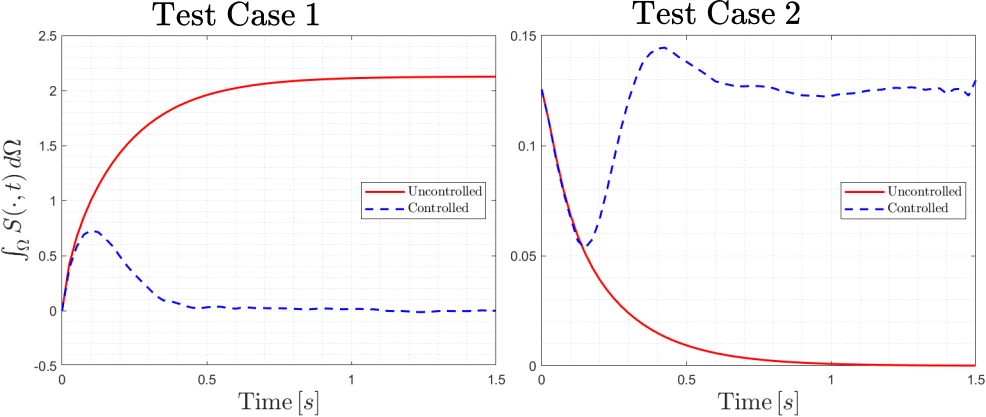
Figure 2: Controlled and uncontrolled dynamics of the total environmental field mass for both test cases. After a common transient phase during which the robotic swarm moves toward where its actuation is most effective, the controlled dynamics are driven to the total mass of the target distribution $z$.

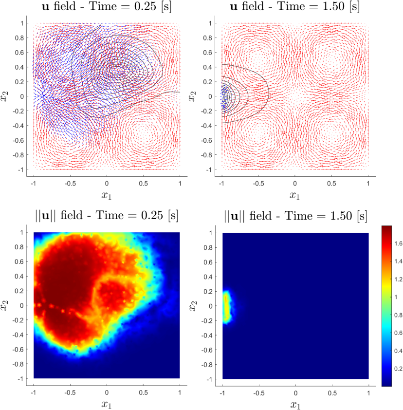
Figure 3: Test Case 1. Top: Swarm density contours (black), optimal robot velocity control $\mathbf{u}(\mathbf{x},t)$ (blue), and fluid velocity field $\mathbf{F}$ (red) at times $t=0.25(s)$ and $t=1.5(s)$. Bottom: Euclidean norm $||\mathbf{u}||$ of the optimal control, with a maximum value of $\sqrt{2}$.

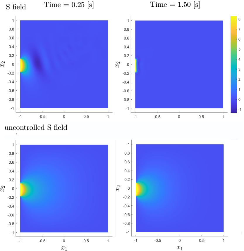
Figure 4: Test Case 1. Controlled (top) and uncontrolled (bottom) environmental field $S(\mathbf{x},t)$ at times $t=0.25(s)$ and $t=1.5(s)$.

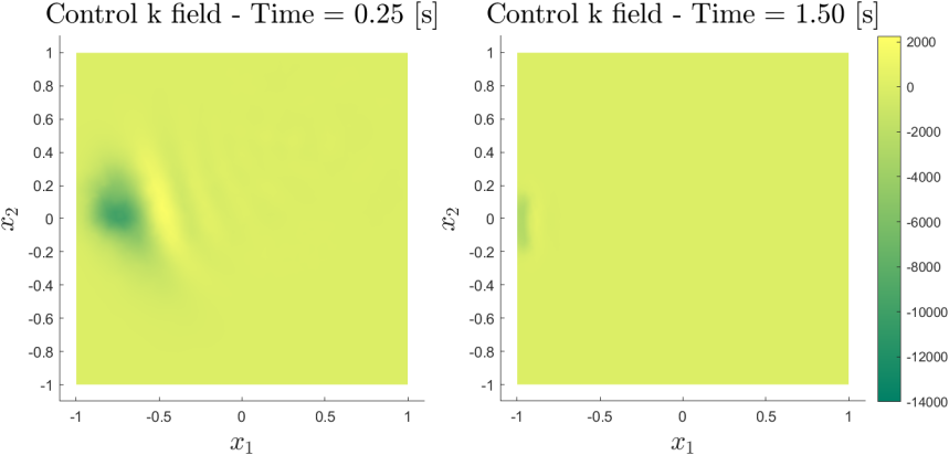
Figure 5: Test Case 1. Optimal actuation $k(\mathbf{x},t)$ at times $t=0.25(s)$ and $t=1.5(s)$. The distributed actuation $k$ is correlated with the swarm density $q$.

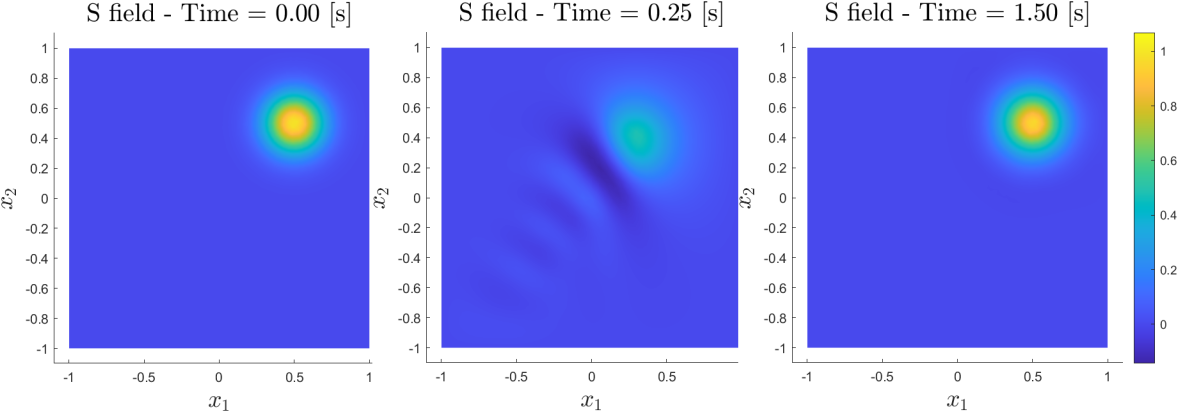
Figure 6: Test Case 2. Controlled environmental field $S(\mathbf{x},t)$ at times $t=0(s)$, $t=0.25(s)$, and $t=1.5(s)$. For the sake of brevity, the uncontrolled dynamics are not shown since they exhibit a trivial diffusion to zero due to the homogeneous Dirichlet boundary condition.

References

- Bader and Kolda (2006) Bader, B.W. and Kolda, T.G. (2006). Algorithm 862: MATLAB tensor classes for fast algorithm prototyping. ACM Trans. Math. Softw., 32(4), 635–653.
- Cheng and Paley (2021) Cheng, S. and Paley, D.A. (2021). Optimal control of a 2D diffusion–advection process with a team of mobile actuators under jointly optimal guidance. Automatica, 133, 109866.
- Demetriou (2021) Demetriou, M.A. (2021). Controlling 2D PDEs using mobile collocated actuators-sensors and their simultaneous guidance constrained over path-dependent reachability regions. In 2021 American Control Conference (ACC), 1491–1496. IEEE.
- Dorigo et al. (2021) Dorigo, M., Theraulaz, G., and Trianni, V. (2021). Swarm Robotics: Past, Present, and Future. Proceedings of the IEEE, 109(7), 1152–1165.
- Elamvazhuthi and Berman (2020) Elamvazhuthi, K. and Berman, S. (2020). Mean-field models in swarm robotics: A survey. Bioinspiration and Biomimetics, 15(1), 015001.
- Evans (2010) Evans, L.C. (2010). Partial Differential Equations. American Mathematical Society.
- Manzoni et al. (2021) Manzoni, A., Salsa, S., and Quarteroni, A. (2021). Optimal Control of Partial Differential Equations. Analysis, Approximation, and Applications, volume 207 of Applied Mathematical Sciences. Springer.
- Quarteroni et al. (2015) Quarteroni, A., Manzoni, A., and Negri, F. (2015). Reduced Basis Methods for Partial Differential Equations: An Introduction. Springer International Publishing.
- Roy et al. (2018) Roy, S., Annunziato, M., Borzì, A., and Klingenberg, C. (2018). A Fokker–Planck approach to control collective motion. Computational Optimization and Applications, 69(2), 423–459.
- Salsa (2016) Salsa, S. (2016). Partial differential equations in action: from modelling to theory, volume 99. Springer.
- Sinigaglia et al. (2021) Sinigaglia, C., Manzoni, A., and Braghin, F. (2021). Density control of large-scale particles swarm through PDE-constrained optimization. URL http://arxiv.org/abs/2104.06373.
- Wächter and Biegler (2006) Wächter, A. and Biegler, L.T. (2006). On the implementation of an interior-point filter line-search algorithm for large-scale nonlinear programming. Mathematical programming, 106(1), 25–57.