Beyond Gaussian processes: Flexible Bayesian modeling and inference for geostatistical processes

Abstract

This paper proposes a novel family of geostatistical models to account for features that cannot be properly accommodated by traditional Gaussian processes. The family is specified hierarchically and combines the infinite-dimensional dynamics of Gaussian processes with that of any multivariate continuous distribution. This combination is stochastically defined through a latent Poisson process and the new family is called the Poisson-Gaussian Mixture Process - POGAMP. Whilst the attempt of defining geostatistical processes by assigning some arbitrary continuous distribution to be the finite-dimension distributions usually leads to non-valid processes, the finite-dimensional distributions of the POGAMP can be arbitrarily close to any continuous distribution and still define a valid process. Formal results to establish the existence and some important properties of the POGAMP, such as absolute continuity with respect to a Gaussian process measure, are provided. Also, an MCMC algorithm is carefully devised to perform Bayesian inference when the POGAMP is discretely observed in some space domain.

Key Words: Heavy tails; MCMC; Skewness; Poisson process.

Universidade Federal de Minas Gerais, Brazil

1 Introduction

Continuous spatial statistical modelling, referred to as geostatistics, is an appealing approach to explain the probabilistic dynamics of some response variable observed on some continuous domain. Spatial prediction is an important problem in fields such as petroleum engineering, civil engineering, mining, geography, geology, environmental, hydrology and climate studies (Dubrule,, 1989; Hohn,, 1998; Cressie,, 2015; Bevilacqua et al.,, 2021). Geostatistical problems consider a partial realization of an underlying random field, indexed by locations, that vary (typically) continuously on a fixed domain in space and focus on understanding the stochastic dynamics of the generating process to predict values at unobserved locations or regions. The underlying random field is often assumed to be a Gaussian processes (GP). This assumption facilitates prediction and provides some justification for the use of the spatial prediction. A GP is completely characterized by its mean and covariance functions and the GP measure implies that the joint distribution of the process at any finite collection of locations is a multivariate normal. The stability of the multivariate normal distribution under summation and conditioning offers tractability and simplicity, besides having closure under marginal and conditional distributions.

The GP inherits appealing properties of the normal distribution, making it a strong and convenient candidate to solve numerous problems and case studies in real life. Nevertheless, in practice, the normality assumption might not be appropriate to fit some observed phenomena, especially in the presence of heavy tailed or skewness behaviors. This motivates the development of more general classes of geostatistical models that allow for non-Gaussian features whist preserving some desirable properties of GPs.

The problem of modeling skewed data in a geostatistics context has been a subject of interest in recent years. In particular, the question whether multivariate skewed distributions can be consistently extended to random fields is of great interest in many spatial and spatiotemporal applications. The skew-normal class of distributions extends the widely employed normal distributions by introducing a skewing function and shares many statistical properties of the latter. Several classes of multivariate skew distributions have been proposed in the literature, such as the skew-normal (Azzalini and Valle,, 1996) and skew-t Azzalini and Capitanio, (2003) distributions.

Basically, previously proposed non-Gaussian geostatistical processes are based on one of two general strategies. The first one attempts to define the process by setting its finite-dimensional distributions (FDD), typically some class of parametric distributions, for example, skew-normal or skew-t. This approach, however, may lead to a non-valid process, in the sense of not defining a probability measure. Mahmoudian, (2018) provides the necessary conditions for a skew-normal distribution to define a valid process and points out a few ill-defined processes in the literature, such as the ones in Kim and Mallick, (2004), Allard and Naveau, (2007), Hosseini et al., (2011) and Zareifard and Khaledi, (2013). The authors also present some examples of valid processes by basically considering process that can be written as a (non-linear) measurable function of one or more Gaussian processes (and possibly some finite-dimensional random variables). In particular, the SUN family (Arellano-Valle and Azzalini,, 2006) that unifies all extension of the SN family requires considerable restriction to its parametric space in order to define a valid process.

The second general strategy to define non-Gaussian processes is by considering (measurable) non-linear transformations of one or more independent Gaussian processes. The validity of the GPs guarantees the validity of the resulting process. De Oliveira et al., (1997), for example, used non-linear monotone parametric transformations to define non-Gaussian random fields. Palacios and Steel, (2006) proposed the Gaussian-log-Gaussian model, which is based on a log-Gaussian scale mixture of a Gaussian process in its most general form. The resulting process is able to accommodate heavy tail behavior and is a function of two independent Gaussian processes. Alodat and Al-Rawwash, (2009) proposes a skew-Gaussian process by taking a function of a Gaussian process and a univariate standard normal random variable. Later on, Alodat and AL-Rawwash, (2014) allows the second component to have a non-zero mean to define the extended skew Gaussian process. Bevilacqua et al., (2021) also proposed a process with heavy tail behavior by considering a scale mixture of a GP where the mixture process is a function of $\nu$ independent GPs, where $\nu$ is the degrees of freedom parameter of the resulting student-t marginal FDD. The multivariate FDDs though are unknown. The authors obtain the density for the bivariate case but this depends on an intractable (infinite sum) term. The authors also propose a process to account for skewness and heavy tails by replacing the GP in the aforementioned process by the skew Gaussian process of Zhang and El-Shaarawi, (2010), which itself is a function of two independent GPs. The resulting process is has skew-t marginals but, naturally, shares the same intractability problems as the previous process. The authors even mention that “it is apparent that likelihood-based methods for the skew-Gaussian process are impractical from computational point of view even for a relatively small dataset”. Tagle et al., (2020) proposed a spatial Skew-$t$ model that relies on a partition of the spatial domain and is a function of a GP and a finite collection of random variables with distributions gamma, half-normal and multivariate normal. Their model has discontinuities at the boundaries and assumes conditional independence among points for different regions.

A general framework to define transformations of GPs is through Gaussian copulas. It has the advantage of allowing the choice of any arbitrary marginal distribution whilst the dependence structure is define by the chosen copula. Other than Gaussian copulas may also be considered in order to desire to have more complex dependence structures but these usually lead to intractable densities and moments. Examples of geostatistical processes defined through copulas can be found in Bárdossy, (2006); Bárdossy and Li, (2008); Kazianka and Pilz, (2010, 2011); Prates et al., (2015); Hughes, (2015); Gräler et al., (2010); Gräler and Pebesma, (2011).

Whilst considering transformations of GPs allows for the definition of valid non-Gaussian processes, it has some considerable drawbacks. First of all, relying on multiple copies of Gaussian process have a considerable impact on the derivation and computational cost of inference methodologies (including prediction). Second, important features such as densities and moments (uni and bivariate) are typically complicated and sometimes even intractable/unavailable. Third, achieving tractability may come at a cost of compromising model flexibility. Finally, some models may have serious identifiability issues (see Genton and Zhang,, 2012).

Recently, Zheng et al., (2021) proposed a new direction to define scalable non-Gaussian processes by considering a nearest neighbor formulation and setting the respective conditional finite-dimensional distributions to be a mixture of conditional distributions induced by bivariate joint ones. The formulation is quite general but features like FDDs and moments are only available for a few simpler cases. Furthermore, defining a process with the desired flexible properties using the proposed structure is not straightforward.

Motivated by the limitations and complexity of the existing literature on non-Gaussian geostatistical processes, this paper aims at proposing a flexible family of processes that can properly accommodate non-Gaussian features such as skewness and heavy tails, in a parsimonious and interpretable way. The conceptualization of the process is based on the choice of a family of multivariate continuous distribution that has the desirable features for the resulting process. The proposed process is constructed in a way that any continuous multivariate distribution can be considered and its impact on the resulting process is clear and intuitive. The process is specified hierarchically, through an augmented Poisson process (PP), such that the FDD at the locations of the PP are given by the initially chosen multivariate distribution. Furthermore, conditional on the value of the process at those locations, the probability measure of the infinite-dimensional remainder is a Gaussian measure. This feature implies appealing properties of the resulting process and, ultimately, facilitates the computation in simulation and inference contexts.

Inspired by its particular hierarchical structure, the proposed family is called the Poisson-Gaussian Mixture Process - POGAMP. The main advantages of the POGAMP are: 1) its existence is guaranteed, despite the multivariate distribution initially chosen; 2) it is highly flexible in terms of modelling since its finite-dimensional distributions are some sort of mixture between normal and the chosen multivariate distribution and can get arbitrarily close to the latter when the rate of the augmented PP increases. Other important features of the POGAMP are its absolutely continuity w.r.t. the Gaussian measure, which basically means that all the almost sure (a.s.) properties of the latter are inherited by the POGAMP, such as continuity and differentiability, and the possibility to use conditionally independence-based structures in a straightforward way to apply the POGAMP to large datasets. Typical choices for the multivariate distribution used as basis for the POGAMP include skew-normal, student-t, skew-t, copulas.

From an inference perspective, we propose an MCMC algorithm to perform Bayesian inference based on the observation of a POGAMP in a finite collection of locations in a compact domain $S$. The algorithm consists of an infinite-dimensional Markov chain that converges to the posterior distribution of all the unknown quantities of the model. The infinite-dimensionality of the chain is due to the same property of the POGAMP and requires the use of non-standard simulation techniques and MCMC updates to devise a valid, exact and efficient MCMC algorithm. The term “exact” refers to the property that the limiting distribution of the MCMC chain is the exact (infinite-dimensional) target posterior distribution. The exactness property is achieved by employing a simulation technique called retrospective sampling.

The contributions of methodology proposed in this paper can be generally described to be twofold. First, it allows for the definition of flexible valid processes with FDDs arbitrarily close to any multivariate distribution and also with the level of proximity to that distribution varying across the considered domain. Second, even in the cases where the chosen multivariate distribution defines a valid process, the POGAMP construction may facilitate the derivation of more efficient inference methodologies.

This paper is organized as follows. Section $2$ presents the POGAMP, establishes its existence and provides results related to its main properties. Section $3$ presents the MCMC algorithm to perform Bayesian inference for discretely observed POGAMPs. Section 4 presents a nearest neighbor GP approach to deal with large datasets.

2 A novel family of geostatistical models

2.1 The Poisson-Gaussian Mixture Process

The Poisson-Gaussian Mixture Process is hierarchically defined through conditional and marginal measures. This not only allows for a tractable way to define the model, but also gives good intuition about its dynamics and a clear interpretation of its components. The definition of a joint probability measure using a decomposition into conditional and marginal measures, however, does not guarantee the existence of the former. The existence of the joint measure needs to be established in order to yield the existence of the marginal geostatistical process of interest. The formal definition of the POGAMP is provided in Definition 2 below and its existence is established in Theorem 1. Before defining the POGAMP, we present the definition of a Gaussian process.

Definition 1.

A Gaussian process $Y$ is a stochastic process in some space domain $S\in R^{d}$, $d\in\mathds{N}$, such that, for all $n\geq 1$ and $(s_{1},\dots,s_{n})\in S^{n}$,

$$(Y(s_{1}),\dots,Y(s_{n}))\sim N_{n}(\mu(s_{1},\ldots,s_{n}),\Sigma(s_{1},\ldots,s_{n})),$$

where $\mu(s_{1},\ldots,s_{n})\in\mathds{R}^{d}$ and $\Sigma(s_{1},\ldots,s_{n})$ is a $n\times n$ positive-definite covariance matrix.
If $\mu(s_{1},\ldots,s_{n})$ is a constant vector, $cov(Y(s_{i}),Y(s_{i}))=\sigma^{2}\in\mathds{R}^{+}$, $\forall$ $i$, and $cov(Y(s_{i}),Y(s_{j}))=\sigma^{2}\rho(|s_{i}-s_{j}|)$, $\forall$ $i\neq j$ and some correlation function $\rho$, the Gaussian process is said to be stationary and isotropic.

Definition 2.

The Poisson-Gaussian Mixture Process - POGAMP. Let $(Y,N)$, for $Y=\{Y(s),s\in S\subset\mathds{R}^{2}\}$, for a compact domain $S$, be a coordinate process on $(\mathcal{Y}\times\mathcal{N},\sigma(\mathcal{B}(\mathcal{Y})\times\mathcal{B}(\mathcal{N})))$, where $\mathcal{Y}$ is the Banach space of continuous functions on $S\in\mathds{R}^{d}$ and $\mathcal{B}(\mathcal{Y})$ is the Borel $\sigma$-algebra generated by the open sets of $\mathcal{Y}$ in the strong topology. $\mathcal{N}$ is the locally compact separable metric space of point patterns in $S$, such that no two points are in the same location and the number of points in any compact subset of $S$ is finite, with $\sigma$-algebra $\mathcal{B}(\mathcal{N})$. Now define $\mathcal{P}$ as the probability measure on $(\mathcal{Y}\times\mathcal{N},\sigma(\mathcal{B}(\mathcal{Y})\times\mathcal{B}(\mathcal{N})))$ under which
i) $N$ is a Poisson process on $S$ with non-negative intensity function $\lambda:=\{\lambda(s),s\in S\}$ and events $S_{N}:=\{\dot{s}_{1},\ldots,\dot{s}_{|N|}\}$;
ii) conditional on $N$, $Y_{N}:=(Y(S_{N,1}),\ldots,Y(S_{N,|N|}))$ has Lebesgue probability density function $f_{N}$, such that $f_{N}$ is continuous on $(S_{N},Y_{N})\in(S^{|N|}\times\mathcal{X}^{|N|})$ and uniformly integrable w.r.t. the $N$-dimensional Lebesgue measure, where $\mathcal{X}\subset\mathds{R}$ is the support of each coordinate of $f_{N}$;
iii) conditional on $(N,Y_{N})$, $Y$ is a Gaussian Process with mean $\mu$ and covariance function $\Sigma$ on $S\setminus S_{N}$.

We shall refer to the Gaussian process that defines the conditional process in $iii)$ as the base GP. The spatial process $Y$ from the POGAMP is considerably general and flexible, given the flexibility to specify the density $f_{N}$ and the intensity function $\lambda$. Specific POGAMP models are defined in terms of the class of distributions $f$, that defines $f_{N}$ for each possible value of $N$, and the intensity function (IF) $\lambda$. For example, one may consider $f$ to be a multivariate Skew-t distribution with an isotropic covariance function.

The components $f$ and $\lambda$ have clear purposes in the definition of the POGAMP. The former ought to have the features desired for the finite-dimensional distributions of the $Y$, for example, skewness and heavy tails. The intensity function $\lambda$ stochastically defines how close the FDDs of $Y$ should be to $f$ and how this similarity should vary across the space. Intuitively, the FDDs of $Y$ are some sort of mixture between $f$ and a normal distribution and the IF $\lambda$ determines the (possibly continuously varying) “weight” of each of the two distributions in the mixture. For smaller values of $\lambda$, $Y$ approaches the GP characteristics whilst, for larger values, $Y$ approaches $f$ (in the sense of its FDDs approaching $f$). We shall consider either the homogeneous case, i.e., $\lambda(s)=\lambda\in\mathds{R}^{+}$, $\forall s$, or the non-homogeneous case with a parametric IF $\lambda(s)=\lambda(s;\theta_{\lambda})$, for some parameter vector $\theta_{\lambda}$. More general (non-parametric) IFs may be used by incorporating existing methodologies for exact inference for non-parametric and non-homogeneous Poisson processes such as Gonçalves and Gamerman, (2018) and Gonçalves and Dias, (2022).

The uniform integrability condition for $f$ is used to establish the limiting result in Theorem 2, from Section 2.2, regarding the weak convergence of the finite-dimensional distributions of the POGAMP to $f$. This is a quite mild condition which is typically satisfied (for example, by the skew-t distribution). A generally easy to check condition is that $f^{1+\delta}$, for a $\delta>0$, is Lebesgue integrable.

We will focus on the case where $S\subset\mathbbm{R}^{2}$ as it is considered in most of the geostatistical applications. The following theorem establishes the existence of the POGAMP.

Theorem 1.

Existence of the POGAMP. $\mathcal{P}$, as defined in Definition 2, is a probability measure on $(\mathcal{Y}\times\mathcal{N},\sigma(\mathcal{B}(\mathcal{Y})\times\mathcal{B}(\mathcal{N})))$, which implies that $Y$ (under $\mathcal{P}$) is a valid stochastic process.

The proof of Theorem 1 relies on the following Lemma.

Lemma 1.

Let $(\Omega_{1},\mathcal{F}_{1},\mu_{1})$ be a probability space such that, for each $\omega_{1}\in\Omega_{1}$, there exists a probability measure $\mu_{2,\omega_{1}}$ on $(\Omega_{2},\mathcal{F}_{2})$. Consider the joint measurable space $(\Omega,\sigma(\mathcal{F}))$, where $\Omega=\Omega_{1}\times\Omega_{2}$ and $\mathcal{F}=\mathcal{F}_{1}\times\mathcal{F}_{2}$, and suppose that

$$g_{A}(\omega_{1})=\int_{\Omega_{2}}\mathbbm{1}[(\omega_{1},\omega_{2})\in A]d\mu_{2,\omega_{1}}(\omega_{2}),\text{ is $\mathcal{F}_{1}$-measurable, $\forall A\in\mathcal{F}$.}$$

Then, there exists a probability measure $\mu$ on $(\Omega,\sigma(\mathcal{F}))$ that satisfies

$$\mu(A)=\int_{\Omega_{1}}\int_{\Omega_{2}}\mathbbm{1}[(\omega_{1},\omega_{2})\in A]d\mu_{2,\omega_{1}}(\omega_{2})d\mu_{1}(\omega_{1}),\quad\forall A\in\mathcal{F},\quad\omega_{1}\in\Omega_{1}\quad\text{and}\quad\omega_{2}\in\Omega_{2},$$

and $\mu$ is called the joint measure.

Lemma 1 provides the conditions required for the pair composed of a marginal and a conditional probability measures to define a valid joint probability measure. The Lemma considers a general framework, unlike the versions found in the literature which only consider finite-dimensional real measurable spaces. The proofs of Lemma 1 and Theorem 1 are presented in Appendix A.

2.2 Properties of the POGAMP

We now explore some important properties of the POGAMP which have direct impact on its use in a statistical context. First, let $\mathcal{G}$ be the probability measure on $(\mathcal{Y}\times\mathcal{N},\sigma(\mathcal{B}(\mathcal{Y})\times\mathcal{B}(\mathcal{N})))$ that differs from $\mathcal{P}$ only on the distribution of $N$ and $(Y_{N}|N)$ such that, under $\mathcal{G}$, $N$ is a unit rate homogeneous PP on $S$ and $(Y_{N}|N)$ has the normal distribution induced by base GP of the POGAMP. We shall refer to the process $(Y,N)$ under $\mathcal{G}$ as the augmented GP, since the induced marginal measure of $Y$ is the base GP. Note that its existence is established by Theorem 1.

Proposition 1.

$\mathcal{P}$ is absolutely continuous w.r.t. $\mathcal{G}$ with Radon-Nikodym derivative given by $\cfrac{\displaystyle f}{\displaystyle g}(Y_{N})$, where $g$ is the Lebesgue density of $Y_{N}$ under $\mathcal{G}$.

An equivalent statement to that in Proposition 1 is that $\mathcal{G}$-a.s implies $\mathcal{P}$-a.s. As a consequence, interesting features of GPs, such as a.s. continuity and a.s. differentiability of the generated surfaces, are inherited by the POGAMP. The result in the proposition also has relevant implications in the derivation and validity of an MCMC algorithm to perform inference for discretely-observed POGAMPs.

Another interesting consequence of Proposition 1 is that the Kullback Lieber divergence between $\mathcal{P}$ and $\mathcal{G}$ depends on $Y$ only through $Y_{N}$.

Proposition 2.

The Kullback Lieber divergence between the POGAMP and the augmented GP measures is given by

$$D_{\text{KL}}(\mathcal{P}\parallel\mathcal{G})=\sum_{n=0}^{\infty}\cfrac{\rm{e}^{-\Lambda_{S}}(\Lambda_{S})^{n}}{n!}\int_{S^{n}}\int_{\mathds{R}^{n}}\prod_{j=1}^{n}\frac{\lambda(s_{j})}{\Lambda_{S}}\log\left(\cfrac{f_{N}}{g_{N}}(y)\right)f_{N}(y)\text{d}y\text{d}s,$$

where $\Lambda_{S}=\int_{S}\lambda(s)ds$, $s=(s_{1},\ldots,s_{|N|})$, $y=(y_{1},\ldots,y_{|N|})$ and $f_{N}$ and $g_{N}$ are the conditional density of $Y$ at $s$, under $\mathcal{P}$ and $\mathcal{G}$, respectively, given $N$. If $N$ is a homogeneous PP with rate $\lambda$,

$$D_{\text{KL}}(\mathcal{P}\parallel\mathcal{G})=\sum_{n=0}^{\infty}\cfrac{\rm{e}^{-\lambda\mu(S)}\lambda^{n}}{n!}\int_{S^{n}}\int_{\mathds{R}^{n}}\log\left(\cfrac{f_{N}}{g_{N}}(y)\right)f_{N}(y)\text{d}y\text{d}s$$

The proofs of the propositions 1 and 2 are given in Appendix A.

As it was mentioned before, one of the main advantages of the POGAMP is that its finite-dimensional distributions inherit the characteristics of some chosen class of multivariate distribution $f$ and it is a valid process under some very mild conditions. In fact, as the IF of $N$ increases, the FDDs get arbitrarily close to $f$, as it is stated in the following theorem.

Theorem 2.

Consider a monotonic sequence of positive real numbers $\{\lambda_{n}\}_{n=1}^{\infty}$ such that $\lambda_{n}\uparrow\infty$ and $(\lambda_{n+1}-\lambda_{n})>\epsilon>0$, $\forall n\in\mathds{N}$. Let $S_{R}$ be a set of any $r$ distinct locations in $S$, for $r\in\mathbbm{N}$ and define an infinite sequence of POGAMPs with common $f$ distribution, such that the component $N$ of the $n$-th POGAMP is a Poisson process with intensity function $\lambda_{n}(s)\geq\lambda_{n}$, $\forall s\in S$. Define $Y_{n,R}$ as the component $Y$ of the $n$-th POGAMP at locations $S_{R}$ and $Y_{f,R}$ as the $r$-dimensional random variable with distribution $f$ at $S_{R}$. Then, $Y_{n,R}\xrightarrow{\makebox[20.00003pt][c]{$\scriptstyle d$}}Y_{f,R}$.

The proof of Theorem 2 is given in Appendix A.

Note that, in the cases that $f$ defines a valid process, the POGAMP can get arbitrarily close to this (at least in terms of the FDDs) by increasing the rate $\lambda$, with the advantage of having the tractability of the Gaussian process measure. Furthermore, even if $f$ does not define a valid process, the POGAMP can still have FDD arbitrarily close to $f$. Finally, the existence of the POGAMP allows us to perform likelihood-based inference for discretely-observed spatial phenomena, under that model. Figure 1 illustrates the result in Theorem 2 by showing the empirical marginal density of the POGAMP at the centroid of a square of size 10, for different values of $\lambda$, when the $f$ distribution is skew-normal, student-t and skew-t.

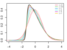
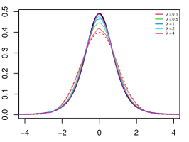
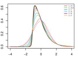
Figure 1: Empirical density of the POGAMP at the centroid of a square with side 10 for skew-normal, student-t and skew-t $f$ distributions, for different values of $\lambda$. Black line if the marginal $f$ density and dashed red line is the marginal density of the base GP.

Standard calculations based on the hierarchical structure of the POGAMP are used to obtain the density of its finite-dimensional distributions. We shall we ${\pi}$ as a general notation for densities. If this refers to a discrete or a continuous finite-dimensional random variable, the implicit dominating measure is the counting or the Lebesgue measure, respectively.

Proposition 3.

Density of the finite-dimensional distributions. For any finite collection of locations $S_{R}$, the density ${\pi}_{R}$ of $Y_{R}$ ($Y$ at $S_{R}$), under the POGAMP measure, is given by

$$\displaystyle{\pi}_{R}(y) =\sum^{\infty}_{n=0}w_{n}g(y;n),$$ (1)

$$\mbox{where\;\;\;}\displaystyle w_{n} =\frac{\left[\Lambda_{S}\right]^{n}}{n!}c_{n},\;\;\;\;\;\displaystyle g(y;n)=\frac{g^{*}(y;n)}{c_{n}},$$

$$c_{n}=\int_{\mathbbm{R}^{n}}g^{*}(y;n)\text{d}y,\;\;\;\;\;g^{*}(y;n) =\int_{S^{n}}{\pi}(s|n)\int_{\mathbbm{R}^{n}}f_{N}(x\mid s,n){\pi}_{\mathcal{G}}(y\mid x,s,n)\text{d}x\text{d}s,$$

with $s$ and $x$ being $n$-dimensional vectors, ${\pi}(s|n)=\prod_{j=1}^{n}\frac{\lambda(s_{j})}{\Lambda_{S}}$, $f_{N}(x\mid s,n)$ being the density of the $f$ distribution at locations $s$ and ${\pi}_{\mathcal{G}}(y\mid x,s,n)$ being the density of $Y$ at locations $S_{R}$, conditional on $(Y_{N},S_{N},|N|)=(y,s,n)$, under the base GP measure.

Note that the marginal density of $Y_{R}$ is a discrete mixture of the conditional (on $|N|$) densities $g$.

Now we express the covariance function of $Y$, under the POGAMP measure.

Proposition 4.

Let $s_{1}$ and $s_{2}$ be any two locations in $S$, $\Sigma_{i}$ be the row vector of the covariances between $Y(s_{i})$ and $Y(S_{N})$ under the base GP, for $i=1,2$, and $\Sigma_{N}$ and $\Sigma_{N,f}$ be the covariance matrix of $Y_{N}$ under the the base GP and the $f$ distribution, respectively. Then,

$$Cov(Y_{1},Y_{2})=\mathrm{E}[Cov(Y_{1},Y_{2}|Y_{N})]+\mathrm{E}[\Sigma_{1}\Sigma^{-1}_{N}\Sigma_{N,f}(\Sigma_{2}\Sigma^{-1}_{N})^{T}].$$ (2)

If, additionally, the covariance function is the same under the base GP and $f$, we have that

$$Cov(Y_{1},Y_{2})=\rho(s_{1},s_{2})$$ (3)

where $\rho(s_{1},s_{2})$ is the covariance of $(Y(s_{1}),Y(s_{2}))$, under the base GP.

The proof of Proposition 4 is presented in Appendix A.

The second result in Proposition 4 has important practical implications as it provides an analytical representation of the covariance function of the POGAMP, allowing for a clear interpretation of this.

Finally, we state an interesting property regarding symmetry of the POGAMP. First, consider the following definitions.

Definition 3.

Symmetry of a compact region. We say that a compact region $S\in\mathds{R}^{2}$ is symmetric if there exists at least one rotation of $\mathds{R}^{2}$, that is not a multiple of $2\pi$, for which $S$ remains the same.

Definition 4.

Symmetry of a Poisson process. We say that a Poisson process $N$ on a symmetric region $S\in\mathds{R}^{2}$ is symmetric if all the rotations of $\mathds{R}^{2}$ that preserve $S$, also preserve the intensity function of $N$.

Definition 5.

Symmetry of locations. Suppose that $S$ and $N$ are symmetric and let $\mathbf{s}$ and $\mathbf{s}^{\prime}$ be two sets of $r$ locations in $S$, for any $k\in\mathds{N}$. We say that $\mathbf{s}$ and $\mathbf{s}^{\prime}$ are symmetric w.r.t. $(S,N)$ if, for at least one of the rotations defined in Definition 3, $\mathbf{s}$ in the rotated space is equal to $\mathbf{s}^{\prime}$ in the non-rotated one.

Proposition 1.

Suppose that $f$ is stationary and $S$ and $N$ is symmetric. Then, for any two sets $\mathbf{s}$ and $\mathbf{s}^{\prime}$ in $S$ that are symmetric w.r.t. $(S,N)$, we have that $Y(\mathbf{s})\overset{d}{=}Y(\mathbf{s}^{\prime})$, under the POGAMP measure.

The proof of the Proposition 1 is presented in Appendix A.

We present three examples of the symmetry property of the POGAMP. In Figure 2-(a), $N$ is a homogeneous PP and the four sets of points defined by the different colours are symmetric between themselves. In Figure 2-(b), the intensity function of $N$ is piecewise constant, and the blue and red sets are symmetric and the black and green ones also are. In Figure 2-(c), the intensity function of $N$ is proportional to a bivariate normal density function with symmetry at the centroid. In this case, the four sets of points defined by the different colours are symmetric between themselves.

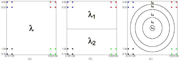
Figure 2: Examples of the symmetry property of the POGAMP.

2.3 Model specification and identifiability

The wide range of possibilities to choose the $f$ distribution and the intensity function $\lambda$ defines the POGAMP as a very general and flexible class of geostatistical models. As a consequence, issues such as model specification and identifiability become an important aspect when considering the POGAMP for statistical analysis. As in every statistical modelling problem, model parsimony is to be considered to specify the model to be fit. A reasonable balance between flexibility and predictive capability ought to be pursued.

Naturally, the main step when specifying a POGAMP is the choice of $f$. This distribution ought to possess all the non-Gaussian features one wants the final model to have, such as skewness and heavy tails. The FDDs of the POGAMP are some sort of mixture of $f$ and the FDDs of the base GP, therefore, knowing features of $f$ such as densities and moments is crucial to understand the dynamics of the resulting process.

An important issue to be explored is whether moments (marginal and joint) of the $f$ distribution and the base GP should be matched, in particular, mean, variance and covariance function. This has a direct impact on the number of parameters in the model and, consequently, on model parsimony. Matching those moments should typically be a reasonable strategy, specially if a stationary behavior is expected from the fitted model. On the other hand, non-stationary behaviors can be considered in terms of similarity with $f$ across the space domain, by considering a non-constant IF $\lambda$, and in terms of moments/covariance structure, by not matching those properties between $f$ and the base GP, with non-constant $\lambda$. One can also consider a non-stationary $f$ distribution.

Well-known classes of skew and heavy tail distributions ought to be a typical choice for $f$. For example, skew-Normal, student-t, skew-t and copula-based distributions. We call the attention to more general classes of distributions for which the process with FDDs given by $f$ is ill-defined. For example, general classes of skew-normal and skew-t distributions and non-Gaussian copula-based distributions. Finite mixtures of distributions are also an attractive possibility. In particular, mixtures of distributions with fixed levels of skewness and heavy tails may be a good alternative to avoid the estimation of parameters that define those features, whereas the level of skewness and heavy tails can be still estimated through the estimation of the mixture weights (see Bispo et al.,, 2020). Finally, spatial covariates to explain the mean of the process can be introduced by simply defining $Y(s)=f(\mathbf{X}(s);\theta)+\zeta(s)$, where $f$ some suitable function of a set of spatial covariates $\mathbf{X}$ and parameters $\theta$, and $\zeta$ is a POGAMP with mean 0.

Model identifiability is of particular concern in terms of the trade-off between level of departure from normality by $f$ and closeness between the POGAMP Fdds and $f$ (magnitude of $\lambda$). For example, a non-Gaussian feature such as heavy tails or skewness may be increasingly incorporated to the POGAMP by enhancing those features in $f$ or by increasing $\lambda$. In particular, suppose that $f$ is a t distribution and so the heavy tail behavior of the POGAMP can be adjusted by changing the degrees of freedom parameter of $f$ or the value of $\lambda$ for a fixed $f$ with considerably heavy tails (see Figure 3). This does not necessarily mean that the same distribution can be obtained for different settings of those two characteristics, but very similar ones certainly can. Therefore, in a limited data size scenario, the amount of information may not be enough to avoid practical identifiability problems.

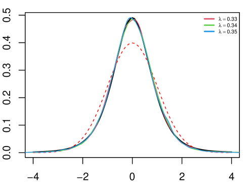
Figure 3: Empirical marginal density of the POGAMP with a student-t $f$ with degrees of freedom 3 for different combinations of $\lambda$. Black line is the density of a student-t with degrees of freedom 5.

A reasonable way to tackle the identifiability issue under the Bayesian approach is by considering robust penalising priors. In the context described in the previous paragraph, we ought to favor scenarios with the lowest $\lambda$, motivated by the consequent gains in computational cost. Nevertheless, devising a penalizing prior prior for $\lambda$ that is robust in terms of model specification and data size is not trivial, even if considering sophisticate classes of penalising priors such as the penalise complex priors (PC priors) of Simpson et al., (2017). That is because we cannot specify a base distribution in closed form in terms of $\lambda$ - not even for the marginal densities of the POGAMP. Instead, we consider a penalizing prior for the complexity parameters of the $f$ distribution, i.e., the parameters that define the departure from Gaussianity. For example, degrees of freedom and skewness parameters.

For a given complexity parameter $\xi$ indexing the $f$ distribution, we define a base value $\xi_{0}$ that defines the most complex accepted distribution $f$. The PC prior on $\xi$ is given by

$$\pi(\xi)=\zeta e^{-\zeta d(\xi,\xi_{0})}\left|\frac{\partial d(\xi,\xi_{0})}{\partial\xi}\right|,$$ (4)

where $d(\xi,\xi_{0})=\sqrt{2KLD(\xi,\xi_{0})}$, with $KLD(\xi,\xi_{0})$ being the Kullback-Leibler divergence between the marginal $f$ under $\xi$ and under $\xi_{0}$, i.e.,

$$KLD(\xi,\xi_{0})=\int_{\mathds{R}}f(x|\xi)\log\left(\frac{f(x|\xi)}{f(x|\xi_{0})}\right)dx.$$ (5)

We typically need to resort to numerical approximations to compute (5).

3 MCMC

Performing statistical inference for infinite-dimensional models - when the dimension of the unknown quantities of the model (parameters and latent variables) is infinitely uncountable, is a highly complex problem. For many years, solutions had to rely on discrete (finite-dimensional) approximations of those quantities. This naturally represents a significant source of error in the analysis and this error is typically hard to be measured and/or controlled. The advances in computational methods, specially Monte Carlo under a Bayesian approach, have brought a new perspective to deal with infinite-dimensional problems by allowing for an analysis where no discretisation error is involved, only Monte Carlo one. The latter is much simpler to quantify and control, resulting in more precise and computationally efficient analyses.

Exact (free of discretisation error) inference solutions for infinite-dimensional problems are possible mainly due to a neat simulation technique called retrospective sampling. It basically allows to deal with infinite-dimensional random variables by unveiling only a finite-dimensional representation of this, which has two main properties: i) it is enough to know its value in order to execute the steps of the algorithm in context, for example, MCMC; ii) any finite-dimensional part of the infinite-dimensional remainder of that r.v. can be simulated conditional on it. The idea of retrospective sampling in the context of simulation of infinite-dimensional r.v.’s was introduced in Beskos and Roberts, (2005) to perform exact simulation of diffusion paths. It was later used in a statistical context in several works (see, for example, Beskos et al., (2006) and Gonçalves and Gamerman, (2018)).

We propose an infinite-dimensional MCMC algorithm that relies on retrospective sampling to perform exact Bayesian inference for discretely-observed POGAMPs. The algorithm consists of a Gibbs sampling with Metropolis-Hastings steps and is exact in the sense of having the exact posterior of all the unknown quantities in the model as its invariant distribution. Each step of the algorithm is carefully designed to be computationally efficient and provide feasible and reasonable solutions to the inference problem at hand. The infinite dimensionality of the algorithm is due to the same property of the component $Y_{u}$.

Suppose that a POGAMP $Y$ is observed at some finite collection of locations $s_{1},\ldots,s_{n}$ in $S$. The vector of unknown quantities to be estimated is given by $\psi=(N,Y_{N},Y_{u},\theta_{G},\theta_{f},\lambda)$, where $Y_{u}=Y\setminus(Y_{N},Y_{o})$ and $Y_{o}=(Y_{s_{1}},\ldots,Y_{s_{n}})$. Vectors $\theta_{G}$ and $\theta_{f}$ are the sets of parameters indexing the base GP and $f$ distribution, respectively.

Under the Bayesian paradigm, inference about $\psi$ is based on the posterior distribution of $(\psi\mid Y_{o})$, which has a density, w.r.t. a suitable dominating measure, proportional to

$${\pi}(Y_{o},\psi) ={\pi}_{\mathcal{G}}(Y_{u}\mid Y_{N},Y_{o},\theta_{G}){\pi}_{\mathcal{G}}(Y_{o}\mid Y_{N},\theta_{G})f_{N}(Y_{N}\mid\theta_{f},N){\pi}(N\mid\lambda){\pi}(\lambda,\theta_{f},\theta_{G}),$$ (6)

where ${\pi}_{\mathcal{G}}$ refers to the respective densities w.r.t. to the base GP measure.

Our Gibbs sampling algorithm considers the following blocking scheme:

$$N,\;\;\;Y_{N},\;\;\;\lambda,\;\;\;\theta_{G},\;\;\;\theta_{f},\;\;\;Y_{u}.$$

Retrospective sampling is employed so that the Markov chain can be simulated by unveiling $Y_{u}$ only at a finite (though random) collection of locations at each iteration of the Gibbs sampler. Furthermore, blocks $Y_{N}$ and $\theta_{G}$ are sampled via collapsed Gibbs sampling (see Liu,, 1994), by integrating out $Y_{u}$.

3.1 Sampling $Y_{N}$

By integrating out $Y_{u}$, we have that

$${\pi}(Y_{N}\mid\cdot)\propto{\pi}_{\mathcal{G}}(Y_{o}\mid Y_{N},N,\theta_{G})f_{N}(Y_{N}\mid N,\theta_{f}).$$ (7)

We are unable to sample directly from the density above, so we resort to a Metropolis-Hastings step. The proposal distribution is a Gaussian random walk, properly tuned to have an acceptance rate of approximately $0.234$ (see Roberts et al.,, 1997), assuming that its dimension is greater than $5$. The acceptance probability of a move $Y_{N}\rightarrow Y_{N}^{*}$ is given by

$$\alpha(Y_{N},Y_{N}^{*})=1\land\cfrac{f_{N}(Y_{N}^{*}\mid N,\theta_{f}){\pi}_{\mathcal{G}}(Y_{o}\mid Y_{N}^{*},N,\theta_{G})}{f_{N}(Y_{N}\mid N,\theta_{f}){\pi}_{\mathcal{G}}(Y_{o}\mid Y_{N},N,\theta_{G})}.$$ (8)

Since the locations of $N$ change along the MCMC chain, it is not possible to use an empirical covariance matrix of the chain in the random walk proposal. Instead, we define the covariance matrix of the proposal to be proportional to the corresponding matrix under the $f$ distribution, for parameter values given by the average of those parameters over last $M$ iterations of the chain. This is done a couple of times for some suitable value of $M$ (around 500) at every $M$ iterations of the chain. The multiplication factor of the covariance matrix of the proposal is tuned so to reach the desired acceptance rate.

3.2 Sampling $N$

The full conditional density of $N$ is proportional to

$${\pi}(N\mid\cdot)\propto{\pi}_{\mathcal{G}}(Y_{u},Y_{o}\mid Y_{N},\theta_{G})f_{N}(Y_{N}\mid\theta_{f},N){\pi}(N\mid\lambda).$$ (9)

We update $N$ via MH with proposal distribution given by the Poisson process prior $PP(\lambda)$. This, however, may lead to poor mixing as the mean value of $|N|$ gets higher. In order to mitigate this problem, we divide $S$ into $K$ regular squares and use that same proposal in each of those squares. The value of $K$ is chosen empirically in terms of the mixing properties and computational cost of the algorithm.

The acceptance probability of a move $N_{k}\rightarrow N_{k}^{*}$, for $N$ in the $k$-th sub-region, is given by

$$\alpha(N_{k},N_{k}^{*}) =1\land\cfrac{{\pi}_{\mathcal{G}}(Y_{N_{k}}\mid Y_{N^{*}},\theta_{G})f_{N}(Y_{N_{k}^{*}}\mid Y_{N_{\setminus k}},\theta_{f})}{{\pi}_{\mathcal{G}}(Y_{N_{k}^{*}}\mid Y_{N},\theta_{G})f_{N}(Y_{N_{k}}\mid Y_{N_{\setminus k}},\theta_{f})},$$ (10)

where $Y_{N_{k}}$ is $Y$ at the locations from $N_{k}$ and $Y_{N_{\setminus k}}$ is $Y$ at the locations from all the $N_{j}$’s, for $j\neq k$.

Whenever a $N_{k}$ is updated, a few specific steps need to be performed. First, it is required to simulate $Y$ at the proposed locations $N_{k}^{*}$, from the base GP conditional distribution of $(Y_{N_{k}^{*}}|Y_{N},Y_{o})$, for which the inverse of the covariance matrix of $(Y_{N},Y_{o})$, under the base GP, is required. Second, the inverse covariance matrix of $Y_{N_{\setminus k}}$, under the $f$ distribution, is computed in order obtain the values of the two $f$ densities in (10). Third, the inverse covariance matrix of $Y_{N^{*}}$, under the base GP, is computed in order obtain the value of the ${\pi}_{\mathcal{G}}$ density in the numerator of (10). Finally, the inverse covariance matrix of $Y_{N}$, under the base GP, is computed in order obtain the value of the ${\pi}_{\mathcal{G}}$ density in the denominator of (10). This last matrix has already been computed as it is used on the update step of $Y_{N}$. The same matrix, under the $f$ distribution, has also been computed from the update step of $\theta_{f}$. In order to optimise the computational cost in the computation of the other three matrices, we note that they all consist of the respective inverse covariance of vectors of locations that are either a subset or contain the locations for which the inverse covariances have already been computed. This allows us to use the latter ones to obtain the former ones at a (typically) much lower cost. The two matrix operations required to do so are explained in Appendix B.

Furthermore, we perform a virtual step after updating each $N_{k}$. In theory, this consists in updating $Y_{u}$ from its full conditional distribution, which is defined by base GP conditional on $(Y_{o},Y_{N})$. In practice, due to the retrospective sampling approach, this simply means that any finite set of $Y_{u}$ currently sampled is discarded. Those sets basically consist of $Y$ at the previous $N_{k}$ when an acceptance occurred or at a rejected proposal. Finally, note the infinite dimensionality of the MCMC chain together with the retrospective sampling of $Y_{u}$ avoids the use of a (complicated) reversible jump step to update $(N,Y_{N})$.

3.3 Sampling $\lambda$, $\theta_{G}$ and $\theta_{f}$

For the case in which $N$ is a homogeneous PP with rate $\lambda$, standard conjugate Bayesian analysis calculations imply that, for a prior distribution $Gamma(\alpha_{\lambda},\beta_{\lambda})$, the full conditional distribution of $\lambda$ is a $Gamma(\alpha_{\lambda}+|N|,\beta_{\lambda}+\mu(S))$.

If $N$ is non-homogeneous with a parametric IF $\lambda(s;\theta_{\lambda})$, the full conditional density of $\theta_{\lambda}$ is proportional to

$$\exp\left\{-\int_{S}\lambda(s;\theta_{\lambda})ds\right\}\prod_{j=1}^{|N|}\lambda(s_{N,j};\theta_{\lambda}){\pi}(\theta_{\lambda}),$$ (11)

for some prior ${\pi}(\theta_{\lambda})$. If a conjugate analysis is not feasible, $\theta_{\lambda}$ is updated via ordinary Gaussian random walk MH.

Both $\theta_{G}$ and $\theta_{f}$ are sampled via MH steps with properly tuned Gaussian random walk proposals (see Roberts and Rosenthal,, 2009). The respective acceptance probabilities are given by

$$\alpha(\theta_{G},\theta_{G}^{*}) =1\land\cfrac{{\pi}(Y_{o}\mid Y_{N},N,\theta_{G}^{*}){\pi}(\theta_{G}^{*})}{{\pi}(Y_{o}\mid Y_{N},N,\theta_{G}){\pi}(\theta_{G})},$$ (12)

$$\alpha(\theta_{f},\theta_{f}^{*}) =1\land\cfrac{f_{N}(Y_{N}\mid\theta_{f}^{*},N){\pi}(\theta_{f}^{*})}{f_{N}(Y_{N}\mid\theta_{f},N){\pi}(\theta_{f})},$$ (13)

for suitably chosen priors ${\pi}(\theta_{G})$ and ${\pi}(\theta_{f})$.

When the parameters $\theta_{G}$ and $\theta_{f}$ have the same interpretation and are chosen to be the same, i.e. $\theta_{G}=\theta_{f}:=\theta$, the acceptance probability is given by

$$\alpha(\theta,\theta^{*}) =1\land\cfrac{{\pi}(Y_{o}\mid Y_{N},N,\theta^{*})f_{N}(Y_{N}\mid\theta^{*},N){\pi}(\theta^{*})}{{\pi}(Y_{o}\mid Y_{N},N,\theta)f_{N}(Y_{N}\mid\theta,N){\pi}(\theta)}.$$ (14)

3.4 Prediction

Under the MCMC approach presented above, it is straightforward to perform prediction for functions of the unobserved (infinite-dimensional) part $Y_{u}$ of the process $Y$.

Let $h(Y_{u})$ be some finite-dimensional real and tractable function of $Y_{u}$. This includes, for example, the process $Y$ at a finite collection of locations. Under the Bayesian approach, prediction ought to be performed through the posterior predictive distribution of $h$, i.e., $\pi(h(Y_{u})|Y_{o})$. An approximate sample from this distribution can be obtained within the proposed MCMC algorithm by sampling from the respective full conditional distribution of $h(Y_{u})$ at each iteration of the Gibbs sampler. From a theoretical point of view, this consist of performing the following marginalization via Monte Carlo.

$$\pi(h(Y_{u})|Y_{o})=\int\pi_{\mathcal{G}}(Y_{u}|Y_{N},Y_{o},\theta_{G})\pi(Y_{N},\theta_{G}|Y_{o})dY_{N}d\theta_{G}.$$ (15)

Function $h(Y_{u})$ is simulated from is full conditional distribution by sampling $Y_{u}$, from the base GP, at the finite collection of locations required to compute $h(Y_{u})$ and then computing this function.

More sophisticated, yet simple, simulation techniques allow for Monte Carlo estimation of some intractable functions $h(Y_{u})$, for example, $\displaystyle h(Y_{u})=\int_{S}g(Y_{u})ds$, for tractable functions $g$. We define a random variable $U\sim Uniform(S)$ and an i.i.d. sample $U^{(1)},\ldots,U^{(M)}$ of this and consider the following Monte Carlo estimator of $h(Y_{u})$.

$$\hat{h}(Y_{u})=\frac{1}{M}\sum_{j=1}^{M}\mu(S)g(Y(U^{(j)})^{(j)}),$$ (16)

where the superscript ^(j) refers to the $j$-th values from the MCMC sample of size $M$. The estimator in (16) is justified by the fact that

$$E_{U}[\mu(S)g(Y(U))]=h(Y_{u}).$$ (17)

and can be improved, in terms of variance reduction, by dividing $S$ into $m$ equal squares and applying the same idea to each of those. The final estimator is obtained by summing the $m$ estimators.

4 An NNGP approach to deal with large datasets

The computational bottleneck of proposed methodology is the cost related to the Gaussian process, in particular, the computation of inverses and Choleski decompositions of covariance matrices. This is a practical limitation of the methodology that prevents its use with large datasets ($\mathcal{O}(10^{3})$).

One possible solution is to replace the base Gaussian process in the definition of $Y$ by a Nearest Neighbor Gaussian Process (NNGP) approximation. Although the NNGP is an approximation to the original GP, it does define a valid Gaussian process measure. This means that the resulting process is a valid process, but for which the base GP is of the NNGP type. Moreover, since the finite-dimensional distributions of the resulting process aim at resembling the $f$ distribution, it is reasonable to interpret this process not as an approximation for the originally proposed one but simply as an alternative to fulfill the same modelling properties.

An NNGP $Z$ is a valid Gaussian process, devised from a parent $GP(\mu,\Sigma(\sigma^{2},\tau^{2}))$ by imposing some conditional independence structure that leads to a sparse covariance structure. For a reference set $\mathcal{S}=\{\mathfrak{s}_{1},\ldots,\mathfrak{s}_{r}\}$ and a maximum number $m$ of neighbors, the NNGP factorises the distribution of $Z$ (conditional on parameters) as follows:

$$\displaystyle\pi(Z) = \pi(Z_{\mathcal{S}})\pi(Z_{S\setminus\mathcal{S}}|Z_{\mathcal{S}}),$$ (18)

$$\pi(Z_{\mathcal{S}}) = \pi_{PG}(Z_{\mathfrak{s}_{1}})\pi_{PG}(Z_{\mathfrak{s}_{2}}|Z_{\mathfrak{s}_{1}})\pi_{PG}(Z_{\mathfrak{s}_{3}}|Z_{\mathfrak{s}_{1}},Z_{\mathfrak{s}_{2}})\ldots\pi_{PG}(Z_{\mathfrak{s}_{m+1}}|Z_{\mathfrak{s}_{1}},\ldots,Z_{\mathfrak{s}_{m}})$$ (20)

$$\pi_{PG}(Z_{\mathfrak{s}_{m+2}}|Z_{\mathcal{N}(\mathfrak{s}_{m+2})})\ldots\pi_{PG}(Z_{\mathfrak{s}_{r}}|Z_{\mathcal{N}(\mathfrak{s}_{r})}),$$

$$\pi_{PG}(Z_{S_{0}}|Z_{\mathcal{S}}) = \prod_{i=1}^{I}\pi_{PG}(Z{s_{i}}|Z_{\mathcal{N}(s_{i})}),\;\mbox{for any finite set}\;S_{0}=\{s_{1},\ldots,s_{I}\}\subset S\setminus\mathcal{S},$$ (21)

where $\pi_{PG}$ is the respective density under the parent GP measure, $\mathcal{N}(\mathfrak{s}_{i})$ is the set of the $m$ closest neighbors of $\mathfrak{s}_{i}$ in $\{\mathfrak{s}_{1},\ldots,\mathfrak{s}_{i-1}$, for $i\geq m+2$, and $\mathcal{N}(s_{i})$ is the set of the $m$ closest neighbors of $s_{i}$ in $\mathcal{S}$.

In our case, the parent process is the GP on $S\setminus S_{N}$ defined by the conditional measure of $Y_{S\setminus S_{N}}$ given $Y_{N}$, under the GP measure with mean $\mu$ and covariance function $\Sigma(\sigma^{2},\tau^{2})$. This implies that

$$\displaystyle\pi(Y_{\mathcal{S}\setminus S_{N}}|Y_{N}) = \pi_{PG}(Y_{\mathfrak{s}_{1}}|Y_{N})\pi_{PG}(Y_{\mathfrak{s}_{2}}|Y_{\mathfrak{s}_{1}},Y_{N})\pi_{PG}\ldots\pi_{PG}(Y_{\mathfrak{s}_{m+1}}|Y_{\mathfrak{s}_{1}},\ldots,Y_{\mathfrak{s}_{m},Y_{N}})$$ (23)

$$\pi_{PG}(Y_{\mathfrak{s}_{m+2}}|Y_{\mathcal{N}(\mathfrak{s}_{m+2})},Y_{N})\ldots\pi_{PG}(Y_{\mathfrak{s}_{r}}|Y_{\mathcal{N}(\mathfrak{s}_{r})},Y_{N}),$$

$$\pi(Y_{S_{0}}|Y_{\mathcal{S}}) = \prod_{i=1}^{I}\pi_{PG}(Y{s_{i}}|Y_{\mathcal{N}(s_{i})},Y_{N}),\;\mbox{for any}\;S_{0}=\{s_{1},\ldots,s_{I}\}\subset S\setminus(\mathcal{S}\bigcup S_{N}).$$ (24)

It is common to set $\mathcal{S}$ to be the set of observed locations. In our case, because we want to have always the same set $\mathcal{S}$, we set this to be a regular mesh in $S$, and this allows us to use computational strategies to optimise the sampling steps of $Y$ in $S\setminus(\mathcal{S}\bigcup S_{N})$.

The computational gains from using the NNGP are quite significant and allow the use of our methodology with large datasets. Whilst the computational cost to generate $Y$ at a given location conditional on $(Y_{N},Y_{0})$ is $\mathcal{O}((N+n)^{3})$, the same task has a cost $\mathcal{O}((N+m)^{3})$ under the NNGP approach, with $n=\mathcal{O}(\geq 10^{3})$ and $m\approx 15$.

Appendix A Appendix

Proof of Lemma 1.

In order to show the existence of the probability measure $\mu$, we prove that it satisfies the Kolmogorov Axioms of probability.
$\mathbf{(i)}$ $\mu(A)\in[0,1],\forall A\in\mathcal{F}$. We have that

$$\mu(A)=\int_{\Omega_{1}}\int_{\Omega_{2}}\mathbbm{1}[(\omega_{1},\omega_{2})\in A]d\mu_{2,\omega_{1}}(\omega_{2})d\mu_{1}(\omega_{1}).$$

Note that the fact that $\mu_{2,\omega_{1}}$ is a probability measure on $(\Omega_{2},\mathcal{F}_{2})$ implies that $0\leq g_{A}(\omega_{1})\leq 1$, for all $(\omega_{1},A)\in(\Omega_{1}\times\mathcal{F})$. Then,

$$0=\int_{\Omega_{1}}0d\mu_{1}(\omega_{1})\leq\mu(A)\leq\int_{\Omega_{1}}1d\mu_{1}(\omega_{1})=1.$$

$\mathbf{(ii)}$ $\mu(\Omega)=1$. For each $\omega_{1}\in\Omega_{1}$, we have that

$$\int_{\Omega_{2}}\mathbbm{1}[(\omega_{1},\omega_{2})\in\Omega]d\mu_{2,\omega_{1}}(\omega_{2})=1,$$

hence

$$\mu(\Omega)=\int_{\Omega_{1}}\int_{\Omega_{2}}\mathbbm{1}[(\omega_{1},\omega_{2})\in\Omega]d\mu_{2,\omega_{1}}(\omega_{2})d\mu_{1}(\omega_{1})=\int_{\Omega_{1}}1d\mu_{1}(\omega_{1})=1.$$

$\mathbf{(iii)}$ ($\sigma$-additivity) - $\mu(\bigcup^{\infty}_{i=1}A_{i})=\sum^{\infty}_{i=1}\mu(A_{i})$, for all countable sequence of disjoint events $A_{i}^{\prime}$s. Define $A=\bigcup^{\infty}_{i=1}A_{i}$ and note that $\mathbbm{1}[(\omega_{1},\omega_{2})\in A]=\sum^{\infty}_{i=1}\mathbbm{1}[(\omega_{1},\omega_{2})\in A_{i}]$ and

$$\mu(\bigcup^{\infty}_{i=1}A_{i}) =\mu(A)=\int_{\Omega_{1}}\int_{\Omega_{2}}\sum^{\infty}_{i=1}\mathbbm{1}[(\omega_{1},\omega_{2})\in A_{i}]d\mu_{2,\omega_{1}}(\omega_{2})d\mu_{1}(\omega_{1}).$$

Since $d\mu_{2,\omega_{1}}(\omega_{2})$ is a probability measure, we have that

$$\mu(A)=\int_{\Omega_{1}}\sum^{\infty}_{i=1}\left[\int_{\Omega_{2}}\mathbbm{1}[(\omega_{1},\omega_{2})\in A_{i}]d\mu_{2,\omega_{1}}(\omega_{2})\right]d\mu_{1}(\omega_{1}).$$

By hypothesis, we have that $g_{A_{i}}(\omega_{1})$ is $\mathcal{F}_{1}$-measurable, therefore,

$$\mu(A) =\int_{\Omega_{1}}\sum^{\infty}_{i=1}g_{i}(\omega_{1})d\mu_{1}(\omega_{1})=\sum^{\infty}_{i=1}\int_{\Omega_{1}}g_{i}(\omega_{1})d\mu_{1}(\omega_{1})=\sum^{\infty}_{i=1}\mu(A_{i}).$$

Therefore $\mu$ is a probability measure. ∎

Proof of Theorem 1.

(a) First, we prove the existence of the POGAMP for a fixed $N$.

Let us start by defining $\mathcal{G}_{Y}$ as the probability measure of the Gaussian process that defines the conditional process in $iii)$ of Definition 2. Define also $\mathcal{G}_{N}$ measure of $Y_{N}$, for a fixed $N$, under $\mathcal{G}$, and $\mathcal{P}_{N}$ as the probability measure of $Y_{N}$, induced by the family $f$. Finally, define $\nu$ as the Lebesgue measure and $g=\frac{d\mathcal{G}_{N}}{d\nu^{|N|}}$.

Now define functions $h_{1}\colon\mathcal{Y}\to\mathds{R}^{N}$, $h_{2}\colon\mathcal{X}^{|N|}\to\mathds{R}^{+}$ and $h\colon\mathcal{Y}\to\mathds{R}^{+}$, such that $h_{1}(y)=y_{N}$, $h_{2}(y_{N})=\frac{f}{g}(y_{N})$ and $h(y)=h_{2}\circ h_{1}(y)$, for all $y\in\mathcal{Y}$ and all $y_{N}\in\mathcal{X}^{|N|}$. Since $h_{1}$ and $h_{2}$ are $\mathcal{B}(\mathcal{Y})$-measurable (by definition) and $\mathcal{B}(\mathcal{X}^{|N|})$-measurable (by continuity of $h_{2}$), respectively, function $h$ is $\mathcal{B}(\mathcal{Y})$-measurable. Therefore, by the Radon-Nikodym Theorem, there exists a measure $\mathcal{P}_{Y}(A)=\int_{A}h(y)d\mathcal{G}(y)$, $y\in\mathcal{Y}$ and $\forall A\in\mathcal{B}(\mathcal{Y})$ such that

$$\frac{\text{d}\mathcal{P}_{Y}}{\text{d}\mathcal{G}_{Y}}(y)=h(y).$$

We now show that $\mathcal{P}_{Y}$ is actually a probability measure.

$\mathbf{(i)}$ $0\leq\mathcal{P}_{Y}(A)\leq 1$, $\forall A\in\mathcal{B}(\mathcal{Y})$.

$$\mathcal{P}_{Y}(A) =\int_{A}h(y)d\mathcal{G}_{Y}(y)\geq 0,\quad\text{furthermore}$$

$$\mathcal{P}_{Y}(A)\leq\int_{\mathcal{Y}}h(y)d\mathcal{G}_{Y}(y)=\int_{\mathcal{X}^{N}}\frac{f}{g}(y_{N})g(y_{N})d\nu=\int_{\mathcal{X}^{N}}f(y_{N})d\nu=1.$$

$\mathbf{(ii)}$ $\mathcal{P}_{Y}(\mathcal{Y})=1$. See the 2nd equation in $\mathbf{(i)}$.

Once it is established that $\mathcal{P}$ is a probability measure, we proceed to show that is the POGAMP measure defined in Definition 2, for fixed $N$.

Define $Y_{N^{c}}$ to be Y at $S\setminus S_{N}$ and let $\mathcal{P}_{N^{c}}$ and $\mathcal{G}_{N^{c}}$ be the conditional (probability) measures of $(Y_{N^{c}}|Y_{N})$, under $\mathcal{P}_{Y}$ and $\mathcal{G}_{Y}$, respectively. Since $\mathcal{P}_{N}\ll\mathcal{G}_{N}\ll\nu$, we have that

$$\frac{f}{g}(y_{N}) =\frac{\text{d}\mathcal{P}_{Y}}{\text{d}\mathcal{G}_{Y}}(y)=\frac{\text{d}\mathcal{P}_{N}}{\text{d}\mathcal{G}_{N}}(y_{N})\frac{\text{d}\mathcal{P}_{N^{c}}}{\text{d}\mathcal{G}_{N^{c}}}(y_{N^{c}})=\frac{\frac{\text{d}\mathcal{P}_{N}}{\text{d}\nu}}{\frac{\text{d}\mathcal{G}_{N}}{\text{d}\nu}}(y_{N})\frac{\text{d}\mathcal{P}_{N^{c}}}{\text{d}\mathcal{G}_{N^{c}}}(y_{N^{c}})$$ (25)

$$=\frac{\phi}{g}(y_{N})\frac{\text{d}\mathcal{P}_{N^{c}}}{\text{d}\mathcal{G}_{N^{c}}}(y_{N^{c}})\quad\text{$\mathcal{G}_{Y}$-a.s.},$$ (26)

which implies that there exist $c\in\mathbbm{R}^{+}$ such that $\phi=\frac{f}{c}$ $\mathcal{G}$-a.s and, since $\int_{\mathbbm{R}^{N}}\phi(y_{N})d\nu=\int_{\mathbbm{R}^{N}}f(y_{N})d\nu=1$, we have that $\phi=f$ and $\frac{\text{d}\mathcal{P}_{N^{c}}}{\text{d}\mathcal{G}_{N^{c}}}(y_{N^{c}})=1$, $\mathcal{G}_{Y}$-a.s. This proves that $\mathcal{P}_{Y}$ satisfies conditions $ii)$ and $iii)$ in Definition 2 and, therefore, is the POGAMP measure for fixed $N$.

(b) We now consider the case in which $N$ is not fixed.

First, we decompose $N$ into $(|N|,S_{N})$, where $|N|$ is the number of events from $N$ and $S_{N}$ are the locations, and note that both are $\mathcal{B}(\mathcal{N})$-measurable. In particular, $|N|$ and $S_{N}$ define, respectively, the measurable spaces $(\mathbbm{N},\mathcal{B}(\mathbbm{N}))$ and $(\mathbbm{X}^{|N|},\mathcal{B}(\mathbbm{R}^{|N|}))$. For any fixed value of $|N|$ we have that, if the integral

$$g_{A}(S_{N})=\int_{\mathcal{Y}}\mathbbm{1}[(S_{N},y)\in A]\text{d}\mathcal{P}_{Y}$$ (27)

is $\mathcal{B}(\mathbbm{X}^{|N|})$-mensurable, $\forall A\in\sigma(\mathcal{B}(\mathcal{X}^{|N|})\times\mathcal{B}(\mathcal{Y}))$, Lemma 1 implies the existence of the POGAMP joint measure of $(Y,S_{N})$ for all fixed $|N|$.

Now note that, for any $A=(A_{S_{N}}\times A_{Y})\in\sigma(\mathcal{B}(\mathcal{X}^{|N|})\times\mathcal{B}(\mathcal{Y})$, we have that

$$\displaystyle\int_{\mathcal{Y}}\mathbbm{1}[(S_{N},y)\in A]\text{d}\mathcal{P}_{Y} =\mathbbm{1}[S_{N}\in A_{S_{N}}]\int_{\mathcal{Y}}\mathbbm{1}[y\in A_{Y}]\frac{f}{g}(y_{N})\text{d}\mathcal{G}_{Y}$$

$$=\mathbbm{1}[S_{N}\in A_{S_{N}}]\int_{\mathcal{Y}}\mathbbm{1}[y\in A_{Y}]\frac{f}{g}(y_{N})\text{d}\mathcal{G}_{Y},$$ (28)

$\mathbbm{1}[y\in A_{Y}]\frac{f}{g}(y_{N})\leq\frac{f}{g}(y_{N})$ and $\frac{f}{g}(y_{N})$ is $\mathcal{G}_{Y}$-integrable, for all $S_{N}$ - simply note that $\int_{\mathcal{Y}}\frac{f}{g}(y_{N})\text{d}\mathcal{G}_{Y}=\int_{\mathcal{X}^{|N|}}\frac{f}{g}(y_{N})g(y_{N})\text{d}y_{N}=1$.

Notice that $\mathbbm{1}[y\in A_{Y}]$ does not depend on $S_{N}$ and, given the continuity of $f/g$ in $y_{N}$ and the a.s. $\mathcal{G}_{Y}$ continuity of $Y_{N}$, $\frac{f}{g}(y_{N})$ is a.s. $\mathcal{G}_{Y}$ continuous in $S_{N}$. This implies the a.s. $\mathcal{G}_{Y}$ continuity of $g_{A,3}(y,S_{N}):=\mathbbm{1}[y\in A_{Y}]\frac{f}{g}(y_{N})$ in $S_{N}$ and, as a consequence, $g_{A,3}(Y,s_{N,n})\xrightarrow{\enskip a.s.\enskip}g_{A,3}(Y,s_{N})$, for any sequence $\{s_{N,n}\}_{n=1}^{\infty}$, for $s_{N,n}\in S^{|N|}$, converging to $s_{N}\in S^{|N|}$. Then, by the dominated convergence theorem, we have that $g_{A,2}(s_{N,n}):=\int_{\mathcal{Y}}g_{A,3}(y,s_{N})\text{d}\mathcal{G}_{Y}$ converges to $g_{A,2}(s_{N})$. This implies that $g_{A,2}(S_{N})$ is a continuous function of $S_{N}$ and, therefore, $\mathcal{B}(\mathbbm{X}^{|N|})$-mensurable.

Finally, since $g_{A,1}(S_{N})=\mathbbm{1}[S_{N}\in A_{S_{N}}]$ is also $\mathcal{B}(\mathbbm{X}^{|N|})$-mensurable, so is
$g_{A}(S_{N})=g_{A,1}(S_{N})g_{A,2}(S_{N})$, which establishes the existence of the POGAMP measure for any fixed $|N|\in\mathds{N}$.

It remains to show that the joint process $(Y,N)$ exists when $|N|$ is not fixed. Again, using Lemma 1, it suffices to show that, for any $A_{|N|}\subset\mathds{N}$, the following integral is $\mathcal{B}(\mathbbm{\mathbbm{N}})$-measurable, for any $A=A_{N}\times A_{Y}$.

$$g_{A}(|N|)=\int_{S^{|N|}\times\mathcal{Y}}\mathbbm{1}[(|N|,S_{N})\in A_{N}]\mathbbm{1}[y\in A_{Y}]\left[\prod_{j=1}^{|N|}\frac{\lambda(s_{N,j})}{\Lambda_{S}}\right]\text{d}\mathcal{P}_{Y}\text{d}s_{N},$$ (29)

where $\Lambda_{S}=\int_{S}\lambda(s)ds$ and $s_{N}=(s_{N,1},\ldots,s_{N,|N|})$. Since $N$ has a discrete marginal measure, it is enough to show that $g_{A}(|N|)$ is a real function of $|N|$.

$$g_{A}(|N|) =\int_{S^{|N|}}\mathbbm{1}[(|N|,S_{N})\in A_{N}]\left[\prod_{j=1}^{|N|}\frac{\lambda(s_{N,j})}{\Lambda_{S}}\right]\left(\int_{\mathcal{Y}}\mathbbm{1}[y\in A_{Y}]\frac{f}{g}(y_{N})\text{d}\mathcal{G}_{Y}\right)\text{d}s_{N}$$

$$\int_{S^{|N|}}\left[\prod_{j=1}^{|N|}\frac{\lambda(s_{N,j})}{\Lambda_{S}}\right]\left(\int_{\mathcal{Y}}\frac{f}{g}(y_{N})\text{d}\mathcal{G}_{Y}\right)\text{d}S_{N}\leq 1.$$

∎

Proof of Proposition 1.

The result follows from part (a) in the proof of Theorem 1.

$$\cfrac{\text{d}\mathcal{P}}{\text{d}\mathcal{G}}(N,Y)=\cfrac{\text{d}\mathcal{P}}{\text{d}\mathcal{G}}(N)\cfrac{\text{d}\mathcal{P}}{\text{d}\mathcal{G}}(Y|N)=1\cfrac{f}{g}(Y_{N})=\cfrac{f}{g}(Y_{N}).$$

∎

Proof of Proposition 2.

$$D_{\text{KL}}(\mathcal{P}\parallel\mathcal{G}) =\int\log\left({\frac{d\mathcal{P}}{d\mathcal{G}}}\right)\,d\mathcal{P}=\text{E}_{N}\left\{{\text{E}_{S_{N}}}\left[\text{E}_{Y_{N}}\left(\log\left(\cfrac{f}{g}(Y_{N})\right)\right)\right]\middle|N\right\}$$

$$=\sum_{N=0}^{\infty}\cfrac{\rm{e}^{-\Lambda_{S}}\Lambda_{S}^{N}}{N!}\int_{S_{N}}\left[\int_{Y_{N}}\log\left(\cfrac{f}{g}(Y_{N})\right)f(Y_{N})\text{d}Y_{N}\right]\prod_{j=1}^{|N|}\frac{\lambda(s_{N,j})}{\Lambda_{S}}\text{d}S_{N}$$

∎

Proof of Theorem 2.

For each $n\in\mathds{N}$, define $\dot{S}_{n}$ as the $r$-vector in which the $j$-th entry ($\dot{s}_{n,j}$) is the location from the $S_{N}$ vector of the $n$-th POGAMP that is the closest to the $j$-th entry ($s_{R,j}$) in $S_{R}$. Define also $Y_{n}$ as the component $Y$ of the $n$-th POGAMP and $Y_{n,\dot{S}_{n}}$, $Y_{n,S_{N}}$ and $Y_{n,R}$ as $Y_{n}$ at $\dot{S}_{n}$, $S_{N}$ and $S_{R}$, respectively.

Now let $\|\cdot\|$ be the $L_{2}$-distance between 0 and $\cdot$ and define the event
$\displaystyle A_{n}=\left(\|\dot{s}_{n,1}-s_{R,1}\|>\epsilon\bigcap\ldots\bigcap\|\dot{s}_{n,r}-s_{R,r}\|>\epsilon\right)$. Then, for all $\epsilon>0$ such that the $r$ balls of radius $\epsilon$ around the locations of $S_{R}$ are disjoint, we have that

$$P(A_{n})\geq\exp(-r\pi\epsilon^{2}\lambda_{n})$$ (30)

implying that

$$\sum_{n=1}^{\infty}P(A_{n})<\infty$$ (31)

and, therefore, $\dot{S}_{n}\xrightarrow{\enskip a.s.\enskip}S_{R}$ (see Shao,, 2003, Theorem 1.8 (v)).

Note that, by the almost sure continuity of the mappings $s\rightarrow Y(s)$ under the POGAMP measure (see Proposition 1), the fact that $\dot{S}_{n}\xrightarrow{\enskip a.s.\enskip}S_{R}$ implies that $(Y_{n,R}-Y_{n,\dot{S}_{n}})\xrightarrow{\enskip a.s.\enskip}0$.

Now define $F_{n,\dot{S}_{n}}$ to be the c.d.f. of $Y_{n,\dot{S}_{n}}$, and $F_{\dot{S}_{n}}$ and $F_{R}$ be the c.d.f of the $f$ distribution at $\dot{S}_{n}$ and $S_{R}$, respectively. We have that

$$F_{n,\dot{S}_{n}}(y)=E_{\dot{S}_{n}}\left[F_{\dot{S}_{n}}(y)\right].$$ (32)

Since $f_{\dot{S}_{n}}(y)$ is continuous in $(\dot{S}_{n},y)$, so is $F_{\dot{S}_{n}}(y)$ (by the uniform integrability of $f$ and Theorem 16.6 of Schilling, (2005)). Now, the fact that $\dot{S}_{n}\xrightarrow{\enskip a.s.\enskip}S_{R}$ implies that $F_{\dot{S}_{n}}(y)\xrightarrow{\enskip a.s.\enskip}F_{R}(y)$, for all $y\in\mathcal{X}^{r}$. Then, by the dominated convergence theorem, we have that

$$\mathop{\lim}\limits_{n\to\infty}F_{n,\dot{S}_{n}}(y)=E_{\dot{S}_{n}}\left[\mathop{\lim}\limits_{n\to\infty}F_{\dot{S}_{n}}(y)\right]=F_{R}(y),\forall y\in\mathcal{X}^{r},$$ (33)

which means that $Y_{n,\dot{S}_{n}}$ converges in distribution to $F_{R}$.

Finally, since $(Y_{n,R}-Y_{n,\dot{S}_{n}})\xrightarrow{\enskip a.s.\enskip}0$ and $Y_{n,\dot{S}_{n}}\xrightarrow{\enskip d\enskip}F_{R}$, Slutsky’s theorem (see Resnick,, 2013, Theorem 8.6.1 (a)) implies that $Y_{n,R}\xrightarrow{\enskip d\enskip}F_{R}$.

∎

Proof of Proposition 4.

$$Cov(Y_{1},Y_{2}) =\mathrm{E}[Cov(Y_{1},Y_{2}|Y_{N})]+Cov[\mathrm{E}(Y_{1}|Y_{N}),\mathrm{E}(Y_{2}|Y_{N})]$$

$$=\mathrm{E}[Cov(Y_{1},Y_{2}|Y_{N})]$$

$$+Cov[\bm{\mu}_{1}+\Sigma_{1}\Sigma^{-1}_{N}(Y_{N}-\bm{\mu}_{N}),\bm{\mu}_{2}+\Sigma_{2}\Sigma^{-1}_{N}(Y_{N}-\bm{\mu}_{N})]$$

$$=\mathrm{E}[Cov(Y_{1},Y_{2}|Y_{N})]+Cov[\Sigma_{1}\Sigma^{-1}_{N}(Y_{N}-\bm{\mu}_{N}),\Sigma_{2}\Sigma^{-1}_{N}(Y_{N}-\bm{\mu}_{N})]$$

$$=\mathrm{E}[Cov(Y_{1},Y_{2}|Y_{N})]+\mathrm{E}[\Sigma_{1}\Sigma^{-1}_{N}Cov(Y_{N},Y_{N}|N)(\Sigma_{2}\Sigma^{-1}_{N})^{T}]$$

$$+Cov[\mathrm{E}(\Sigma_{1}\Sigma^{-1}_{N}(Y_{N}-\bm{\mu}_{N})|N),\mathrm{E}(\Sigma_{2}\Sigma^{-1}_{N}(Y_{N}-\bm{\mu}_{N})|N)]$$

$$=\mathrm{E}[Cov(Y_{1},Y_{2}|Y_{N})]+\mathrm{E}[\Sigma_{1}\Sigma^{-1}_{N}\Sigma_{N,f}(\Sigma_{2}\Sigma^{-1}_{N})^{T}].$$

If the covariance function is the same under the base GP and $f$, we have that

$$Cov(Y_{1},Y_{2}) =\mathrm{E}[Cov(Y_{1},Y_{2}|Y_{N})]+\mathrm{E}[\Sigma_{1}\Sigma^{-1}_{N}\Sigma_{2}^{T}]$$

$$=\mathrm{E}\left[\rho(s_{1},s_{2})-\sum_{j=1}^{N}\sum_{i=1}^{N}\rho(s_{1},s_{N,i})\rho(s_{N,i},s_{N,j})^{-1}\rho(s_{2},s_{N,j})\right]$$

$$+\mathrm{E}\left[\sum_{j=1}^{N}\sum_{i=1}^{N}\rho(s_{1},s_{N,i})\rho(s_{N,i},s_{N,j})^{-1}\rho(s_{2},s_{N,j})\right]$$

$$=\rho(s_{1},s_{2}),$$

where $\rho(s_{1},s_{2})$ is the covariance of $(Y(s_{1}),Y(s_{2}))$.
∎

Proof of Proposition 1.

For a symmetric pair $(\mathbf{s},\mathbf{s}^{\prime})$ such that $\mathbf{s}^{\prime}=g(\mathbf{s})$, for some rotation $g$, we have that

$${\pi}(Y_{\mathbf{s}}|\theta) =\int{\pi}_{\mathcal{G}}(Y_{\mathbf{s}}\mid y_{n},n,\theta)f_{N}(y_{n}\mid n,\theta){\pi}(n\mid\theta)\rm{d}\mathcal{P}(y_{n},n)$$

$$=\int{\pi}_{\mathcal{G}}(Y_{g(\mathbf{s})}\mid y_{g(n)},g(n),\theta)f_{N}(y_{g(n)}\mid g(n),\theta){\pi}(g(n)\mid\theta)\rm{d}\mathcal{P}(y_{g}(n),g(n))$$

$$={\pi}(Y_{g(\mathbf{s})}|\theta)={\pi}(Y_{\mathbf{s}^{\prime}}|\theta).$$

∎

Appendix B Updating the inverse of a positive-definite matrix

Suppose we have a $n\times n$ covariance matrix $\Sigma_{n}$ and its inverse $\Sigma^{-1}_{n}$.

If $k$ locations are added (as the first entries of vector of locations), the inverse of the respective $(n+k)\times(n+k)$ covariance matrix is updated using the Schur complement. We have that
$\Sigma_{n+k}=\begin{bmatrix}{}A&B\\ B^{T}&\Sigma_{n}\\ \end{bmatrix}$, where $B$ is the $(k\times n)$ cross covariance matrix between the new $k$ locations and the current $n$ ones. Then, by Schur complement, we have that
$\Sigma^{-1}_{n+k}=\begin{bmatrix}{}\Upsilon&-\Upsilon B\Sigma^{-1}_{n}\\ -\Sigma^{-1}_{n}B^{T}\Upsilon&\Sigma^{-1}_{n}+\Sigma^{-1}_{n}B^{T}\Upsilon B\Sigma^{-1}_{n}\\ \end{bmatrix}$, where $\Upsilon=(A-B\Sigma^{-1}_{n}B^{T})^{-1}$, a $k\times k$ matrix.

For the case in which $k$ points are removed, we start by “moving” those $k$ locations to the last $k$ positions of the vector of locations, meaning that we obtain the inverse of the covariance matrix corresponding to this new ordering of the current locations. This is done by moving the corresponding $k$ rows (columns) of matrix $\Sigma_{n}^{-1}$ to be the last $k$ rows (columns). Let $\Sigma_{n}^{-1}$ be the reordered matrix such that $\Sigma_{n}^{-1}=\begin{bmatrix}{}A&B\\ C&D\\ \end{bmatrix}$, where $D$ is $k\times k$. Then

$$\Sigma_{n-k}^{-1}=A-BD^{-1}C.$$ (34)

This result is established in the following proposition.

Proposition 2.

Consider a $n\times n$ positive-definite matrix $M=\begin{bmatrix}{}A&B\\ C&D\\ \end{bmatrix}$, where $D$ is $k\times k$, and its inverse $M^{-1}=\begin{bmatrix}{}a&b\\ c&d\\ \end{bmatrix}$. Then

$$A^{-1}=a-b\,d^{-1}\,c.$$

Proof.

$$\begin{bmatrix}{}\mathbb{I}_{n-k}&0\\ 0&\mathbb{I}_{k}\end{bmatrix}{}=\mathbb{I}_{n}=\mathbb{A}\,\mathbb{A}^{-1}=\begin{bmatrix}{}Aa+Bc&Ab+Bd\\ Ca+Dc&Cb+Dd\end{bmatrix}{},$$

implying that $0=Ab+Bd$ and $Bc=(Bd)(d^{-1}c)=((Ab+Bd)-Ab)(d^{-1}c)=(0-Ab)(d^{-1}c)=-Abd^{-1}c$. Therefore, $\mathbb{I}_{n-k}=Aa+Bc=Aa-Abd^{-1}c=A(a-bd^{-1}c)$. ∎

References

- Allard and Naveau, (2007) Allard, D. and Naveau, P. (2007). A new spatial skew-normal random field model. Communications in Statistics: Theory and Methods, 36(9):1821–1834.
- Alodat and Al-Rawwash, (2009) Alodat, M. and Al-Rawwash, M. (2009). Skew-gaussian random field. Journal of computational and applied mathematics, 232(2):496–504.
- Alodat and AL-Rawwash, (2014) Alodat, M. and AL-Rawwash, M. (2014). The extended skew gaussian process for regression. Metron, 72(3):317–330.
- Arellano-Valle and Azzalini, (2006) Arellano-Valle, R. B. and Azzalini, A. (2006). On the unification of families of skew-normal distributions. Scandinavian Journal of Statistics, 33(3):561–574.
- Azzalini and Capitanio, (2003) Azzalini, A. and Capitanio, A. (2003). Distributions generated by perturbation of symmetry with emphasis on a multivariate skew t-distribution. JJournal of the Royal Statistical Society: Series B (Statistical Methodology), 65:367–389.
- Azzalini and Valle, (1996) Azzalini, A. and Valle, A. D. (1996). The multivariate skew-normal distribution. Biometrika, 83(4):715–726.
- Bárdossy, (2006) Bárdossy, A. (2006). Copula-based geostatistical models for groundwater quality parameters. Water Resources Research, 42(11).
- Bárdossy and Li, (2008) Bárdossy, A. and Li, J. (2008). Geostatistical interpolation using copulas. Water resources research, 44(7).
- Beskos et al., (2006) Beskos, A., Papaspiliopoulos, O., Roberts, G. O., and Fearnhead, P. (2006). Exact and computationally efficient likelihood-based estimation for discretely observed diffusion processes (with discussion). Journal of the Royal Statistical Society: Series B (Statistical Methodology), 68(3):333–382.
- Beskos and Roberts, (2005) Beskos, A. and Roberts, G. O. (2005). Exact simulation of diffusions. The Annals of Applied Probability, 15(4):2422–2444.
- Bevilacqua et al., (2021) Bevilacqua, M., Caamaño-Carrillo, C., Arellano-Valle, R. B., and Morales-Oñate, V. (2021). Non-gaussian geostatistical modeling using (skew) t processes. Scandinavian Journal of Statistics, 48(1):212–245.
- Bispo et al., (2020) Bispo, N. S., Prates, M. O., and Gonçalves, F. B. (2020). Bayesian linear regression models with flexible error distributions. Journal of Statistical Computation and Simulation, 90:2571–2591.
- Cressie, (2015) Cressie, N. (2015). Statistics for spatial data. John Wiley & Sons, Hoboken.
- De Oliveira et al., (1997) De Oliveira, V., Kedem, B., and Short, D. A. (1997). Bayesian prediction of transformed gaussian random fields. Journal of the American Statistical Association, 92(440):1422–1433.
- Dubrule, (1989) Dubrule, O. (1989). A review of stochastic models for petroleum reservoirs. GeoStatistics, pages 493–506.
- Genton and Zhang, (2012) Genton, M. G. and Zhang, H. (2012). Identifiability problems in some non-gaussian spatial random fields. Chilean Journal of Statistics, 3(2):171–179.
- Gonçalves and Dias, (2022) Gonçalves, F. B. and Dias, B. C. C. (2022). Exact bayesian inference for level-set cox processes. To appear in Journal of Computational and Graphical Statistics.
- Gonçalves and Gamerman, (2018) Gonçalves, F. B. and Gamerman, D. (2018). Exact bayesian inference in spatiotemporal cox processes driven by multivariate gaussian processes. Journal of the Royal Statistical Society: Series B (Statistical Methodology), 80(1):157–175.
- Gräler et al., (2010) Gräler, B., Kazianka, H., and de Espindola, G. M. (2010). Copulas, a novel approach to model spatial and spatio-temporal dependence. In GIScience for Environmental Change Symposium Proceedings, volume 40, pages 49–54.
- Gräler and Pebesma, (2011) Gräler, B. and Pebesma, E. (2011). The pair-copula construction for spatial data: a new approach to model spatial dependency. Procedia Environmental Sciences, 7:206–211.
- Hohn, (1998) Hohn, M. (1998). GeoStatistics and petroleum geology. Springer Science & Business Media.
- Hosseini et al., (2011) Hosseini, F., Eidsvik, J., and Mohammadzadeh, M. (2011). Approximate bayesian inference in spatial glmm with skew normal latent variables. Computational Statistics & Data Analysis, 55(4):1791–1806.
- Hughes, (2015) Hughes, J. (2015). copcar: A flexible regression model for areal data. Journal of Computational and Graphical Statistics, 24(3):733–755.
- Kazianka and Pilz, (2010) Kazianka, H. and Pilz, J. (2010). Copula-based geostatistical modeling of continuous and discrete data including covariates. Stochastic environmental research and risk assessment, 24(5):661–673.
- Kazianka and Pilz, (2011) Kazianka, H. and Pilz, J. (2011). Bayesian spatial modeling and interpolation using copulas. Computers & Geosciences, 37(3):310–319.
- Kim and Mallick, (2004) Kim, H.-M. and Mallick, B. K. (2004). A bayesian prediction using the skew gaussian distribution. Journal of Statistical Planning and Inference, 120(1-2):85–101.
- Liu, (1994) Liu, J. S. (1994). The collapsed gibbs sampler in bayesian computations with applications to a gene regulation problem. Journal of the American Statistical Association, 89(427):958–966.
- Mahmoudian, (2018) Mahmoudian, B. (2018). On the existence of some skew-gaussian random field models. Statistics & Probability Letters, 137:331–335.
- Palacios and Steel, (2006) Palacios, M. B. and Steel, M. F. J. (2006). Non-gaussian bayesian geostatistical modeling. Journal of the American Statistical Association, 101(474):604–618.
- Prates et al., (2015) Prates, M. O., Dey, D. K., Willig, M. R., and Yan, J. (2015). Transformed gaussian markov random fields and spatial modeling of species abundance. Spatial Statistics, 14:382–399.
- Resnick, (2013) Resnick, S. I. (2013). A probability path. Springer Science & Business Media.
- Roberts et al., (1997) Roberts, G. O., Gelman, A., Gilks, W. R., et al. (1997). Weak convergence and optimal scaling of random walk metropolis algorithms. The annals of applied probability, 7(1):110–120.
- Roberts and Rosenthal, (2009) Roberts, G. O. and Rosenthal, J. S. (2009). Examples of adaptive mcmc. Journal of Computational and Graphical Statistics, 18(2):349–367.
- Schilling, (2005) Schilling, R. L. (2005). Measures, Integrals and Martingales. Cambridge University Press, Cambridge.
- Shao, (2003) Shao, J. (2003). Mathematical Statistics. Springer Texts in Statistics. Springer.
- Simpson et al., (2017) Simpson, D., Rue, H., Riebler, A., Martins, T. G., and Sørbye, S. H. (2017). Penalising model component complexity: A principled, practical approach to constructing priors. Statistical Science, 32:1–28.
- Tagle et al., (2020) Tagle, F., Castruccio, S., and Genton, M. G. (2020). A hierarchical bi-resolution spatial skew-t model. Spatial Statistics, 35:100398.
- Zareifard and Khaledi, (2013) Zareifard, H. and Khaledi, M. J. (2013). Non-gaussian modeling of spatial data using scale mixing of a unified skew gaussian process. Journal of Multivariate Analysis, 114:16–28.
- Zhang and El-Shaarawi, (2010) Zhang, H. and El-Shaarawi, A. (2010). On spatial skew-gaussian processes and applications. Environmetrics: The official journal of the International Environmetrics Society, 21(1):33–47.
- Zheng et al., (2021) Zheng, X., Kottas, A., and Sansó, B. (2021). Nearest-neighbor geostatistical models for non-gaussian data. arXiv preprint arXiv:2107.07736.