Learning phase transitions from regression uncertainty: A new regression-based machine learning approach for automated detection of phases of matter

Abstract

For performing regression tasks involved in various physics problems, enhancing the precision or equivalently reducing the uncertainty of regression results is undoubtedly one of the central goals. Here, somewhat surprisingly, we find that the unfavorable regression uncertainty in performing the regression tasks of inverse statistical problems actually contains hidden information concerning the phase transitions of the system under consideration. By utilizing this hidden information, we develop a new unsupervised machine learning approach for automated detection of phases of matter, dubbed learning from regression uncertainty. This is achieved by revealing an intrinsic connection between regression uncertainty and response properties of the system, thus making the outputs of this machine learning approach directly interpretable via conventional notions of physics. We demonstrate the approach by identifying the critical points of the ferromagnetic Ising model and the three-state clock model, and revealing the existence of the intermediate phase in the six-state and seven-state clock models. Comparing to the widely-used classification-based approaches developed so far, although successful, their recognized classes of patterns are essentially abstract, which hinders their straightforward relation to conventional notions of physics. These challenges persist even when one employs the state-of-the-art deep neural networks that excel at classification tasks. In contrast, with the core working horse being a neural network performing regression tasks, our new approach is not only practically more efficient, but also paves the way towards intriguing possibilities for unveiling new physics via machine learning in a physically interpretable manner.

I Introduction

In recent years, the artificial neural network (NN) based machine learning techniques have stimulated the rapid development of automated data-driven approaches to investigate a wide range of physics problems (Carleo_RMP_2019, ; Carrasquilla_AdvPhysX_2020, ; Volpe_Nat_Mach_Intell_2020, ). As one of the central classes of problems in condensed matter physics and statistical physics, classifying phases of matter and identifying phases transitions is a major focus of applying both generative machine learning (Wetzel_PRE_2017, ; Kai_Zhou_CPL_2022, ; Kai_Zhou_arXiv_2020, ; DAngelo_PRR_2020, ; Singh_SciPostPhys_2021, ) and discriminative machine learning (Melko_Nat_Phys_2017, ; van_Nieuwenburg_Nat_Phys_2017, ; Venderley_PRL_2018, ; Guo_PRE_2021, ; Melko_PRB_2018, ; Suchsland_PRB_2018, ; Lee_PRE_2019, ; Chernodub_PRD_2020, ; Schindler_PRB_2017, ; Das_Sarma_PRL_2018, ; Khatami_PRX_2017, ; Broecker_Sci_Rep_2017, ). Particularly, approaches utilizing the power of NNs in performing classification discriminative tasks have been developed and succeeded in providing data-driven evidence on the existence of various phase transitions (Melko_Nat_Phys_2017, ; van_Nieuwenburg_Nat_Phys_2017, ), including the phase transitions associated with nonequilibrium self-propelled particles (Venderley_PRL_2018, ; Guo_PRE_2021, ), topological defects (Melko_PRB_2018, ; Suchsland_PRB_2018, ; Lee_PRE_2019, ; Chernodub_PRD_2020, ), many-body localization (Schindler_PRB_2017, ; Das_Sarma_PRL_2018, ), strongly correlated fermions (Khatami_PRX_2017, ; Broecker_Sci_Rep_2017, ), etc. And besides the widely-involved classification tasks, there is yet another fundamental class of discriminative tasks that can be dealt with efficiently by machine learning, namely, the regression tasks (Goodfellow_Book_2016, ). In fact, applying the machine learning techniques designed for regression tasks to physics problems is now giving rise to a burgeoning field towards automated theory building, where, for instance, the symbolic regression (Tegmark_SciAdv_2020, ; Tegmark_PRE_2019, ; Tegmark_PRE_2021b, ) has been successfully applied to extract the equations of motion (Tegmark_PRE_2021a, ), symmetries (Tegmark_PRL_2022, ), and conservation laws (Tegmark_PRL_2021, ) from various types of data of physical systems.

But despite the exciting development in this context, a quite natural application scenario of machine learning techniques has received little attention so far, namely, classifying phases of matter and identifying phases transitions by utilizing the power of NNs in performing regression tasks (Schafer_PRE_2019, ; Greplova_NJP_2020, ; Arnold_PRR_2021, ; Arnold_PRX_2022, ). Currently, to classify phases and identify phase transitions with machine learning, the widely-used approaches usually train the NN to perform a certain classification task (Melko_Nat_Phys_2017, ; van_Nieuwenburg_Nat_Phys_2017, ). In spite of their successes, they could generally face the lack of interpretability as the classes of patterns recognized by them are essentially abstract, hence cannot assume straightforward relation to conventional notions of physics (Gokmen_PRL_2021_RSMI, ; Gokmen_PRE_2021_RSMI, ; Lei_Wang_PRB_2019, ; Lei_Wang_PRL_2018, ; YiZhuang_You_PRR_2020, ; Kim_Nat_Commun_2021, ; Kim_arXiv_2021, ). For instance, the supervised learning-with-blanking approach (Melko_Nat_Phys_2017, ; van_Nieuwenburg_Nat_Phys_2017, ) investigates phase transitions by examining the intersection of the NN’s binary classification confidences. But to relate this intersection, which separates two recognized classes, to the actual phase transition point between two distinct phases of matter, it requires additional system-specific knowledge, such as the number of existing phases, the absence or presence of phase separation and crossover, etc. Similarly, the unsupervised learning-by-confusion approach (van_Nieuwenburg_Nat_Phys_2017, ) and the unsupervised scanning-probe approach (Guo_EPL_2021, ) investigate phase transitions by contrasting the NN’s recognition performance in the binary classification tasks with different assumed targets. Yet, relating the optimal target to a specific phase transition still necessitates external physical information beyond the scope of these approaches. The challenges persist even when one employs the state-of-the-art deep NNs that excel at classification tasks. While for the NNs performing regression tasks, in contrast, the readily interpretable meaning of their outputs can usually be traced back to the regression tasks themselves straightforwardly. Taking the NNs designed for solving the inverse statistical problem (ISP) (Nguyen_Adv_Phys_2017, ) for example, they are trained to perform regression tasks of reconstructing certain system parameters from given samples of observed system configurations, with their outputs naturally holding the same meaning as the system parameters they try to reconstruct. In these regards, the power of NNs in performing regression tasks might shed new light on automated detection of phases of matter. Introducing a novel regression-based approach offers opportunities to complement the widely-used classification-based approaches by enhancing the interpretability of results from a physical standpoint. This thus raises the fundamental and intriguing question of whether and how phase transitions can be unsupervisedly revealed by NN-based regression.

Here, this question is addressed for the prototypical regression tasks in ISP performed by NNs. To date, significant efforts have been made to apply machine learning techniques to ISP with a primary focus on accurately and precisely inferring system parameters in various models, such as inferring the coupling strengths in spins systems (Nguyen_Adv_Phys_2017, ; Aurell_PRL_2012, ; Nguyen_PRL_2012, ; Decelle_PRE_2016, ; Donner_PRE_2017, ; Periwal_PRE_2020, ; Pan_Zhang_PRL_2019, ), in monomer-dimer systems (Contucci_J_Phys_A_Math_Theor_2017, ), and in restricted Boltzmann machine (Beentjes_PRE_2020, ). Other applications involved inferring the single-particle spectral density function from Green’s functions (Fournier_PRL_2020, ), and inferring the disorder potential from quantum transport properties (Percebois_PRB_2021, ), etc. In these previous investigations, enhancing the precision or equivalently reducing the uncertainty of the regression results was regarded as one of the central goals. But somewhat surprisingly, we find that this unfavorable regression uncertainty actually contains hidden information that can be utilized to reveal possible phase transitions. In this work, these findings shall be demonstrated in the ferromagnetic Ising model and $q$-state clock models. The former exhibits a second-order phase transition, whose critical temperature is $T_{C}=2/\ln(1+\sqrt{2})\,(J/k_{B})$ (Kogut_RMP_1988, ). The $q$-state clock models also exhibit this transition with small $q$ (e.g., $q=3$), while with slightly larger $q$ (e.g., $q=6,7$), it exhibits two Berezinskii-Kosterlitz-Thouless (BKT) phase transitions with an intermediate phase (Kosterlitz_Rep_Prog_Phys_2016, ; Kosterlitz_JPhysC_1973, ; Kosterlitz_JPhysC_1974, ). These many-body models of interacting spins are not only important in condensed matter physics and statistical physics, but in recent years also typically employed to examine the ability of new machine learning approaches (Carleo_RMP_2019, ; Carrasquilla_AdvPhysX_2020, ; Volpe_Nat_Mach_Intell_2020, ).

Taking the ISP associated with the Ising model (also known as the inverse Ising problem (Nguyen_Adv_Phys_2017, ; Aurell_PRL_2012, ; Nguyen_PRL_2012, ; Decelle_PRE_2016, ; Donner_PRE_2017, ; Periwal_PRE_2020, ; Pan_Zhang_PRL_2019, )) for instance, it asks the question of what the possible temperature is for a given spin configuration. For any spin configuration generated probabilistically, it does not correspond to an unique temperature, which thus gives rise to intrinsic regression uncertainty for the reconstructed temperatures [see Eq. (2) and the error bars in the inset of Fig. 1(b)]. As demonstrated in this work in the cases of the ferromagnetic Ising model (see Fig. 1) and the three-state clock model [see Fig. 2(b)], the position of the non-trivial minimum of regression uncertainty directly corresponds to the critical point of the continuous phase transition of the system. It is further shown that the regression uncertainty for reconstructing temperatures of the six-state and seven-state clock models [see Figs. 2(c) and 2(d)] assumes two non-trivial minima, respectively, which can provide a new type of data-driven evidence on the existence of the intermediate phase in these systems. These findings clearly suggest that the regression uncertainty in ISP generally contains non-trivial hidden information. By utilizing this hidden information, in this work we develop a new unsupervised machine learning approach for automated detection of phases of matter, dubbed learning from regression uncertainty (LFRU), which is distinguished from the various classification-based machine learning approaches developed so far (Melko_Nat_Phys_2017, ; van_Nieuwenburg_Nat_Phys_2017, ; Venderley_PRL_2018, ; Guo_PRE_2021, ; Melko_PRB_2018, ; Suchsland_PRB_2018, ; Lee_PRE_2019, ; Chernodub_PRD_2020, ; Schindler_PRB_2017, ; Das_Sarma_PRL_2018, ; Khatami_PRX_2017, ; Broecker_Sci_Rep_2017, ; Xuefeng_Zhang_PRB_2019, ; Rui_Zhang_PRB_2019, ; Canabarro_PRB_2019, ; Kahng_PRR_2021, ; Guo_EPL_2021, ). This is achieved by revealing an intrinsic connection between regression uncertainty and response properties of the system, thus making the outputs of this machine learning approach directly interpretable via conventional notions of physics (noticing however that the employed NNs themselves still remain not interpretable). Moreover, since the implementation of this approach is robust against different choices of the NN architecture, it is expected that state-of-the-art developments in the field of artificial intelligence and data science can be readily exploited to automatically detect phases of matter in a physically interpretable manner via LFRU.

II Identify phase transitions from regression uncertainty

To see concretely how the regression uncertainty in ISP can be utilized to reveal possible phase transitions, let us start with the ISP in the prototypical ferromagnetic Ising model $H=-J\sum_{\langle i,j\rangle}s_{i}s_{j}$, where the Ising spins $s_{i}=\pm 1$ are located on a square lattice with linear size $L$ and periodic boundary condition imposed. The coupling strength $J=1$ is set as the energy unit in the following.

As the inverse of generating spin configurations that satisfy the probability distribution $\exp(-H/T)/Z$ ($Z\equiv\sum_{\{s_{i}\}}\exp(-H/T)$ and the Boltzmann constant $k_{B}$ is set to be $1$) at a given temperature $T$, the ISP in this case asks the question of what the possible temperature is for a given spin configuration [see Fig. 1(a) for instance], hence naturally corresponds to a prototypical regression task. This regression task is performed by training the NN as an $L\times L\rightarrow 1$ map from the set of spin configurations to the set of reconstructed temperatures denoted by $T_{R}$. During the training process of the NN, a large number of its parameters are optimized by minimizing a loss function. The mean square error (MSE) (Goodfellow_Book_2016, ) is employed as the loss function $\mathbb{L}$ here for instance, i.e.,

$$\mathbb{L}=\langle(T-T_{R})^{2}\rangle,$$ (1)

where $\langle\cdot\rangle$ denotes the average over all the samples in the training dataset (see Appendix A and B for more technical details concerning the data generation, NN training, the architecture of NN, and the loss function).

II.1 Hidden information in regression uncertainty

Due to the intrinsic statistical characteristic of ISP, for any set of spin configurations, i.e., samples, generated at a given temperature $T$ according to the probability distribution $\exp(-H/T)/Z$, some of its spin configurations can also appear in other sets of spin configurations generated at temperatures that are different from $T$. As a direct result, the reconstructed temperatures $T_{R}$ for each spin configuration in the same set generally does not assume the same value. This thus gives rise to an intrinsic uncertainty of the regression results. Straightforwardly, one can use the standard deviation $U(T)$ of well-trained NN’s outputs to characterize this regression uncertainty at a given temperature $T$,

$$U(T)\equiv\sqrt{\langle(T_{R}-\langle T_{R}\rangle_{T})^{2}\rangle_{T}},$$ (2)

where $\langle\cdot\rangle_{T}$ denotes the average over all the samples generated at $T$ in the test dataset. For instance, as one can see from the error bars and the range of the colored error band in the inset of Fig. 1(b), although the regression uncertainty $U(T)$ can be generally very small for the well-trained NN that assumes good performance in reconstructing the temperature, it always exists.

Naturally, the regression uncertainty is unfavorable for reconstructing the precise temperature $T$ from given spin configurations. But somewhat surprisingly, we find that this unfavorable regression uncertainty actually contains hidden information that can be utilized to identify the critical point $T_{C}$ of the ferromagnetic phase transition of the system. As one can see from Fig. 1(b), the temperature dependence of regression uncertainty $U(T)$ assumes a non-trivial M-shape for reconstructing temperatures $T\in[2.0,2.5]$ with the temperature spacing $\Delta T=2\times 10^{-2}$. In particular, one can find that its valley appears at $T=2.26\pm 0.01$ (the resolution is determined by $\Delta T$, see Appendix C for a finite-size analysis with a higher resolution), which matches the critical temperature $T_{C}=2/\ln(1+\sqrt{2})\approx 2.269$ (Kogut_RMP_1988, ) of the two-dimensional ferromagnetic Ising model very well. This strongly suggests that the temperature dependence of regression uncertainty $U(T)$ contains non-trivial information, i.e., the position of the valley, which can be utilized to reveal possible phase transitions.

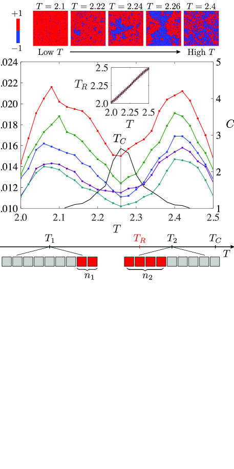
Figure 1: Learning the Ising transition from regression uncertainty. (a) Typical real-space configurations (samples processed directly by the NN) of the ferromagnetic Ising model. (b) Temperature dependence of regression uncertainty $U(T)$ for reconstructing temperatures $T\in[2.0,2.5]$ ($\Delta T=2\times 10^{-2}$) of Ising model with $L=120$ (red curve), $L=140$ (green curve), $L=160$ (blue curve), $L=180$ (purple curve), and $L=200$ (cyan curve). The curve of regression uncertainty $U(T)$ assumes a non-trivial M-shape and the valley appears at $T=2.26\pm 0.01$ which matches the critical temperature $T_{C}=2/\ln(1+\sqrt{2})\approx 2.269$, suggesting that it contains non-trivial information, i.e., the position of the valley, which can be utilized to reveal possible phase transitions. The black curve corresponds to the temperature dependence of the system’s heat capacity $C(T)$ with $L=180$. Inset: Regression results of a well-trained NN for the corresponding ISP with $L=120$. The reconstructed temperature $T_{R}$ is very close to the target $T$ (the diagonal line represents the ideal regression results $T_{R}=T$ for the ISP), but there always exists an intrinsic regression uncertainty $U(T)$ as shown by the error bars and the range of the colored error band. (c) Schematic illustration of the origin of the hidden information in regression uncertainty. In a simple scenario of reconstructing two temperatures $T_{1}$ and $T_{2}$ ($T_{1}<T_{2}<T_{C}$), which involves two sets of an equal number of samples (illustrated by squares) generated probabilistically at $T_{1}$ and $T_{2}$, respectively, there can be $n_{1}$ samples in the set of $T_{1}$ with relatively high energy that are essentially indistinguishable from $n_{2}$ samples in the set of $T_{2}$ with relatively low energy. To deal with these $n_{1}+n_{2}$ indistinguishable samples (illustrated by red squares), a simple but still decent way for the NN to accomplish its regression task is to associate them with their weighted average temperature. As a result, their $T_{R}$ tends to be closer to $T_{2}$ rather than $T_{1}$ due to $n_{2}>n_{1}$ since the heat capacity that characterizes the strength of thermal fluctuations satisfies $C(T_{2})>C(T_{1})$ in this case, which leads to $U(T_{2})<U(T_{1})$. This indicates that the temperature at which $C(T)$ reaches its maximum should match exactly the temperature at which $U(T)$ reaches its minimum as shown in (b). See text for more details.

II.2 Connection between regression uncertainty and response properties

To gain more intuitions for understanding the behavior of regression uncertainty shown in Fig. 1(b) and see the possible origin of its non-trivial information concerning phase transitions, let us consider the training process of the NN in a simple scenario where it is fed with only two sets of an equal number of samples generated at temperatures $T_{1}$ and $T_{2}$ near the critical temperature $T_{C}$ with $T_{1}<T_{2}<T_{C}$. Since the samples [illustrated by squares in Fig. 1(c)] in these two sets are generated probabilistically, one expects that certain amount of samples, say $n_{1}$ samples, that correspond to relatively high energy in the set of $T_{1}$ are essentially indistinguishable from certain amount of samples, say $n_{2}$ samples, that correspond to relatively low energy in the set of $T_{2}$ [illustrated by red squares in Fig. 1(c)]. These essentially indistinguishable samples make it impossible for any algorithm to perform the ISP regression perfectly (corresponding to $\mathbb{L}=0$).

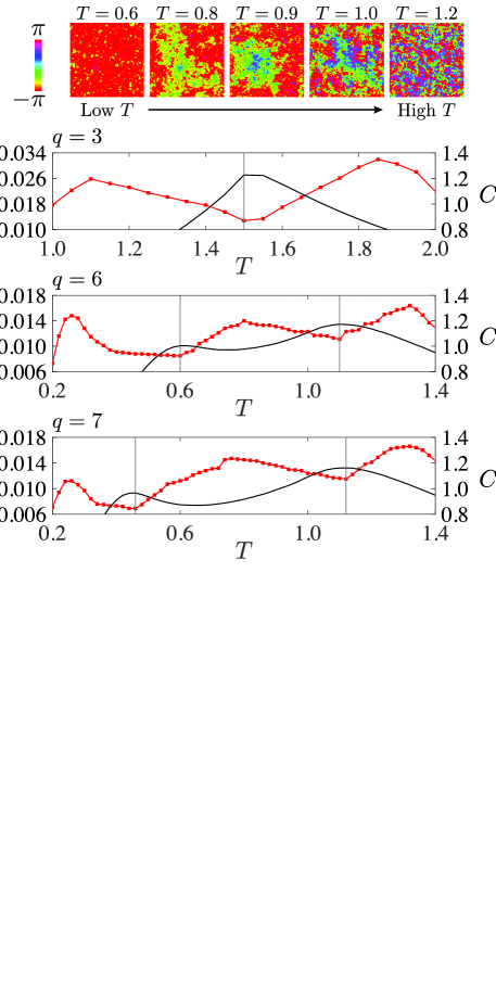
Figure 2: Learning the $q$-state clock model from regression uncertainty. (a) Typical real-space configurations of the six-state clock model for instance. (b) Temperature dependence of regression uncertainty $U(T)$ for reconstructing temperatures $T\in[1,2]$ ($\Delta T=5\times 10^{-2}$) of the three-state clock model with $L=100$. The curve of regression uncertainty $U(T)$ (red curve) also assumes an M-shape and the valley appears at $T=1.500\pm 0.025$ which matches the critical temperature $T_{C}=3/(2\ln(1+\sqrt{3}))\approx 1.492$, suggesting that it also contains non-trivial information, i.e., the position of the valley, which can serve as a generic tool for identifying continuous phase transitions. The black curve corresponds to the temperature dependence of the system’s heat capacity $C(T)$. (c) Temperature dependence of regression uncertainty $U(T)$ for reconstructing temperatures $T\in[0.2,1.4]$ ($\Delta T=2\times 10^{-2}$) of the six-state clock model with $L=100$. The curve of regression uncertainty $U(T)$ (red curve) assumes two successive M-shapes in this case, indicating that the six-state clock model assumes three different phases, i.e., an intermediate phase that is absent in its two-state (Ising) and three-state counterparts. The positions of the two minima of regression uncertainty $U(T)$ correspond to the two maxima of the system’s response function with respect to the temperature, i.e., the heat capacity $C(T)$ (black curve), hence not to the BKT transition points in this system. (d) Analogs of (c), but for the seven-state clock model. See text for more details.

To give a reconstructed temperature $T_{R}$ to these $n_{1}+n_{2}$ indistinguishable samples, one can image that in practice, the NN could adopt some oversimplified and crude ways if it is totally confused, e.g., associating all with $T_{1}$ (or $T_{2}$) without distinction or just randomly guessing. Beyond these bad candidates, a simple but still decent way for the NN to accomplish its regression task is to associate the $n_{1}+n_{2}$ indistinguishable samples with their weighted average temperature $T_{R}=(n_{1}T_{1}+n_{2}T_{2})/(n_{1}+n_{2})$. Indeed, the NN can learn better ways by itself, but if its actual output $T_{R}$ largely departs from this weighted average, one can hardly expect an overall good performance of ISP. Further noticing that in the data generation according to the probability distribution $\exp(-H/T)/Z$, stronger thermal fluctuations make those samples with their energy deviating from the average energy of the set more easily to be accessed, one thus expects $n_{2}>n_{1}$ since thermal fluctuations at $T_{2}$ are stronger than $T_{1}$ for $T_{1}<T_{2}<T_{C}$. Then the weighted average is closer to $T_{2}$ rather than $T_{1}$, so is the reconstructed temperature $T_{R}$. This thus gives rise to a smaller regression uncertainty at $T_{2}$ compared to the one at $T_{1}$, i.e., $U(T_{2})<U(T_{1})$. Similarly, one expects the opposite for the case $T_{C}<T_{1}<T_{2}$, i.e., $U(T_{1})<U(T_{2})$. Moreover, the strength of thermal fluctuations at different temperature $T$ can be characterized by the response property of the system with respect to the temperature, i.e., by the heat capacity $C(T)=(\langle H^{2}\rangle-\langle H\rangle^{2})/(NT^{2})$. This indicates that a larger heat capacity corresponds to a smaller regression uncertainty, and in particular, the temperature at which the heat capacity $C(T)$ reaches its maximum should match exactly the temperature at which the regression uncertainty $U(T)$ reaches its minimum. As shown by the heat capacity curve in Fig. 1(b), the temperature of the peak of $C(T)$ indeed assumes the same value as the one of the valley of $U(T)$. Actually, one can also see in the following that the valley position of regression uncertainty $U(T)$ generally show a consistency with the peak position of heat capacity $C(T)$, not only in the case of the ferromagnetic Ising model, but in the cases of three-, six-, and seven-state clock models as well, supporting the above understanding on the origin of the hidden information in regression uncertainty.

It is worth mentioning that although the connection between $U(T)$ and $C(T)$ discussed above generally hold true, in practical calculations, since the temperature region where the regression is performed is a finite interval, the behavior of $U(T)$ can also be influenced by the boundary effect of the region. This boundary effect in fact gives rises to the maxima of $U(T)$ shown in Fig. 1(b). Consider for instance the regime below $T_{C}$, one observes that as the temperature increases, the regression uncertainty $U(T)$ increases, and reaches a local maximum. The origin of this behavior can be understood by comparing the regression uncertainty at the left boundary of the temperature region ($T=2.0$) with the one at the temperature that is a bit away from the left boundary (e.g., $T=2.02$). $U(T=2.02)$ is larger than $U(T=2.0)$ in this case, since when the NN tries to reconstruct the temperature at $T=2.02$, it is confused by both the similar configurations that appear at $T=2.0$ and the ones that appear at temperatures higher than $T=2.02$, while for reconstructing the temperature at the left boundary $T=2.0$, it is only confused by the similar configurations that appear at temperatures higher than $T=2.0$. As shown in more detailed investigations on this boundary effect presented in Appendix B [see in particular Fig. 4(b)], the maxima of $U(T)$ depend on the choice of the temperature region where the regression is performed, while in sharp contrast, the temperature that corresponds to the non-trivial minimum of $U(T)$ remains invariant at the critical temperature $T_{C}$.

II.3 The generic application of regression uncertainty in learning continuous phase transitions

The above investigations on ISP in the ferromagnetic Ising model reveal an intrinsic connection between regression uncertainty and response properties of the system. By utilizing this connection, a new type of unsupervised machine learning approach LFRU is established in this work for revealing possible phase transitions. To further demonstrate LFRU as a generic tool for identifying continuous phase transitions, let us consider the $q=3$ case of the $q$-state clock model $H_{q}=-J\sum_{\langle i,j\rangle}\cos(\theta_{i}-\theta_{j})$, where $\theta_{i}=2\pi n_{i}/q$ denotes the $q$-valued spin located at the lattice site $i$ with $n_{i}=0,1,\ldots,q-1$. The generic ability of deep NNs in image recognition enables LFRU to be directly applied to this model with no additional design. Actually, the training and testing processes are exactly the same in practice as the ones involved in studying the ferromagnetic Ising model. Here, the NN is trained to perform the ISP regression for reconstructing temperatures $T\in[1,2]$ ($\Delta T=5\times 10^{-2}$) of the three-state clock model, then test its performance and calculate the corresponding regression uncertainty. As one can see from Fig. 2(b), the temperature dependence of regression uncertainty $U(T)$ in this case also assumes an M-shape. In particular, the valley position $T=1.500\pm 0.025$ matches the critical temperature $T_{C}=3/(2\ln(1+\sqrt{3}))\approx 1.492$ (Savit_RMP_1980, ; Wu_RMP_1982, ; Ortiz_NPB_2012, ) of the continuous phase transition point of this system.

Remarkably, although the ISP regression algorithm itself is supervised since there are labels attached to each sample, LFRU can still be regarded as an unsupervised approach since those labels (e.g., temperature $T$, rather than phase A/B) do not provide the NN with any prior physical knowledge about the actual target of LFRU, i.e., possible phase transitions. As already shown concretely in the ferromagnetic Ising model and the three-state clock model, one directly trains the NN to perform regression tasks of the corresponding ISP and then calculates the regression uncertainty of the well-trained NN afterward [see Eq. (2) for instance]. By the non-trivial minimum of regression uncertainty, the key information concerning possible phase transitions is unsupervisedly revealed (see Appendix D for a blank comparison with no phase transition involved). For continuous phase transitions, the corresponding response functions diverge (reach the maximum for finite-size systems) at the critical point, so the position of the non-trivial minimum of regression uncertainty directly corresponds to the critical point of phase transitions [see Figs. 1(b) and 2(b) for instance]. In particular, when applying LFRU, one does not need to calculate the response functions such as the heat capacity, hence LFRU can assume practical advantages over conventional approaches in revealing possible phase transitions of the systems where directly calculating the heat capacity or other relevant observables is highly non-trivial or even impossible, e.g., fermion or spin systems with sign problems (Khatami_PRX_2017, ; Broecker_Sci_Rep_2017, ; Loh_PRB_1990_SignProblem, ). Moreover, noticing that LFRU does not assume the number of existing phases in the system under consideration, one could directly use it to investigate complex physical systems with possible intermediate phases (Loerting_RMP_2016_water, ; Digregorio_PRL_2018, ; Ciamarra_PRL_2020, ; Zhu_Zheng_PRB_2021, ; Tianxing_Ma_PRB_2020, ; Fontenele_PRL_2019, ). As one shall see in the concrete example presented in the following, LFRU can indeed reveal the key information concerning intermediate phases.

III Reveal intermediate phases from regression uncertainty

Let us now discuss how phase transitions in systems with possible intermediate phases can be investigated by LFRU. To this end, here the $q=6,7$ cases of the $q$-state clock model are focused for instance. These models exhibit an intermediate vortex-antivortex condensed BKT phase between paramagnetic and ferromagnetic phases (Kosterlitz_Rep_Prog_Phys_2016, ; Kosterlitz_JPhysC_1973, ; Kosterlitz_JPhysC_1974, ), hence in recent years are typically employed to examine the ability of new machine learning approaches (Miyajima_PRB_2021, ; Lee_PRE_2019, ; Scheurer_Nat_Phys_2019, ; Scheurer_PRL_2020, ; Jiang_PRB_2020, ; Wei_PRE_2019, ).

To investigate the temperature-driven phase transitions in the six-state and seven-state clock models, we first train the NN to perform the ISP regression for reconstructing the temperature $T$ in these two models, and then calculate their respective regression uncertainty. As one can see from the temperature dependence of regression uncertainty $U(T)$ shown in Fig. 2(c) and Fig. 2(d), both the $U(T)$ curves assume two successive M-shapes. Such a structure with two non-trivial minima, instead of one, is in sharp contrast to the ones presented in Fig. 1 and Fig. 2(b), indicating that the six-state and seven-state clock models assume three different phases, i.e., an intermediate phase that is absent in their two-state (Ising) and three-state counterparts. This thus provides a new type of data-driven evidence on the existence of the intermediate phase in these two models, corroborating the results in previous investigations employing conventional approaches such as the ones utilizing the helicity modulus (Kumano_PRB_2013, ; Baek_PRE_2013, ), the Fisher zeros (Hwang_PRE_2009, ; Hong_PRE_2020, ), the entanglement entropy of the fixed-point matrix-product-state (Ziqian_Li_PRE_2020, ), etc.

At this stage one may incline to associate the two minima of regression uncertainty $U(T)$ shown in Fig. 2(c) or Fig. 2(d) with the two transition points of the six-state or seven-state clock model. But thanks to the physical interpretability of LFRU’s outputs, it is clear that the two minima of regression uncertainty $U(T)$ should correspond to the two maxima of the system’s response function with respect to $T$, i.e., the heat capacity $C(T)$, which is indeed the case as shown by the vertical lines in Figs. 2(c) and 2(d). Noticing that the phase transitions associated with the intermediate phase in these two models are of the BKT type, i.e., driven by topological defects (Ziqian_Li_PRE_2020, ; Hostetler_PRD_2021, ), the positions of the two maxima of heat capacity $C(T)$ in fact do not exactly match the critical temperatures (Ziqian_Li_PRE_2020, ; Hostetler_PRD_2021, ), indicating that the positions of the two minima of regression uncertainty $U(T)$ in Figs. 2(c) and 2(d) should not be interpreted as the BKT transition points. This on the one hand clarifies that quantitatively identifying critical points via LFRU is restricted to continuous phase transitions, and on the other hand provides data-driven evidence that the transitions in these systems are not of the Landau type, corroborating recent investigations (Hong_PRE_2020, ; Ziqian_Li_PRE_2020, ; Hostetler_PRD_2021, ; Miyajima_PRB_2021, ).

Finally, another remarkable aspect of LFRU’s implementation to highlight is the robustness against different choices of the NN architecture. All the machine learning results presented in Fig. 1 and Fig. 2 are obtained by employing a widely-used NN that is known as ResNet (Kaiming_He_IEEE_CVPR_2016, ). In Appendix A, the same analysis is performed employing another type of widely-used NN that is known as GoogLeNet (Szegedy_IEEE_CVPR_2015, ). Their corresponding results agree very well with each other, suggesting that state-of-the-art developments in the field of artificial intelligence and data science can be readily exploited to automatically detect phases of matter in a physically interpretable manner via LFRU.

IV Conclusions

The ISP usually has a primary focus on accurately and precisely inferring system parameters, and thus the uncertainty of regression results was naturally considered as unfavorable for performing such regression tasks. However, this unfavorable regression uncertainty actually assumes an intrinsic connection to the system’s response properties, making it accommodate crucial information concerning possible phase transitions of the system under consideration. This enables the development of a fundamentally new type of generic unsupervised machine learning approach LFRU for automated detection of phases of matter, which is based on regression instead of classification and produces physically interpretable results, as manifested concretely in the cases of Ising model and the three-, six-, and seven-state clock models. The working mechanism of this approach is quite general, so its application is not restricted to temperature-driven transitions investigated here. Moreover, noticing that NNs can easily deal with not only the data generated from numerical simulations but also experimental data (Rem_Nat_Phys_2019, ), including both the real optical imaging (Mulimani_PRR_2020, ) and preprocessed physical configurations such as snapshots of the many-body density matrix (Bohrdt_Nat_Phys_2019, ), hence LFRU is expected to be available for analyzing actual experiments as well. In addition, various possible phase transitions in a wide range of nonequilibrium complex many-body systems (Volpe_Nat_Mach_Intell_2020, ; Chate_Annu_Rev_2020, ; Munoz_RMP_2018, ; Volpe_RMP_2016, ; Vicsek_Phys_Rep_2012, ), such as the active matter systems described by the Vicsek model (Vicsek_PRL_1995, ) consisting of self-propelled particles, can likewise be investigated via this approach (Footnote, ). In these regards, we believe that our findings will stimulate further efforts in both developing and applying physically interpretable machine learning approaches to unveil new physics in both equilibrium and nonequilibrium complex many-body systems.

Appendix A Data generation and NN training

In this work, the data generation for the ferromagnetic Ising model is done by Monte Carlo simulations using the Swendsen-Wang algorithm (Swendsen_Wang_PRL_1987, ; Swendsen_Wang_PhysA_1990, ) on the Ising Hamiltonian $H$ with periodic boundary condition imposed. For the ferromagnetic Ising model with each system size $L=120,140,160,180,200$, there are $7\times 10^{3}$ samples of the steady state spin configuration generated at each temperature $T$ in the temperature region $[2.0,2.5]$ with the temperature spacing kept as $\Delta T=2\times 10^{-2}$, and in the temperature region $[2.25,2.30]$ with $\Delta T=2\times 10^{-3}$, respectively. These samples are converted to images as shown in Fig. 1(a), where the blue or red at each pixel represents the spin $s_{i}$ on the $i$th lattice site, and then divided into three categories in the ratio of 5:1:1 forming the training, validation, and test datasets (Goodfellow_Book_2016, ). The data generation for the $q$-state clock model is done by Monte Carlo simulations on the Hamiltonian $H_{q}$ with periodic boundary condition imposed. For $q=3$ with $L=100$, there are $7\times 10^{3}$ samples of the steady state spin configuration generated at each temperature $T$ in the temperature region $[1,2]$ with $\Delta T=5\times 10^{-2}$. For $q=6,7$ with $L=100$, there are $7\times 10^{3}$ samples of the steady state spin configuration generated at each temperature $T$ in the temperature region $[0.2,1.4]$ with $\Delta T=2\times 10^{-2}$, respectively. These samples are also converted to images as shown in Fig. 2(a), where the cyclic color at each pixel represents the planar angle $\theta_{i}$ on the $i$th lattice site, and then divided into three categories in the same ratio as above forming the datasets.

Using these datasets, two widely-used NNs are employed, namely, ResNet (Kaiming_He_IEEE_CVPR_2016, ) and GoogLeNet (Szegedy_IEEE_CVPR_2015, ), to perform regression tasks of ISP. The results obtained by ResNet are shown in Fig. 1 and Fig. 2 in the main text, and the results obtained by GoogLeNet are shown in Fig. 3. These NNs are similarly trained by using the Adam optimizer (Kingma_ICLR_2015, ) traversing the training dataset for 10 epochs at a learning rate $\alpha=10^{-3}$, together with a validation at each epoch traversing the validation dataset. After that, the samples in the test datasets are used to calculate the regression uncertainty $U(T)$. All the machine learning results in this work are averaged over 20 independent training and testing processes.

Appendix B Loss function, and the maxima of regression uncertainty

In the main text, the mean square error (MSE) loss function $\mathbb{L}=\langle(T-T_{R})^{2}\rangle$ is employed to train the NN for instance. Here, for the sake of completeness, the same analysis is performed employing the mean absolute error (MAE) loss function $\mathbb{L}=\langle|T-T_{R}|\rangle$, which is another widely-used loss function that is suitable for regression tasks. Their results are presented in Fig. 4(a). For reconstructing temperatures $T\in[2.0,2.5]$ ($\Delta T=2\times 10^{-2}$) of Ising model with $L=120$, these two different choices of loss function give rise to similar behavior of regression uncertainty. In particular, the corresponding valley positions of regression uncertainty $U(T)$ are numerically the same. This thus indicates that the signals generated by LFRU concerning possible phase transitions are robust against different choices of the loss function, as long as the NN trained with the loss function can achieve a good performance in reconstructing the system parameter.

Moreover, to better understand the origin of the maxima of regression uncertainty, the boundary effect of the parameter region where the regression is performed is investigated. It can be seen clearly from Fig. 4(b) by comparing the behaviors of regression uncertainty $U(T)$ for respectively reconstructing temperatures $T\in[2.00,2.40]$, $T\in[2.00,2.46]$, $T\in[2.04,2.50]$, $T\in[2.10,2.50]$ of Ising model. Although the valley of $U(T)$ in these cases remains invariant at the critical temperature $T_{C}$, the hills of $U(T)$ are indeed sensitive to such slight changes of the temperature region, hence their corresponding temperatures do not assume a particular physical significance.

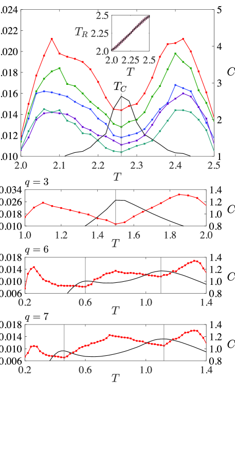
Figure 3: Analogs of Fig. 1(b) and Figs. 2(b-d), but obtained by employing GoogLeNet instead of ResNet. These two employed NNs have very different designs for the feature extraction, but their results match very well, manifesting that the implementation of LFRU is robust against different choices of the NN architecture. See text for more details.

Appendix C Finite-size analysis

Temperatures $T\in[2.0,2.5]$ ($\Delta T=2\times 10^{-2}$) of Ising model are reconstructed in Fig. 1(b) in the main text. Here, a detailed check in the vicinity of $T_{C}$ with a higher resolution is performed. As one can see from Fig. 5(a), for reconstructing temperatures $T\in[2.25,2.30]$ with $\Delta T=2\times 10^{-3}$, the temperature dependence of regression uncertainty $U(T)$ also assumes the M-shape. According to its valley, the predicted critical temperature $T_{C}(L)$ for each system size is $T_{C}(L=120)=2.278\pm 0.001$, $T_{C}(L=140,160,180)=2.276\pm 0.001$, $T_{C}(L=200)=2.274\pm 0.001$. The maximum position of $C(T)$ shown in Fig. 5(b) shifts among different system sizes due to finite-size effects, but the intrinsic connection between regression uncertainty and response properties ensures that the position of the valley of $U(T)$ in Fig. 5(a) keeps matching the maximum position of $C(T)$ irrespective of the system size. These finite-size data of $T_{C}(L)$ are fitted as a function of $1/L$ as shown in the inset of Fig. 5(a), which leads to an estimation of $T_{C}=2.270\pm 0.001$ (the resolution is determined by $\Delta T$) for the critical temperature in the thermodynamic limit.

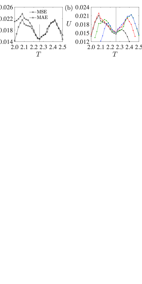
Figure 4: (a) Temperature dependence of regression uncertainty $U(T)$ for reconstructing temperatures $T\in[2.0,2.5]$ ($\Delta T=2\times 10^{-2}$) of Ising model with $L=120$ obtained by using the mean square error (MSE) and the mean absolute error (MAE) loss functions to train ResNet, respectively. Their valley positions of regression uncertainty $U(T)$ are numerically the same, suggesting that LFRU’s implementation is robust against different reasonable choices of the loss function. (b) Temperature dependence of regression uncertainty $U(T)$ for reconstructing temperatures $T\in[2.00,2.40]$ (corresponding to the black curve), $T\in[2.00,2.46]$ (red), $T\in[2.04,2.50]$ (green), and $T\in[2.10,2.50]$ (blue), respectively, of Ising model with $L=120$, $\Delta T=2\times 10^{-2}$. Maxima of regression uncertainty $U(T)$ depend on the choice of the temperature region where the regression is performed, while in sharp contrast, the temperature that corresponds to the non-trivial minimum of $U(T)$ remains invariant at $T=2.26\pm 0.01$. These results suggest that the boundary effect of the parameter region only imposes noticeable influences on the maxima positions of regression uncertainty, while as long as there exists at least two phases in the parameter region where the regression is performed, the LFRU’s implementation and the valley positions of regression uncertainty, i.e., the critical point predicted via LFRU, are robust against different reasonable choices of the parameter region. See text for more details.

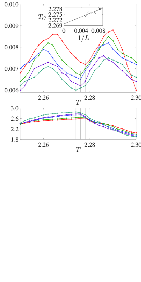
Figure 5: (a) Temperature dependence of regression uncertainty $U(T)$ for reconstructing temperatures $T\in[2.25,2.30]$ ($\Delta T=2\times 10^{-3}$) of Ising model with $L=120$ (red curve), $L=140$ (green), $L=160$ (blue), $L=180$ (purple), and $L=200$ (cyan). The valley of $U(T)$ appears at $T=2.278\pm 0.001$ for $L=120$, at $T=2.276\pm 0.001$ for $L=140,160,180$, at $T=2.274\pm 0.001$ for $L=200$. Inset: Fitting of valley position $T_{C}(L)$ of regression uncertainty $U(T)$ as a function of $1/L$, which leads to an estimation of $T_{C}=2.270\pm 0.001$ for the critical temperature in the thermodynamic limit. (b) System’s heat capacity $C(T)$ within $[2.25,2.30]$ ($\Delta T=2\times 10^{-3}$) with different system sizes. These results indicate that LFRU is applicable for both the extensive search for phase transitions within a relatively large parameter ranges (corresponding to relatively large $\Delta T$), as well as for the quantitative analysis within the vicinity of critical points (corresponding to relatively small $\Delta T$). See text for more details.

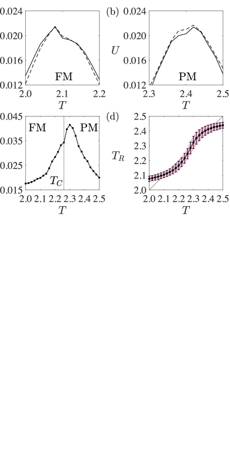
Figure 6: (a) Temperature dependence of regression uncertainty $U(T)$ for reconstructing temperatures $T\in[2.0,2.2]$ ($\Delta T=2\times 10^{-2}$) of Ising model with $L=120$. Only the ferromagnetic (FM) phase exists in this temperature region, so the curve of $U(T)$ assumes no non-trivial minimum. The solid curve and the dashed curve represent the results obtained by ResNet and GoogLeNet, respectively. (b) Analogs of (a), but concerning the high-temperature region $[2.3,2.5]$ where only the paramagnetic (PM) phase exists. These results confirm that LFRU does not require prior system-specific knowledge about the number of existing phases as a given condition. (c) Temperature dependence of regression uncertainty $U(T)$ for reconstructing temperatures $T\in[2.0,2.5]$ ($\Delta T=2\times 10^{-2}$) of Ising model with $L=120$ obtained by using a very simple fully-connected NN that assumes a deliberately produced poor performance on ISP. This curve of $U(T)$ looks similar to the ones presented in (a) and (b) with no phase transition involved, suggesting that the NN’s good performance on ISP is a prerequisite of LFRU for automated detection of phases of matter. (d) Regression results corresponding to (c). The reconstructed temperature $T_{R}$ largely departs from the target $T$ (the diagonal line represents the ideal regression results $T_{R}=T$ for the ISP). The error bars and the range of the colored error band represent the regression uncertainty $U(T)$, but here the regression uncertainty no longer contain hidden information that can be utilized to reveal possible phase transitions, since this NN fails to accomplish its regression task. See text for more details.

Appendix D Blank comparison and the performance on ISP

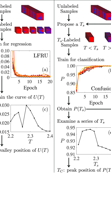
Figure 7: Comparison of LFRU and the learning-by-confusion approach. Left panel: Illustration of applying LFRU for identifying $T_{C}$ of the ferromagnetic Ising model $(L=120)$ with samples generated at $T\in[2.2,2.4]$ with $\Delta T=2\times 10^{-2}$. Right panel: Illustration of applying the learning-by-confusion approach for identifying the same $T_{C}$ with the same datasets. (a) The training process of the NN for reconstructing temperatures, traversing the training dataset for $20$ epochs. Different colors represent different independent trajectories of training. (b) The training process of the NN for classifying phase A ($T<T_{s}$) and phase B ($T>T_{s}$), traversing the same dataset for $20$ epochs. These results show that comparing the implementation of LFRU and the learning-by-confusion approach, they require similar numbers of epochs to give birth to a well-trained NN. (c) Temperature dependence of regression uncertainty $U(T)$ obtained from the well-trained NNs in (a), averaged over $10$ independent trajectories. (d) $T_{s}$ dependence of the classification accuracy $P(T_{s})$ obtained from the well-trained NNs in (b), averaged over $10$ independent trajectories. See text for more details.

For a blank comparison, LFRU is applied here on the ferromagnetic Ising model concerning solely the low-temperature region $[2.0,2.2]$ ($\Delta T=2\times 10^{-2}$) employing both ResNet (Kaiming_He_IEEE_CVPR_2016, ) and GoogLeNet (Szegedy_IEEE_CVPR_2015, ), respectively. As one can see in Fig. 6(a), the temperature dependence of regression uncertainty $U(T)$ assumes a single maximum and no non-trivial minimum, namely, only the boundary effect of the parameter region exhibits signs. This is consistent with the fact that only one phase, i.e., the ferromagnetic phase, exists with no phase transition in the temperature region $[2.0,2.2]$. Similar results are obtained concerning solely the high-temperature region $[2.3,2.5]$ ($\Delta T=2\times 10^{-2}$) that corresponds to only the paramagnetic phase, as shown in Fig. 6(b). These results verify that the non-trivial minimum of regression uncertainty in performing regression tasks of ISP is indeed an unsupervised signal for revealing possible phase transitions of the system under consideration.

It is also worth mentioning that the signals generated by LFRU concerning possible phase transitions are based on the NN’s good performance on ISP. Such a performance is not guaranteed by an arbitrary NN. Here, a poor performance is deliberately produced [see Fig. 6(d)] concerning the temperature region $[2.0,2.5]$ ($\Delta T=2\times 10^{-2}$) on the ferromagnetic Ising model with $L=120$. This is obtained by using a very simple fully-connected NN, which consists of an input layer with $3L^{2}$ neurons (3 for RGB), a hidden layer with $L$ neurons (rectified linear unit as the activation function, batch normalization applied) (Goodfellow_Book_2016, ), and an output layer with only one neuron. It is worth mentioning that the fully-connected NN might also perform well after fine-tuning, but a poor performance is needed here for technical discussions. As one can see from Fig. 6(c), when the NN cannot well accomplish its regression task of ISP, the resulting behavior of regression uncertainty $U(T)$ looks similar to the ones presented in Figs. 6(a) and 6(b) with no phase transition involved. However, the temperature region under consideration in Fig. 6(c) is indeed across $T_{C}$, suggesting that one cannot distinguish whether a single peak of $U(T)$ is associated with a phase transition or not merely by monitoring the regression uncertainty $U(T)$ itself. A reasonable judgment is that any investigation according to the information extracted from a poor performance will suffer from a lack of legitimacy. Therefore, the NN’s good performance on ISP is a prerequisite of LFRU for automated detection of phases of matter.

Appendix E Comparison with the learning-by-confusion approach

Here in this appendix, LFRU is directly compared with the learning-by-confusion approach (van_Nieuwenburg_Nat_Phys_2017, ), which is also an unsupervised learning approach for automated detection of phases of matter. As a concrete example, let us consider identifying $T_{C}$ of the ferromagnetic Ising model with samples generated at temperatures $T\in[2.2,2.4]$ with the temperature spacing $\Delta T=2\times 10^{-2}$. As illustrated in the right panel of Fig. 7, when applying the learning-by-confusion approach, one shall first propose a possible critical point $T_{s}$. After that, the samples satisfying $T<T_{s}$ are accordingly labeled with $(\tilde{y}_{A}=1,\tilde{y}_{B}=0)$ as phase A, and the samples satisfying $T>T_{s}$ are labeled with $(\tilde{y}_{A}=0,\tilde{y}_{B}=1)$ as phase B. Then the NN is trained to perform an NN-based binary classification between these artificial phases, outputting for each sample its confidences $(y_{A},y_{B})$ of identifying the sample as phase A or B. The loss function should be suitable for the binary classification task, e.g., the cross-entropy function $\mathbb{L}^{\prime}=\langle-\tilde{y}_{A}\ln y_{A}-\tilde{y}_{B}\ln y_{B}\rangle$ (Goodfellow_Book_2016, ), instead of the MSE or MAE loss function for regression. After training, one obtains the classification accuracy $P(T_{s})$ that the NN successfully matches the samples in the test dataset with their attached labels corresponding to the proposed $T_{s}$. According to Ref. (van_Nieuwenburg_Nat_Phys_2017, ), one shall examine a series of different $T_{s}$, and the position of the maximum of $P(T_{s})$ is considered the critical point $T_{C}$ predicted via the learning-by-confusion approach. Similar to LFRU, the resolution of $T_{C}$ predicted via the learning-by-confusion approach is also determined by $\Delta T$. The NN used by the learning-by-confusion approach and the NN used by LFRU only have slight differences in their output layers, i.e., there are two neurons in the former for binary classification, but only one single neuron in the latter for regression, and hence the time it takes to train these NNs traversing the same datasets for an epoch is approximately the same. Figs. 7(a) and (b) show that the convergence speed is also similar, so they require similar numbers of epochs to give birth to a well-trained NN. However, a well-trained NN for the learning-by-confusion approach can just give a single $P(T_{s})$, and if there are $m$ different possible values of $T_{s}$ to be examined as $T_{C}$ (at least $m\geqslant 3$, and usually much larger), it requires $m$ well-trained NNs. In sharp contrast, when applying LFRU, a complete curve of $U(T)$ is directly obtained from one well-trained NN, and the valley position of $U(T)$ can be considered as the critical point $T_{C}$ predicted via LFRU. Therefore, the approach developed in this work could be about $m$ times faster than the widely-used learning-by-confusion approach. The direct comparison of their results is presented in Figs. 7(c) and (d).

References

- (1) G. Carleo, I. Cirac, K. Cranmer, L. Daudet, M. Schuld, N. Tishby, L. Vogt-Maranto, and L. Zdeborová, Rev. Mod. Phys. 91, 045002 (2019).
- (2) J. Carrasquilla, Adv. Phys. X 5, 1797528 (2020).
- (3) F. Cichos, K. Gustavsson, B. Mehlig, and G. Volpe, Nat. Mach. Intell. 2, 94 (2020).
- (4) S. J. Wetzel, Phys. Rev. E 96, 022140 (2017).
- (5) L. Wang, Y. Jiang, L. He, and K. Zhou, Chin. Phys. Lett. 39, 120502 (2022).
- (6) L. Wang, Y. Jiang, and K. Zhou, arXiv:2007.01037.
- (7) F. D’Angelo and L. Böttcher, Phys. Rev. Res. 2, 023266 (2020).
- (8) J. Singh, M. Scheurer, and V. Arora, SciPost Phys. 11, 043 (2021).
- (9) J. Carrasquilla and R. G. Melko, Nat. Phys. 13, 431 (2017).
- (10) E. P. L. van Nieuwenburg, Y.-H. Liu, and S. D. Huber, Nat. Phys. 13, 435 (2017).
- (11) J. Venderley, V. Khemani, and E.-A. Kim, Phys. Rev. Lett. 120, 257204 (2018).
- (12) W.-C. Guo, B.-Q. Ai, and L. He, Phys. Rev. E 104, 044611 (2021).
- (13) M. J. S. Beach, A. Golubeva, and R. G. Melko, Phys. Rev. B 97, 045207 (2018).
- (14) P. Suchsland and S. Wessel, Phys. Rev. B 97, 174435 (2018).
- (15) S. S. Lee and B. J. Kim, Phys. Rev. E 99, 043308 (2019).
- (16) M. N. Chernodub, H. Erbin, V. A. Goy, and A. V. Molochkov, Phys. Rev. D 102, 054501 (2020).
- (17) F. Schindler, N. Regnault, and T. Neupert, Phys. Rev. B 95, 245134 (2017).
- (18) Y.-T. Hsu, X. Li, D.-L. Deng, and S. Das Sarma, Phys. Rev. Lett. 121, 245701 (2018).
- (19) K. Ch’ng, J. Carrasquilla, R. G. Melko, and E. Khatami, Phys. Rev. X 7, 031038 (2017).
- (20) P. Broecker, J. Carrasquilla, R. G. Melko, and S. Trebst, Sci. Rep. 7, 8823 (2017).
- (21) I. Goodfellow, Y. Bengio, and A. Courville, Deep Learning (MIT Press, Cambridge, 2016).
- (22) S.-M. Udrescu and M. Tegmark, Sci. Adv. 6, eaay2631 (2020).
- (23) T. Wu and M. Tegmark, Phys. Rev. E 100, 033311 (2019).
- (24) Z. Liu, B. Wang, Q. Meng, W. Chen, M. Tegmark, and T.-Y. Liu, Phys. Rev. E 104, 055302 (2021).
- (25) S.-M. Udrescu and M. Tegmark, Phys. Rev. E 103, 043307 (2021).
- (26) Z. Liu and M. Tegmark, Phys. Rev. Lett. 128, 180201 (2022).
- (27) Z. Liu and M. Tegmark, Phys. Rev. Lett. 126, 180604 (2021).
- (28) F. Schäfer and N. Lörch, Phys. Rev. E 99, 062107 (2019).
- (29) E. Greplova, A. Valenti, G. Boschung, F. Schäfer, N. Lörch, and S. D. Huber, New J. Phys. 22, 045003 (2020).
- (30) J. Arnold, F. Schäfer, M. Žonda, and A. U. J. Lode, Phys. Rev. Res. 3, 033052 (2021).
- (31) J. Arnold and F. Schäfer, Phys. Rev. X 12, 031044 (2022).
- (32) D. E. Gökmen, Z. Ringel, S. D. Huber, and M. Koch-Janusz, Phys. Rev. Lett. 127, 240603 (2021).
- (33) D. E. Gökmen, Z. Ringel, S. D. Huber, and M. Koch-Janusz, Phys. Rev. E 104, 064106 (2021).
- (34) W. Zhang, L. Wang, and Z. Wang, Phys. Rev. B 99, 054208 (2019).
- (35) S.-H. Li and L. Wang, Phys. Rev. Lett. 121, 260601 (2018).
- (36) H.-Y. Hu, S.-H. Li, L. Wang, and Y.-Z. You, Phys. Rev. Res. 2, 023369 (2020).
- (37) C. Miles, A. Bohrdt, R. Wu, C. Chiu, M. Xu, G. Ji, M. Greiner, K. Q. Weinberger, E. Demler, and E.-A. Kim, Nat. Commun. 12, 3905 (2021).
- (38) C. Miles, R. Samajdar, S. Ebadi, T. T. Wang, H. Pichler, S. Sachdev, M. D. Lukin, M. Greiner, K. Q. Weinberger, and E.-A. Kim, arXiv:2112.10789.
- (39) W.-C. Guo, B.-Q. Ai, and L. He, Europhys. Lett. 136, 48002 (2021).
- (40) H. C. Nguyen, R. Zecchina, and J. Berg, Adv. Phys. 66, 197 (2017).
- (41) E. Aurell and M. Ekeberg, Phys. Rev. Lett. 108, 090201 (2012).
- (42) H. C. Nguyen and J. Berg, Phys. Rev. Lett. 109, 050602 (2012).
- (43) A. Decelle and F. Ricci-Tersenghi, Phys. Rev. E 94, 012112 (2016).
- (44) C. Donner and M. Opper, Phys. Rev. E 96, 062104 (2017).
- (45) J. Jo, D.-T. Hoang, and V. Periwal, Phys. Rev. E 101, 032107 (2020).
- (46) D. Wu, L. Wang, and P. Zhang, Phys. Rev. Lett. 122, 080602 (2019).
- (47) P. Contucci, R. Luzi, and C. Vernia, J. Phys. A: Math. Theor. 50, 205002 (2017).
- (48) S. V. Beentjes and A. Khamseh, Phys. Rev. E 102, 053314 (2020).
- (49) R. Fournier, L. Wang, O. V. Yazyev, and Q. Wu, Phys. Rev. Lett. 124, 056401 (2020).
- (50) G. J. Percebois and D. Weinmann, Phys. Rev. B 104, 075422 (2021).
- (51) J. B. Kogut, Rev. Mod. Phys. 51, 659 (1979).
- (52) J. M. Kosterlitz, Rep. Prog. Phys. 79, 026001 (2016).
- (53) J. M. Kosterlitz and D. J. Thouless, J. Phys. C 6, 1181 (1973).
- (54) J. M. Kosterlitz, J. Phys. C 7, 1046 (1974).
- (55) X.-Y. Dong, F. Pollmann, and X.-F. Zhang, Phys. Rev. B 99, 121104 (2019).
- (56) R. Zhang, B. Wei, D. Zhang, J.-J. Zhu, and K. Chang, Phys. Rev. B 99, 094427 (2019).
- (57) A. Canabarro, F. F. Fanchini, A. L. Malvezzi, R. Pereira, and R. Chaves, Phys. Rev. B 100, 045129 (2019).
- (58) M. Jo, J. Lee, K. Choi, and B. Kahng, Phys. Rev. Res. 3, 013238 (2021).
- (59) R. Savit, Rev. Mod. Phys. 52, 453 (1980).
- (60) F. Y. Wu, Rev. Mod. Phys. 54, 235 (1982).
- (61) G. Ortiz, E. Cobanera, and Z. Nussinov, Nucl. Phys. B 854, 780 (2012).
- (62) E. Y. Loh, J. E. Gubernatis, R. T. Scalettar, S. R. White, D. J. Scalapino, and R. L. Sugar, Phys. Rev. B 41, 9301 (1990).
- (63) K. Amann-Winkel, R. Böhmer, F. Fujara, C. Gainaru, B. Geil, and T. Loerting, Rev. Mod. Phys. 88, 011002 (2016).
- (64) P. Digregorio, D. Levis, A. Suma, L. F. Cugliandolo, G. Gonnella, and I. Pagonabarraga, Phys. Rev. Lett. 121, 098003 (2018).
- (65) Y.-W. Li and M. P. Ciamarra, Phys. Rev. Lett. 124, 218002 (2020).
- (66) R.-Y. Sun and Z. Zhu, Phys. Rev. B 104, L121118 (2021).
- (67) J. Wang, L. Zhang, R. Ma, Q. Chen, Y. Liang, and T. Ma, Phys. Rev. B 101, 245161 (2020).
- (68) A. J. Fontenele, N. A. P. de Vasconcelos, T. Feliciano, L. A. A. Aguiar, C. Soares-Cunha, B. Coimbra, L. Dalla Porta, S. Ribeiro, A. J. a. Rodrigues, N. Sousa, P. V. Carelli, and M. Copelli, Phys. Rev. Lett. 122, 208101 (2019).
- (69) Y. Miyajima, Y. Murata, Y. Tanaka, and M. Mochizuki, Phys. Rev. B 104, 075114 (2021).
- (70) J. F. Rodriguez-Nieva and M. S. Scheurer, Nat. Phys. 15, 790 (2019).
- (71) M. S. Scheurer and R. J. Slager, Phys. Rev. Lett. 124, 226401 (2020).
- (72) D. R. Tan and F. J. Jiang, Phys. Rev. B 102, 224434 (2020).
- (73) W. Zhang, J. Liu, and T. C. Wei, Phys. Rev. E 99, 032142 (2019).
- (74) Y. Kumano, K. Hukushima, Y. Tomita, and M. Oshikawa, Phys. Rev. B 88, 104427 (2013).
- (75) S. K. Baek, H. Mäkelä, P. Minnhagen, and B. J. Kim, Phys. Rev. E 88, 012125 (2013).
- (76) C. O. Hwang, Phys. Rev. E 80, 042103 (2009).
- (77) S. Hong and D. H. Kim, Phys. Rev. E 101, 012124 (2020).
- (78) Z.-Q. Li, L.-P. Yang, Z. Y. Xie, H.-H. Tu, H.-J. Liao, and T. Xiang, Phys. Rev. E 101, 060105 (2020).
- (79) L. Hostetler, J. Zhang, R. Sakai, J. Unmuth-Yockey, A. Bazavov, and Y. Meurice, Phys. Rev. D 104, 054505 (2021).
- (80) K. He, X. Zhang, S. Ren, and J. Sun, in Proceedings of the 2016 IEEE Conference on Computer Vision and Pattern Recognition (IEEE CVPR, Las Vegas, 2016) pp. 770–778.
- (81) C. Szegedy, W. Liu, Y. Jia, P. Sermanet, S. Reed, D. Anguelov, D. Erhan, V. Vanhoucke, and A. Rabinovich, in Proceedings of the 2015 IEEE Conference on Computer Vision and Pattern Recognition (IEEE CVPR, Boston, 2015) pp. 1–9.
- (82) B. S. Rem, N. Käming, M. Tarnowski, L. Asteria, N. Fläschner, C. Becker, K. Sengstock, and C. Weitenberg, Nat. Phys. 15, 917 (2019).
- (83) M. K. Mulimani, J. K. Alageshan, and R. Pandit, Phys. Rev. Res. 2, 023155 (2020).
- (84) A. Bohrdt, C. S. Chiu, G. Ji, M. Xu, D. Greif, M. Greiner, E. Demler, F. Grusdt, and M. Knap, Nat. Phys. 15, 921 (2019).
- (85) H. Chaté, Annu. Rev. Condens. Matter Phys. 11, 189 (2020).
- (86) M. A. Muñoz, Rev. Mod. Phys. 90, 031001 (2018).
- (87) C. Bechinger, R. Di Leonardo, H. Löwen, C. Reichhardt, G. Volpe, and G. Volpe, Rev. Mod. Phys. 88, 045006 (2016).
- (88) T. Vicsek and A. Zafeiris, Phys. Rep. 517, 71 (2012).
- (89) T. Vicsek, A. Czirók, E. Ben-Jacob, I. Cohen, and O. Shochet, Phys. Rev. Lett. 75, 1226 (1995).
- (90) In our new work (Guo_Acta_2023, ), clues have been found that the noise strength dependence of the regression uncertainty for reconstructing of the Vicsek model also assumes an M-shape and the valley position matches well with the critical point of this nonequilibrium active matter system.
- (91) R. H. Swendsen and J.-S. Wang, Phys. Rev. Lett. 58, 86 (1987).
- (92) J.-S. Wang and R. H. Swendsen, Phys. A: Stat. Mech. Appl. 167, 565 (1990).
- (93) D. P. Kingma and J. Ba, arXiv:1412.6980.
- (94) W.-C. Guo, B.-Q. Ai, and L. He, Acta Phys. Sin. 72, 200701 (2023).