Simulating neutron star mergers with the Lagrangian Numerical Relativity code SPHINCS_BSSN

Abstract

We present the first neutron star merger simulations performed with the newly developed Numerical Relativity code SPHINCS_BSSN. This code evolves the spacetime on a mesh using the BSSN formulation, but matter is evolved via Lagrangian particles according to a high-accuracy version of general-relativistic Smooth Particle Hydrodynamics (SPH). Our code contains a number of new methodological elements compared to other Numerical Relativity codes. The main focus here is on the new elements that were introduced to model neutron star mergers. These include a) a refinement (fixed in time) of the spacetime-mesh, b) corresponding changes in the particle–mesh mapping algorithm and c) a novel way to construct SPH initial data for binary systems via the recently developed “Artificial Pressure Method.” This latter method makes use of the spectral initial data produced by the library LORENE, and is implemented in a new code called SPHINCS_ID. While our main focus is on introducing these new methodological elements and documenting the current status of SPHINCS_BSSN, we also show as a first application a set of neutron star merger simulations employing “soft” ($\Gamma=2.00$) and “stiff” ($\Gamma=2.75$) polytropic equations of state.

1 Introduction

With the first observation of a merging binary black hole in 2015 abbott16a , gravitational wave detections have become an active part of observational astronomy. The first detection of a merging neutron star binary abbott17a ; abbott17b ; abbott17c ; abbott17d ; smartt17 ; tanaka17 ; villar17 , in both gravitational waves (GWs) and electromagnetic (EM) radiation, followed in 2017 and this watershed event (hereafter referred to as GW170817) settled many long-standing open questions. It showed, among other things, that neutron star mergers are able to launch relativistic jets and can produce short gamma ray bursts kasliwal17 ; goldstein17 ; savchenko17 ; mooley18 and it confirmed the long-held suspicion symbalisty82 ; eichler89 ; rosswog99 ; freiburghaus99b that neutron star mergers are major production sites of r-process elements tanvir17 ; kasen17 ; tanaka17 . For an excellent recent review on r-process nucleosynthesis see cowan21 . The inspiral phase of GW170817 has also provided interesting constraints on the tidal deformability of neutron stars abbott17b ; raithel18 ; malik18 and therefore on the properties of cold nuclear matter. The combined GW-/EM-detection further allowed to tightly constrain the propagation speed of gravitational waves abbott17c and to measure the Hubble parameter abbott17a .

To connect multi-messenger observations to the physical processes that govern the merger and post-merger phases, one needs 3D numerical simulations that include the relevant physics ingredients. Despite the fact that the first fully relativistic simulations of a binary neutron star merger were performed more than two decades ago shibata00 , the simulation of binary neutron star mergers has remained, until today, a formidable computational physics challenge baiotti17 ; shibata17b ; shibata19a ; radice20 . Part of this is related to the multitude of involved physics ingredients, such as strong-field gravity, relativistic hydrodynamics, the hot nuclear matter equation of state (EOS) and neutrino transport. The other part is of purely numerical origin and includes, for example, dealing with the very sharp transition from high-density neutron star matter to vacuum, the accurate evolution of a spacetime, the treatment of singularities and horizons, or the huge range of length and time scales in the long-term evolution of ejected matter.

Until very recently all Numerical Relativity codes that solve the full set of Einstein equations used an Eulerian hydrodynamics framework alcubierre08 ; baumgarte10 ; rezzolla13a ; shibata17 . While these approaches have delivered a wealth of precious insights into the dynamics and physics of compact binary mergers, they are also not completely free of limitations. For example, following the small amounts of merger ejecta, $\sim 1\%$ of the binary mass, is a serious challenge for such approaches. This is because the advection of matter is not exact and its accuracy depends on the numerical resolution (which usually deteriorates with the distance from the collision site). Moreover, vacuum is usually treated as a low density atmosphere (but still often of the density of a low mass white dwarf star) which can impact the properties of the ejecta. Since the small amounts of ejecta are responsible for the entire EM signature, we have invested a fair amount of effort into developing a new methodology that is particularly well-suited for following such ejecta from a relativistic binary merger.

With a focus on ejecta properties and to increase the methodological diversity, we have recently developed rosswog21a the first Numerical Relativity code that solves the full set of Einstein equations on a computational mesh, but evolves the fluid via Lagrangian particles according to a high-accuracy version of the Smooth Particle Hydrodynamics (SPH) method. This code has been developed from scratch and it has delivered a number of results that are in excellent agreement with established Eulerian codes, see rosswog21a . Here we describe the further development of our new code with a particular focus on simulating the first fully relativistic binary neutron star (BNS) merger simulations with a Lagrangian hydrodynamics code.

Our paper is structured as follows. Sec. 2 is dedicated to the various new methodological elements of our code SPHINCS_BSSN (“Smooth Particle Hydrodynamics In Curved Spacetime using BSSN”). In Sec. 2.1.1 we summarize the major hydrodynamics ingredients, in Sec. 2.1.2 we describe our new (fixed) mesh refinement approach to evolve spacetime and in Sec. 2.1.3 we describe how the particles and the mesh interact with each other. Sec. 2.2 is dedicated to the detailed description of how we set up relativistic binary systems with (almost) equal baryon-number SPH particles based on initial configurations obtained with the LORENE library Gourgoulhon:2000nn ; lor ; lorene , using the new code SPHINCS_ID. In Sec. 3 we present our first BNS simulation results, in Sec. 2.1.4 we briefly describe the performance of the current code version and in Sec. 4 we provide a concise summary with an outlook on future work.

2 Methodology

Within SPHINCS_BSSN rosswog21a we evolve the spacetime, like the more common Eulerian approaches, on a mesh using the BSSN formulation shibata95 ; baumgarte99 , but we evolve the fluid via Lagrangian particles in a relativistic SPH framework, see monaghan05 ; rosswog09b ; price12a ; rosswog15b for general reviews of the method. Note that all previous SPH approaches used approximations to relativistic gravity, either Newtonian plus GW-emission backreaction forces rosswog99 ; rosswog02a ; lee10a , Post-Newtonian hydrodynamics approaches ayal00 ; faber00 ; faber01 that implemented the formalism developed in blanchet90 , used a fixed background metric laguna93a ; liptai19 or the conformal flatness approximation oechslin02 ; bauswein09 , originally suggested in isenberg80 ; wilson95a . The latter approach obtains at each time slice a static solution to the relativistic field equations and therefore the spacetime is devoid of gravitational waves. For this reason GW-radiation reaction accelerations have to be added “by hand” in order to drive a binary system towards coalescence.

SPHINCS_BSSN is to the best of our knowledge the first Lagrangian hydrodynamics code that solves the full Einstein field equations. The code has been documented in detail in the original paper rosswog21a and it has been extensively tested with shock tubes, oscillating neutron stars in Cowling approximation, oscillating neutron stars in fully dynamical spacetimes and with unstable neutron stars that either transit from an unstable branch to a stable one or collapse into a black hole. In all of these tests very good agreement with established Eulerian approaches was found.

Here, we present simulations of the first neutron star mergers with SPHINCS_BSSN and to this end we needed some additional code enhancements. These are, first, the use of a refined mesh (currently fixed in time; our original version used a uniform Cartesian mesh), and second, related modifications to the particle-to-mesh mapping algorithm. The third new element concerns the construction of initial configurations using an adaptation of the recently developed “Artificial Pressure Method” (APM) rosswog20a ; rosswog21a to the case of binary systems. Based on binary solutions obtained with the library LORENE lorene , the APM represents the matter distribution with optimally placed SPH particles of (nearly) equal baryonic mass. We focus here mostly on the new methodological elements of SPHINCS_BSSN, for some technical details we refer the reader to the original paper rosswog21a .

As conventions, we use $G=c=1$, with $G$ gravitational constant and $c$ speed of light, metric signature ($-,+,+,+$), greek indices run over $0,\ldots,3$ and latin indices over $1,\ldots,3$. Contravariant spatial indices of a vector quantity $w$ at particle $a$ are denoted as $w^{i}_{a}$ and covariant ones will be written as $(w_{i})_{a}$.

2.1 Time evolution code

We describe the Lagrangian particle hydrodynamics part of our evolution code in Sec. 2.1.1 and the spacetime evolution in Sec. 2.1.2. A new algorithm to couple the particles and the mesh is explained in Sec. 2.1.3. This new algorithm follows the ideas of “Multidimensional Optimal Order Detection” (MOOD) method diot13 .

2.1.1 Hydrodynamics

The simulations are performed in an a priori chosen “computing frame,” the line element and proper time are given by $ds^{2}=g_{\mu\nu}\,dx^{\mu}\,dx^{\nu}$ and $d\tau^{2}=-ds^{2}$ and the line element in a 3+1 split of spacetime reads

$$ds^{2}=-\alpha^{2}dt^{2}+\gamma_{ij}(dx^{i}+\beta^{i}dt)(dx^{j}+\beta^{j}dt),$$ (1)

where $\alpha$ is the lapse function, $\beta^{i}$ the shift vector and $\gamma_{ij}$ the spatial 3-metric. A particle’s proper time $\tau$ is related to coordinate time $t$ by $\Theta d\tau=dt$, where a generalization of the Lorentz factor

$$\Theta\equiv\frac{1}{\sqrt{-g_{\mu\nu}v^{\mu}v^{\nu}}}\quad{\rm with}\quad v^{\alpha}=\frac{dx^{\alpha}}{dt}$$ (2)

is used. This relates to the four-velocity $U^{\nu}$, normalized to $U^{\mu}U_{\mu}=-1$, via

$$v^{\mu}=\frac{dx^{\mu}}{dt}=\frac{dx^{\mu}}{d\tau}\frac{d\tau}{dt}=\frac{U^{\mu}}{\Theta}=\frac{U^{\mu}}{U^{0}}.$$ (3)

The equations of motion can be derived from the Lagrangian $L=-\int T^{\mu\nu}U_{\mu}U_{\nu}\sqrt{-g}\,dV$, where $g$ is the determinant of the spacetime metric and we use the stress–energy tensor of an ideal fluid

$$T^{\mu\nu}=(\rho+P)U^{\mu}U^{\nu}+Pg^{\mu\nu}.$$ (4)

Here $P$ is the fluid pressure and the local energy density (for clarity including the speed of light) is given by

$$\rho=\rho_{\rm rest}+\frac{u\rho_{\rm rest}}{c^{2}}=nm_{0}c^{2}\left(1+\frac{u}{c^{2}}\right).$$ (5)

The specific internal energy (i.e., per rest mass) is abbreviated as $u$, and $n$ is the baryon number density as measured in the rest frame of the fluid. The quantity $m_{0}$ is the average baryon mass, the exact value of which depends on the nuclear composition of the matter. If the matter is constituted by free protons of mass $m_{p}$ and mass fraction $X_{p}$, free neutrons ($m_{n}$, $X_{n}$) and a distribution of nuclei where species $i$ has a mass fraction $X_{i}$, a proton number $Z_{i}$, neutron number $N_{i}$, mass number $A_{i}=Z_{i}+N_{i}$ and binding energies $B_{i}$, then the average baryon mass is given by

$$m_{0}=X_{p}m_{p}+X_{n}m_{n}+\sum_{i}X_{i}\frac{Z_{i}m_{p}+N_{i}m_{n}-B_{i}}{A_{i}}.$$ (6)

In practice, however, the deviations of the exact value of $m_{0}$ from the atomic mass unit ($m_{u}=931.5$ MeV) are small. For example, for pure neutrons the deviation is below $0.9\%$ and for a strongly bound nucleus such as iron the deviation of the average mass from $m_{u}$ would only be $\approx 0.2\%$. Therefore, we use in the following $m_{0}\approx m_{u}$. We further use from now on the convention that all energies are measured in units of $m_{0}c^{2}$ (and then use again $c=1$). This means practically, that our pressure is measured in the rest mass energy units of $m_{0}$, that is, it is the physical pressure divided by $m_{0}$, and thus the $\Gamma$-law equation of state reads $P=(\Gamma-1)nu$. Note that the specific energy $u$ is, with our conventions, dimensionless and therefore it is not scaled.

Important choices for every numerical hydrodynamics method are the fluid variables that are evolved in time. We use a density variable that is very similar to what is used in Eulerian approaches alcubierre08 ; baumgarte10 ; rezzolla13a ; shibata16 , which, with our conventions, reads

$$N=\sqrt{-g}\,\Theta\,n.$$ (7)

If we decide that each SPH particle $a$ carries a fixed baryon number $\nu_{a}$, we can at each step of the evolution calculate the density at the position of a particle $a$ via a summation (rather than by explicitly solving a continuity equation)

$$N_{a}=\sum_{b}\nu_{b}\,W(|\vec{r_{a}}-\vec{r}_{b}|,h_{a}),$$ (8)

where the smoothing length $h_{a}$ characterizes the support size of the SPH smoothing kernel $W$, see below. Here and in all other SPH-summations the sum runs in principle over all particles, but since the kernel has compact support, it contains only a moderate number of particles (in our case exactly 300). We refer to these contributing particles as “neighbours.” As a side remark, we note that non-zero baryon numbers $\nu_{b}$ and positive definite SPH kernels $W$ ensure strictly positive density values at particle positions which makes it safe to divide by $N$ in the equations below.

As momentum variable, we choose the canonical momentum per baryon which reads (a detailed step-by-step derivation of the equations can be found in Sec. 4.2 of rosswog09b )

$$(S_{i})_{a}=(\Theta\mathcal{E}v_{i})_{a},$$ (9)

where $\mathcal{E}=1+u+P/n$ is the relativistic enthalpy per baryon. This quantity evolves according to

$$\frac{d(S_{i})_{a}}{dt}=\left(\frac{d(S_{i})_{a}}{dt}\right)_{\rm hyd}+\left(\frac{d(S_{i})_{a}}{dt}\right)_{\rm met}$$ (10)

with the hydrodynamic part being

$$\left(\frac{d(S_{i})_{a}}{dt}\right)_{\rm hyd}=-\sum_{b}\nu_{b}\left\{\frac{P_{a}}{N_{a}^{2}}D^{a}_{i}+\frac{P_{b}}{N_{b}^{2}}D^{b}_{i}\right\}$$ (11)

and the gravitational part

$$\left(\frac{d(S_{i})_{a}}{dt}\right)_{\rm met}=\left(\frac{\sqrt{-g}}{2N}T^{\mu\nu}\frac{\partial g_{\mu\nu}}{\partial x^{i}}\right)_{a}.$$ (12)

In the hydrodynamic terms we have used the abbreviations

$$D^{a}_{i}\equiv\sqrt{-g_{a}}\;\frac{\partial W_{ab}(h_{a})}{\partial x_{a}^{i}}\quad{\rm and}\quad D^{b}_{i}\equiv\sqrt{-g_{b}}\;\frac{\partial W_{ab}(h_{b})}{\partial x_{a}^{i}}.$$ (13)

The canonical energy per baryon reads

$$e_{a}=\left(S_{i}v^{i}+\frac{1+u}{\Theta}\right)_{a}=\left(\Theta\mathcal{E}v_{i}v^{i}+\frac{1+u}{\Theta}\right)_{a},$$ (14)

and is evolved according to

$$\frac{de_{a}}{dt}=\left(\frac{de_{a}}{dt}\right)_{\rm hyd}+\left(\frac{de_{a}}{dt}\right)_{\rm met},$$ (15)

with

$$\left(\frac{de_{a}}{dt}\right)_{\rm hyd}=-\sum_{b}\nu_{b}\left\{\frac{P_{a}}{N_{a}^{2}}\;v_{b}^{i}\;D^{a}_{i}+\frac{P_{b}}{N_{b}^{2}}\;v_{a}^{i}\;D^{b}_{i}\right\}$$ (16)

and

$$\left(\frac{de_{a}}{dt}\right)_{\rm met}=-\left(\frac{\sqrt{-g}}{2N}T^{\mu\nu}\frac{\partial g_{\mu\nu}}{\partial t}\right)_{a}.$$ (17)

Note that the physical gradients in the hydrodynamic evolution equations are numerically expressed in the above SPH equations (11) and (16) by terms involving gradients of the SPH smoothing kernel $W$, see Eq. (13). This is the most frequently followed strategy in SPH. It is, however, possible to use more accurate gradient approximations that involve the inversion of a $3\times 3$-matrix. This gradient version was first used in an astrophysical context by garcia_senz12 and it possesses the same anti-symmetry with respect to exchanging particle identities as the standard kernel gradient approach, which makes it possible to ensure numerical conservation exactly in a straightforward way; see, for example, Sec. 2.3 in rosswog09b for a detailed discussion of conservation in SPH. This alternative gradient approximation has been extensively tested in rosswog15b and rosswog20a and was found to very substantially increase the overall accuracy of SPH. Following rosswog15b , one can simply replace the quantity $D_{i}^{a}$ in Eq. (13) by

$$\tilde{D}_{i}^{a}=\sqrt{-g}_{a}\sum_{d=1}^{3}C_{id}(\vec{r}_{a},h_{a})\;(\vec{r}_{b}-\vec{r}_{a})^{d}\;W_{ab}(h_{a}),$$ (18)

and correspondingly for $\tilde{D}_{i}^{b}$, where the “correction matrix” (accounting for the local particle distribution) is given by

$$C_{ki}(\vec{r},h)=\left(\sum_{b}\frac{\nu_{b}}{N_{b}}(\vec{r}_{b}-\vec{r})^{k}(\vec{r}_{b}-\vec{r})^{i}W(|\vec{r}-\vec{r}_{b}|,h)\right)^{-1}.$$ (19)

For the simulations in this paper we use $\tilde{D}_{i}^{a}$ and $\tilde{D}_{i}^{b}$ (instead of $D_{i}^{a}$ and $D_{i}^{b}$) in Eqs. (11) and (16).

With our choice of variables, the SPH equations retain the “look-and-feel” of Newtonian SPH, although the variables have a different interpretation. As a corollary of this choice, we have to recover the physical variables $n$, $u$, $v^{i}$, $P$ from the numerically evolved variables $N$, $S_{i}$, $e$ at every step. This “recovery step” is done in a similar way as in Eulerian approaches, the detailed procedure that we use is described in Sec. 2.2.4 of rosswog21a .

We use a modern artificial viscosity approach to handle shocks, where—following the original suggestion of von Neumann and Richtmyer vonneumann50 —the physical pressure $P$ is augmented by a viscous pressure contribution $Q$. Here we briefly summarize the main ideas, but we refer to rosswog21a , Sec. 2.2.3, for the explicit expressions. For the form of the viscous pressure $Q$ we follow liptai19 , but we make two important changes. First, instead of using “jumps” in quantities between particles (i.e., differences of quantities at particle positions) we perform a slope-limited reconstruction of these terms to the midpoint between the particles and use the difference of reconstructed values from both sides in the artificial pressure. This reconstruction in artificial viscosity terms is a new element in SPH, but it has been shown to be very beneficial in Newtonian hydrodynamics frontiere17 ; rosswog20a . The second change concerns the additional time-dependence of the amount of dissipation applied. The expression for the viscous pressure $Q$ contains a parameter which needs to be of order unity for dealing with shocks. This parameter can be made time-dependent morris97 ; rosswog00 ; cullen10 ; rosswog15b so that it has a close to vanishing value where it is not needed. In steering this dissipation parameter, we follow the idea of rosswog20b to monitor the entropy evolution of each particle. Since we are simulating an ideal fluid, the evolution should conserve a particle’s entropy perfectly unless it encounters a shock. Since, in our SPH version, entropy conservation is not actively enforced, we can use it to monitor the quality of the flow. If a particle either enters a shock or becomes “noisy” for numerical reasons its entropy will not be conserved exactly and we use this non-conservation to steer the exact amount of dissipation that needs to be applied. For details of the method we refer to the original paper rosswog20b and to rosswog21a for the SPHINCS_BSSN-specific implementation.

The SPH equations require a smoothing kernel function. We have implemented a large variety of different SPH kernel functions, but here we employ exclusively the Wendland $C^{6}$-smooth kernel wendland95 that we have also used in our original paper rosswog21a . This kernel has provided excellent results in extensive test series rosswog15b ; rosswog20a . This kernel needs, however, a large particle number in its support for good estimates of densities and gradients and we therefore assign to each particle a smoothing length so that exactly 300 particles contribute in the density estimate, Eq. (8). This number has turned out to be a good compromise between accuracy and computational effort and it is enforced exactly as a further measure the keep the numerical noise very low. In practice, we achieve this via a very fast “recursive coordinate bisection” tree-structure gafton11 that we use to efficiently search for neighbour particles. For further implementation details concerning the smoothing length adaptation, we refer to rosswog20a .

2.1.2 Spacetime evolution on a structured mesh

We have implemented two frequently used variants of the BSSN equations in SPHINCS_BSSN, the “$\Phi$-method” shibata95 ; baumgarte99 and the “$W$-method” marronetti08 ; tichy07 . The corresponding code was extracted from the McLachlan thorn brown08 in the Einstein Toolkit ETK:web ; loeffler12 , and we built our own wrappers to call all the needed functions. The complete set of BSSN equations is rather lengthy and will therefore not be reproduced here. It can be found in Numerical Relativity text books alcubierre08 ; baumgarte10 ; rezzolla13a ; shibata16 ; baumgarte21 and also in the original SPHINCS_BSSN paper rosswog21a . For all the tests presented later in the paper we use the “$\Phi$-method.” We expect our simulations to be insensitive to this choice, as the two methods differ mostly in their treatment of black hole punctures. Hence the simulations could just as well have been done using the “$W$-method”.

Our original implementation rosswog21a evolved the spacetime on a uniform Cartesian grid, but for the complex geometry of a neutron star merger a (vertex-centered) fixed mesh refinement scheme is much more efficient. In this scheme, the first refinement level consists of a coarse grid whose outer boundaries represent the physical boundaries of the spacetime simulation. Each next, finer level has the same number of grid points, but the boundaries placed at only half of the previous level, and consequently this refinement level has twice the resolution. Any number of refinement levels can be specified.

As we are using finite differences (FD) to calculate the spatial derivatives for the spacetime evolution, we need to surround the finer grids with a number of ghost grid points that are filled with values from the previous, coarser grid via an interpolation (“prolongation”) operator. This is illustrated for two levels of refinement in Figure 1. When prolongating in 3D, the fine grid points can be divided into four classes depending on where they are located on a cube defined by eight coarse grid points: 1) at the corners (vertices), 2) at the center of edges, 3) at the center of faces and 4) at the center of the cube. Hence we do not need a fully general interpolation scheme and it is sufficient, and also more efficient, to implement only a small subset specialized for those four specific cases. In the current code version, we have linear and cubic polynomial interpolation implemented. For linear interpolation, the interpolated value is simply the value of the coinciding coarse grid point for the corner case. When the fine grid point is located on the edge of the cube, it is exactly between two coarse grid points and linear interpolation reduces to the average of those two coarse grid points. Similarly when the fine grid point is located on the face or center of a cube, it is always located at the exact center of four (face) or eight (center) coarse grid points and linear interpolation reduces to just the average of those coarse grid points. For the edge-centered fine grid points (for simplicity we only write the $x$-direction here) the cubic interpolation stencil consists of four coarse grid points located at $x_{i}-3\delta x$, $x_{i}-\delta x$, $x_{i}+\delta x$ and $x_{i}+3\delta x$ with values $\vec{f_{\mathrm{e}}}=(f_{i-3},f_{i-1},f_{i+1},f_{i+3})$, where $\delta x$ is the fine grid spacing. In this case, the unique interpolating cubic polynomial corresponds to weights $\vec{w}_{\mathrm{e}}=(-1/16,9/16,9/16,-1/16)$ so that the interpolated value at $x_{i}$ is $f_{i}=\vec{w}_{\mathrm{e}}\cdot\vec{f_{\mathrm{e}}}$. The interpolating operators in the $y$- and $z$-directions are similarly defined. For interpolation of face-centered points, the stencil, $\vec{f}_{\mathrm{f}}$, will consist of $4\times 4$ coarse grid points that we flatten into a row vector of length 16 and the weights are simply the vectorization of the outer product of the weights for the edge interpolation (producing a column vector of length 16) $\vec{w}_{\mathrm{f}}=\mathrm{vec}(\vec{w}_{\mathrm{e}}\bigotimes\vec{w}_{\mathrm{e}})$ and the interpolated value is $f_{i}=\vec{w}_{\mathrm{f}}\cdot\vec{f_{\mathrm{f}}}$. In practice the flattening is done in the $x$-direction first, but the order does not matter since the outer product of weights for the edge interpolation is symmetric.

Finally, for interpolation of the cube centered points, the stencil, $\vec{f}_{\mathrm{c}}$, will consist of $4\times 4\times 4$ coarse grid points flattened into a row vector of length 64 and, again, the weights are simply the vectorization of the outer product of the weights for the edge interpolation $\vec{w}_{\mathrm{c}}=\mathrm{vec}(\vec{w}_{\mathrm{e}}\bigotimes\vec{w}_{\mathrm{e}}\bigotimes\vec{w}_{\mathrm{e}})$ (this time producing a column vector of length 64) and the interpolated value is $f_{i}=\vec{w}_{\mathrm{c}}\cdot\vec{f_{\mathrm{c}}}$.

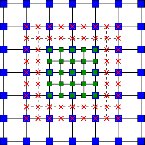
Figure 1: An illustration of 2 levels of grid refinement used in the code. The coarse grid points are shown as blue squares, the fine grid points as green ones and the ghost points (needed for the finite difference operators near the boundary of the fine grid) are marked as red crosses.

During the evolution, we update the values in the coarse grid points wherever possible with values from the fine (more accurate) grid (“restriction”). As coarse grid points that need restriction always coincide with a fine grid point, restriction simply consists of copying the value from the fine grid point to the coarse grid point.

We integrate our coupled system of hydrodynamics and BSSN equations via a 3rd order Total Variation Diminishing (TVD) Runge–Kutta integrator gottlieb98 . During each substep, the right-hand-sides (RHS) for the BSSN variables are calculated using finite differences (FD) where possible, that is, everywhere except at the ghost points (taking into account the size of the FD stencil) on all refinement levels. The state vector (consisting of all evolved variables on all possible grid points) is then evolved forward in time on all refinement levels where the RHS has been computed. After that, the state vector is updated in the ghost zones on each fine grid, via prolongation from the next-coarser grid, in a loop over refinement levels starting from the coarsest level. Finally, the solution on the coarser grids are updated via restriction from the finer grids in a second loop over refinement levels starting from the finest refinement level.

When interpolating metric information from the grid to the particles, we first find out which refinement level to interpolate from. Obviously, we want to use the finest possible refinement level in order to get the most accurate metric information on the particles. We therefore start on the finest refinement level and check whether the considered particle is located inside this grid. If it is, we perform the interpolation the same way as described in rosswog21a . If it is not, we move on to the next refinement level. We repeat until the interpolation can be performed or we reach the coarsest refinement level. Handling particles that leave the coarsest grid is not necessary for the cases presented here, but it will be implemented for future studies of merger ejecta.

2.1.3 Particle–mesh coupling: A MOOD approach

A crucial step in our approach is the mapping of $T_{\mu\nu}$, originally known at the particle positions, to the mesh (“P2M-step”) and the mapping of the metric acceleration terms $(dS_{i}/dt)_{\rm met}$ and $(de/dt)_{\rm met}$ from the mesh to the particle positions (“M2P-step”), see Eqs. (12) and (17). In this paper, we provide a further refinement of the P2M-step, see below, whereas the M2P-step is the same as in our original paper rosswog21a .

We map a quantity $A$ known at particle positions $\vec{r}_{p}=(x_{p},y_{p},z_{p})$ to the grid point $\vec{r}_{g}$ via

$$A_{g}=A(\vec{r}_{g})=\frac{\sum_{p}V_{p}A_{p}\,\Psi_{g}(\vec{r}_{p})}{\sum_{p}V_{p}\,\Psi_{g}(\vec{r}_{p})},$$ (20)

where $V_{p}=\nu_{p}/N_{p}$ is a measure of the particle volume. We construct the functions $\Psi$ as tensor products of 1D shape functions

$$\Psi_{g}(\vec{r}_{p})=\Phi\left(\frac{|x_{p}-x_{g}|}{l_{p}}\right)\Phi\left(\frac{|y_{p}-y_{g}|}{l_{p}}\right)\Phi\left(\frac{|z_{p}-z_{g}|}{l_{p}}\right),$$ (21)

where $l_{p}=V_{p}^{1/3}$. After extensive experimenting, we had settled in the original paper on a hierarchy of shape functions that have been developed in the context of vortex methods cottet00 .

The interpolation quality of the shape functions is closely related to the order with which they fulfill the so-called moment conditions cottet00

$$\sum_{q}x_{q}^{\alpha}\Phi(x_{q}-x)=x^{\alpha}\quad{\rm for}\quad 0\leq|\alpha|\leq m-1,$$ (22)

for points located at $x_{q}$. This means that the interpolation is exact for polynomials of a degree less than or equal to $m-1$ and such an interpolation is said to be “of order $m$” cottet00 . Good interpolation quality, however, does not automatically guarantee the smoothness of the shape functions, understood as the number of continuous derivatives. In fact, a number of shape functions that are commonly used, e.g. in particle-mesh methods for plasmas, are of low smoothness only and this can introduce a fair amount of noise in simulations. Being of higher order $m$, however, comes at the price of a larger stencil and therefore at some computational expense. Positive definite functions can only be maximally of order two monaghan92 , for higher orders the shape functions need to contain negative parts which can become problematic when the particle distribution within the kernel is far from being isotropic. A particularly disastrous case is encountering a sharp (e.g. stellar) surface. Here, violent Gibbs-phenomenon like oscillations can occur that can lead to unphysical results. For this reason we have implemented a hierarchy of kernels, so that the highest order shape functions can be used when it is safe, and less accurate, but more robust functions are used when it is not. How this is decided and implemented is described below.

Last, but not least, another characteristics of shape functions is their highest involved polynomial degree (“degree”). In this work we use smooth shape functions of high order that were constructed by Cottet et al. cottet14 . We follow their notation of using $\Lambda_{p,r}$ for a function that is of order $p+1$ (i.e., reproduces polynomials up to order $p$) and of smoothness $C^{r}$. Our chosen shape functions are the following:

1. the $\Lambda_{4,4}$-kernel (order 5, regularity $C^{4}$ and degree 9) cottet14

   $$\Lambda_{4,4}(|x|)=$$

   $$\left\{\begin{array}[]{lll}1-\dfrac{5}{4}|x|^{2}+\dfrac{1}{4}|x|^{4}-\dfrac{100}{3}|x|^{5}+\dfrac{455}{4}|x|^{6}&\\[8.53581pt] -\dfrac{295}{2}|x|^{7}+\dfrac{345}{4}|x|^{8}-\dfrac{115}{6}|x|^{9},&|x|<1,\\[11.38109pt] -199+\dfrac{5485}{4}|x|-\dfrac{32975}{8}|x|^{2}&\\[8.53581pt] +\dfrac{28425}{4}|x|^{3}-\dfrac{61953}{8}|x|^{4}+\dfrac{33175}{6}|x|^{5}&\\[8.53581pt] -\dfrac{20685}{8}|x|^{6}+\dfrac{3055}{4}|x|^{7}-\dfrac{1035}{8}|x|^{8}&\\[8.53581pt] +\dfrac{115}{12}|x|^{9},&1\leq|x|<2,\\[11.38109pt] 5913-\dfrac{89235}{4}|x|+\dfrac{297585}{8}|x|^{2}&\\[8.53581pt] -\dfrac{143895}{4}|x|^{3}+\dfrac{177871}{8}|x|^{4}-\dfrac{54641}{6}|x|^{5}&\\[8.53581pt] +\dfrac{19775}{8}|x|^{6}-\dfrac{1715}{4}|x|^{7}+\dfrac{345}{8}|x|^{8}&\\[8.53581pt] -\dfrac{23}{12}|x|^{9},&2\leq|x|<3,\\[11.38109pt] 0,&{\rm else}.\end{array}\right.$$ (34)

2. $\Lambda_{2,2}$ kernel (order 3, smoothness $C^{2}$, degree 5 cottet14

   $$\Lambda_{2,2}(|x|)=\left\{\begin{array}[]{llr}1-|x|^{2}-\dfrac{9}{2}|x|^{3}+\dfrac{15}{2}|x|^{4}&\\[8.53581pt] -3|x|^{5},&\;|x|<1,\\[11.38109pt] -4+18|x|-29|x|^{2}&\\[5.69054pt] +\dfrac{43}{2}|x|^{3}-\dfrac{15}{2}|x|^{4}+|x|^{5},&\;1\leq|x|<2,\\[11.38109pt] 0,&\;{\rm else}.\end{array}\right.$$ (40)

3. and, finally, the $M_{4}$ kernel (order 2, smoothness $C^{2}$, degree 3) cottet00

   $$M_{4}(x)=\left\{\begin{array}[]{llr}\dfrac{1}{6}\big{(}2-|x|\big{)}^{3}-\dfrac{2}{3}\big{(}1-|x|\big{)}^{3},&|x|<1,\\[11.38109pt] \dfrac{1}{6}\big{(}2-|x|\big{)}^{3},&1\leq|x|<2,\\[11.38109pt] 0,&{\rm else.}\end{array}\right.$$ (44)

Note that $\Lambda_{4,4}$ and $\Lambda_{2,2}$ are, differently from usual SPH-kernels, not positive definite. The supports of these kernels are sketched (for a 2D example) in Fig. 2. We apply a hierarchy of these kernels starting with $\Lambda_{4,4}$ followed by $\Lambda_{2,2}$ and we use the safest (positive definite, but least accurate) kernel $M_{4}$ as a “parachute.”

In the original paper we applied a heuristic method based on the particle content of the neighbour cells to decide which kernel to use. Instead of this, we use here a Multidimensional Optimal Order Detection (MOOD) method. The main idea is to use a “repeat-until-valid” approach, that is, to use the most accurate kernel that does not lead to any artifacts. To detect artifacts we check whether the resulting grid values of $T^{g}_{\mu\nu}$ are outside of the range of the values of the contributing particles, see below. This strategy is actually similar to MOOD approaches that are used in hydrodynamics; see, for example, diot13 . Specifically, we proceed according to the following steps:

1. Start with the highest order kernel $\Lambda_{4,4}$ for the mapping.

2. Check whether the $\Lambda_{4,4}$-result is acceptable: if all components of $T^{g}_{\mu\nu}$ at a given grid point are inside of the bracket $[T^{\rm min}_{\mu\nu},T^{\rm max}_{\mu\nu}]$, where the maximum and minimum values refer to the particles inside the $\Lambda_{4,4}$ support, we accept the $\Lambda_{4,4}$-mapping. Otherwise, we consider the mapping as questionable and proceed to the next kernel, $\Lambda_{2,2}$.

3. Check whether the $\Lambda_{2,2}$-result is acceptable: as in the previous step, we check whether the grid-result is outside of the bracket given by the particles in the support of $\Lambda_{2,2}$. If it is not, the $\Lambda_{2,2}$-mapping is accepted.

4. If also the $\Lambda_{2,2}$-result is not acceptable, we resort to our “parachute” solution, the positive definite $M_{4}$-mapping.

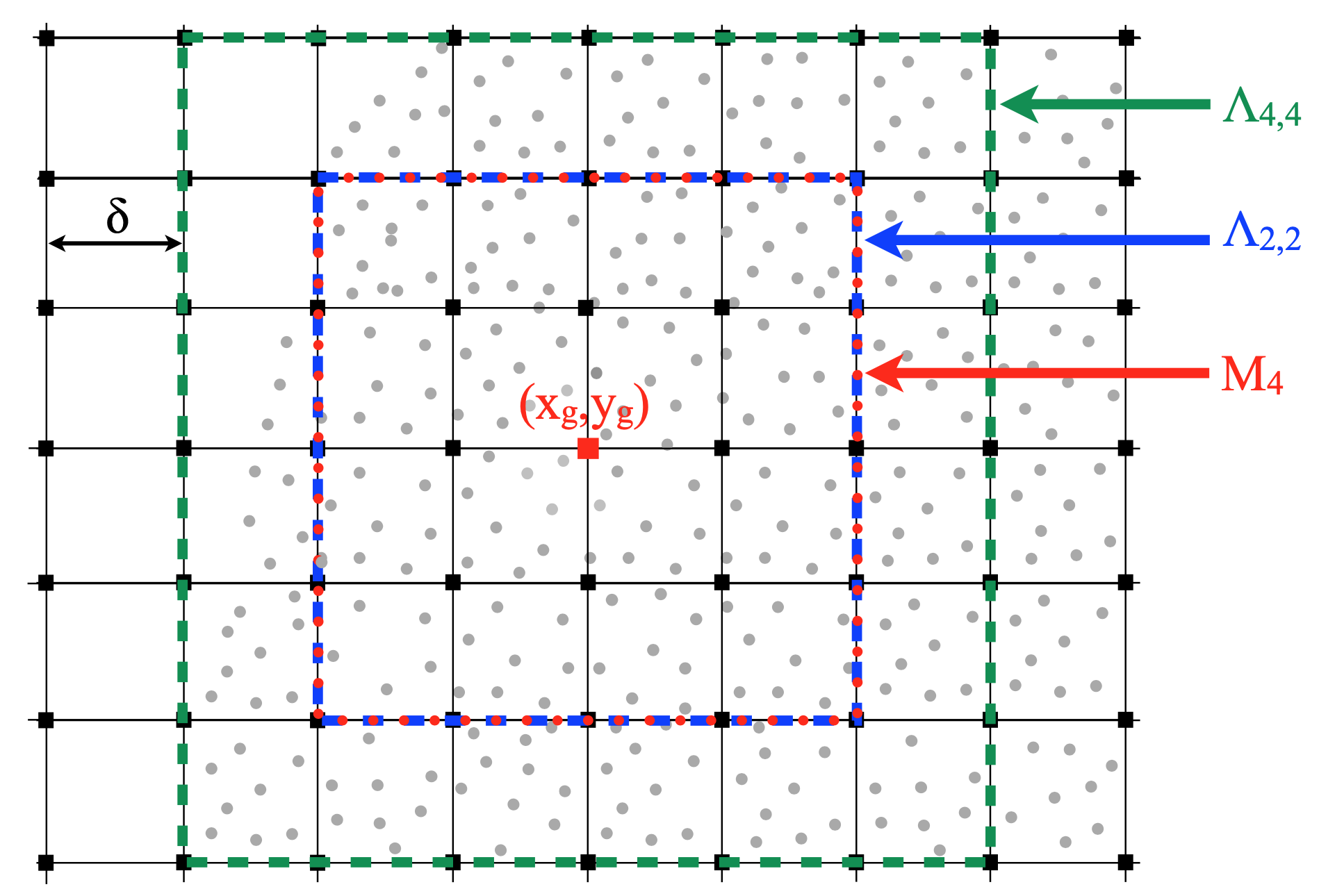
Figure 2: 2D sketch of the support sizes for the different kernels that are used in the MOOD-mapping for a specific grid point (red square). The green square indicates the support of the $\Lambda_{4,4}$-kernel, blue refers to $\Lambda_{2,2}$ and red to the “parachute” kernel $M_{4}$.

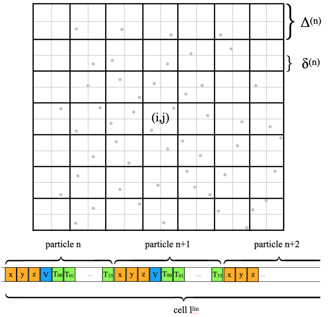
Figure 3: For an efficient mapping of the particle-$T_{\mu\nu}$ to the gravity grid on refinement level $n$ (on which the spacetime is evolved; grid spacing $\delta^{(n)}$; thin lines), we employ an additional hash grid with twice the grid-spacing ($\Delta^{(n)}$; thick lines). This is illustrated for the 2D-case in the upper part of the figure. The actual particle data needed for the mapping is stored in a cache-friendly linear array, see the lower part of the figure and the main text for more details.

Efficient implementation via a hash grid.

The tasks involved in the P2M-step are a) identify all particles that contribute to any given grid point, see Eq. (20), that is, those particles that are within the (tensor-product) support of the grid point’s kernel, b) loop over all grid points and add the particle $T_{\mu\nu}$-contributions.

We have implemented an efficient P2M-step that involves a hash grid at each refinement level $n$. The mesh size of our hash grid $\Delta^{(n)}$ is chosen to be twice the mesh size of the gravity grid, $\delta^{(n)}$, see upper part of Fig. 3 for an illustrating sketch in 2D. The reason why we chose a factor of two is that when updating the stress–energy tensor at a given gravity grid point, we need to collect the contributing particles from the hash grid. We do not want to have to check too many hash grid cells, so the hash grid cells should be larger than the gravity grid cells. On the other hand, they should not be too large, since then we would loop over many particles that in the end do not contribute to the grid point. A factor of two fulfils these criteria and makes the involved details (e.g., getting the hash grid indices from the gravity grid indices) very simple.

For performance reasons we store the data needed in the P2M-mapping process in a simple linear cache-array. The hash grid is only “virtual” in the sense that its structure is only needed to identify particles belonging to the same hash grid cell, but the data is actually stored in the linear cache-array. We first identify the 3D indices $(i,j,k)$ of the hash grid cell that contains the particle. These indices are then translated into a single index in our linear cache-array via $l^{\rm lin}=i+(j-1)n_{x}+(k-1)n_{x}n_{y}$, where $n_{x},n_{y},n_{z}$ are the numbers of hash grid cells in the $x$-, $y$- and $z$-direction on the current mesh refinement level. The index $l^{\rm lin}$ labels a segment in the cache-array that contains all the data associated with the particle in hash grid cell $(i,j,k)$ that is needed for the mapping. Since all data is stored in exactly the order in which it is needed, this approach guarantees virtually perfect cache efficiency.
The particles are filled into this hash grid as follows:

• In one first linear loop over the particles, each particle determines in which hash cell $(i,j,k)$ it is located. Each of the hash cells keeps track of how many particles it contains.

• After this loop, we can quickly count the number of entries, so that each ($i,j,k$) hash cell knows how many entries there are in the cache-array corresponding to the previous cells. In other words, after this (very fast) counting step, each hash grid cell knows the starting and finishing index that define the cache-array section storing all the properties of the particles contained in this ($i,j,k$) hash cell. Hence, all subsequent summations can be performed very efficiently.

• In another linear loop, those particle properties that are needed during the actual mapping are filled into the 1D array in exactly the same order in which they will be addressed during the mapping step (position, particle volume, stress–energy tensor components): $(x,y,z,V,T_{00},T_{0x},...,T_{zz})$. The resulting cache-array is sketched in the bottom part of Fig. 3. This cache-array approach has the advantage that the array has a fixed maximum length of 14 times the SPH particle number. We apply this mapping sequentially for each grid refinement level. If all particles are contained in the grid of a given level, the cache-array is completely filled, otherwise it is shorter since it does not contain entries from the particles outside the grid. Most importantly, the cache-array has to be allocated only once during the simulation, its size is known at compile time, and it can be used for every refinement level as a memory-efficient, “read-only” data structure in the P2M-step.

• The actual contribution-loop for each grid cell is then performed by checking the particle content of each potentially contributing hash cell and, if applicable, the particle contribution is added according to Eq. (20).

Compared to our initial, straightforward implementation, the above described cache-efficient P2M-step is more than 20 times faster for the simulations shown in this paper.

2.1.4 Code performance

Table 1: Breakdown of the time spent in different parts of the code. The different parts of the code are, in order: computation of the right-hand-sides (RHSs) in the hydro (SPH) and BSSN equations, mapping of the stress–energy tensor from the particles to the grid (P2M), mapping of the metric from the grid to the particles (M2P), restriction operators, prolongation operators, and finally the state vector update (see Sec. 2.1 for more details). Note that not all parts of the code are listed, so numbers do not add up to 100%. The symbols LR, MR and HR refer to low, medium and high resolution, see Sec. 3.1.

resolution	hydro RHS	BSSN RHS	P2M	M2P	restriction	prolongation	update state vector
LR	29.5%	33.6%	12.1%	1.8%	1.4%	5.8%	8.7%
MR	31.3%	31.9%	17.2%	1.7%	0.6%	3.5%	6.5%
HR	35.9%	23.1%	14.1%	1.7%	0.6%	3.6%	7.1%

The code is written in modern Fortran, except for the C++ routines which we extracted from McLachlan from the Einstein Toolkit in order to be able to evolve the spacetime. Currently the code is parallelized for shared memory architectures using OpenMP directives and pragmas. As the time spent in different parts of the code depends on the particle distribution, it is impossible to uniquely quantify the performance, but based on the simulations presented here, we can give some representative numbers.

In Table 1 we give a breakdown of how the time is spent in various important parts of the code for representative low, medium and high resolution runs. As can be seen, the major part of the time is spent in the hydrodynamics and spacetime evolution routines with additional significant time spent in the mapping of the stress–energy tensor to the grid. Running the code on compute nodes equipped with 128 AMD EPYC 7763 processors it initially takes 1.3, 3.2, 7.8 minutes to evolve one code unit of time at low, medium and high resolution respectively. This is maintained for the duration of the inspiral but as smaller time steps are required for hydrodynamic stability during and after the merger, the times required to evolve 1 code unit of time at the end are 2.2, 5.1 and 11.3 minutes at low, medium and high resolution, respectively. The memory usage for one of the medium resolution runs presented here is about 30 GB.
The OpenMP scaling is decent, but can certainly be improved. Scaling experiments show a speedup of about 43 on 128 cores.

2.2 Initial data

A crucial ingredient for every relativistic simulation are initial data (ID) that both satisfy the constraint equations and accurately describe the physical system of interest. In the following, we describe how we compute such ID for BNS, that we subsequently evolve with SPHINCS_BSSN.

2.2.1 Quasi-equilibrium BNS with LORENE

The library LORENE computes ID for relativistic BNS under the assumption of “quasi-equilibrium,” see Gourgoulhon:2000nn and (gourgoulhon20123+1, , Sec. 9.4) for more details. This assumption states that the radial velocity component of the stars is negligibly small compared to the azimuthal one and the orbital evolution is essentially realized via a sequence of circular orbits. Equivalently, one assumes that a helical Killing vector field exists. This assumption is reasonably well justified since at a separation of $\sim 50$ km, the time derivative of the orbital period (at the second post-Newtonian level) is about $2\%$ of the period itself Gourgoulhon:2000nn .

LORENE allows to compute ID for corotational and irrotational binaries. Since any neutron star viscosity is too small to spin up the neutron stars during the rapid final inspiral stages to corotation bildsten92 ; kochanek92 ; Gourgoulhon:2000nn , the irrotational case is generally considered more realistic, but mergers with rapidly spinning neutron stars can lead to interesting effects and the corresponding simulations are now feasible bernuzzi14 ; dietrich15 ; dudi21 . In this paper, we restrict ourselves to irrotational binaries. Another assumption that is made in LORENE is the conformal flatness of the spatial metric $\gamma_{ij}$. This is a commonly made approximation which substantially simplifies the solving of the constraint equations.

LORENE provides spectral solutions that can be evaluated at any point. By default, the code BinNS in
LORENE allows to export the LORENE ID to a Cartesian grid. However, this is not sufficient for our purposes, since we need to evaluate the solution not only on our refined mesh, but also at the positions of the SPH particles. Hence, we have extended BinNS to evaluate the spectral data at any given spacetime point. We have further linked the relevant functions in BinNS to our own code that sets up the ID for SPHINCS_BSSN and is called SPHINCS_ID. Since in the original version of LORENE, BinNS was able to handle only BNS with single polytropic EOS, we extended it to read and export also configurations with piecewise polytropic and tabulated EOS such as those available in the CompOSE database compose . In other words, all the needed information that LORENE provides about the BNS is accessible within SPHINCS_ID. Despite having these capabilities, we restrict ourselves to purely polytropic equations of state in this first study.

2.2.2 The “Artificial Pressure Method” for binary systems

SPH initial conditions are a delicate subject. The particle distribution has to, of course, accurately represent the physical system under consideration (e.g., densities and velocities), but there are additional requirements concerning how the particles are actually distributed, see, for example, rosswog15b ; diehl_rockefeller_fryer_riethmiller_statler_2015 ; arth_2019 . The particle arrangement should be stable, so that in an equilibrium situation, the particles ideally should not move at all. Many straightforward particle arrangements (such as cubic lattices), however, are not stable and particles quickly start to move if set up in this way. The reason is a “self-regularization” mechanism built into SPH that tries to locally optimize the particle distribution (see, e.g., Sec. 3.2.3 in rosswog15c for more details). To make things even harder, the particles should be distributed very regularly, but not in configurations with pronounced symmetries, since the latter can lead to artifacts, for example if a shock propagates along such a symmetry direction. Last, but not least, the SPH particles should ideally have practically the same masses/baryon numbers, since for large differences numerical noise (i.e., small scale fluctuations in the particle velocities) occurs that can have a negative impact on the interpolation accuracy.

All of these issues are addressed by the “Artificial Pressure Method” (APM) to optimally place SPH particles. The method has been suggested in a Newtonian context rosswog20a and was recently generalized to the case of general relativistic neutron stars rosswog21a . In this work, we go one step further and apply the APM in the construction of relativistic binary systems.

The main idea of the APM is to start from a distribution of equal-mass particles and let the particles find the positions in which they minimize their density error with respect to a desired density profile. In other words, each particle has to measure in which direction the density error is decreasing and move accordingly.

In practice, this is achieved by assigning to each particle $a$ an “artificial pressure,” $\pi_{a}$, that is based on the discrepancy between actual, measured SPH-density, $\rho_{a}$, and the desired profile value at the position of the particle, $\rho^{P}(\vec{r}_{a})$:

$$\pi_{a}={\rm max}\left(1+\frac{\rho_{a}-\rho^{P}(\vec{r}_{a})}{\rho^{P}(\vec{r}_{a})},0.1\right)$$ (45)

where the max-function has been used to avoid negative pressures. For more details of the method we refer to the original paper rosswog20a . This pressure is then used in a position update formula that is modelled after a fluid momentum equation (see rosswog20a for the derivation):

$${\delta\vec{r}_{a}}^{\rm APM}=-\frac{1}{2}h_{a}^{2}\nu_{0}\sum_{b}\frac{\pi_{a}+\pi_{b}}{N_{b}}\nabla_{a}W_{ab}(h_{a}),$$ (46)

where the quantities have the same meaning as in the fluid section, Sec. 2.1.1, and $\nu_{0}$ is the baryon number desired for each particle (equal to the total baryon mass divided by the chosen particle number). Iterations with such position updates drive the particles towards positions where they minimize their density error. It does, however, not necessarily guarantee that the particle distribution is locally regular and provides a good interpolation accuracy (for corresponding criteria see, e.g., Sec. 2.1 in rosswog15c ). To achieve this, we add a small additional “regularization term” gaburov11

$${\delta\vec{r}_{a}}^{\rm reg}=h_{a}^{4}\sum_{b}W_{ab}(h_{a})\hat{e}_{ab},$$ (47)

where $\hat{e}_{ab}=(\vec{r}_{a}-\vec{r}_{b})/|\vec{r}_{a}-\vec{r}_{b}|$, so that the final position update reads

$$\vec{r}_{a}\rightarrow\vec{r}_{a}+(1-\zeta){\delta\vec{r}_{a}}^{\rm APM}+\zeta{\delta\vec{r}_{a}}^{\rm reg}.$$ (48)

The parameter $\zeta$ determines how important the local regularity requirement on the particle distribution is compared to the accuracy with which the desired density profile is reproduced. Since our main emphasis is on reproducing the desired density, the value of $1-\zeta$ should not be too much below unity, but the exact parameter value is only of minor importance. We find good results for $\zeta=0.05$, which we use throughout this paper. We start the APM iteration with an initial particle distribution obtained by first placing particles on spherical surfaces, as described in B.1, and then slightly moving them away from the surfaces by a small random displacement. We noticed that the use of such random displacements led to better results of the APM procedure.

A crucial ingredient of the method is the placement of the “boundary” or “ghost” particles. These serve as a shield around the star to prevent the real particles from exiting the surface of the star during the APM iteration. The artificial pressure that we assign to these ghost particles is a few times higher (we use three times) than the maximum value inside the star. This is to ensure that particles that approach the stellar surface from the inside, see an increasing pressure gradient which keeps them inside the stellar surface. Since the stars in a close binary system are tidally deformed, the ghost particles have to be placed in a way that allows the real particles to model the surface geometry, see B.2 for more details on how this is achieved. Once the APM iteration has converged, the ghost particles are discarded. Figure 4 shows the ghost particles (red) placed around the real particles (black) on spherical surfaces before and after applying the APM, for one star of one of our simulations (run LR_2x1.3_G2.00, see Table 2).

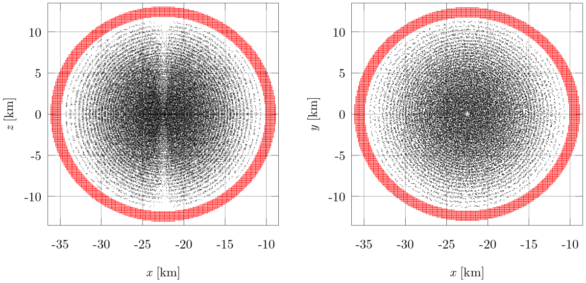
(a) Initial particle distribution used for the APM iteration. The particles are placed on spherical surfaces first (see B.1 for more details), and then randomized by a small amount.

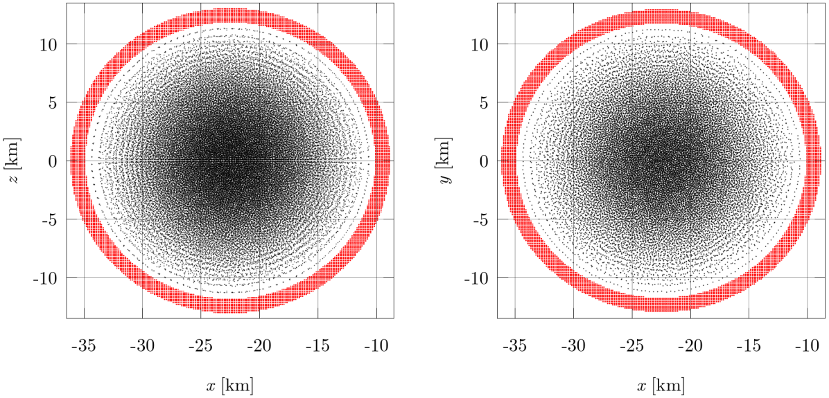
(b) At the end of the APM iteration, the particles form a very regular, “glass-like” structure.

Figure 4: Shown are the particle distributions before (a) and after (b) the APM iteration for one neutron star of our run LR_2x1.3_G2.00, see Table 2. The physical SPH particles are shown in black and the ghost/boundary particles (discarded after the APM iteration) are shown in red. The plots are cuts through the $xz$ and $xy$ plane, within $y\in[-1.18,1.18]$km and $z\in[-1.18,1.18]$km.

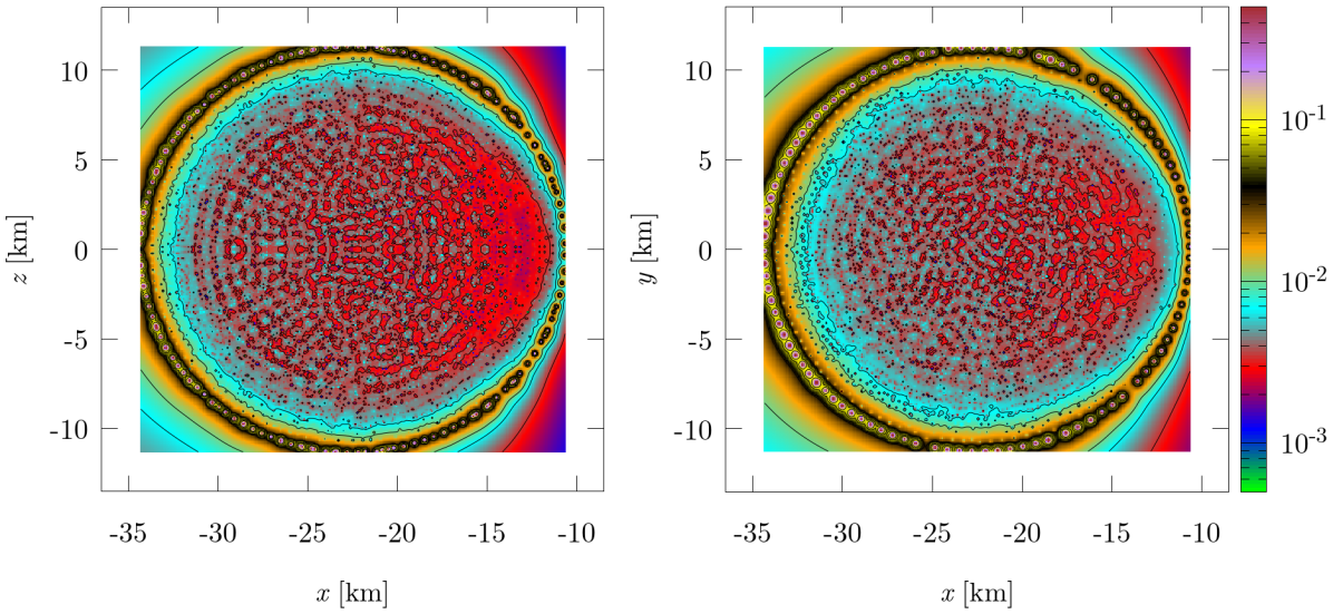
Figure 5: Typical relative density errors (i.e., relative difference between the SPH kernel density estimate at particle positions and the LORENE density) after the APM iteration on the $xz$ and $xy$ planes (the contours are computed using particles in $y\in[-0.44,0.44]$km and $z\in[-0.44,0.44]$km, respectively). The same star as in Figure 4 (LR_2x1.3_G2.00, see Table 2) is shown. Typical density errors in the bulk of the star are below 1%, whereas in the hard-to-resolve surface layers, errors can reach 10%.

After each step of the APM iteration, the particle positions are reset so that the center of mass of the particle distribution coincides (within machine precision) with the stellar center of mass given by LORENE. In addition, at each step of the APM iteration, the particle positions are reflected about the $xy$ plane, to impose exact equatorial-plane symmetry.

Once the APM iteration with particles of equal baryon number, $\nu_{0}$, has converged, we perform one single, final correction of the individual particle baryon numbers, $\nu_{a}$. To this end we first calculate the SPH particle number density,

$$\tilde{N}_{a}=\sum_{b}W_{ab}(h_{a}),$$ (49)

and then assign to each particle the “desired” baryon number

$$\nu_{a}^{\rm des}=\frac{N_{a}}{\tilde{N}_{a}},$$ (50)

where $N_{a}$ is the density according to LORENE. The baryon number assigned to each particle is a “capped” version of $\nu_{a}^{\rm des}$ in (50), so that $\nu_{a}$ remains in the interval $[\sqrt{2}\nu_{o},\nu_{o}/\sqrt{2}]$ and the baryon number ratio is $\leq 2$. This correction step changes the baryon masses only moderately, but improves the density estimate in the outer layers by roughly an order of magnitude.

This method allows to obtain a low baryon number ratio on each star, separately. In order to have a low baryon number ratio overall, that is, across both stars, we set the particle numbers within each star to have a similar ratio as the binary mass ratio. For more details, see B.1.

Figure 5 shows contour plots of the relative difference between the LORENE mass density and the SPH kernel estimate of the mass density performed on the final particle distribution (including the one update on the baryon number). In the bulk of the stars the errors are lower than $\sim 1$%. Only in the surface layers are the errors larger. Here, the very steep physical density gradients are difficult to capture at finite resolution with nearly equal SPH particle masses. These layers will adjust slightly at the beginning of a simulation, trying to find a true numerical equilibrium.

As the last comment, we note that, for equal-mass BNS, we use the APM to place particles within one star only. The particles in the second star are obtained by simply reflecting those on the first star with respect to the $yz$ plane. In this way, the symmetry of the system is preserved also at the level of the particle distribution.

2.2.3 Initial values for the SPH particles

Once the final particle locations have been found, we need to assign particle properties according to the
LORENE solution. The computing frame fluid velocity in Eq. (3) is related to the fluid velocity with respect to the Eulerian observer $v^{i}_{\mathrm{Eul}}$ (provided by LORENE) by

$$v^{0}=1,\quad v^{i}=\alpha\,v^{i}_{\mathrm{Eul}}-\beta^{i}.$$ (51)

The generalized Lorentz factor $\Theta$ can then be computed from $v^{i}$ using Eq. (2). The baryon number per particle $\nu$ is determined as described in B.1 and Sec. 2.2.2. The smoothing length $h$ of each particle is computed so that each particle has exactly 300 contributing neighbours in the density estimate, as in SPHINCS_BSSN. Then, knowing $\nu$ and $h$, the density variable $N$ can be computed using Eq. (8), and the local rest frame baryon number density $n$ is computed inverting Eq. (7),

$$n=\dfrac{N}{\sqrt{-g}\;\Theta}.$$ (52)

The local rest frame baryon mass density is then

$$\rho_{\rm rest}=n\,m_{0},$$ (53)

where $m_{0}$ is the average baryon mass. The specific internal energy $u$ and the pressure $P$ are then computed using the EOS, starting from $\rho_{\rm rest}$.

2.2.4 BSSN initial data on the refined mesh

The ID for the BSSN variables is computed straightforwardly by first importing the LORENE ID for the standard 3+1, or ADM, variables to each level of the mesh refinement hierarchy, and then computing the BSSN variables from them using a routine extracted from the McLachlan thorn from the Einstein Toolkit loeffler12 . For the sake of clarity, we note that, for the runs shown in this paper, we use the initial values for the lapse function and the shift vector that LORENE provides.

3 Simulations

Table 2: Parameters of the performed simulations. The masses are gravitational masses in solar units. $\Gamma$ is the polytropic exponent and $K$ the corresponding constant in code units. The initial orbital angular velocity $\Omega_{0}$ is in units of rad/s. The quantity $h_{\rm min}$ is the minimal smoothing length during the evolution, $\Delta_{g}^{\rm min}$ is the grid resolution at the finest refinement level, and they are both given in m. $n_{\rm grid}$ is the number of grid points on each refinement level. All simulations start from a coordinate separation of $a_{0}=30.4748$ (corresponding to 45 km) and use 7 levels of grid refinement, with the outermost refinement level’s boundary at $\approx 2268$ km.

Masses [$M_{\odot}$]	$\Gamma$	$K$	$\Omega_{0}$ [rad/s]	# particles	$h_{\rm min}$ [m]	$n_{\rm grid}$	$\Delta_{g}^{\rm min}$ [m]	Name
2 $\times$ 1.3	2.00	100	1774	$5\times 10^{5}$	40	$121^{3}$	590	LR_2x1.3_G2.00
2 $\times$ 1.3	2.00	100	1774	$1\times 10^{6}$	183	$143^{3}$	500	MR_2x1.3_G2.00
2 $\times$ 1.3	2.00	100	1774	$2\times 10^{6}$	165	$193^{3}$	370	HR_2x1.3_G2.00
2 $\times$ 1.3	2.75	$3\times 10^{4}$	1772	$5\times 10^{5}$	338	$121^{3}$	590	LR_2x1.3_G2.75
2 $\times$ 1.3	2.75	$3\times 10^{4}$	1772	$1\times 10^{6}$	274	$143^{3}$	500	MR_2x1.3_G2.75
2 $\times$ 1.3	2.75	$3\times 10^{4}$	1772	$2\times 10^{6}$	224	$193^{3}$	370	HR_2x1.3_G2.75
2 $\times$ 1.4	2.00	100	1827	$5\times 10^{5}$	53	$121^{3}$	590	LR_2x1.4_G2.00
2 $\times$ 1.4	2.00	100	1827	$1\times 10^{6}$	70	$143^{3}$	500	MR_2x1.4_G2.00
2 $\times$ 1.4	2.00	100	1827	$2\times 10^{6}$	25	$193^{3}$	370	HR_2x1.4_G2.00
2 $\times$ 1.4	2.75	$3\times 10^{4}$	1823	$5\times 10^{5}$	307	$121^{3}$	590	LR_2x1.4_G2.75
2 $\times$ 1.4	2.75	$3\times 10^{4}$	1823	$1\times 10^{6}$	245	$143^{3}$	500	MR_2x1.4_G2.75
2 $\times$ 1.4	2.75	$3\times 10^{4}$	1823	$2\times 10^{6}$	192	$193^{3}$	370	HR_2x1.4_G2.75

In our original paper, we had focused on test cases where the outcomes are accurately known. These included shock tubes (exact result known), oscillating neutron stars in Cowling approximation and in dynamically evolved space times (in both cases oscillation frequencies are accurately known) and, finally, the evolution of an unstable neutron star that, depending on small initial perturbations, either transitions into a stable configuration or collapses and forms a black hole (results known from independent numerical approaches, e.g., font02 ; cordero09 ; bernuzzi10 ). In all of these benchmarks our results were in excellent agreement with established results.

Here, we want to take the next step towards more astrophysically motivated questions. In particular, we want to address for the first time the merger of two neutron stars with SPHINCS_BSSN.

3.1 Initial Setup

In this first study, we simulate two binary systems with $2\times 1.3$ M_⊙ and $2\times 1.4$ M_⊙, each time with a soft ($\Gamma=2.00$, $K=100$ in code units; $M_{\rm max}^{\rm TOV}\approx 1.64$ M_⊙) and a stiff ($\Gamma=2.75$, $K=30~{}000$ in code units; $M_{\rm max}^{\rm TOV}\approx 2.43$ M_⊙) EOS. Both equations of state are admittedly highly idealized, and in one of our next steps we will include the physical EOSs that are provided by the CompOSE database compose . Each of the simulations are run at three different resolutions: a) low-resolution (LR) with $5\times 10^{5}$ SPH particles and $121^{3}$ grid points on every refinement level, b) medium-resolution (MR) with $10^{6}$ SPH particles and $143^{3}$ grid points on each refinement level and c) high-resolution (HR) with $2\times 10^{6}$ SPH particles and $193^{3}$ grid points on each refinement level. All simulations start from a coordinate separation of 45 km, and employ seven refinement levels out to 1536 code units ($\approx$ 2268 km) in each direction. The parameters of the performed simulations are summarized in Table 2, the quoted numbers are accurate to $\sim$ 1%. Note that we also show the minimum smoothing length, $h_{\rm min}$, during a simulation. This is, of course, a quantity that adapts automatically according to the dynamics and that is not determined beforehand. For example, the $h_{\rm min}=40$ m in run LR_2x1.3_G2.00 is so small because the central object at very late times ($\sim$ 18 ms) collapses to a black hole. This is a very low resolution result, it should be interpreted with caution.

3.2 Results

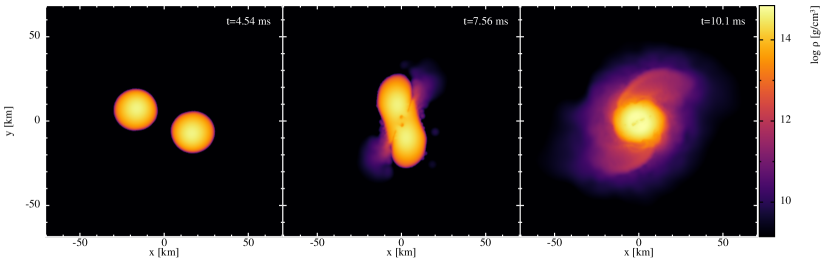
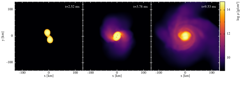
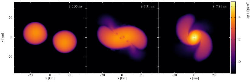
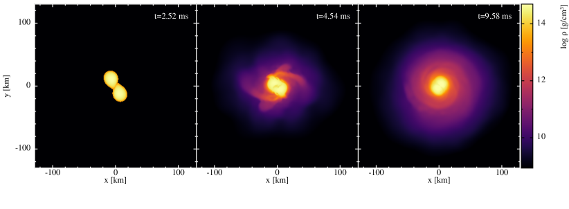
Figure 6: Density evolution of the simulations (top to bottom) HR_2x1.3_G2.00, HR_2x1.3_G2.75, HR_2x1.4_G2.00 and HR_2x1.4_G2.75, see Table 2 for the corresponding parameters.

In Fig. 6 we show snapshots of the rest-mass density evolution of the HR runs of our different binaries, with $t=0$ corresponding to the simulation start. Fig. 7 shows the evolution of the maximum density (left) and minimum lapse value (right) of the corresponding runs and Fig. 8 shows the quadrupole GW amplitudes $h_{\rm max}$ (for an observer located along the rotation axis; see A) times the distance to the observer $D_{\rm obs}$. These quadrupole approximation results are written out “on the fly” and they can be compared to the more accurate results that can be extracted in a post-processing step from the spacetime evolution, see below.

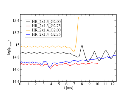
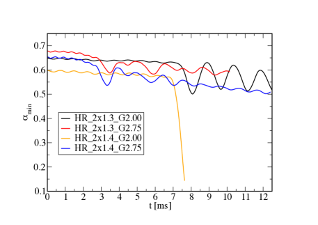
Figure 7: Evolution of the maximum density and the minimum lapse value for the HR-runs.

As expected, the cases with the soft EOS, where the stars are more compact and therefore closer to the point mass limit, show a substantially longer inspiral and chirp signal (lines 1 and 3 vs lines 2 and 4 in Fig. 8). Being more compressible, their peak density evolution is also more impacted by the merger, see the left panel of Fig. 7, and this is also reflected in the evolution of the minimum lapse value (right panel). In the cases with the stiff EOS, in contrast, where the stars are larger and more mass is at larger radii from the stellar centre, tidal effects are much more pronounced and effectively represent a short-range, attractive interaction damour09b ; radice20 . Therefore our binaries with stiff EOS merge within less than two orbital revolutions from the chosen initial separation. Being rather incompressible, the post-merger central densities are actually only moderately above the central densities of the initial individual stars, see Fig. 7, left panel, and also the lapse oscillations (right panel) are small. All of the remnants seem to evolve to more compact configurations, but of the shown cases only HR_2x1.3_G2.00 collapses to a black hole during the simulated times.

For the simulations afforded in this study, numerical resolution still has a noticeable effect on the inspiral as, for example, demonstrated by simulation HR_2x1.3_G2.00, which takes about one orbit more until merger than LR_2x1.3_G2.00 (upper right vs upper left in Fig. 8). The HR runs with the soft equation of state do show some signs of amplitude variations that could be attributed to eccentricity, whereas the low and medium resolutions do not seem to show that. We certainly do expect some eccentricity due to the assumptions going into the ID construction. As to why it is more pronounced in the HR case, it is possible that the low and medium resolution runs are short enough so that signs of eccentricity are washed out. Finally, these extracted waveforms are calculated from gauge dependent quantities and the amplitude variations could be entirely spurious. All investigated systems, apart from the $2\times 1.4$ M_⊙ cases with $\Gamma=2.00$, leave a stable remnant (at least on the simulation time scale) and therefore keep emitting gravitational waves. The exceptional case, see row three in Fig. 6, undergoes a prompt collapse to a black hole within $\sim$ 1 ms after merger (Fig. 7) which efficiently shuts off the gravitational wave emission (row three in Fig. 8). A collapse to a black hole is expected when the binary mass exceeds $\sim 1.5\times M_{\rm max}^{\rm TOV}$ hotokezaka11 ; bauswein13b ; koeppel19 ; kashyap21 , so the collapse in HR_2x1.4_G2.00 is actually expected given that $M_{\rm max}^{\rm TOV}$ is only 1.64 M_⊙ and the initial ADM mass of the system is 2.9M_⊙.

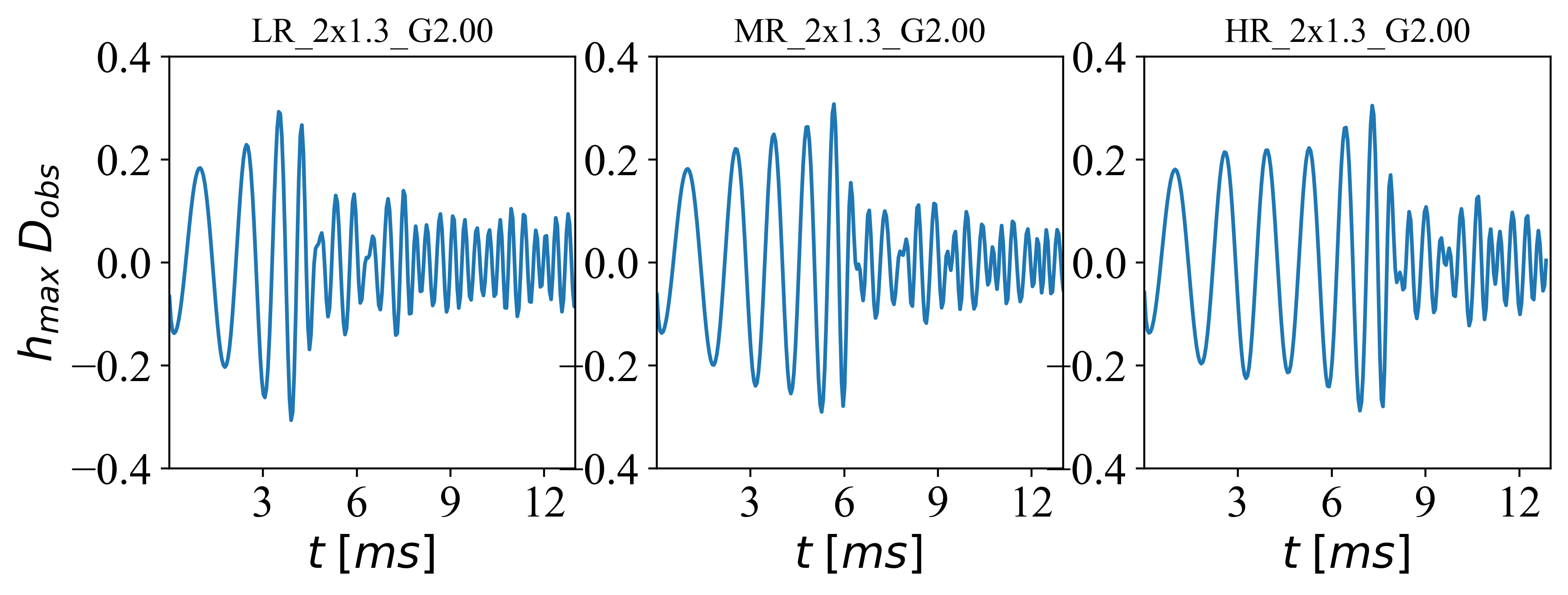
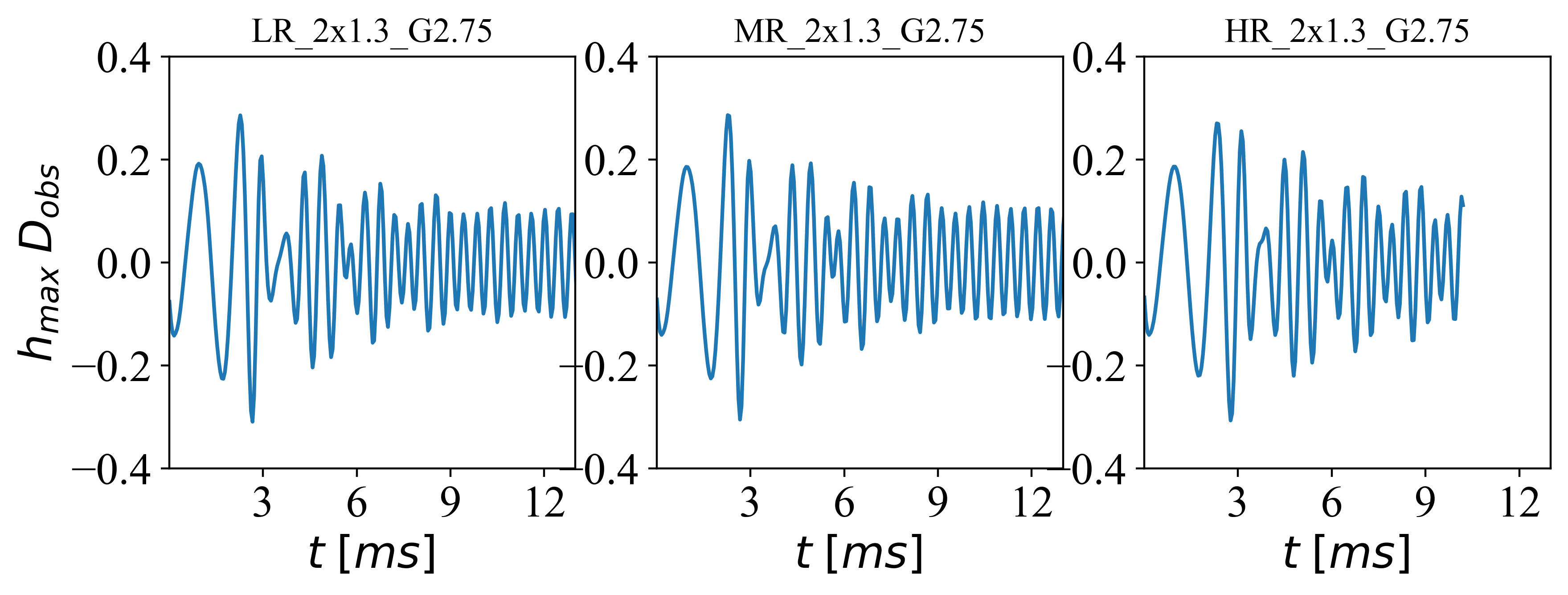
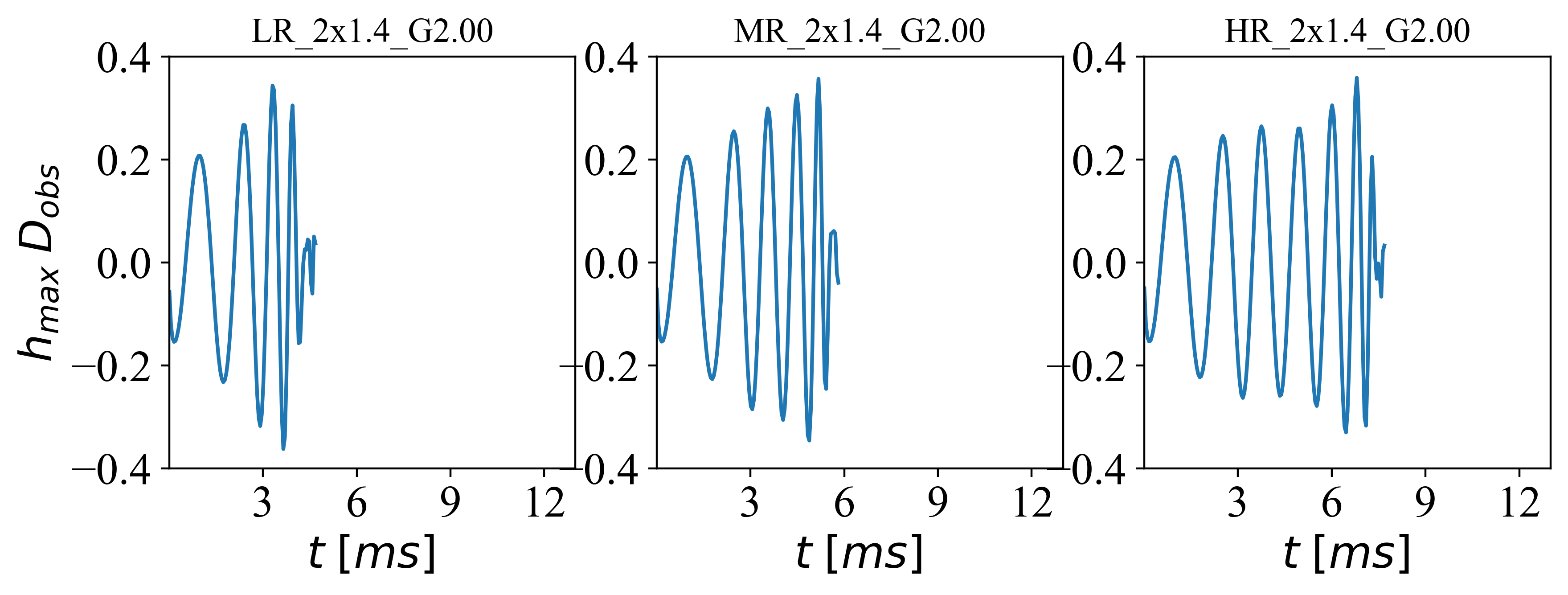
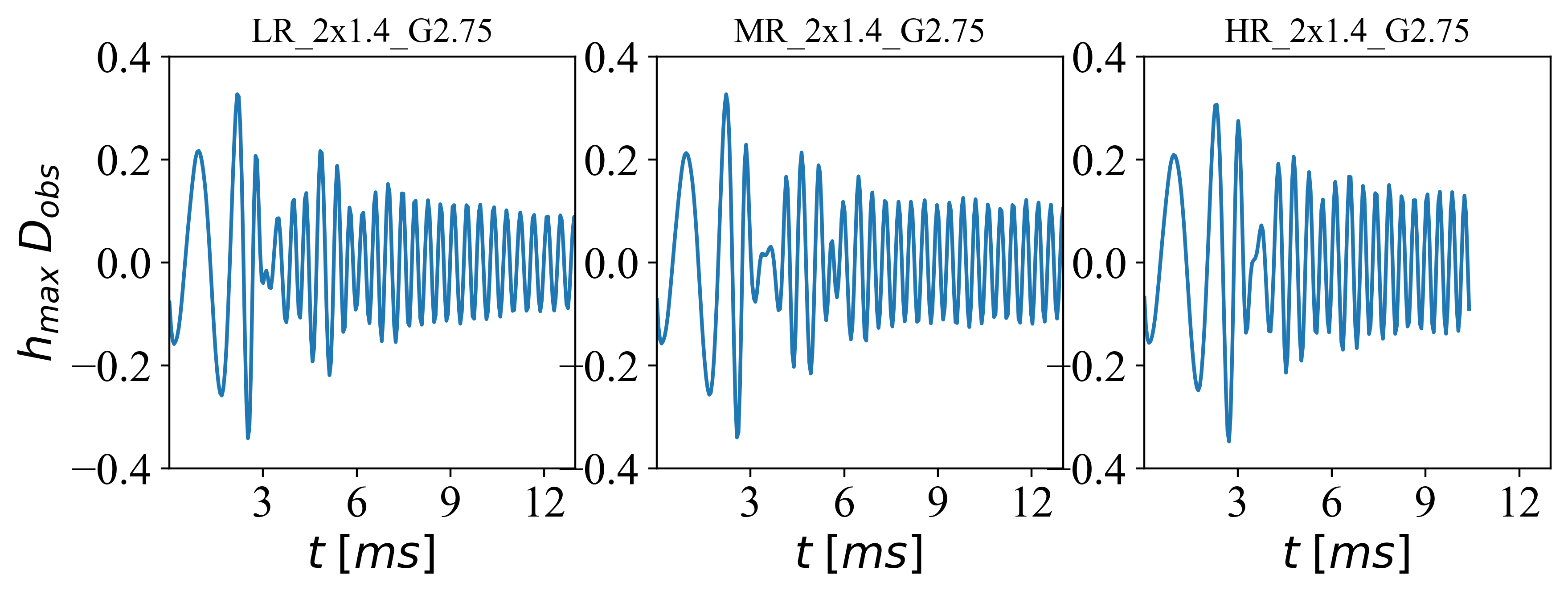
Figure 8: Gravitational wave amplitudes computed with the quadrupole formula, see A, for the simulations (top to bottom) HR_2x1.3_G2.00, HR_2x1.3_G2.75, HR_2x1.4_G2.00 and HR_2x1.4_G2.75, see Table 2. The quantity $D_{\rm obs}$ is the distance to the observer in code units, and $h_{\rm max}$ is the maximal amplitude for an observer located on the $z$ axis.

We have, in addition to using the quadrupole formula, also extracted gravitational waves based on the spacetime data using both thorn Extract and (in combination) thorns WeylScal 4 and Multipole from the Einstein Toolkit loeffler12 . The procedure was to read in metric data from our third coarsest refinement level at the times we had checkpoint data, run the wave extraction tools and finally use the formulae in A.2 to calculate the strain as well as the radiated energy and angular momentum. We used detectors at spheres of coordinate radii 50, 100, 150, 200, 250 and 300. We see very good agreement between the results from Extract and WeylScal 4, but as the WeylScal 4 waveforms are less noisy we only report on those results in the following.
In Fig. 9 we plot the radiated energy, $\Delta E$, and $z$-component of the angular momentum, $\Delta J_{z}$, as function of time for the system with two 1.4 M_⊙ neutron stars and $\Gamma=2.75$. The quantities are plotted as percentages of the initial ADM values of the spacetime, $E^{0}$ and ${J_{z}}^{0}$. We can clearly not yet claim convergence of these results as the rate of energy and angular momentum emission after merger increases significantly from the medium to high resolution runs and the behavior of the low resolution run is substantially different showing a decreasing rate of emission at late times.

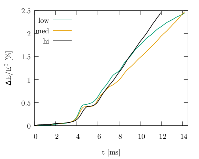
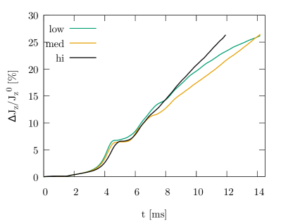
Figure 9: The accumulated radiated energy, $\Delta E$ (left plot), and $z$-component of the angular momentum, $\Delta J_{z}$ (right plot) in percent of the initial values, $E^{0}$ and ${J_{z}}^{0}$ for the system with two 1.4 M_⊙ neutron stars and $\Gamma=2.75$ extracted at the detector at coordinate radius R=300. In both plots the green, orange, black curves are for the low, medium and high resolution runs, respectively.

In Table 3, we list the final radiated energy at the end of our simulations, $\Delta E$, and$z$-component of the angular momentum, $\Delta J_{z}$, again as percentages of the initial ADM energy $E^{0}$ and angular momentum $\Delta J_{z}^{0}$ of the spacetime for a sample of our simulations. Note that in the simulations listed, the merger remnant has not yet collapsed to a black hole, hence the systems are still emitting strong gravitational waves. In addition, as we cannot claim that the quantities are converged, we can are unable to perform a conclusive comparison with, for example, the results of zappa18 , but for now we can only state that our simulations appear to be consistent.

Table 3: Percentage of radiated energy, $\Delta E$, and $z$-component of angular momentum, $\Delta J_{z}$, with respect to the initial ADM energy, $E^{0}$, and ADM angular momentum, $J_{z}^{0}$ for a sample of our simulations. As all simulations were not run for the same amount of time, we also list the simulation duration, $t_{\mathrm{end}}$.

Name	$t_{\mathrm{end}}$ [ms]	$\Delta E/E^{0}$ [%]	$\Delta J_{z}/\Delta J_{z}^{0}$ [%]
LR_2x1.3_G2.00	14.78	1.7	19.6
MR_2x1.3_G2.00	14.78	1.3	17.4
LR_2x1.3_G2.75	14.78	1.7	20.8
MR_2x1.3_G2.75	14.78	1.7	20.9
LR_2x1.4_G2.75	14.78	2.5	26.9
MR_2x1.4_G2.75	14.78	2.6	28.0
HR_2x1.4_G2.75	12.46	2.6	29.5

In Fig. 10 we show a comparison of the maximal strain amplitude extracted using either the quadrupole formula or the Weyl scalar $\Psi_{4}$. Here the strain from $\Psi_{4}$ is the sum of spin weight $-2$ spherical harmonic modes from $\ell=2$ to 4 evaluated on the $z$-axis ($\theta=0$ and $\phi=\pi/2$ to match the observer orientation) and then shifted in time (by about 1.54 ms) to account for the signal travel time to the detector. As can be seen, the quadrupole formula consistently underestimates the amplitude (especially after the merger; less so during the inspiral). This is in agreement with baiotti09 where it was found that the amplitudes could be over- or underestimated by more than 50% depending on the definition of density used. On the other hand, also in agreement with baiotti09 , the frequencies are well captured by the quadrupole formula.

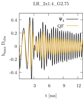
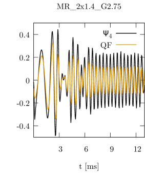
Figure 10: Comparison of the maximal strain amplitude as calculated by the extraction of $\Psi_{4}$ (black) and the quadrupole formula (QF, orange) for the simulations with two 1.4M_⊙ neutron stars and $\Gamma=2.75$. The strain from $\Psi_{4}$ is the sum of spin-weight -2 modes from $\ell=2$ to 4 evaluated on the z-axis ($\theta=0$) and shifted in time by 1.54 ms in order to align it with the quadrupole waveform. The quantity $D_{\rm obs}$ is the distance to the observer (code units), and $h_{\rm max}$ is the maximum amplitude for an observer located on the $z$ axis.

We also want to briefly illustrate a major advantage of our methodology: the treatment of the neutron star surface. Contrary to traditional Eulerian approaches, the sharp transition between the high-density neutron star and the surrounding vacuum does not pose any challenge for our method and no special treatment such as an “artificial atmosphere” representing vacuum is needed. The particles merely adjust their positions according to the balance of gravity and pressure gradients to find their true numerical equilibrium and vacuum simply corresponds to the absence of particles. Throughout the inspiral, the neutron star surface remains smooth and well-behaved without any “outliers,” see Fig. 11. This illustrates the quality of both the evolution code and the initial particle setup, see Sec. 2.2.2.

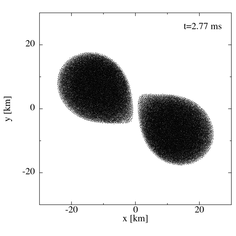
Figure 11: Particle positions (within $|z|<$ 1 km) in run HR_2x1.4_G2.75, see Table 2, prior to merger. Modelling the transition between the neutron star matter and vacuum represents a serious numerical challenge for Eulerian hydrodynamic approaches. In our approach, however, the stellar surface does not require any special treatment and it remains smooth and well-behaved during the inspiral without any “outlier particles.”

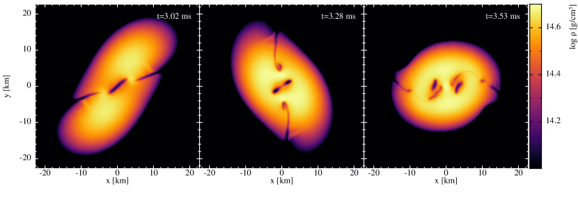
Figure 12: Evolution of the Kelvin–Helmholtz vortices in simulation HR_2x1.4_G2.75, see Table 2.

At the interface where the two neutron stars come into contact, a Kelvin–Helmholtz unstable shear layer forms. Although we are presently not modelling magnetic fields, it is worth pointing out that this shear layer is important for magnetic field amplification. In the resulting Kelvin–Helmholtz vortices initially present magnetic fields can be efficiently amplified beyond magnetar field strength price06 ; kiuchi14 ; kiuchi15 ; kiuchi18 , which obviously has a large astrophysical relevance for potentially increasing the maximum remnant mass, magnetically ejecting matter and for launching GRBs. Traditional SPH-approaches have been found to be challenged in resolving weakly triggered Kelvin–Helmholtz instabilities agertz07 ; mcnally12 , but these problems are absent in the modern high-accuracy SPH-approach that is implemented in SPHINCS_BSSN, mostly due to the reconstruction procedure in the dissipative terms and to the much more accurate gradients than those used in “old school SPH.” To illustrate the Kelvin–Helmholtz instabilities that emerge in our SPHINCS_BSSN simulations, we show the density near the shear interface between the two stars for our simulation HR_2x1.4_G2.75 in Fig. 12. In this simulation four vortices are initially triggered, that subsequently move inwards and finally merge. While the initial stages show an almost perfect symmetry, see Fig. 12, tiny asymmetries, seeded by the numerics, are amplified by the Kelvin–Helmholtz instability and finally lead to a breaking of exact symmetry. It goes without saying that such a breaking of perfect symmetry will also occur in nature.

The Kelvin–Helmholtz instability also seeds physical odd-$m$ instabilities in the merger remnant. In fact, radice16b found, in a dedicated study, that several odd-$m$ modes are seeded, among which the $m=1$ is the most pronounced one. These modes grow exponentially and saturate on a time scale of $\sim 10$ ms. The study concluded that the appearance of the $m=1$ one-armed spiral instability is a generic outcome of a neutron star merger for both “soft” and “stiff” equations of state. They found, however, the instability to be very pronounced for their stiff EOS (MS1b mueller96 ) and hardly noticeable for their soft EOS (SLy douchin01 ). These findings are consistent with our results shown in Fig. 6, where the $\Gamma=2.75$ cases show noticeable deviations from perfect symmetry, whereas the $\Gamma=2.00$ cases show no obvious deviations.

Last, but not least, we show in Fig. 13 the Hamiltonian constraint along the $x$-axis for representative simulations (two 1.3 M_⊙ stars with the $\Gamma=2.0$ equation of state) at 4 different times: shortly after the start of the simulations, after half an orbit, a full orbit (shortly before the neutron stars touch) and a significant time after the merger. In each plot 3 resolutions are shown, scaled for $2^{\rm nd}$ order convergence. In the top left plot (early in the simulations) the accuracy of the initial data limits the convergence for $|x|>50$ km. In the three remaining plots, it is clear that the constraint violations are largest where the matter is located, but remain low in the exterior and converge at about $2^{\rm nd}$ order. See C for the computation of the constraint violations for the initial data.

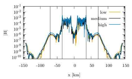
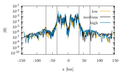
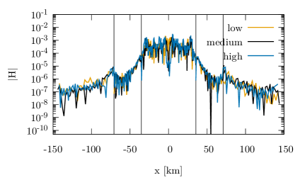
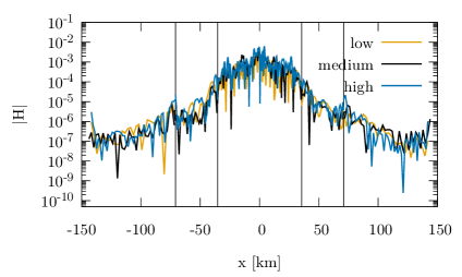
Figure 13: The Hamiltonian constraint along the $x$-axis scaled for $2^{\rm nd}$ order convergence for the runs with two 1.3 M_⊙ stars and the soft equation of state ($\Gamma=2.00$) at different times in the simulations. We have only plotted the three finest refinement levels and have indicated the boundaries between refinement levels with vertical thin lines. The top left plot is at $t=0.05$ ms, that is, shortly after the beginning of the simulation. The top right plot is at the $t=1.81$ ms (low resolution), $t=1.84$ ms (medium resolution) and $t=1.87$ ms (high resolution), when the neutron stars have returned to the $x$-axis after half an orbit. The bottom left plot is at $t=3.13$ ms (low resolution), $T=3.23$ ms (medium resolution) and $t=3.33$ ms (high resolution), when the stars have again returned to the $x$-axis after having completed a full orbit. The final bottom right plot is at a $t=13.1$ ms, that is, a time significantly after the merger.

4 Summary and outlook

In this paper, we have described the current status of our freshly developed general-relativistic, Lagrangian hydrodynamics code SPHINCS_BSSN. Since the focus of our original paper rosswog21a was to demonstrate the ability to accurately handle fully dynamical, general relativistic single stars, our main focus here is on those new methodological elements that are needed to simulate relativistic binary neutron star mergers. These elements include, in particular, a structured mesh (“fixed mesh refinement”; see Sec 2.1.2) on which we evolve the spacetime. This, in turn, requires improvements to the particle–mesh coupling, as explained in detail in Sec. 2.1.3. Finally, we describe a new method to accurately set up SPH particles based on the results from initial data solvers such as LORENE, see Sec. 2.2. The method is implemented in a new code called SPHINCS_ID.

Given the central role of Numerical Relativity for relativistic astrophysics and for gravitational wave astronomy, we consider this (to the best of our knowledge) first Lagrangian hydrodynamics approach that solves the full set of Einstein equations, as an important step forward. It will allow to validate both Eulerian Numerical Relativity approaches as well as Lagrangian ones that use only approximate strong-field gravity.

Despite this progress, it is clear that our current code version only contains the most basic physics ingredients, that is, relativistic hydrodynamics, dynamical evolution of the spacetime and simple equations of state. The first detection of a binary neutron star merger abbott17b ; abbott17c , however, has impressively underlined the multi-physics nature of neutron star merger events. It has demonstrated in particular that neutron star mergers are, as it had been expected for some time lattimer74 ; eichler89 ; rosswog99 ; freiburghaus99b , prolific sources of r-process elements kasen17 ; kasliwal17 ; tanvir17 ; rosswog18a . The detection of the early blue kilonova component evans17 and the identification of strontium watson19 , a very light r-process element that is only synthesized for moderately large electron fractions, have emphasized that weak interactions play a crucial role in shaping the observable features of a neutron star merger event. Moreover, the short GRB following GW170817 demonstrated that (at least some) neutron star mergers are able to launch relativistic jets. Taken together, these observations suggest that at least nuclear matter properties, neutrino physics and likely magnetic fields are major actors in a neutron star merger event.

Our next SPHINCS_BSSN development steps will be geared towards both further technical improvements and towards more realistic micro-physics. On the technical side, for example, we expect that the amount of dissipation that is applied in the hydrodynamic evolution can be further reduced and we aim at further increasing the code’s computational performance. In the current stage, both (artificial) dissipation and finite resolution likely still leave a noticeable imprint on the simulation outcome. On the micro-physical side, we consider the implementation of realistic nuclear matter equations of state as they are provided in the CompOSE database as an important and natural step forward. In addition to increasing the physical accuracy of the matter description, this ingredient is also indispensable to follow the electron fraction $Y_{e}$ of the ejecta and to implement (any kind of) neutrino physics. CompOSE equations of state can be used in LORENE but, in its present form, SPHINCS_BSSN does not yet support tabulated EOSs. The implementation of tabulated equations of state requires changes in the very core of our hydrodynamics scheme; in particular, we have to change the algorithm for the conversion from conserved to primitive variables. This has, of course, been successfully done in Eulerian contexts siegel18 ; kastaun21 , and is certainly also doable for our equation set, but it will require some dedicated effort. Once this has been achieved, we will tackle the implementation of a fast, yet reasonably accurate neutrino treatment such as the Advanced Spectral Leakage Scheme (ASL) perego16 ; gizzi19a ; gizzi21a . These issues will be addressed in future work.

Appendix A Gravitational wave extraction

At this early stage of our new code, we can extract gravitational waves in two different ways. We can either use the quadrupole approximation directly while the simulation is running or we can post process data afterwards using the Einstein Toolkit. In the following we describe both methods.

A.1 The quadrupole approximation

The “standard Einstein–Landau–Lifshitz quadrupole formula” misner73 ; blanchet90 reads

$$h_{ij}(t,\vec{x})=\frac{2G}{c^{4}r}P_{ijkl}(\vec{n})\frac{d^{2}}{dt^{2}}{\not{I}}_{kl}(t-r/c).$$ (54)

Here $P_{ijkl}$ is the transverse traceless projection operator

$$P_{ijkl}(\vec{n}) \equiv (\delta_{ik}-n_{i}n_{k})(\delta_{jl}-n_{j}n_{l})-$$ (56)

$$\frac{1}{2}(\delta_{ij}-n_{i}n_{j})(\delta_{kl}-n_{k}n_{l})$$

$$= P_{i}^{k}P_{j}^{l}-\frac{1}{2}P_{ij}P^{kl}$$ (57)

with $P_{i}^{k}=\delta_{i}^{k}-n_{i}n^{k}$, $r=|\vec{x}|=(\delta_{ij}x^{i}x^{j})^{1/2}$, $\vec{n}=\vec{x}/r$ and ${{\not{I}}}_{ij}=I_{jk}-\frac{1}{3}\delta_{ij}\sum_{k}I_{kk}$ is the reduced quadrupole moment. The amplitude becomes maximal, $h_{\rm max}$, for an observer located on the $z$-axis [Cartesian coordinates; see shibata16 , Eq. (1.47)]:

$$h_{\rm max}=\frac{G}{c^{4}}\frac{1}{D_{\rm obs}}\left(\ddot{I}_{xx}-\ddot{I}_{yy}\right),$$ (58)

where $D_{\rm obs}$ is the distance to the observer. The total energy radiated in gravitational waves is given by

$$E_{\rm GW} = \frac{1}{5}\frac{G}{c^{5}}\int_{-\infty}^{\infty}\dddot{{\not{I}}}_{ij}\dddot{{\not{I}}}_{ij}\;dt.$$ (59)

There is no unique way, in General Relativity, to define the quadrupole moment $I_{ij}$. One could try to follow post-Newtonian (PN) approaches, but they are sometimes ill-defined in the strong gravity regime and adding further PN-corrections does not necessarily improve the result. Shibata and Sekiguchi shibata03b find the quadrupole approximation rather useful even in strong-field gravity, they quote accuracies of $O(\mathcal{C})$ ($\mathcal{C}$ being the compactness) for the amplitudes, that is, in practice $\sim 20\%$, and much better accuracies for the phase evolutions.

Following blanchet90 ; shibata03b we calculate the quadrupole moment via the conserved rest-mass density,

$$\rho^{\ast}\equiv\sqrt{-g}\,U^{0}\rho_{\rm rest},$$ (60)

with the rest-mass density,

$$\rho_{\rm rest}=n\,m_{0}.$$ (61)

The quantity $\rho^{\ast}$ is related to our density variable $N$ (Eq. 7) by

$$\rho^{\ast}=m_{0}N.$$ (62)

The major advantage of this approach is that the first time derivative can be expressed analytically as

$$\frac{dI_{ij}}{dt}=\int d^{3}x\;\rho^{\ast}(v^{i}x^{j}+v^{j}x^{i}).$$ (63)

For the SPH representation, we transform the integral into a sum using the particles’ volume elements $V_{b}=\nu_{b}/N_{b}$,

$$\frac{dI_{ij}}{dt} = m_{0}\sum_{b}\nu_{b}(v^{i}_{b}x^{j}_{b}+v^{j}_{b}x^{i}_{b}).$$ (64)

To obtain the second and third time derivatives of $I_{ij}$, we monitor $dI_{ij}/dt$ at a set of instances in time, calculate a least square fit to them and take the analytical time derivatives of the approximating least square polynomial.

A.2 Extraction from the spacetime via the Einstein Toolkit

During the evolution we regularly write checkpoint files in order to be able to restart the simulation. There is one such checkpoint file for the particle (matter) data and another one for the grid (spacetime/BSSN) data. We have written a file reader that can read one complete refinement level of BSSN data from the checkpoint file into Cactus and thereby run the gravitational wave extraction tools available in the Einstein Toolkit. This consists of the thorns Extract, WeylScal 4 and Multipole. In Extract one, or several, extraction surfaces can be set up and the thorn will then estimate a suitable background metric and extract the Regge–Wheeler–Zerilli gauge invariant even $Q^{+}_{\ell m}$ and odd $Q^{\crossproduct}_{\ell m}$ parity master functions. Thorn WeylScal 4 calculates the Newman–Penrose Weyl scalar $\Psi_{4}$ everywhere on the grid. Thorn Multipole is then used to decompose $\Psi_{4}$ into spin-weighted spherical harmonics modes $\Psi_{4}^{\ell m}$ on a set of defined coordinate spheres.

Conveniently, alcubierre08 has collected all the necessary formulae for recovering the strain and to calculate the radiated energy and angular momentum (as well as linear momentum, but that is not needed here). For completeness we list these formulae here.

With the definition

$$P^{\crossproduct}_{\ell m}\coloneqq\int_{-\infty}^{t}Q^{\crossproduct}_{\ell m}dt^{\prime},$$ (65)

the strain can be recovered from $Q^{+}_{\ell m}$ and $P^{\crossproduct}_{\ell m}$ as

$$h^{+}+ih^{\crossproduct}=\frac{1}{\sqrt{2}r}\sum_{\ell,m}\left[Q^{+}_{\ell m}-iP^{\crossproduct}_{\ell m}\right]\prescript{}{-2}{Y}_{\ell m},$$ (66)

where $r$ is the distance from the source and $\prescript{}{-2}{Y}_{\ell m}$ is the spin-weight $-2$ spherical harmonic and the sum is over all possible $\ell$ and $m$. The radiated energy can be calculated as

$$\frac{dE}{dt}=\lim_{r\rightarrow\infty}\frac{1}{32\pi}\sum_{\ell,m}\left(\left|\dot{Q}^{+}_{\ell m}\right|^{2}+\left|Q^{\crossproduct}_{\ell m}\right|^{2}\right),$$ (67)

where a dot indicates the time derivative. The radiated angular momentum in the $z$-direction is

$$\frac{dJ_{z}}{dt}=\lim_{r\rightarrow\infty}\frac{i}{32\pi}\sum_{\ell,m}m\left(\bar{Q}^{+}_{\ell m}\dot{Q}^{+}_{\ell m}+\bar{P}^{\crossproduct}_{\ell m}Q^{\crossproduct}_{\ell m}\right),$$ (68)

where an overbar means a complex conjugate.

Starting from the $\Psi_{4}^{\ell m}$ modes, the strain can be recovered as

$$h^{+}+ih^{\crossproduct}=-\int_{-\infty}^{t}\int_{-\infty}^{t^{\prime}}\sum_{\ell,m}\Psi_{4}^{\ell m}\prescript{}{-2}{Y}_{\ell m}\,dt^{\prime\prime}\,dt^{\prime}.$$ (69)

The radiated energy can also be calculated from the $\Psi_{4}$ modes as

$$\frac{dE}{dt}=\lim_{r\rightarrow\infty}\frac{r^{2}}{16\pi}\sum_{\ell,m}\left|\int_{-\infty}^{t}\Psi_{4}^{\ell m}dt^{\prime}\right|^{2}$$ (70)

and the radiated $z$-component of the angular momentum as

$$\frac{dJ_{z}}{dt} = -\lim_{r\rightarrow\infty}\frac{ir^{2}}{16\pi}\imaginary\left[\sum_{\ell,m}m\int_{-\infty}^{t}\int_{-\infty}^{t^{\prime}}\Psi_{4}^{\ell m}\,dt^{\prime}\,dt^{\prime\prime}\right.$$ (71)

$$\left.\times\int_{-\infty}^{t}\bar{\Psi}_{4}^{\ell m}\right].$$

The analysis of the extracted modes from the Cactus simulation has been performed using kuibit Bozzola2021 .

Appendix B Details on the Artificial Pressure Method

B.1 The initial particle distribution on spherical surfaces

The aim is to find an as-good-as-possible representation of the LORENE density distribution by means of a finite number of (close to) equal-mass SPH particles. We start with a trial particle distribution and perform iterative APM improvements on it until an optimal configuration has been found. Obviously, the better the initial particle distribution, the fewer APM iterations will be needed to reach the final goal. We had experimented with placing particles on cubic lattices as initial positions, but starting from spherical surfaces delivered a) a slightly better density accuracy and b) resulted in a locally isotropic particle distribution while in the cubic lattice case preferred directions were still visible. Our method of choice therefore starts with particles placed on spherical surfaces and is described in more detail below.

We describe the method for one star only, since it is applied separately and independently for each star. First, we compute the “desired particle mass” as

$$m_{\mathrm{p}}=\dfrac{M_{\mathrm{b}}}{n_{\mathrm{des}}},$$ (72)

where $M_{\mathrm{b}}$ is the baryon mass of the star given by LORENE, and $n_{\mathrm{des}}$ “desired particle number” for the star, specified by the user. Second, we integrate the baryon mass density of the star $\rho_{\mathrm{b}}(r,\theta,\phi)$ given by LORENE, over $(r,\theta,\phi)$ and extract the radial baryon mass profile $M_{\mathrm{b}}(r)$. Notice that, since the star is not spherically symmetric, and we place particles on the spherical surfaces uniformly, we lose the density information over $(\theta,\phi)$ in this step. Third, in order to set the number of spherical surfaces inside the stars, we estimate the “radial particle profile” as

$$\mathrm{par}(r)\coloneqq\int_{0}^{r}\bigg{(}\dfrac{\rho_{\mathrm{b}}(\xi)}{m_{\mathrm{p}}}\bigg{)}^{1/3}\differential\xi,$$ (73)

Thus, we define the number of spherical surfaces as

$$n_{\mathrm{s}}\coloneqq\left\lceil\mathrm{par}(R)\right\rceil,$$ (74)

where $\left\lceil\cdot\right\rceil$ is the “ceiling” function, and $R$ the larger radius of the star—the equatorial radius on the $x$ axis towards the companion. Fourth, we need to set the radii of the spherical surfaces. We would like to have a larger density of surfaces where the baryon mass density is larger, and a lower density of surfaces where the baryon mass density is lower. Therefore, we place the first spherical surface at a radius given by

$$r_{1}=\left(\dfrac{\rho_{\mathrm{b}}^{\mathrm{center}}}{m_{\mathrm{p}}}\right)^{-1/3},$$ (75)

and the others at radii

$$r_{i}=r_{i-1}+\left(\dfrac{\rho_{\mathrm{b}}(r_{i-1})}{m_{\mathrm{p}}}\right)^{-1/3},\quad i\in\{2,...,n_{\mathrm{s}}\}.$$ (76)

The density in (76) is evaluated along the larger equatorial radius (i.e., along the $x$ axis in the direction of the companion). If, for some $i<n_{\mathrm{s}}$, $r_{i}$ falls outside of the star, we rescale all the radii by the same factor $i/n_{\mathrm{s}}<1$. It can still happen that the last surface falls outside of the star, hence we let the location of the last surface, $r_{\mathrm{last}}$, to be specified by the user. Note that this choice does affect how many particles are placed close to the surface and where. We found that placing the last surface at $r_{\mathrm{last}}\in[0.95R,0.99R]$ allows us to place enough particles close to the surface without allowing for very low-mass particles. Hence, when we know all the radii, we rescale them as

$$r_{i}\rightarrow\dfrac{r_{\mathrm{last}}}{r_{n_{\mathrm{s}}}}\,r_{i},$$ (77)

so that $r_{n_{\mathrm{s}}}\rightarrow r_{\mathrm{last}}$. At this point, we assign to each spherical surface a baryon mass given by

$$M_{i}=M_{\mathrm{b}}(r_{i})-M_{\mathrm{b}}(r_{i-1}),\quad i\in\{1,...,n_{\mathrm{s}}-1\}.$$ (78)

where $i$ is the surface index and $r_{0}=0$ (center of the star). For the last surface, the baryon mass is assigned as

$$M_{\mathrm{last}}=M_{\mathrm{b}}(R)-M_{\mathrm{b}}(r_{n_{\mathrm{s}}-1}),$$ (79)

In the last step, we place $n_{i}$ particles on each surface, where

$$n_{i}=\lfloor M_{i}/m_{\mathrm{p}}\rceil,$$ (80)

where $\lfloor x\rceil$ returns the nearest integer to $x$.

The particles are placed uniformly, avoiding their clustering around the poles, according to the algorithm described in weisstein . This consists of placing particles uniformly in the azimuth $\phi$ and $\nu$, with $\nu\in(0,1)$ and colatitude $\theta=\arccos(2\nu-1)$. We place the same number of particles on each meridian and each parallel, such that each quarter of meridian (parallel) contains the same number of particles. In other words, the number of particles $n_{\mathrm{circle}}$ on each meridian and parallel is a multiple of 4. Consider the part of a meridian spanned from $\theta=0$ to $\theta=\pi/2$. The number of particles on this curve is $n_{\mathrm{circle}}/4$ by construction. Then, the number of particles over the entire northern hemisphere is $n_{\mathrm{circle}}^{2}/4$. The total number of particles on the spherical surface is then

$$n_{\mathrm{s}}=\dfrac{n_{\mathrm{circle}}^{2}}{2}.$$ (81)

In practice, $n_{s}$ is set by (80), and $n_{\mathrm{circle}}$ is computed by inverting (81),

$$n_{\mathrm{circle}}=\lfloor\sqrt{2n_{\mathrm{s}}}\rceil.$$ (82)

Note that $n_{\mathrm{circle}}$ has to be a multiple of 4, so we correct it before using it. After correcting $n_{\mathrm{circle}}$, we consistently recompute $n_{\mathrm{s}}$ and place the particles at the desired positions, as described above. At each of these positions, we check that the LORENE mass density is positive, and we place a particle only if it is.

We highlight that this algorithm keeps the same mass for particles on the same surface, but due to the described rounding to integers, the particle mass changes a little between surfaces. In addition, for a spherical shell close to the surface of the star, some positions have a zero density since the star is not spherically symmetric. Such positions are not promoted to be particles, hence the final number of particles on the spherical surface changes (i.e., it is not $n_{\mathrm{s}}$ anymore). Thus, the particle mass on the spherical surface changes, since the mass of the surface in (78), (79) is kept the same. Since we would like to have (almost) equal mass particles, the change in particle mass between the surfaces should be small enough. To address this issue, we set up an iteration. The iteration replaces the particles on each surface, with the exception of the first surface considered, so that the particle mass on a surface is not too much different than the particle mass on the previous surface. The tolerance is specified by the user, and we found that a $2.5\%$ difference is reasonable.

Note that since we impose $n_{\mathrm{des}}^{\mathrm{star\,1}}/n_{\mathrm{des}}^{\mathrm{star\,2}}=M^{1}_{\mathrm{b}}/M^{2}_{\mathrm{b}}$, and since the particle number obtained at the end of the iteration is close to the desired particle number, the particle numbers on the stars will have a ratio very close to the binary mass ratio. Thus, the particle mass ratio across the stars will be similar to the particle mass ratio within each star, the latter being small thanks to the iteration on the spherical surfaces and, more importantly, to the APM iteration described in Sec. 2.2.2.

Finally, since the particles on spherical surfaces have very similar masses, it is well-justified to assume them to be equal-mass (assumption that the APM uses) and use them as initial condition for the APM iteration.

B.2 Placing ghost particles for BNS

We place the ghost particles on a cubic lattice around each star if two conditions are satisfied: the baryon mass density given by LORENE at that point is 0—so we are outside the star—and the position is between two ellipsoidal surfaces. The semi-axes of the innermost ellipsoidal surface are

$$\xi_{x} =R+\delta$$ (83a)

$$\xi_{y} =R_{y}+\delta$$ (83b)

$$\xi_{z} =R_{z}+\delta$$ (83c)

, with $R$ being the equatorial radius towards the companion, $R_{y}$, $R_{z}$ the radii in the $y$ and $z$ direction (given by LORENE), and series $\delta=0.3$km being a constant whose purpose is described next. The semi-axes of the innermost ellipsoidal surface are placed a little outside of the surface of the star—this is achieved by adding $\delta$ in (83)—to allow for the real particles to move towards the surface of the star if the artificial pressures of their neighbours push them there. If the ghost particles were placed exactly on the surface, then the real particles would not move towards it due to the high pressure gradient they would feel. The actual value of $\delta$ was determined empirically.

Appendix C Constraint violations and convergence for the BNS ID

After setting up the SPH and BSSN ID, we check that they satisfy the constraint equations using a subroutine from the Einstein Toolkit, which is adapted to our framework in SPHINCS_BSSN.

We compute the Hamiltonian and momentum constraints in two ways. First, using the full (spacetime and hydro) LORENE ID on the refined mesh, we compute the stress–energy tensor and finally the constraints. This method does not involve the SPH ID in any way. Second, we use the SPH ID on the particles and the BSSN ID on the refined mesh. We compute the stress–energy tensor at the particle positions, which needs the metric to be mapped to the particles (M2P step), and we map the stress–energy tensor to the refined mesh (P2M step). The interpolated stress–energy tensor on the mesh is then used together with the BSSN ID to compute the constraints. The two methods provide us also with another way to test the accuracy of the mapping routines.

We perform local convergence tests (alcubierre08, , Sec. 9.11) with the constraints computed in both ways, to test the robustness of our codes. Note that we do not recompute the entire ID with a different resolution when performing the convergence tests, since this is not possible in our framework. Even if we change the grid resolution, the LORENE spectral ID will stay the same; namely, it does not improve its accuracy. Hence, we expect to see convergence only if the finite error when computing spatial derivatives is larger than the error in the spectral solution from LORENE.

We found that keeping low finite difference order (FDO), and to a minor extent, keeping a low mesh resolution, is crucial to keep the finite differencing error larger than the spectral error. With FDO$=2$, we see convergence for some sequences of resolutions $\{\Delta$, $\Delta/r$, $\Delta/r^{2}\}$, with $r\in\{4/3,3/2,2\}$ (same resolution on each Cartesian axis). With FDO$=4,6$, the LORENE error dominates and it is harder to see convergence since the constraint violations change little, or not at all, when changing the resolution.

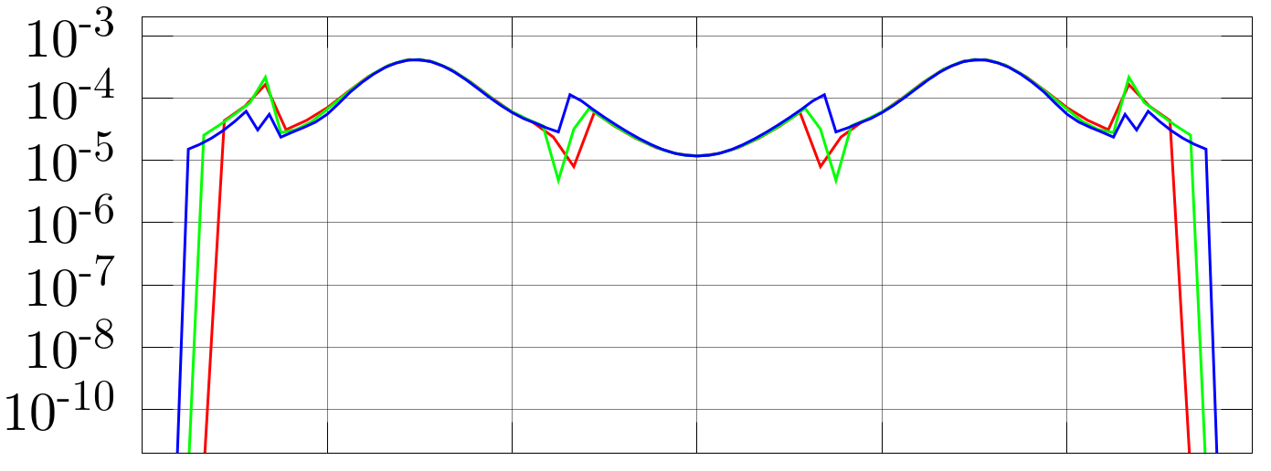
(a)

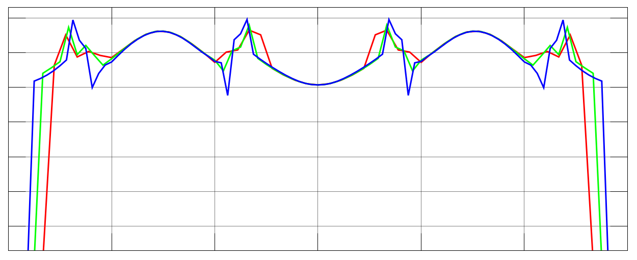
(b)

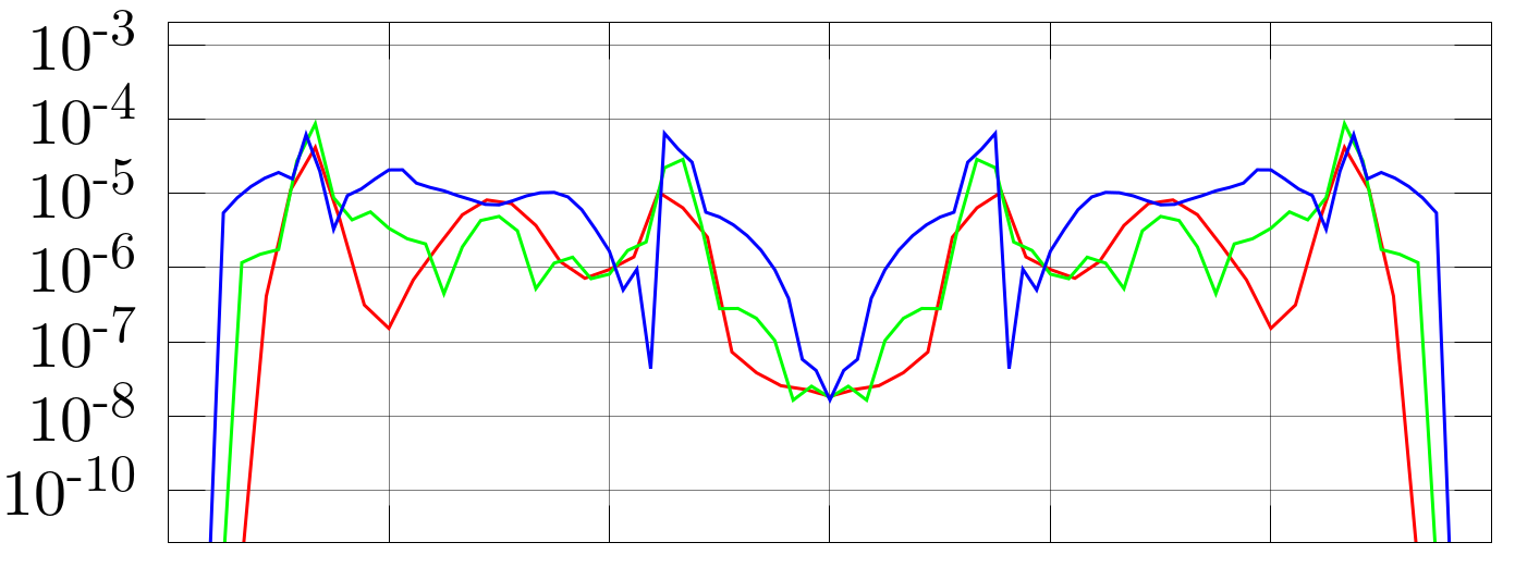
(c)

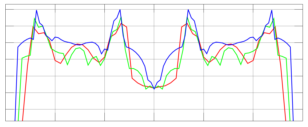
(d)

(e)

(f)

Figure 14: Rescaled absolute value of the Hamiltonian constraint violations on $x\in[-44.3,44.3]$km, computed using 3 different mesh resolutions. In the left panels, the full LORENE ID (spacetime and hydro) on the mesh (with one refinement level) is used; in the right panels, the computation uses the spacetime LORENE ID on the mesh (with one refinement level) and the stress–energy tensor computed at the particle positions and mapped to the mesh. The ID is the one for the run LR_2x1.3_G2.00. The coarse resolution (red) has $55^{3}$ grid points and $\Delta\simeq 1.64$km; the medium resolution (green) has $73^{3}$ grid points and $\Delta\simeq 1.23$km; the fine resolution (blue) has $97^{3}$ grid points and $\Delta\simeq 923$m. The ratio between the grid spacings is $4/3$, hence the Hamiltonian constraint violations on the medium resolution are divided by $(4/3)^{\rm FDO}$, and the one on the coarse resolution are divided by $(4/3)^{2\rm FDO}$. In the panels, from top to bottom, the FDO is $2$, $4$, $6$. The 3 rescaled Hamiltonian constraint violations in each panel should overlap to show convergence; this is seen only when FDO=2 since, for higher FDO, the error produced by LORENE is larger than the error produced by the finite difference approximation. Note that increasing the mesh resolution would decrease the finite differencing error too, the LORENE error would dominate, and there would be no convergence. Compared to the constraints violations computed using the ID on the mesh (left panels), those computed using the mapping (right panels) are larger at the surfaces of the stars, but comparable inside the stars. See text for more details. The lengths on the $x$ axis are given in units of the solar mass in geometrized units.

Figure 14 shows the rescaled absolute value of the Hamiltonian constraint violations on the $x$ axis for a sequence of resolutions with $r=4/3$, computed with the two methods described above, for the LR_2x1.3_G2.75 ID. In the examples shown in the figures, we see convergence only when FDO=2. Comparing the left and right panels of the figure, we note that the constraint violations are larger at the surfaces of the stars when mapping the metric from the mesh to the particles, and then the stress–energy tensor from the particles to the mesh, rather than just importing the LORENE ID on the mesh. This means that the error introduced by the mapping is a lot larger at the surfaces of the stars, compared to inside the stars. Specifically, in Figure 14, the mapping induces constraint violations of order between $10^{-4}$ and $10^{-3}$ at the surface of the star, irrespective of the FDO order and the mesh resolution. Lastly, even though we see convergence with FDO=2 only, it is evident from the figures that using a larger FDO leads to lower constraint violations.

- (1) B.P. Abbott, R. Abbott, T.D. Abbott, M.R. Abernathy, F. Acernese, K. Ackley, C. Adams, T. Adams, P. Addesso, R.X. Adhikari, et al., Physical Review Letters 116(6), 061102 (2016). DOI 10.1103/PhysRevLett.116.061102
- (2) B.P. Abbott, R. Abbott, T.D. Abbott, F. Acernese, K. Ackley, C. Adams, T. Adams, P. Addesso, R.X. Adhikari, V.B. Adya, et al., Nature 551, 85 (2017). DOI 10.1038/nature24471
- (3) B.P. Abbott, R. Abbott, T.D. Abbott, F. Acernese, K. Ackley, C. Adams, T. Adams, P. Addesso, R.X. Adhikari, V.B. Adya, et al., Physical Review Letters 119(16), 161101 (2017). DOI 10.1103/PhysRevLett.119.161101
- (4) B.P. Abbott, R. Abbott, T.D. Abbott, F. Acernese, K. Ackley, C. Adams, T. Adams, P. Addesso, R.X. Adhikari, V.B. Adya, et al., ApJL 848, L12 (2017). DOI 10.3847/2041-8213/aa91c9
- (5) B.P. Abbott, R. Abbott, T.D. Abbott, F. Acernese, K. Ackley, C. Adams, T. Adams, P. Addesso, R.X. Adhikari, V.B. Adya, et al., ApJL 848, L13 (2017). DOI 10.3847/2041-8213/aa920c
- (6) S.J. Smartt, T.W. Chen, A. Jerkstrand, M. Coughlin, E. Kankare, S.A. Sim, M. Fraser, C. Inserra, K. Maguire, K.C. Chambers, M.E. Huber, et al., Nature 551, 75 (2017). DOI 10.1038/nature24303
- (7) M. Tanaka, Y. Utsumi, P.A. Mazzali, N. Tominaga, M. Yoshida, Y. Sekiguchi, T. Morokuma, K. Motohara, K. Ohta, K.S. Kawabata, F. Abe, K. Aoki, Y. Asakura, S. Baar, S. Barway, I.A. Bond, M. Doi, T. Fujiyoshi, H. Furusawa, S. Honda, Y. Itoh, M. Kawabata, N. Kawai, J.H. Kim, C.H. Lee, S. Miyazaki, K. Morihana, H. Nagashima, T. Nagayama, T. Nakaoka, F. Nakata, R. Ohsawa, T. Ohshima, H. Okita, T. Saito, T. Sumi, A. Tajitsu, J. Takahashi, M. Takayama, Y. Tamura, I. Tanaka, T. Terai, P.J. Tristram, N. Yasuda, T. Zenko, Publications of the Astronomical Society of Japan 69(6), 102 (2017). DOI 10.1093/pasj/psx121
- (8) V.A. Villar, J. Guillochon, E. Berger, B.D. Metzger, P.S. Cowperthwaite, M. Nicholl, K.D. Alexander, P.K. Blanchard, R. Chornock, T. Eftekhari, W. Fong, R. Margutti, P.K.G. Williams, ApJL 851, L21 (2017). DOI 10.3847/2041-8213/aa9c84
- (9) M.M. Kasliwal, E. Nakar, L.P. Singer, D.L. Kaplan, et al., Science 358, 1559 (2017). DOI 10.1126/science.aap9455
- (10) A. Goldstein, P. Veres, E. Burns, M.S. Briggs, R. Hamburg, D. Kocevski, C.A. Wilson-Hodge, R.D. Preece, S. Poolakkil, O.J. Roberts, many more, ApJL 848, L14 (2017). DOI 10.3847/2041-8213/aa8f41
- (11) V. Savchenko, C. Ferrigno, E. Kuulkers, A. Bazzano, E. Bozzo, S. Brandt, J. Chenevez, T.J.L. Courvoisier, R. Diehl, A. Domingo, et al., ApJL 848(2), L15 (2017). DOI 10.3847/2041-8213/aa8f94
- (12) K.P. Mooley, A.T. Deller, O. Gottlieb, E. Nakar, G. Hallinan, S. Bourke, D.A. Frail, A. Horesh, A. Corsi, K. Hotokezaka, ArXiv e-prints (2018)
- (13) E.M.D. Symbalisty, D.N. Schramm, Astrophys. Lett. 22, 143 (1982)
- (14) D. Eichler, M. Livio, T. Piran, D.N. Schramm, Nature 340, 126 (1989)
- (15) S. Rosswog, M. Liebendörfer, F.K. Thielemann, M. Davies, W. Benz, T. Piran, A & A 341, 499 (1999)
- (16) C. Freiburghaus, S. Rosswog, F.K. Thielemann, ApJ 525, L121 (1999)
- (17) N.R. Tanvir, A.J. Levan, C. González-Fernández, O. Korobkin, I. Mandel, S. Rosswog, J. Hjorth, P. D’Avanzo, A.S. Fruchter, C.L. Fryer, T. Kangas, B. Milvang-Jensen, S. Rosetti, D. Steeghs, R.T. Wollaeger, Z. Cano, C.M. Copperwheat, S. Covino, V. D’Elia, A. de Ugarte Postigo, P.A. Evans, W.P. Even, S. Fairhurst, R. Figuera Jaimes, C.J. Fontes, Y.I. Fujii, J.P.U. Fynbo, B.P. Gompertz, J. Greiner, G. Hodosan, M.J. Irwin, P. Jakobsson, U.G. Jørgensen, D.A. Kann, J.D. Lyman, D. Malesani, R.G. McMahon, A. Melandri, P.T. O’Brien, J.P. Osborne, E. Palazzi, D.A. Perley, E. Pian, S. Piranomonte, M. Rabus, E. Rol, A. Rowlinson, S. Schulze, P. Sutton, C.C. Thöne, K. Ulaczyk, D. Watson, K. Wiersema, R.A.M.J. Wijers, ApJL 848, L27 (2017). DOI 10.3847/2041-8213/aa90b6
- (18) D. Kasen, B. Metzger, J. Barnes, E. Quataert, E. Ramirez-Ruiz, Nature 551, 80 (2017). DOI 10.1038/nature24453
- (19) J.J. Cowan, C. Sneden, J.E. Lawler, A. Aprahamian, M. Wiescher, K. Langanke, G. Martinez-Pinedo, F.K. Thielemann, Reviews of Modern Physics 93(1), 015002 (2021). DOI 10.1103/RevModPhys.93.015002
- (20) C.A. Raithel, F. Özel, D. Psaltis, Ap. J. Lett., 857(2), L23 (2018). DOI 10.3847/2041-8213/aabcbf
- (21) T. Malik, N. Alam, M. Fortin, C. Providência, B.K. Agrawal, T.K. Jha, B. Kumar, S.K. Patra, Phys. Rev. C.,98(3), 035804 (2018). DOI 10.1103/PhysRevC.98.035804
- (22) M. Shibata, K.ō. Uryū, Phys. Rev. D 61(6), 064001 (2000). DOI 10.1103/PhysRevD.61.064001
- (23) L. Baiotti, L. Rezzolla, Reports on Progress in Physics 80(9), 096901 (2017). DOI 10.1088/1361-6633/aa67bb
- (24) M. Shibata, S. Fujibayashi, K. Hotokezaka, K. Kiuchi, K. Kyutoku, Y. Sekiguchi, M. Tanaka, Phys. Rev. D.,96(12), 123012 (2017). DOI 10.1103/PhysRevD.96.123012
- (25) M. Shibata, K. Hotokezaka, Annual Review of Nuclear and Particle Science 69(1), annurev (2019). DOI 10.1146/annurev-nucl-101918-023625
- (26) D. Radice, S. Bernuzzi, A. Perego, Annual Review of Nuclear and Particle Science 70, 95 (2020). DOI 10.1146/annurev-nucl-013120-114541
- (27) M. Alcubierre, Introduction to 3+1 Numerical Relativity (Oxford University Press, 2008)
- (28) T.W. Baumgarte, S.L. Shapiro, Numerical Relativity: Solving Einstein’s Equations on the Computer (Cambridge, 2010)
- (29) L. Rezzolla, O. Zanotti, Relativistic Hydrodynamics (2013)
- (30) M. Shibata, K. Kiuchi, Y.i. Sekiguchi, Phys. Rev. D 95(8), 083005 (2017). DOI 10.1103/PhysRevD.95.083005
- (31) S. Rosswog, P. Diener, Classical and Quantum Gravity 38(11), 115002 (2021). DOI 10.1088/1361-6382/abee65
- (32) E. Gourgoulhon, P. Grandclement, K. Taniguchi, J.A. Marck, S. Bonazzola, Phys. Rev. D 63, 064029 (2001). DOI 10.1103/PhysRevD.63.064029
- (33) E. Gourgoulhon, P. Grandclement, J.A. Marck, J. Novak, K. Taniguchi, ascl:1608.018 (2016)
- (34) URL http://lorene.obspm.fr
- (35) M. Shibata, T. Nakamura, Phys. Rev. D 52, 5428 (1995). DOI 10.1103/PhysRevD.52.5428
- (36) T.W. Baumgarte, S.L. Shapiro, Phys. Rev. D 59(2), 024007 (1999). DOI 10.1103/PhysRevD.59.024007
- (37) J.J. Monaghan, Reports on Progress in Physics 68, 1703 (2005)
- (38) S. Rosswog, New Astronomy Reviews 53, 78 (2009)
- (39) D.J. Price, Journal of Computational Physics 231, 759 (2012). DOI 10.1016/j.jcp.2010.12.011
- (40) S. Rosswog, MNRAS 448, 3628 (2015). DOI 10.1093/mnras/stv225
- (41) S. Rosswog, M.B. Davies, MNRAS 334, 481 (2002). DOI 10.1046/j.1365-8711.2002.05409.x
- (42) W.H. Lee, E. Ramirez-Ruiz, G. van de Ven, ApJ 720, 953 (2010). DOI 10.1088/0004-637X/720/1/953
- (43) S. Ayal, M. Livio, T. Piran, ApJ 545, 772 (2000). DOI 10.1086/317835
- (44) J.A. Faber, F.A. Rasio, Phys. Rev. D 62(6), 064012 (2000)
- (45) J.A. Faber, F.A. Rasio, J.B. Manor, Phys. Rev. D 63(4), 044012 (2001). DOI 10.1103/PhysRevD.63.044012
- (46) L. Blanchet, T. Damour, G. Schaefer, MNRAS 242, 289 (1990)
- (47) P. Laguna, W.A. Miller, W.H. Zurek, ApJ 404, 678 (1993). DOI 10.1086/172321
- (48) D. Liptai, D.J. Price, MNRAS 485(1), 819 (2019). DOI 10.1093/mnras/stz111
- (49) R. Oechslin, S. Rosswog, F.K. Thielemann, Phys. Rev. D 65(10), 103005 (2002)
- (50) A. Bauswein, H. Janka, R. Oechslin, G. Pagliara, I. Sagert, J. Schaffner-Bielich, M.M. Hohle, R. Neuhäuser, Physical Review Letters 103(1), 011101 (2009). DOI 10.1103/PhysRevLett.103.011101
- (51) J. Isenberg, preprint University of Maryland; unpublished but available as http://arxiv.org/abs/gr-qc/0702113; (1978)
- (52) J.R. Wilson, G.J. Mathews, Physical Review Letters 75, 4161 (1995). DOI 10.1103/PhysRevLett.75.4161
- (53) S. Rosswog, MNRAS 498(3), 4230 (2020). DOI 10.1093/mnras/staa2591
- (54) S. Diot, R. Loubere, S. Clain, International Journal for Numerical Methods in Fluids 73, 362 (2013)
- (55) M. Shibata, Numerical Relativity (2016). DOI 10.1142/9692
- (56) D. Garcia-Senz, R. Cabezon, J. Escartin, A & A 538, A9 (2012). DOI 10.1051/0004-6361/201117939
- (57) J. von Neumann, R.D. Richtmyer, Journal of Applied Physics 21, 232 (1950)
- (58) N. Frontiere, C.D. Raskin, J.M. Owen, Journal of Computational Physics 332, 160 (2017). DOI 10.1016/j.jcp.2016.12.004
- (59) J. Morris, J. Monaghan, J. Comp. Phys. 136, 41 (1997)
- (60) S. Rosswog, M.B. Davies, F.K. Thielemann, T. Piran, A&A 360, 171 (2000)
- (61) L. Cullen, W. Dehnen, MNRAS 408, 669 (2010). DOI 10.1111/j.1365-2966.2010.17158.x
- (62) S. Rosswog, ApJ 898(1), 60 (2020). DOI 10.3847/1538-4357/ab9a2e
- (63) H. Wendland, Advances in Computational Mathematics 4, 389 (1995)
- (64) E. Gafton, S. Rosswog, MNRAS 418, 770 (2011). DOI 10.1111/j.1365-2966.2011.19528.x
- (65) P. Marronetti, W. Tichy, B. Brügmann, J. Gonzalez, U. Sperhake, Phys. Rev. D 77(6), 064010 (2008). DOI 10.1103/PhysRevD.77.064010
- (66) W. Tichy, P. Marronetti, Phys. Rev. D 76(6), 061502 (2007). DOI 10.1103/PhysRevD.76.061502
- (67) J.D. Brown, P. Diener, O. Sarbach, E. Schnetter, M. Tiglio, Phys. Rev. D 79, 044023 (2009). DOI 10.1103/PhysRevD.79.044023
- (68) Einstein Toolkit web page. https://einsteintoolkit.org/ (2020). [Online; accessed 9-December-2020]
- (69) F. Löffler, J. Faber, E. Bentivegna, T. Bode, P. Diener, R. Haas, I. Hinder, B.C. Mundim, C.D. Ott, E. Schnetter, G. Allen, M. Campanelli, P. Laguna, Classical and Quantum Gravity 29(11), 115001 (2012). DOI 10.1088/0264-9381/29/11/115001
- (70) T.W. Baumgarte, S.L. Shapiro, Numerical Relativity (Cambridge, 2021)
- (71) S. Gottlieb, C.W. Shu, Mathematics of Computation 67, 73 (1998)
- (72) G.H. Cottet, P.D. Koumoutsakos, Vortex Methods (2000)
- (73) J.J. Monaghan, Ann. Rev. Astron. Astrophys. 30, 543 (1992)
- (74) G. Cottet, J. Etancelin, F. Perignon, C. Picard, ESAIM: Mathematical Modelling and Numerical Analysis, EDP Sciences 48, 1029 (2014). DOI 10.1086/185939
- (75) É. Gourgoulhon, 3+1 Formalism in General Relativity: Bases of Numerical Relativity. Lecture Notes in Physics (Springer Berlin Heidelberg, 2012). URL https://books.google.se/books?id=XwB94Je8nnIC
- (76) L. Bildsten, C. Cutler, ApJ 400, 175 (1992). DOI 10.1086/171983
- (77) C.S. Kochanek, ApJ 398, 234 (1992). DOI 10.1086/171851
- (78) S. Bernuzzi, T. Dietrich, W. Tichy, B. Brügmann, Phys. Rev. D.,89(10), 104021 (2014). DOI 10.1103/PhysRevD.89.104021
- (79) T. Dietrich, N. Moldenhauer, N.K. Johnson-McDaniel, S. Bernuzzi, C.M. Markakis, B. Brügmann, W. Tichy, Phys. Rev. D 92(12), 124007 (2015). DOI 10.1103/PhysRevD.92.124007
- (80) R. Dudi, T. Dietrich, A. Rashti, B. Bruegmann, J. Steinhoff, W. Tichy, arXiv e-prints arXiv:2108.10429 (2021)
- (81) Compstar online supernova equations of state. https://compose.obspm.fr
- (82) S. Diehl, G. Rockefeller, C.L. Fryer, D. Riethmiller, T.S. Statler, Publications of the Astronomical Society of Australia 32, e048 (2015). DOI 10.1017/pasa.2015.50
- (83) Alexander Arth, Julius Donnert, Ulrich Steinwandel, Ludwig Böss, Timo Halbesma, Martin Pütz, David Hubber, Klaus Dolag, CoRR (2019)
- (84) S. Rosswog, Living Reviews of Computational Astrophysics (2015) 1 (2015). DOI 10
- (85) E. Gaburov, K. Nitadori, MNRAS 414, 129 (2011). DOI 10.1111/j.1365-2966.2011.18313.x
- (86) C. Misner, K. Thorne, J. Wheeler, Gravitation (Freeman, New York, 1973)
- (87) J.A. Font, T. Goodale, S. Iyer, M. Miller, L. Rezzolla, E. Seidel, N. Stergioulas, W.M. Suen, M. Tobias, Phys. Rev. D 65, 084024 (2002). DOI 10.1103/PhysRevD.65.084024. URL https://link.aps.org/doi/10.1103/PhysRevD.65.084024
- (88) I. Cordero-Carrión, P. Cerdá-Durán, H. Dimmelmeier, J.L. Jaramillo, J. Novak, E. Gourgoulhon, Phys. Rev. D.,79(2), 024017 (2009). DOI 10.1103/PhysRevD.79.024017
- (89) S. Bernuzzi, D. Hilditch, Phys. Rev. D 81(8), 084003 (2010). DOI 10.1103/PhysRevD.81.084003
- (90) T. Damour, A. Nagar, Phys. Rev. D.,80(8), 084035 (2009). DOI 10.1103/PhysRevD.80.084035
- (91) K. Hotokezaka, K. Kyutoku, H. Okawa, M. Shibata, K. Kiuchi, Phys. Rev. D 83(12), 124008 (2011). DOI 10.1103/PhysRevD.83.124008
- (92) A. Bauswein, T.W. Baumgarte, H.T. Janka, Physical Review Letters 111(13), 131101 (2013). DOI 10.1103/PhysRevLett.111.131101
- (93) S. Köppel, L. Bovard, L. Rezzolla, Ap. J. Lett., 872(1), L16 (2019). DOI 10.3847/2041-8213/ab0210
- (94) R. Kashyap, A. Das, D. Radice, S. Padamata, A. Prakash, D. Logoteta, A. Perego, D.A. Godzieba, S. Bernuzzi, I. Bombaci, F.J. Fattoyev, B.T. Reed, A. da Silva Schneider, arXiv e-prints arXiv:2111.05183 (2021)
- (95) F. Zappa, S. Bernuzzi, D. Radice, A. Perego, T. Dietrich, Phys. Rev. Lett. 120, 111101 (2018). DOI 10.1103/PhysRevLett.120.111101. URL https://link.aps.org/doi/10.1103/PhysRevLett.120.111101
- (96) L. Baiotti, S. Bernuzzi, G. Corvino, R. De Pietri, A. Nagar, Phys. Rev. D 79, 024002 (2009). DOI 10.1103/PhysRevD.79.024002. URL https://link.aps.org/doi/10.1103/PhysRevD.79.024002
- (97) D. Price, S. Rosswog, Science 312, 719 (2006)
- (98) K. Kiuchi, K. Kyutoku, Y. Sekiguchi, M. Shibata, T. Wada, Phys. Rev. D 90(4), 041502 (2014). DOI 10.1103/PhysRevD.90.041502
- (99) K. Kiuchi, P. Cerdá-Durán, K. Kyutoku, Y. Sekiguchi, M. Shibata, Phys. Rev. D 92(12), 124034 (2015). DOI 10.1103/PhysRevD.92.124034
- (100) K. Kiuchi, K. Kyutoku, Y. Sekiguchi, M. Shibata, Phys. Rev. D.,97(12), 124039 (2018). DOI 10.1103/PhysRevD.97.124039
- (101) O. Agertz, B. Moore, J. Stadel, D. Potter, F. Miniati, J. Read, L. Mayer, A. Gawryszczak, A. Kravtsov, Å. Nordlund, F. Pearce, V. Quilis, D. Rudd, V. Springel, J. Stone, E. Tasker, R. Teyssier, J. Wadsley, R. Walder, MNRAS 380, 963 (2007). DOI 10.1111/j.1365-2966.2007.12183.x
- (102) C.P. McNally, W. Lyra, J.C. Passy, ApJS 201, 18 (2012). DOI 10.1088/0067-0049/201/2/18
- (103) D. Radice, S. Bernuzzi, C.D. Ott, Phys. Rev. D.,94(6), 064011 (2016). DOI 10.1103/PhysRevD.94.064011
- (104) H. Müller, B.D. Serot, Nuc. Phys. A 606, 508 (1996). DOI 10.1016/0375-9474(96)00187-X
- (105) F. Douchin, P. Haensel, Astron. & Astrophys., 380, 151 (2001). DOI 10.1051/0004-6361:20011402
- (106) J.M. Lattimer, D.N. Schramm, ApJ, (Letters) 192, L145 (1974)
- (107) S. Rosswog, J. Sollerman, U. Feindt, A. Goobar, O. Korobkin, R. Wollaeger, C. Fremling, M.M. Kasliwal, A&A 615, A132 (2018). DOI 10.1051/0004-6361/201732117
- (108) P.A. Evans, S.B. Cenko, J.A. Kennea, S.W.K. Emery, N.P.M. Kuin, O. Korobkin, R.T. Wollaeger, C.L. Fryer, K.K. Madsen, F.A. Harrison, Y. Xu, E. Nakar, K. Hotokezaka, A. Lien, S. Campana, S.R. Oates, E. Troja, A.A. Breeveld, F.E. Marshall, S.D. Barthelmy, A.P. Beardmore, D.N. Burrows, G. Cusumano, A. D’Ai, P. D’Avanzo, V. D’Elia, M. de Pasquale, W.P. Even, C.J. Fontes, K. Forster, J. Garcia, P. Giommi, B. Grefenstette, C. Gronwall, D.H. Hartmann, M. Heida, A.L. Hungerford, M.M. Kasliwal, H.A. Krimm, A.J. Levan, D. Malesani, A. Melandri, H. Miyasaka, J.A. Nousek, P.T. O’Brien, J.P. Osborne, C. Pagani, K.L. Page, D.M. Palmer, M. Perri, S. Pike, J.L. Racusin, S. Rosswog, M.H. Siegel, T. Sakamoto, B. Sbarufatti, G. Tagliaferri, N.R. Tanvir, A. Tohuvavohu, Science 358, 1565 (2017). DOI 10.1126/science.aap9580
- (109) D. Watson, C.J. Hansen, J. Selsing, A. Koch, D.B. Malesani, A.C. Andersen, J.P.U. Fynbo, A. Arcones, A. Bauswein, S. Covino, A. Grado, K.E. Heintz, L. Hunt, C. Kouveliotou, G. Leloudas, A.J. Levan, P. Mazzali, E. Pian, Nature 574(7779), 497 (2019). DOI 10.1038/s41586-019-1676-3
- (110) D.M. Siegel, B.D. Metzger, ApJ 858(1), 52 (2018). DOI 10.3847/1538-4357/aabaec
- (111) W. Kastaun, J.V. Kalinani, R. Ciolfi, Phys. Rev. D.,103(2), 023018 (2021). DOI 10.1103/PhysRevD.103.023018
- (112) A. Perego, R.M. Cabezón, R. Käppeli, ApJS 223(2), 22 (2016). DOI 10.3847/0067-0049/223/2/22
- (113) D. Gizzi, E. O’Connor, S. Rosswog, A. Perego, R.M. Cabezon, L. Nativi, MNRAS 490(3), 4211 (2019). DOI 10.1093/mnras/stz2911
- (114) D. Gizzi, C. Lundman, E. O’Connor, S. Rosswog, A. Perego, Mon. not. RAS., 505(2), 2575 (2021). DOI 10.1093/mnras/stab1432
- (115) M. Shibata, Y.I. Sekiguchi, Phys. Rev. D.,68(10), 104020 (2003). DOI 10.1103/PhysRevD.68.104020
- (116) G. Bozzola, Journal of Open Source Software 6(60), 3099 (2021). DOI 10.21105/joss.03099. URL https://doi.org/10.21105/joss.03099
- (117) E.W. Weisstein. Sphere point picking. URL https://mathworld.wolfram.com/SpherePointPicking.html