Towards parallel time-stepping for the numerical simulation of atherosclerotic plaque growth

Abstract

The numerical simulation of atherosclerotic plaque growth is computationally prohibitive, since it involves a complex cardiovascular fluid-structure interaction (FSI) problem with a characteristic time scale of milliseconds to seconds, as well as a plaque growth process governed by reaction-diffusion equations, which takes place over several months. In this work we combine a temporal homogenization approach, which separates the problem in computationally expensive FSI problems on a micro scale and a reaction-diffusion problem on the macro scale, with parallel time-stepping algorithms. It has been found in the literature that parallel time-stepping algorithms do not perform well when applied directly to the FSI problem. To circumvent this problem, a parareal algorithm is applied on the macro-scale reaction-diffusion problem instead of the micro-scale FSI problem. We investigate modifications in the coarse propagator of the parareal algorithm, in order to further reduce the number of costly micro problems to be solved. The approaches are tested in detailed numerical investigations based on serial simulations.

1 Introduction

Cardiovascular diseases are by far the most common cause of death in industrialized nations today. One of the most common cardiovascular diseases is the growth of plaque (atherogenesis) in coronary arteries or the pathological accumulation of plaque (atherosclerosis), which can result in heart attacks or strokes that are often fatal. Since the formation of plaque ranges over a long period of time, from months to several years, early diagnosis and treatment to prevent plaque growth can have a good chance of success.

An important driving force for plaque growth is the wall shear stress distribution, which varies significantly within each heartbeat, i.e., every second; see, for instance, [57, 20] for a discussion on the dependence of plaque growth on the wall shear stress. Using three-dimensional fluid-structure interaction (FSI) simulations with realistic material models, the heartbeat scale has to be resolved by time steps in the order of milliseconds. We refer to [6, 5] for the first studies on using complex wall models that take into account the effect of the reinforcing fibers within three-dimensional FSI simulations. For further references on FSI for cardiovascular applications, see, e.g., [26, 9, 10, 38, 40]; for FSI simulations in the context of plaque growth, see also [25, 60, 30, 56, 46, 28].

Hence, realistic numerical simulations of plaque growth over several months that resolve each individual heartbeat would easily require $\mathcal{O}(10^{9})$ sequential time steps. Consequently, even using today’s fastest supercomputers, such a simulation is clearly infeasible.

Therefore, in [29] a temporal homogenization approach for separating the plaque growth time scale (macro scale) in the order of days and the FSI time scale (micro scale) in the order of milliseconds has been introduced. The approach is based on the assumption that the FSI is approximately periodic in time on the micro scale, which makes it possible to upscale the fluid dynamics to the macro scale. Using this approach it is possible to simulate only a moderate number of FSI time steps for each time step of the plaque growth problem. This means that we have to simulate only a few heartbeats (seconds) of the full FSI problem instead of the whole 24 hours of each day; the total number of time steps is reduced by a factor of $\mathcal{O}(10^{4})$. Note that, completely neglecting the fine scale may introduce a significant error; see [30, 28]. See also the recent PhD thesis of Florian Sonner for further details on temporal homogenization for plaque growth [55].

However, considering realistic three-dimensional simulations the number of time steps corresponding to fine scale FSI problems remains still infeasibly high, even after temporal homogenization. In order to further reduce the computational times, we introduce a new approach based on parallel time-stepping. We focus on a classical parallel time-stepping method, the parareal algorithm, which has been introduced by Lions et al. in [42]; for an overview over the vast literature on parallel-in-time integration methods, we refer to the review papers [31, 45] and the references therein.

Due to a phase-shift in a coarse solution for hyperbolic partial differential equations (PDEs), such as the structural problem in FSI, it is generally challenging to apply parallel time-stepping methods to FSI problems; see, e.g., [43, 51]. Thus, instead of applying the parareal algorithm to the micro-scale FSI problem, we apply it to the homogenized plaque growth problem on the macro scale. Plaque growth is typically modeled by a system of reaction-diffusion equations; see, e.g., [59, 54]. Instead of being hyperbolic, they have a parabolic character and hence can be solved more efficiently by parallel time-stepping methods.

The focus of this paper is not the computation of accurate plaque-growth predictions in patient-specific geometries. Instead, our objective is to introduce a numerical framework for making the simulation times feasible and to investigate the methods numerically. Therefore, we make several simplifications: We focus on two-dimensional FSI simulations on a simple geometry. Furthermore, we consider two simplified models for the plaque growth, that is, the ordinary differential equation (ODE) model already considered in [29, 28] as well as a more complex partial differential equation (PDE) of reaction-diffusion type. We formulate the parareal algorithm for the two-scale problem of plaque growth and also propose variants to increase the efficiency of the coarse-scale propagators. Finally, we investigate the parallel time-stepping methods numerically based on serial simulations. As, even in two dimensions, the micro-scale FSI problems are generally much more expensive than the coarse plaque growth problem, we are able to give some good estimates for the speedup that can be expected in fully parallel simulations.

The paper is structured as follows: In section 2, we introduce our fluid-structure interaction problem as well as the two solid growth models considered for modeling the plaque growth: an ODE-based model in section 2.2.1 and a reaction-diffusion equation-based model in section 2.2.2. Next, in section 3, we briefly introduce the variational formulation of the FSI problem and then describe the temporal homogenization approach including some first numerical results. In section 4, we recap the parareal algorithm and discuss how we estimate the computational costs and the possible speed up in parallel simulations. We also discuss numerical results for the parallel time-stepping approach using the simple ODE plaque growth model. Furthermore, we introduce some ideas for reducing the costs of the coarse-scale propagators. In section 5, we show results for the reaction-diffusion plaque growth model, including a theoretical discussion on the computational costs of the algorithms. We conclude in section 6, where we also give a brief outlook on topics for future work.

2 Model equations

We consider a time-dependent fluid-structure interaction system, where the fluid is modeled by the Navier–Stokes equations and the solid by the Saint Venant–Kirchhoff model. In order to account for the solid growth, we add a multiplicative growth term to the deformation gradient, which is motivated by typical plaque growth models [59, 30, 44, 54].

2.1 Fluid-structure interaction

Consider a partition of an overall domain $\Omega(t)={\cal F}(t)\cup\Gamma(t)\cup{\cal S}(t)$ into a fluid part ${\cal F}(t)$, an interface $\Gamma(t)$ and a solid part ${\cal S}(t)$. The blood flow and its interaction with the surrounding vessel wall is modelled by the following FSI system:

$$\rho_{f}(\partial_{t}\mathbf{v}_{f}+\mathbf{v}_{f}\cdot\nabla\mathbf{v}_{f})-\operatorname{div}\,\boldsymbol{\sigma}_{f} =0, \qquad\operatorname{div}\,\mathbf{v}_{f} =0\qquad\text{ in }{\cal F}(t),$$ (1)

$$\rho_{s}\partial_{t}\hat{\mathbf{v}}_{s}-\operatorname{div}\,(\hat{\mathbf{F}}_{e}\hat{\boldsymbol{\Sigma}}_{e}) =0, \qquad\partial_{t}\hat{\mathbf{u}}_{s}-\hat{\mathbf{v}}_{s} =0\qquad\text{ in }\hat{S},$$

$$\boldsymbol{\sigma}_{f}\vec{n}_{f}+\boldsymbol{\sigma}_{s}\vec{n}_{s} =0, \qquad\mathbf{v}_{f} =\mathbf{v}_{s}\quad\;\;\text{ on }\Gamma(t).$$

Here, $\mathbf{v}_{f}$ and $\hat{\mathbf{v}}_{s}$ denote the fluid and solid velocity, respectively, and $\hat{\mathbf{u}}_{s}$ the solid displacement. Quantities with a “hat” are defined in Lagrangian coordinates, while quantities without a “hat” are defined in the current Eulerian coordinate framework. Two quantities $\hat{f}(\hat{x})$ and $f(x)$ correspond to each other by a $C^{1,1}$-diffeomorphism $\hat{\xi}:\hat{\Omega}\to\Omega(t)$ and the relation $\hat{f}=f\circ\hat{\xi}$. Later, we will also need the solid deformation gradient $\hat{F}_{s}=I+\hat{\nabla}\hat{u}_{s}$, which is the derivative of $\hat{\xi}$ in the solid part. The constants $\rho_{f}$ and $\rho_{s}$ are the densities of blood and vessel wall, and $\vec{n}_{f}$ and $\vec{n}_{s}$ are outward pointing normal vectors of the fluid and solid domain, respectively.

By $\boldsymbol{\sigma}_{f}$ and $\boldsymbol{\sigma}_{s}$ we denote the Cauchy stress tensors of fluid and solid. Using the well-known Piola transformation between the Eulerian and the Lagrangian coordinate systems, we can relate $\boldsymbol{\sigma}_{s}$ and the second Piola–Kirchhoff stress $\hat{\Sigma}_{e}$ as follows:

$$\boldsymbol{\sigma}_{s}(x)=\hat{\boldsymbol{\sigma}}_{s}(\hat{x})=\hat{J}_{e}^{-1}\hat{\mathbf{F}}_{e}\hat{\boldsymbol{\Sigma}}_{e}(\hat{x})\hat{\mathbf{F}}_{e}^{T},$$

where $\hat{F}_{e}$ is the elastic part of the deformation gradient $\hat{F}_{s}$, For modeling the material behavior of the vessel wall, different approaches have been proposed and investigated in literature; see, e.g., [5, 8, 13, 7, 37] for more sophisticated material models, for instance, incorporating an anisotropic behavior due to the reinforcing fibers. For the sake of simplicity, we use in this work the relatively simple Saint Venant-Kirchhoff model with the Lamé material parameters $\mu_{s}$ and $\lambda_{s}$

$$\hat{\boldsymbol{\Sigma}}_{e}=2\mu_{s}\hat{\mathbf{E}}_{e}+\lambda_{s}\operatorname{tr}(\hat{\mathbf{E}}_{e})I,\quad\hat{\mathbf{E}}_{e}:=\frac{1}{2}(\hat{\mathbf{F}}_{e}^{T}\hat{\mathbf{F}}_{e}-I).$$ (2)

The Saint Venant-Kirchhoff model is based on Hooke’s linear material law in a large strain formulation, resulting in a weakly nonlinear material model.

The blood flow is modeled as an incompressible Newtonian fluid, such that the Cauchy stresses are given by

$$\boldsymbol{\sigma}_{f}=\rho_{f}\nu_{f}(\nabla\mathbf{v}_{f}+\nabla\mathbf{v}_{f}^{T})-p_{f}I,$$ (3)

where $\nu_{f}$ is the kinematic viscosity of blood. A sketch of the computational domain is given in fig. 1. We split the outer boundary of $\Omega$ into a solid part $\Gamma_{s}$ with homogeneous Dirichlet conditions, a fluid part $\Gamma^{\text{in}}_{f}$ with an inflow Dirichlet condition and an outflow part $\Gamma^{\text{out}}_{f}$, where a do-nothing condition is imposed.

The boundary data is given by

$$\mathbf{v}_{f}=\mathbf{v}^{\text{in}}\,\text{ on }\Gamma^{\text{in}}_{f},\quad\rho_{f}\nu_{f}(\vec{n}_{f}\cdot\nabla)\mathbf{v}_{f}-p_{f}\vec{n}_{f}=0 \,\text{ on }\Gamma^{\text{out}}_{f},\quad\hat{\mathbf{u}}_{s}=0\,\text{ on }\hat{\Gamma}_{s},$$ (4)

where $\mathbf{v}^{\text{in}}$ is the inflow velocity on $\Gamma^{\text{in}}_{f}$.

Figure 1: Sketch of the computational domain centered at the origin $(0,0)$; ${\cal F}$ and ${\cal S}$ are the fluid and solid parts, respectively, and the solid lines correspond to the fluid-solid interface $\Gamma$. The plaque growth is initiated at $(0,\pm 1)$.

2.2 Modelling of solid growth

Developing a realistic model of plaque growth at the vessel wall is a complex task that involves the interaction of many different molecules and species, see for example [54]. Furthermore, the plaque growth will also strongly depend on the geometry and material model of the arterial wall. In this contribution, our focus does not lie on a realistic modeling of plaque growth, and thus, our model is greatly simplified. However, the two models considered here are chosen to behave similarly (from a numerical viewpoint) to more sophisticated models. We consider a simple ODE-based model in section 2.2.1 and a more complex but still relatively simple PDE model of reaction-diffusion type in section 2.2.2. Both models focus on the influence of the concentration of foam cells $c_{s}$ on the growth. Numerical results can be found in sections 3.2, 4.1.4 and 4.2 as well as in section 5, respectively.

2.2.1 A simple ODE model for solid growth

In the first model, which is taken from [30, 28], the evolution of the foam cell concentration $c_{s}$ depends only on its current value but not on its spatial distribution. Hence, it can be described by a simple ODE. The rate of formation of these cells depends on the distribution of the wall shear stress $\boldsymbol{\sigma}_{f}^{WS}$ at the vessel wall. As a result, we obtain the following simplified ODE model:

$$\partial_{t}c_{s} =\gamma(\boldsymbol{\sigma}_{f}^{WS},c_{s})\coloneqq\alpha\big{(}1+c_{s}\big{)}^{-1}\left(1+\frac{\left\|\boldsymbol{\sigma}_{f}^{WS}\right\|_{L^{2}(\Gamma)}^{2}}{\sigma_{0}^{2}}\right)^{-1},$$ (5)

$$\boldsymbol{\sigma}_{f}^{WS} \coloneqq\rho\nu\big{(}I_{d}-\vec{n}_{f}\vec{n}_{f}^{T}\big{)}(\nabla\mathbf{v}+\nabla\mathbf{v}^{T})\vec{n}_{f}.$$

The reference wall shear stress $\sigma_{0}$ and the scale separation parameter $\alpha$ are parameters of the growth model. For cardiovascular plaque growth, we have typically $\alpha=\mathcal{O}(10^{-7})\,\text{s}^{-1}$; see also [29].

We model the solid growth by a multiplicative splitting of the deformation gradient $\hat{\mathbf{F}}_{s}$ into an elastic part $\hat{\mathbf{F}}_{e}$ and a growth function $\hat{\mathbf{F}}_{g}$

$$\hat{\mathbf{F}}_{s}=\hat{\mathbf{F}}_{e}\hat{\mathbf{F}}_{g}\quad\Leftrightarrow\quad\hat{\mathbf{F}}_{e}=\hat{\mathbf{F}}_{s}\hat{\mathbf{F}}_{g}^{-1}=[I+\hat{\nabla}\hat{\mathbf{u}}_{s}]\hat{\mathbf{F}}_{g}^{-1};$$ (6)

cf. [50, 59, 30]. In the ODE model, we use the following growth function depending on $c_{s}$

$$\hat{g}(\hat{x},\hat{y},t)=1+c_{s}\exp\left(-\hat{x}^{2}\right)(2-|\hat{y}|),\quad\hat{\mathbf{F}}_{g}(\hat{x},\hat{y},t):=\hat{g}(\hat{x},\hat{y},t)\,I.$$ (7)

This means that the shape and position of the plaque growth is prescribed, but the growth rate depends on the variable $c_{s}$. As the simulation domain is centered around the origin, see fig. 1, growth is concentrated at $(0,\pm 1)$, in the center of the domain. It follows that

$$\hat{\mathbf{F}}_{g}=\hat{g}I\quad\Rightarrow\quad\hat{\mathbf{F}}_{e}:=\hat{g}^{-1}\hat{\mathbf{F}}_{s},$$ (8)

and the elastic Green–Lagrange strain is given by

$$\hat{\boldsymbol{E}}_{e}=\frac{1}{2}(\hat{\boldsymbol{F}}_{e}^{T}\hat{\boldsymbol{F}}_{e}-I)=\frac{1}{2}(\hat{g}^{-2}\hat{\boldsymbol{F}}_{s}^{T}\hat{\boldsymbol{F}}_{s}-I)$$ (9)

resulting in the Piola–Kirchhoff stresses

$$\hat{\mathbf{F}}_{e}\hat{\boldsymbol{\Sigma}}_{e}=2\mu_{s}\hat{\boldsymbol{F}}_{e}\hat{\boldsymbol{E}}_{e}+\lambda_{s}\operatorname{tr}(\hat{\boldsymbol{E}}_{e})\hat{\boldsymbol{F}}_{e}=2\mu_{s}\hat{g}^{-1}\hat{\boldsymbol{F}}_{s}\hat{\boldsymbol{E}}_{e}+\lambda_{s}\hat{g}^{-1}\operatorname{tr}(\hat{\boldsymbol{E}}_{e})\hat{\boldsymbol{F}}_{s}.$$ (10)

2.2.2 A PDE reaction-diffusion model

Secondly, we consider a slightly more complex growth model, where the concentration of foam cells $\hat{c}_{s}=\hat{c}_{s}(\hat{x},t)$ ($\hat{x}\in{\hat{{\cal S}}}$) is now governed by a PDE model, namely a non-stationary reaction-diffusion equation

$$\partial_{t}\hat{c}_{s}-D_{s}\hat{\Delta}\hat{c}_{s}+R_{s}\hat{c}_{s}(1-\hat{c}_{s}) =0\quad\text{on }{\hat{{\cal S}}},\; D_{s}\hat{\partial}_{n}\hat{c}_{s}=\gamma(\boldsymbol{\sigma}_{f}^{WS}) =\alpha\delta(x)\left(1+\frac{\left\|\boldsymbol{\sigma}_{f}^{WS}\right\|^{2}}{\sigma_{0}^{2}}\right)^{-1}\quad\text{on }\hat{\Gamma},$$ (11)

$$\hat{c}_{s} =0\quad\text{on }\hat{\Gamma}_{s},\; \hat{c}_{s}(\cdot,0) =0\quad\text{on }\,{\hat{{\cal S}}},$$

where $\delta(x)=\min\left\{0,(x-1)(x+1)\right\}^{2}$ and $\left\|\cdot\right\|$ is the Euclidean norm. Note that the norm $\|\boldsymbol{\sigma}_{f}^{WS}\||$ on the right-hand side of eq. 11 is a function in space and time, whereas the right-hand side of eq. 5, including $\|\boldsymbol{\sigma}_{f}^{WS}\|_{L^{2}(\Gamma)}$, depends only on time and is a constant in space. Furthermore, we have $\sigma_{0}$ and $\alpha$ as in the ODE model eq. 6, as well as positive diffusion and reaction coefficients $D_{s}$ and $R_{s}$, respectively. The underlying idea is that the vessel wall is initially damaged in the central part of the interface around $\hat{x}_{1}=0$ and monocytes can penetrate into ${\hat{{\cal S}}}$ in the part of the interface corresponding to $\hat{x}_{1}\in(-1,1)$, where $\delta$ is actually positive.

Moreover, in contrast to the first numerical example, we do not prescribe the shape of the plaque growth by a growth function $\hat{g}$. Instead, the growth part $F_{g}$ depends on the spatial distribution of the foam cell concentration via the relation

$$\hat{g}(\hat{x},t)=1+\hat{c}_{s}(\hat{x},t),\quad\hat{\mathbf{F}}_{g}(\hat{x},t):=\hat{g}(\hat{x},t)\,I.$$ (12)

The Green Lagrange strain $\hat{\boldsymbol{E}}_{e}$ and the Piola–Kirchhoff stresses $\hat{\boldsymbol{\Sigma}}_{e}$ are then defined as above in eqs. 9 and 10, with $\hat{g}$ given in eq. 12.

Note that, solving the PDE model has higher computational cost compared to the ODE model described in section 2.2.1. On the other hand, a sophisticated reaction-diffusion problem may yield more realistic results for the plaque growth. Nonetheless, such a model remains significantly cheaper compared to a fully coupled FSI problem; this discrepancy will only increase when moving to three-dimensional simulations with complex material models for the arterial wall. This observation is essential for the efficiency of our parallel time-stepping approach, as we will discuss in more detail in the following sections.

3 Numerical framework

In this work, we use an Arbitrary Lagrangian Eulerian (ALE) approach to solve the FSI problem in eq. 1. The ALE approach is the standard approach for FSI with small to moderate structural deformations; see, e.g., [21, 26, 48, 18, 10, 58, 16]. This assumption holds generally true for the simulation of plaque growth, unless the interest is to simulate a complete closure of the artery. To simulate a full closure, a Fully Eulerian formalism [22, 47, 27] has been used in [30, 27]; see also [2, 14, 15] for further works on FSI-contact problems in a Fully Eulerian or Lagrange-Eulerian formalism.

Given a suitable ALE map $\hat{\xi}_{f}=\hat{x}+\hat{\mathbf{u}}_{f}$, its gradient $\hat{\mathbf{F}}_{f}=I+\hat{\nabla}\hat{\mathbf{u}}_{f}$ and determinant $\hat{J}_{f}={\rm det}\,\hat{\mathbf{F}}_{f}$, the ALE formulation of the FSI problem is given by:

Variational formulation 1 (Non-stationary FSI problem).

Find velocity $\hat{\mathbf{v}}\in\mathbf{v}^{\text{in}}+{\cal V}$, deformation $\hat{\mathbf{u}}\in{\cal W}$ and pressure $\hat{p}_{f}\in{\cal L}_{f}$, such that

$$\big{(}\rho_{f}\hat{J}_{f}\hat{\partial}_{t}\hat{\mathbf{v}}_{f},\hat{\phi}\big{)}_{\hat{\cal F}}+\big{(}\rho_{f}\hat{J}_{f}\hat{\nabla}\hat{\mathbf{v}}_{f}\hat{\mathbf{F}}_{f}^{-1}(\hat{\mathbf{v}}_{f}-\partial_{t}\hat{\mathbf{u}}_{f}),\hat{\phi}\big{)}_{\hat{\cal F}}+\big{(}\hat{\rho}_{s}^{0}\hat{\partial}_{t}\hat{\mathbf{u}}_{s},\hat{\phi}\big{)}_{\hat{\cal S}}$$

$$+\big{(}\hat{J}_{f}\hat{\boldsymbol{\sigma}}_{f}\hat{\mathbf{F}}_{f}^{-T},\hat{\nabla}\hat{\phi}\big{)}_{\hat{\cal F}}-\big{(}{\hat{J}_{f}\nu_{f}\hat{\mathbf{F}}_{f}^{-1}\hat{\nabla}\hat{\mathbf{v}}_{f}\hat{\mathbf{F}}_{f}^{-1}\hat{n}_{f},\hat{\phi}}\big{)}_{\hat{\Gamma}^{\text{out}}}+\big{(}\hat{\mathbf{F}}_{e}(\hat{g})\hat{\boldsymbol{\Sigma}}_{e}(\hat{g}),\hat{\phi}\big{)}_{\hat{\cal S}} =0\;\forall\hat{\phi}\in{\cal V},$$

$$\qquad\qquad\big{(}\widehat{{\operatorname{div}}}(\hat{J}_{f}\hat{\mathbf{F}}_{f}^{-1}\hat{\mathbf{v}}_{f}),\hat{\xi}_{f}\big{)}_{\hat{\cal F}} =0\;\forall\hat{\xi}_{f}\in{\cal L}_{f},$$

$$\big{(}d_{t}\hat{\mathbf{u}}_{s}-\hat{\mathbf{v}}_{s},\hat{\psi}_{s})_{\hat{\cal S}} =0\;\forall\hat{\psi}_{s}\in{\cal L}_{s},$$

where $\hat{\sigma}_{f}:=\rho_{f}\nu_{f}(\hat{\nabla}\hat{\mathbf{v}}_{f}\hat{\mathbf{F}}_{f}^{-1}+\hat{\mathbf{F}}_{f}^{-T}\nabla\hat{\mathbf{v}}_{f}^{T})-\hat{p}_{f}I$.

There are different ways to compute the ALE map depending on the displacement $\hat{\mathbf{u}}_{s}$ of the structural domain $\hat{{\cal S}}$. In our simulations, we extend $\hat{\mathbf{u}}_{s}$ into the fluid domain using harmonic extensions (called $\hat{\mathbf{u}}_{f}$); that is, we solve a Laplacian problem with right hand side zero and $\hat{\mathbf{u}}_{s}$ as Dirichlet boundary data on the fluid domain.

Note that $\hat{\boldsymbol{\Sigma}}_{e}$ and $\hat{\mathbf{F}}_{e}$ depend on $\hat{g}$ (and hence on $c_{s}$), as specified in eq. 10. The function spaces are given by

$${\cal V}=[H^{1}_{0}(\hat{\Omega};\hat{\Gamma}_{f}^{\text{in}}\cup\hat{\Gamma}_{s})]^{d},\quad {\cal W}=[H^{1}_{0}(\hat{\cal S};\hat{\Gamma}_{s})]^{d},\quad{\cal L}_{s}:=L^{2}({\hat{{\cal S}}}),\quad{\cal L}_{f}=L^{2}(\hat{\cal F}).$$

Furthermore, we assume that the solution $\hat{\mathbf{v}}_{f}$ has higher regularity, such that the trace of $\hat{\nabla}\hat{\mathbf{v}}_{f}$ is well-defined on $\hat{\Gamma}^{\text{out}}$, as needed in Variational formulation 1.

3.1 Temporal two-scale approach

Even for the simplified two-dimensional configuration considered in this work, a resolution of the micro-scale dynamics with a scale of milliseconds to seconds is unfeasible over the complete time interval of interest $[0,T_{\text{end}}]$, with $T_{\text{end}}$ being several months up to a year. For instance, when considering a relatively coarse micro-scale time step of $\delta\tau=0.02$s, the number of time steps required to simulate a time frame of a whole year would be $365\cdot 86\,400\cdot\frac{1s}{\delta\tau}\approx 1.58\cdot 10^{9}$, each step corresponding to the solution of a mechano-chemical FSI problem.

This dilemma is frequently solved by considering a heuristic averaging: as the micro-scale is much smaller than the macro scale one considers a stationary limit of the FSI and solves for the stationary FSI problem on the macro scale (e.g., $\delta t\approx 1$ day); see, e.g., [17, 59, 30]. The wall-shear stress $\overline{\boldsymbol{\sigma}}_{f}^{WS}$ of the solution of this stationary FSI problem is then used to advance the foam cell concentration in eq. 5 or eq. 11.

Variational formulation 2 (Stationary FSI problem).

Find velocity $\bar{\mathbf{v}}\in\mathbf{v}^{\text{in}}+{\cal V}$, deformation $\bar{\mathbf{u}}\in{\cal W}$ and pressure $\bar{p}_{f}\in{\cal L}_{f}$, such that

$$\big{(}\rho_{f}\hat{J}_{f}\hat{\nabla}\bar{\mathbf{v}}_{f}\bar{\mathbf{F}}_{f}^{-1}\bar{\mathbf{v}}_{f},\hat{\phi}\big{)}_{\hat{\cal F}}+\big{(}\bar{J}_{f}\bar{\boldsymbol{\sigma}}_{f}\bar{\mathbf{F}}_{f}^{-T},\hat{\nabla}\hat{\phi}\big{)}_{\hat{\cal F}}$$

$$-\big{(}{\hat{J}_{f}\nu_{f}\hat{\mathbf{F}}_{f}^{-1}\hat{\nabla}\hat{\mathbf{v}}_{f}\hat{\mathbf{F}}_{f}^{-1}\hat{n}_{f},\hat{\phi}}\big{)}_{\hat{\Gamma}^{\text{out}}}+\big{(}\bar{\mathbf{F}}_{e}(\hat{g})\bar{\boldsymbol{\Sigma}}_{e}(\hat{g}),\hat{\phi}\big{)}_{\hat{\cal S}} =0\;\;\forall\hat{\phi}\in{\cal W},$$

$$\qquad\qquad\big{(}\widehat{{\operatorname{div}}}(\bar{J}_{f}\bar{\mathbf{F}}_{f}^{-1}\bar{\mathbf{v}}_{f}),\hat{\xi}_{f}\big{)}_{\hat{\cal F}} =0\;\;\forall\hat{\xi}_{f}\in{\cal L}_{f}$$

The foam cell concentration is then advanced by the ODE in eq. 5 resp. the PDE in eq. 11, with $\boldsymbol{\sigma}_{f}^{WS}$ replaced by $\overline{\boldsymbol{\sigma}}_{f}^{WS}$. It has, however, been shown that $\gamma(\overline{\boldsymbol{\sigma}}_{f}^{WS})$ is not necessarily a good approximation of $\gamma(\boldsymbol{\sigma}_{f}^{WS})$, which depends on the pulsating blood flow; see the numerical results in [30, 28] and the analysis in [29].

A more accurate two-scale approach has been presented by Frei and Richter in [29]. The numerical approach can be cast in the framework of the Heterogeneous Multiscale Method (HMM); see, e.g., [24, 23, 1]. In [29], a periodic-in-time micro-scale problem is solved in each time step of the macro scale, for instance each day. The growth function $\gamma(\boldsymbol{\sigma}_{f}^{WS})$ is then averaged by integrating over one period of the heart beat, its average will be denoted by $\overline{\gamma}(\boldsymbol{\sigma}_{f}^{WS})$. This averaged growth function is applied to advance the foam cell concentration by eq. 5 or eq. 11, respectively. A schematic illustration of the two-scale algorithm is given in fig. 2.

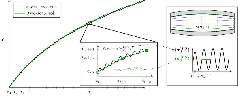
Figure 2: Schematic representation of the two-scale algorithm as described in section 3.1 and summarized in algorithm 1: instead of solving the FSI problem and updating the foam cell concentration $c_{s}$ on the micro time scale ($\delta\tau$, black), we compute an averaged growth function $\overline{\gamma}(\boldsymbol{\sigma}_{f}^{WS})$ over a few periods (heartbeats) of the micro-scale problem (right); this average is used to update $c_{s}$ on the macro scale ($\delta t$, green in the left part).

To be precise, we divide the macro-scale time interval $[0,T_{\text{end}}]$ into $N_{f}$ time steps of size $\delta t$

$$0=t_{0}<t_{1}<...<t_{N_{f}}={T_{\text{end}}},\qquad N_{f}=\frac{T_{\text{end}}}{\delta t}.$$ (13)

As $c_{s}$ varies significantly on the macro scale only, using $c_{s}(t_{m})$ as a fixed value for the growth variable on the micro scale results in a sufficiently good approximation in the time interval $[t_{m},t_{m+1}]$. Then, one cycle of the pulsating blood flow problem (around $1$s) is to be resolved on the micro scale $\delta\tau$

$$0=\tau_{0}<\tau_{1}<....<\tau_{N_{s}}=1s,\qquad N_{s}=\frac{1s}{\delta\tau}.$$ (14)

It has been shown in [29] (for a simplified flow configuration) that this approach leads to a model error ${\cal O}(\epsilon)$ compared to a full resolution of the micro scale, where $\epsilon=\frac{1s}{T_{\text{end}}}$ denotes the ratio between macro- and micro time scale and is in the range of ${\cal O}(10^{-7})$ for a typical cardiovascular plaque growth problem. The relations in eqs. 13 and 14 imply $\delta\tau=\epsilon\delta t$. In the model problems formulated above, the scale separation is induced by the parameter $\alpha={\cal O}(\epsilon)$.

A difficulty lies in solving the periodic micro-scale problem. If accurate initial conditions $\mathbf{w}^{0}:=(\mathbf{v}^{0},\mathbf{u}^{0})$ are available on the micro-scale, a periodic solution can be computed using a time-stepping procedure for one cycle. If the initial conditions are known approximately, convergence to the periodic solution may still be obtained after simulating a few cycles of the micro-scale problem due to the dissipation of the flow problem; see [29, 28]. Numerically, it can be checked after each cycle if the solution is sufficiently close to a periodic state. In this work, we apply a stopping criterion based on the computed averaged growth value:

$$|\overline{\gamma}(\boldsymbol{\sigma}_{f}^{WS,r})-\overline{\gamma}(\boldsymbol{\sigma}_{f}^{WS,r-1})|<\epsilon_{p},$$

where $r=1,2,...$ denotes the iteration index with respect to the number of cycles of the micro-scale problem. The algorithm is summarized as algorithm 1, where we use the abbreviation $\mathbf{w}^{r,s}:=(\mathbf{v}^{r,s},\mathbf{u}^{r,s})$.

Set suitable starting values $\mathbf{w}^{0,0}=(\mathbf{v}^{0,0},\mathbf{u}^{0,0})$ and time-step sizes $\delta t,\delta T$.

for $n=1,2,\dots,N_{f}$ do

1.  

   Micro problem: Set $r\leftarrow 0$

       while $|\overline{\gamma}(\boldsymbol{\sigma}_{f}^{WS,r})-\overline{\gamma}(\boldsymbol{\sigma}_{f}^{WS,r-1})|>\epsilon_{p}$ do

            

• Solve micro-scale problem in eq. 1 in $I_{n}=(t_{n},t_{n}+1s)$

  $$\{\mathbf{w}^{r,0},c_{s}^{n-1}\}\mapsto\{\mathbf{w}^{r,m}\}_{m=1}^{N_{s}}$$

• Compute the averaged growth function

  $$\overline{\gamma}(\boldsymbol{\sigma}_{f}^{WS,r+1})=\frac{1}{N_{s}}\sum_{m=1}^{N_{s}}\gamma(\boldsymbol{\sigma}_{f}^{WS,m}(\mathbf{v}^{r+1,m}),c_{s}^{n-1})$$

  and set $\mathbf{w}^{r+1,0}=\mathbf{w}^{r,N_{s}},\,r\leftarrow r+1$.

 

Macro problem: Update the foam cell concentration $c_{s}^{n}$ by eq. 5 or eq. 11.

Algorithm 1 Two-Scale Algorithm

As starting values $\mathbf{w}^{r,0}=(\mathbf{v}^{r,0},\mathbf{u}^{r,0})$ in step 1. of the algorithm, we use the variables $\mathbf{w}^{r-1,N_{s}}=(\mathbf{v}^{r-1,N_{s}},\mathbf{u}^{r-1,N_{s}})$ from the quasi-periodic state of the previous macro step. It has been observed in [28] that these are usually closer to the starting values of the periodic state than the solution of an averaged stationary problem on the macro scale.

3.2 Numerical example

Before we present the different approaches for parallel time-stepping, let us illustrate the two-scale approach by a first numerical example. Therefore, we use the simple ODE growth model introduced in section 2.2.1, eq. 5. The test configuration introduced here will be used in section 4 as well.

Concerning the geometry we use a two-dimensional channel of length $10$ cm and an initially constant width $\omega(0)$ of $2$ cm as illustrated in fig. 1. The solid parts on the top and bottom corresponding to the arterial wall have an initial thickness of $1$ cm each. Fluid density and viscosity are given by $\rho_{f}=1\,\text{g}/\text{cm}^{3}$ and $\nu_{f}=0.04\,\text{cm}^{2}/\text{s}$, respectively. The growth parameters are set to $\sigma_{0}=30\frac{\text{g\,cm}}{\text{s}^{2}}$ and $\alpha=5\cdot 10^{-7}\frac{1}{\text{s}}$, which yields a realistic time-scale for the arterial plaque growth, see [29]. The solid parameters are $\rho_{s}=1\,\text{g}/\text{cm}^{3}$, $\mu_{s}=10^{4}\,{\text{dyne}/\text{cm}^{2}}$, and $\lambda_{s}=4\cdot 10^{4}\,\text{dyne}/\text{cm}^{2}$. As an inflow boundary condition, we prescribe a pulsating velocity inflow profile on $\Gamma_{f}^{\text{in}}$ given by

$$\mathbf{v}_{f}^{\text{in}}(t,x)=30\begin{pmatrix}\sin(\pi{\frac{t}{\cal P}})^{2}(1-x_{2}^{2})\\ 0\end{pmatrix}\text{cm}/\text{s}.$$ (15)

Here, ${\cal P}=1$ s is the period of a single heartbeat. The symmetry of the configuration can be exploited in order to reduce computational cost by simulating only on the lower half of the computational domain and imposing the symmetry condition $\mathbf{v}_{f}\cdot\vec{n}=0,\,\tau^{T}\boldsymbol{\sigma}_{f}\vec{n}=0$ on the symmetry boundary $\Gamma_{\text{sym}}$, where $\tau$ denotes a tangential vector.

We discretize the FSI problem (1) in time using the backward Euler method. For discretizing the ODE growth model, we use the forward Euler method, which results in

$$c_{s}^{n}=c_{s}^{n-1}+\delta t\,\overline{\gamma}(\boldsymbol{\sigma}_{f}^{WS},c_{s}^{n-1}),\qquad n=1,...,N_{f}.$$ (16)

For spatial discretization, we use biquadratic ($Q_{2}$) equal-order finite elements for all variables and LPS stabilization [11] for the fluid problem. Our mesh, containing both fluid and solid, consists of 160 rectangular grid cells; this corresponds to a total of 3 157 degrees of freedom. The time-step sizes are chosen as $\delta\tau=0.02$ s and $\delta t=0.3$ days; the tolerance for periodicity of the micro-scale problem as $\epsilon_{p}=10^{-3}$. All the computational results have been obtained with the finite element library Gascoigne3d [12]. We use a fully monolithic approach for the FSI problem following Frei, Richter & Wick [30, 48].

In fig. 3, we compare results obtained with the two-scale approach for different macro time-step sizes $\delta t$ with the heuristic averaging approach outlined above; see 2. We see that the pure averaging approach underestimates the growth significantly. Even a very coarse discretization of the macro-scale time interval $\delta t=15$ days in the two-scale approach gives a much better approximation. We note, however, that too coarse time steps might introduce different issues, as the starting values $\mathbf{v}^{0,0}$ and $\mathbf{u}^{0,0}$ might not be good approximations for the periodic state on the micro scale anymore. In combination with a significant mesh deformation for $t\approx 300$ days, this led to divergence of algorithm 1 for an even coarser macro time-step size $\delta t=30$ days. For $\delta t\leq 15$ days, a near-periodic state was reached in 2-3 iterations in each macro-step. A detailed convergence study for a very similar problem has been given in [28].

At the bottom of fig. 3, we show the $L^{2}(\Gamma)$-norm of the wall shear stress over two periods, i.e., 2 seconds, of the micro problem for $\delta t=0.02$s and $\delta T=9$ days. The initial values are taken from the periodic state of the micro problem at the previous macro time-step, i.e., 9 days before. We see that the wall shear stresses converge very quickly to the periodic state. An initial deviation of $6.28\frac{\text{g cm}}{\text{s}^{2}}$ to the periodic reference solution at time $\tau=0.02$ is reduced to $6\cdot 10^{-4}\frac{\text{g cm}}{\text{s}^{2}}$ at time $\tau=1$ within only one period.

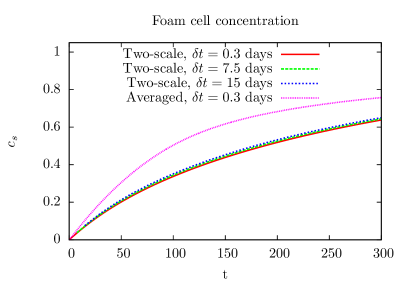
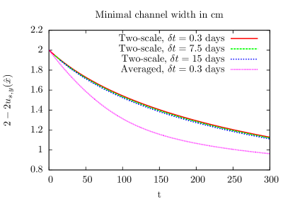
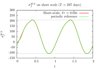
Figure 3: Top: Comparison of a pure averaging approach with the two-scale approaches with different macro-scale time steps $\delta T$. Top left: Concentration $c_{s}$ over time. Top right: Channel width over time. Bottom: Wall shear stress $\boldsymbol{\sigma}_{f}^{WS}$ over two periods of the micro scale at $t=297$ days for $\delta t=9$ days. The initial values are taken from the previous micro problem at $t=288$ days.

4 Parallel time-stepping

The main cost in algorithm 1 lies in the solution of the non-stationary micro problem in step 1.a, which needs to be solved in each time step of the macro problem. Considering a relatively coarse micro-scale discretization of $\delta t=0.02$ s, as used in the previous section, 50 time steps are necessary to compute a single period of the heart beat. The simulation of two or more cycles might be necessary to obtain a near-periodic state in step 1.a of algorithm 1; cf. the discussions in [29, 28]. In a realistic scenario, each time step of the micro problem corresponds to the solution of a complex three-dimensional FSI problem, which makes already the solution of one micro problem very costly.

For this reason, parallelization needs to be exploited in different ways: First, one can make use of spatial parallelization using a scalable solver, for instance, based on domain decomposition or multigrid methods; see, e.g., [35, 33, 39, 58, 9, 19, 36]. Since the focus of this contribution is on parallelization in time, we will not discuss this aspect here. In particular, we expect that even when the speedup due to spatial parallelization saturates, the computing times for the whole plaque growth simulations will remain unfeasible. Therefore, we have to make use of an additional level of parallelization, that is, temporal parallelization of the macro-scale problem. In particular, we will use the parareal algorithm, which we will recap in the next subsection.

In order to motivate the algorithmical developments in this section, we will already present some first numerical results for the ODE growth model in eq. 5 within the section.

4.1 The parareal algorithm

First, the time interval of interest $[0,T_{\text{end}}]$ on the macro scale is divided into $P$ sub-intervals $I_{p}=[T_{p-1},T_{p}]$ of equal size, where

$$0=T_{0}<T_{1}<...<T_{P}=T_{\text{end}}.$$ (17)

In order to define the parareal algorithm, suitable fine and coarse problems need to be introduced. Note again that we will apply the parareal algorithm only on the macro scale as introduced in section 3.1; hence, both the fine and the coarse scale of parareal correspond to the macro scale of the homogenization approach. The fine problem advances the growth variable $c_{s}$ from time $T_{p}$ to $T_{p+1}$ by solving algorithm 1 with a smaller time-step size $\delta t$ (e.g., $0.3$ days) on the corresponding fine time discretization of $[T_{p},T_{p+1}]$:

$$T_{p}=t_{p,0}<t_{p,1}<...<t_{p,n_{p}}=T_{p+1},\qquad n_{p}=\frac{T_{p+1}-T_{p}}{\delta t},\qquad t_{p,q}:=t_{p\cdot n_{p}+q}=t_{p,q-1}+\delta t.$$

The fine propagator on a process $p$ consists of a time-stepping procedure to advance $c_{s}(T_{p})$ to $c_{s}(T_{p+1})$ with the fine time step $\delta t$. We write

$${c_{s}^{\text{fine}}}(T_{p+1})={\cal F}({c_{s}^{\text{fine}}}(T_{p})).$$

The efficiency of the parareal algorithm depends strongly on the computational cost of the coarse propagator. In particular, it needs to be much cheaper than the fine problems since it is defined globally on $[0,T_{\text{end}}]$ and, hence, introduces synchronization. Thus, we use a large time-step $\delta T$ and

$$T_{p}=\bar{T}_{p,0}<...<\bar{T}_{p,N_{p}}=T_{p+1},\qquad N_{p}=\frac{T_{p+1}-T_{p}}{\delta T},\qquad\bar{T}_{p,q}:=\bar{T}_{p\cdot N_{p}+q}=\bar{T}_{p,q-1}+\delta T.$$

For simplicity, we assume that both time-step sizes $\delta t$ and $\delta T$ are uniform throughout $[0,T_{\text{end}}]$. In order to keep the cost of the coarse propagator as low as possible, we will mainly focus on the case that the coarse time steps coincide with the $P$ sub-intervals $I_{p}$ in the numerical results, i.e., $N_{p}=1$, such that the total number of coarse time steps

$$N_{c}:=P\cdot N_{p}$$

is equal to $P$. We denote the coarse propagation from $T_{p}$ to $T_{p+1}$ by

$${c_{s}^{\text{coarse}}}(T_{p+1})={\cal C}({c_{s}^{\text{coarse}}}(T_{p})).$$

We use capital letters $T_{p}$ to denote the coarse discretization of $[0,T_{\text{end}}]$ into $P$ parts and for the time-steps $T_{p,q}$ on the coarse level. By small letters $t_{p,q}$ we denote the finer discretization on each sub-interval; the two discretizations yield the first level (fine problem) and second level (coarse problem) of the parareal algorithm. Of course, it is also possible to employ coarse time steps which differ from the sub-intervals on the fine level, but for the sake of simplicity, we will not discuss this case in this work. In the example given above with $T_{\text{end}}=300$ days, $\delta T$ would be 30 days for $P=N_{c}=10$, while $\delta t$ is 0.3 days. On the micro scale, the times $\tau_{i}$ and time-step size $\delta\tau$ are defined locally in $[t_{i},t_{i}+1s]$; in the example above, we had $\delta\tau=0.02$s. Note that the micro scale influences the parareal algorithm only indirectly due to the temporal homogenization approach.

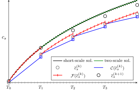
Figure 4: Schematic representation of the parareal algorithm applied to the homogenized (two-scale) problem as shown in fig. 2: micro-scale solution (black), two-scale solution (green), parareal iterates in iteration $k$ (light grey) and $k+1$ (dark grey), fine scale solution (red), and coarse scale solution (blue).

1. Initialization: Compute $\big{\{}(\overline{c}_{s}^{(0)}(T_{p}),\mathbf{w}^{(0)}(T_{p})\big{\}}_{p=1}^{P}$ by means of algorithm 1 with a coarse macro time-step size $\delta T:={(T_{p}-T_{p-1})/N_{p}}$. Set $k\leftarrow 0$

while $|c_{s}^{(k+1),{\text{fine}}}({T_{\text{end}}})-c_{s}^{(k),{\text{fine}}}({T_{\text{end}}})|>\epsilon_{\text{par}}$ do

•  

  Fine problem:

       for $p=1,...,P$ do

• Initialize $c_{s}^{(k+1),{\text{fine}}}(T_{p})=\overline{c}_{s}^{(k)}(T_{p}),\,\mathbf{w}^{(k+1)}(T_{p})=\mathbf{w}^{(k)}(T_{p})$

•        

  Compute $\big{\{}(c_{s}^{(k+1),{\text{fine}}}(t_{p,q}),\mathbf{w}^{(k+1)}(t_{p,q})\big{\}}_{q=1}^{n_{p}}$ by algorithm 1 with fine time-step size

             $\delta t$ and set ${\cal F}(\overline{c}_{s}^{(k)}(T_{p}))=c_{s}^{(k+1),{\text{fine}}}(t_{p,n_{p}})$

 

Coarse problem

       for $p=1,...,P$ do

•        

  Compute ${\cal C}(\overline{c}_{s}^{(k+1)}(T_{p}))$ by solving one time step of algorithm 1 with time-step

size $\delta T={(T_{p}-T_{p-1})/N_{p}}$

       

Parareal update

$$\overline{c}_{s}^{(k+1)}(T_{p+1})={\cal C}(\overline{c}_{s}^{(k+1)}(T_{p}))+{\cal F}(\overline{c}_{s}^{(k)}(T_{p}))-{\cal C}(\overline{c}_{s}^{(k)}(T_{p})).$$

       $k\leftarrow k+1$

Algorithm 2 Parareal algorithm

Then, given an iterate $\overline{c}_{s}^{(k)}$ for some $k\leq 0$, the parareal algorithm computes $\overline{c}_{s}^{k+1}$ by setting

$$\overline{c}_{s}^{(k+1)}(T_{p+1})={\cal C}(\overline{c}_{s}^{(k+1)}(T_{p}))+{\cal F}(\overline{c}_{s}^{(k)}(T_{p}))-{\cal C}(\overline{c}_{s}^{(k)}(T_{p}))\quad\text{ for }\,p=0,...,P-1.$$ (18)

This can be seen as a predictor-corrector scheme, where the coarse predictor ${\cal C}(\overline{c}_{s}^{(k+1)}(T_{p}))$ is corrected by fine-scale contributions that depend only on the previous iterate $\overline{c}_{s}^{(k)}$; thus, the fine problems can be computed fully in parallel. A schematic illustration of the parareal algorithm is given in fig. 4.

Let us analyze the application of eq. 18 to the two-scale problem (algorithm 1) in more detail. The first term in eq. 18 requires the solution of one micro problem and an update of the foam cell concentration (by eq. 5 or eq. 11) in each coarse time step $T_{p}\to T_{p+1}$. Within the fine-scale propagator (second term in eq. 18) $n_{p}=\lceil N_{f}/P\rceil$ time-steps need to be computed per process, where $\lceil g\rceil$ denotes the next-biggest natural number to $g$ ($\widehat{=}$ ceil(g)) and $N_{f}$ is the number of macro time steps; see eq. 13. Each time step requires the solution of one micro problem and an update of the foam cell concentration. The last term in eq. 18 has already been computed in the previous iteration (compare the first term on the right-hand side of the same equation) and thus introduces no additional computational cost. The algorithm is summarized in algorithm 2.

We use the FSI variables $w^{(k)}(T_{p})$ from the previous parareal iteration as initial values in step (II.a)(i). The initial values $\overline{c}_{s}^{(k)}(T_{p})$ in step (II.a)(i) are taken from step (II.b) of the coarse problem. Moreover, to initialize the variables $\{\overline{c}_{s}^{(0)}(T_{p}),\mathbf{w}_{s}^{(0)}(T_{p})\}_{p=1}^{P}$ before the first parareal iteration, we apply the coarse propagator once with a large time-step size $\delta T=(T_{p}-T_{p-1})/N_{p}$.

For the ODE growth model, we use the value of ${c_{s}^{\text{fine}}}$ at the end time $T_{\text{end}}$

$$|c_{s}^{(k+1),{\text{fine}}}(T_{\text{end}})-c_{s}^{(k),{\text{fine}}}(T_{\text{end}})|\leq\epsilon_{\text{par}}.$$ (19)

as the stopping criterion for the parareal algorithm.

4.1.1 Parallelization approaches

Master-slave parallelization

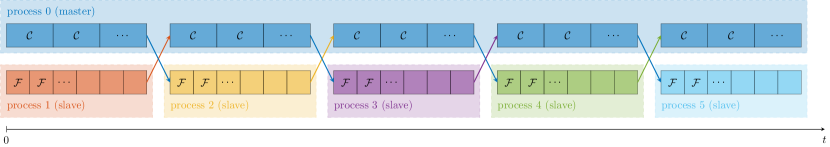
Distributed parallelization

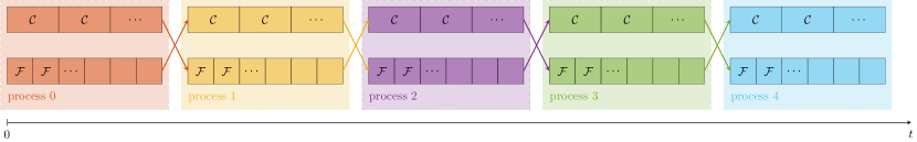
Figure 5: Master-slave and distributed parallelization schemes for the parareal approach. In the master-slave case, the coarse propagation is performed on a separate process (blue) and information is communicated between master and slave. In the distributed case, the coarse propagation and the fine propagation is performed on the same processes. Communication is indicated by an arrow in color of the sender.

As mentioned earlier, in this work, we focus on studying the effectivity and efficiency of our approach by investigating the convergence of the parareal algorithm based on a serial implementation. Since the computational cost of the micro FSI problems is very high, we expect the communication cost to be negligible; cf. section 4.1.2 as well as sections 5.2 and 5.3 for a more detailed discussion of the computational cost for the ODE and the PDE growth model, respectively. Even though our implementation used in the numerical examples below is only serial, we want to briefly discuss two potential parallelization approaches for a parallel implementation of algorithm 2: master-slave parallelization and distributed parallelization; cf. fig. 5 for a sketch of both approaches for our parareal algorithm. Note that, as also indicated by fig. 5, we always assume a one-to-one correspondence of fine problems and processes in this paper.

In the master-slave parallelization approach, the coarse problem is assigned to a single process and the local problems on the fine level are distributed among the remaining processes. Each slave process $p$ has to communicate ${\cal F}(\overline{c}_{s}^{(k)}(T_{p}))$ to the master after computation of the fine problem for the parareal update (step II.a in algorithm 2), and the master process has to communicate $\overline{c}_{s}^{(k+1)}(T_{p})$ back after the parareal update (step II.b in algorithm 2); this corresponds to all-to-one and one-to-all communication patterns.

In the distributed parallelization approach, the parallelization of the coarse problem is different. In particular, time intervals are assigned to the different processes, and each process computes both the fine problem and the part of the coarse problem on those time intervals; for simplicity, we do not discuss the case that the partition of the coarse problem onto the processes is different from the local (fine) problems, which would also be possible. As can be seen in fig. 5, a major benefit of this approach is the different communication pattern: instead of all-to-one and one-to-all communication, each process sends the parareal update $\overline{c}_{s}^{(k+1)}(T_{p})$ to the next process in line. Note that, in terms of the coarse problem, the processes can only perform their computations in serial, whereas the local problems can, again, be computed concurrently.

In some implementations of two-level methods, the coarse problem is assigned to one of the processes dealing with the local problems instead of an additional process; if the memory and computational cost of the coarse problem is negligible, this can be beneficial since all available processes can be employed for the local problems. It can be seen as a mixture of the master-slave and distributed parallelization approaches. In our case, this might not be feasible since the coarse problem is defined on the same spatial mesh as the local problems, leading to significant memory cost. Furthermore, more sophisticated approaches such as task-based scheduling [4] can be employed for the parallelization.

An investigation of the differences in performance of the different approaches can only be performed using an actual parallel implementation. This is out of the scope of this paper, and therefore, we will leave it to future work.

4.1.2 Computational costs

Even in the simplified two-dimensional configuration considered in this work, it suffices to count the number of micro problems to be solved to estimate the computational cost of corresponding parallel computations and to compare different algorithms. Remember that, in each micro problem, $r_{p}\cdot\frac{1}{\delta t}$ FSI systems need to be solved, where $r_{p}$ is the number of cycles required to reach a near-periodic state. In the example considered above, these were at least $2\cdot\frac{1}{0.02}=100$ costly FSI problems. Hence, our discussion in the following sections will be based on the assumption that the computational cost for all other steps of the parareal algorithm as well as the communication between the processes can be neglected. This is particularly obvious for the ODE growth model in eq. 5. For the PDE growth model in eq. 11, we will discuss the computational and communication cost in more detail in sections 5.2 and 5.3.

To analyze the computational cost of algorithm 2 under this assumption, let us denote the total number of iterations of the parareal algorithm by $k_{\text{par}}$. As discussed in sections 4.1 and 4.1.1, we assume that the number of coarse time steps is the same as the number of fine problems and processes, respectively. Therefore, we need to solve $N_{c}$ micro problems in step I, $k_{\text{par}}\cdot\lceil N_{f}/P\rceil$ micro problems on each of the $P$ processes in step II.a (ii), and $k_{\text{par}}\cdot{N_{c}}$ micro problems within the coarse propagation in step II.b (i). This corresponds to the solution of

$$\underbrace{k_{\text{par}}\cdot\lceil N_{f}/P\rceil}_{\text{fine level ($P$ parallel processes)}}+\underbrace{(k_{\text{par}}+1)\cdot{N_{c}}}_{\text{coarse level (1 serial process)}}$$ (20)

serial micro problems; this is the case for both parallelization approaches discussed in section 4.1.1. If the coarse time step $\delta T$ is chosen independently of $T$, $N_{c}$ is fixed and the computational cost tends to saturate for large $P$ (at least if we assume that the number of required parareal iterations $k_{\text{par}}$ is independent of $P$). The cheapest possible coarse propagator, on the other hand, is to use one coarse time step per coarse propagation, i.e., $N_{p}=1$ and $N_{c}=P$. In this case the computational time increases for large $P$, if we assume that the number of parareal iterations $k_{\text{par}}$ is independent of $P$. The minimum computational time is attained for $P\approx\sqrt{N_{f}}$.

As a serial implementation requires the solution of $N_{f}$ micro problems, the speed-up of the proposed parareal algorithm is given by

$$\text{speedup}(P)=\frac{N_{f}}{k_{\text{par}}\cdot\lceil N_{f}/P\rceil+(k_{\text{par}}+1)\cdot{N_{c}}}\approx\frac{1}{\frac{k_{\text{par}}}{P}+(k_{\text{par}}+1)\frac{N_{c}}{N_{f}}},$$ (21)

if we assume a perfect load balancing on the fine processes. This is a special case of the standard analysis for the speed-up of the parareal algorithm; see, e.g., [52].

The aim of this work is to show potential for the parareal algorithm as a parallel time-stepping method for plaque growth simulations. A final assessment of the parallelization capabilities can, of course, only be made based on computing times of an actual parallel implementation. We will leave this to future work.

4.1.3 Convergence theory

Let us briefly recap the standard convergence theory for the parareal algorithm; see, e.g., [32]. For this purpose, let us consider the simpler ODE model

$$\partial_{t}c_{s}=\gamma(c_{s}),\qquad c_{s}(0)=0.$$ (22)

and its discretization by the explicit Euler method

$$c_{s}^{n}=c_{s}^{n-1}+\delta T\,\gamma(c_{s}^{n-1}),\qquad c_{s}^{0}=0.$$ (23)

We assume that the function $\gamma$ and its derivative are Lipschitz continuous in $c_{s}$, i.e., we assume

$$|\gamma(c_{s}^{1})-\gamma(c_{s}^{2})|\leq L|c_{s}^{1}-c_{s}^{2}|,\quad\big{|}\frac{d}{dt}\gamma(c_{s}^{1})-\frac{d}{dt}\gamma(c_{s}^{2})\big{|}\leq L|c_{s}^{1}-c_{s}^{2}|\quad\text{for all }c_{s}^{1},c_{s}^{2}\in\mathbb{R}$$ (24)

for some $L>0$. As in [32], we also assume for simplicity that the fine-scale propagator advances the ODE exactly, i.e.,

$$c_{s}(T_{n})={\cal F}(c_{s}(T_{n-1}))=c_{s}(T_{n-1})+\int_{T_{n-1}}^{T_{n}}\gamma(c_{s}(s))\,\text{d}s.$$ (25)

This is motivated by the fact that the time discretization error in the fine propagator is typically small compared to the coarse propagator. The following convergence result is shown by Gander & Hairer in [32]:

Lemma 1.

Let $c_{s}^{*}\in C^{1}(0,T_{\text{end}})$ be the exact solution of eq. 22, and let $\{\overline{c}_{s}^{(k)}(T_{n})\}_{n=1}^{P}$ be the $k$-th iterate of the parareal algorithm in eq. 18 using the forward Euler method in eq. 23 as the time discretization. Under the assumptions made above, it holds for the error $e_{n}^{(k)}=|\overline{c}_{s}^{(k)}(T_{n})-c_{s}^{*}(T_{n})|$ and $k\in\mathbb{N}_{0},n\in\{1,\ldots,P\}$ that

$$e_{n}^{(k)} \leq\left(cT_{n}\right)^{k+1}\beta^{n-k-1}\delta T^{k+1}\max_{t\in[0,T_{\text{end}}]}|\partial_{t}c_{s}^{*}(t)|.$$ (26)

with a constant $c>0$ and $\beta=1+L\delta T$.

Remark 1.

The assumptions in eq. 24 cannot be easily verified for the ODE model in eq. 5, as the fluid forces and $\bar{\gamma}(\sigma_{f}^{WS})$ depend in a highly nonlinear way on $c_{s}$. In the numerical examples given below, we will, however, observe that the convergence behavior is similar to the one shown in lemma 1.

4.1.4 Numerical results

We use, again, the simple example described in section 3.2 with the ODE growth model in eq. 5 and set $\epsilon_{\text{par}}=10^{-3}$. Results for $P=N_{c}=10$ and $\delta t=0.3$ days are shown in fig. 6, where the first 3 iterates are compared against a reference solution $(c_{s}^{*},\mathbf{u}_{s}^{*},\mathbf{v}_{f}^{*})$, which was computed by a standard serial time-stepping scheme, as in section 3.2. We observe fast convergence towards the reference curve in all three quantities of interest. The stopping criterion in eq. 19 was satisfied after 4 iterations of the parareal algorithm.

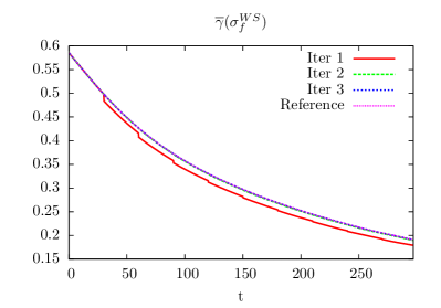
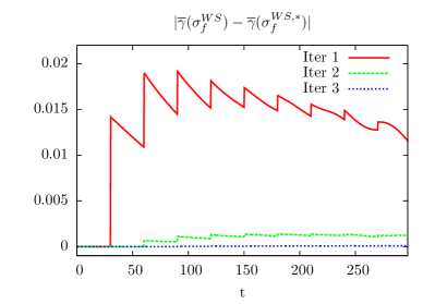
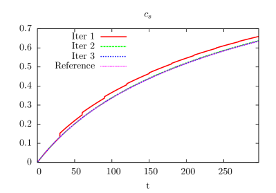
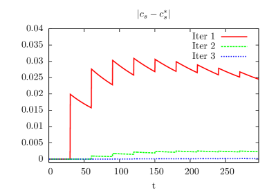
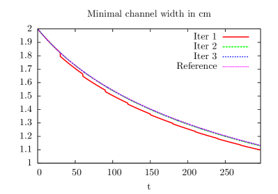
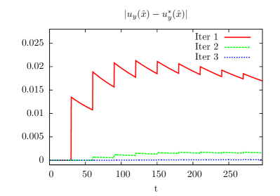
Figure 6: Behavior of the first three iterates of the parareal algorithm in the first numerical example (ODE growth) for $P=10$. A description of the problem is given in section 4.1.4, numerical values in table 1. The iterates converge very quickly towards the reference solution. Top: Growth function and error w.r.t the reference solution $\boldsymbol{\sigma}_{f}^{WS}(\mathbf{v}_{f}^{*})$ over time $t$. Center: $c_{s}^{(k),\text{fine}}$ and error w.r.t the reference solution $c_{s}^{*}$ over time. Bottom: Channel width over time and error $|\mathbf{u}_{s,y}(\hat{x})-\mathbf{u}_{s,y}^{*}(\hat{x})|$ w.r.t. the vertical component of the reference solution $\mathbf{u}_{s}^{*}$ at the narrowest point $\hat{x}$ over time .

k	$P=10$	$P=20$	$P=30$	$P=40$	$P=50$	ref. (serial)
1	$2.21\cdot 10^{-2}$	$1.19\cdot 10^{-2}$	$8.12\cdot 10^{-3}$	$5.83\cdot 10^{-3}$	$5.46\cdot 10^{-3}$	0
2	$2.24\cdot 10^{-3}$	$5.63\cdot 10^{-4}$	$2.62\cdot 10^{-4}$	$1.37\cdot 10^{-4}$	$8.61\cdot 10^{-5}$	-
3	$1.42\cdot 10^{-4}$	$2.02\cdot 10^{-5}$	$6.53\cdot 10^{-6}$	$2.32\cdot 10^{-6}$	$8.30\cdot 10^{-7}$	-
4	$5.76\cdot 10^{-6}$	-	-	-	-	-
# mp	450	230	222	235	260	1 000
speedup	2.2	4.3	4.5	4.3	3.8	1.0
efficiency	22 %	22 %	15 %	11 %	8 %	100 %

Table 1: Errors $|c_{s}^{(k),{\text{fine}}}(T_{\text{end}})-c_{s}^{*}(T_{\text{end}})|$ for $P=10,\ldots,50$ for the parareal algorithm (algorithm 2) in the first numerical example (ODE growth). For comparison, the reference value $c_{s}^{*}(T_{\text{end}})=0.63831273...$ resulting from a serial time-stepping with the same fine-scale time-step size $\delta t$ is taken. The time measure in terms of the number of serial micro problems (# mp) as well as speedup and efficiency compared to the reference computation (right column) are shown; the stopping criterion $|c_{s}^{(k+1),{\text{fine}}}(T_{\text{end}})-c_{s}^{(k),{\text{fine}}}(T_{\text{end}})|<\epsilon_{\text{par}}=10^{-3}$ is used; best numbers marked in bold face.

In table 1, we show the deviations in the foam cell concentration $|c_{s}^{(k),{\text{fine}}}(T_{\text{end}})-c_{s}^{*}(T_{\text{end}})|$ at final time $T_{\text{end}}$ after each iteration of the parareal algorithm for $P=N_{c}=10,20,30,40$ and $50$ processes. We observe that the number of iterations $k_{\text{par}}$ decreases from four to three for $P\geq 20$. This is due to the fact that the coarse problem is solved with the smaller time-step size $\delta T=\lceil\frac{T_{\text{end}}}{P}\rceil$, which makes the coarse problem more expensive but also more accurate. In particular, we obtain a better approximation for the coarse values $\overline{c}_{s}^{(k)}(T_{p})$ that are used as initial values in the fine problems in the next iterate. We can also observe that, for fixed $P$, the error decreases at least by a factor $\frac{1}{P}$ in each parareal iteration. This is in agreement with lemma 1, which predicts (for a simpler model problem) a reduction factor $c\cdot\delta T=c\cdot\lceil\frac{T_{\text{end}}}{P}\rceil$ for some constant $c>0$, compared to the previous iterate.

Since the number of parareal iterations $k_{\text{par}}$ is constant for all cases with $P\geq 20$, we get the lowest computational cost for $P=30$, which is close to $\sqrt{N_{f}}\approx 31.6$; cf. the discussion in section 4.1.2. For $P=30$, $3\cdot 34=102$ micro problems need to solved on each process (step II.a) and $4\cdot 30=120$ micro problems within the coarse propagators (steps I and II.b), i.e., $222$ micro problems in total. Compared to a serial time-stepping scheme with the same fine-scale time-step size, which requires the solution of $N_{f}=1\,000$ serial micro problems, this corresponds to a speed-up of $\frac{1\,000}{222}\approx 4.5$; see also eq. 21. As is usual for two-level methods, for larger numbers of processes ($P$), the cost of the coarse problems gets dominant. For $P=40$, we solve, for example, $3\cdot 25=75$ micro problems in the fine propagator compared to $4\cdot 40=160$ micro problems for the coarse propagator; this results in a total of $235$ micro problems and a speedup of $4.3$.

k	$P=10$	$P=20$	$P=30$	$P=40$	$P=50$	ref. (serial)
1	$2.59\cdot 10^{-3}$	$5.97\cdot 10^{-4}$	$3.29\cdot 10^{-4}$	$1.42\cdot 10^{-4}$	$8.95\cdot 10^{-5}$	0
2	$2.81\cdot 10^{-3}$	$2.04\cdot 10^{-5}$	$6.59\cdot 10^{-6}$	$2.36\cdot 10^{-6}$	$8.43\cdot 10^{-7}$	-
3	$6.37\cdot 10^{-6}$	-	-	-	-	-
4	$1.73\cdot 10^{-7}$	-	-	-	-	-
# mp	450	160	158	170	190	1 000
speedup	2.2	6.25	6.3	5.9	5.3	1.0
efficiency	22 %	31 %	21 %	15 %	11 %	100 %

Table 2: Errors $|\overline{c}_{s}^{(k)}(T_{\text{end}})-c_{s}^{*}(T_{\text{end}})|$ for $P=10,\ldots,50$ for the parareal algorithm (algorithm 2) in the first numerical example (ODE growth). The time measure in terms of the number of serial micro problems (# mp) as well as speedup and efficiency compared to the reference computation (right column) are shown; the stopping criterion $|\overline{c}_{s}^{(k+1)}(T_{\text{end}})-\overline{c}_{s}^{(k)}(T_{\text{end}})|<\epsilon_{\text{par}}=10^{-3}$ is used; best numbers marked in bold face.

In order to relate the speed-up to the computational resources used, we define the computational efficiency by the ratio ${\displaystyle\frac{\text{speedup}}{P}}$ as a second measure to quantify the results. By definition, the serial computation always has the best efficiency, as it converges within one sweep through all time steps. Even if the parareal algorithm would also converge within one iteration, the parallel computations come with additional costs since they require the solution of the coarse problem.

In fact, using the serial computation as a reference in the comparison in table 1, the efficiency is best ($22\,\%$) for $P=10$ or $P=20$; it deteriorates for larger numbers of processes due to the increasing cost of the coarse problems. The low efficiency is a typical observation for parallel time integration methods, such as the parareal method and can be explained as follows: For $P=10$, for instance, 4 parareal iterations are required and each iteration requires the solution of all 1 000 micro problems on the fine scale on the full time interval $[0,T_{\text{end}}]$. Hence, a total of 4 000 micro problems has to be solved. Assuming that the time to solve a micro problem is approximately constant, we can not expect efficiencies above 25%. Due to the additional cost of the coarse propagator, the efficiency is reduced to 22%. However, since we can always compute 10 micro problems on the fine scale at the same time, we can still obtain a speedup of 2.2.

To increase the efficiency, we could take the value $\overline{c}_{s}^{(k)}(T_{\text{end}})$ computed in eq. 18 instead of $c_{s}^{(k),{\text{fine}}}(T_{\text{end}})$ in the stopping criterion

$$|\overline{c}_{s}^{(k+1)}(T_{\text{end}})-\overline{c}_{s}^{(k)}(T_{\text{end}})|<\epsilon_{\text{par}}.$$ (27)

In particular, at the end time $T_{\text{end}}$ we expect that this has a higher accuracy compared to the fine-scale variable $c_{s}^{(k),{\text{fine}}}(T_{\text{end}})$. However, the values $\overline{c}_{s}^{(k+1)}(t_{i})$ are only available at the coarse grid points $t_{i}\in\{T_{p}\}_{p=1}^{P}$. If one is interested in foam cell concentrations at intermediate time steps, a stopping criterion based on $c_{s}^{(k),{\text{fine}}}(t_{i})$ needs to be used, as in eq. 19.

The errors concerning $\overline{c}_{s}^{(k)}(T)$ and the number of micro problems to be solved using the stopping criterion eq. 27 are given in table 2. We observe that for $P\geq 20$ this stopping criterion was satisfied already after $k_{\text{par}}=2$ iterations. For $P=30$ we get again the lowest computational cost with a speed-up of around $6.33$ compared to a serial computation. Furthermore, the best efficiency is obtained here with $P=20$, which is due to the lower iteration count compared to the case $P=10$.

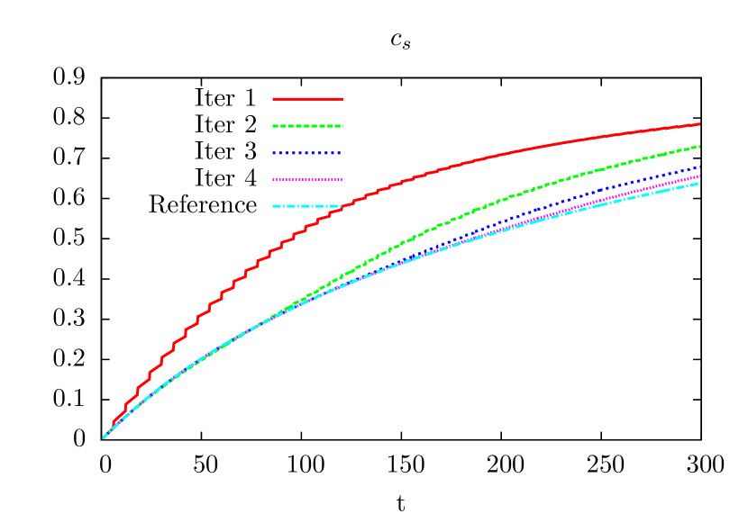
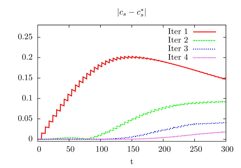
k	$P=30$	$P=50$	ref. (serial)
1	$1.66\cdot 10^{-1}$	$1.42\cdot 10^{-1}$	0
2	$9.34\cdot 10^{-2}$	$9.34\cdot 10^{-2}$	-
3	$4.86\cdot 10^{-2}$	$4.06\cdot 10^{-2}$	-
4	$1.84\cdot 10^{-2}$	$1.76\cdot 10^{-2}$	-
5	$5.41\cdot 10^{-3}$	$5.71\cdot 10^{-3}$	-
6	$1.28\cdot 10^{-3}$	$1.47\cdot 10^{-3}$	-
7	$2.47\cdot 10^{-4}$	$3.14\cdot 10^{-4}$	-
8	$4.79\cdot 10^{-5}$	$6.48\cdot 10^{-5}$	-
# mp	272	160	1 000
speedup	3.7	6.3	1.0
eff.	12 %	13 %	100 %

Figure 7: Behavior of the iterates of the parareal algorithm, when the stationary FSI problem (2) is used in Step (I) and (II.b)(i) of algorithm 2. A description of the computation is given in section 4.2. Convergence to the reference solution is much slower compared to standard parareal (see fig. 6). Top: Evolution of $c_{s}^{(k),{\text{fine}}}(t)$ and error $|c_{s}^{(k),\text{fine}}(t)-c_{s}^{*}(t)|$ of the foam cell concentration over time $t$ for $P=50$ and $k=1,2,3,4$. Right: Errors $|c_{s}^{(k),{\text{fine}}}(T_{\text{end}})-c_{s}^{*}(T_{\text{end}})|$ after each iteration for $P=30$ and $P=50$; total number of micro problems (# mp) solved in parallel as well as speedup and efficiency compared to the reference computation (right column); best numbers marked in bold face.

4.2 Variants with cheaper coarse-scale computations

In the parareal algorithm introduced above, a further improvement of the computational cost is not possible for $P\gtrsim\sqrt{N_{f}}$ processes in the case $P=N_{c}$ due to the (increasing) cost of the coarse-scale propagators. In fact, these get dominant compared to the fine-scale contributions for $P\gtrsim\sqrt{N_{f}}$. In this section, we will discuss approximate coarse-scale propagators, where no additional computations of micro problems are needed; hence, they are computationally cheaper.

4.2.1 Heuristic averaging of the FSI problems

As a first variant, we use the heuristic averaging approach mentioned in the beginning of section 3.1 for the coarse-scale propagation in steps (I) and (II.b)(i) of algorithm 2. The solution of the stationary FSI problem in 2 is much cheaper compared to $\geq 100$ time steps of a non-stationary FSI problem (approx. by a factor 100), and thus, its computational cost is neglected in the following discussion. Hence, the computational cost is reduced from $k_{\text{par}}\cdot\lceil N_{f}/P\rceil+(k_{\text{par}}+1)\cdot P$ to $k_{\text{par}}\cdot\lceil N_{f}/P\rceil$ micro problems. In fig. 7, we illustrate the error in the foam cell concentration for $P=50$ (left), and give the error $|c_{s}^{(k),{\text{fine}}}(T_{\text{end}})-c_{s}^{*}(T_{\text{end}})|$ in each iteration $k$ for $P=30$ and $P=50$ (right). We observe a much slower convergence compared to the standard parareal algorithm used above. This could already be expected from the results in fig. 3, where we saw that the heuristic averaging is not a good approximation. Using the stationary problem for the coarse propagator, $8$ parareal iterations are necessary until the stopping criterion is satisfied for $P=30$ and $P=50$ compared to $3$ iterations in the standard parareal algorithm.

In terms of the computating time, $8\cdot 34=272$ and $8\cdot 20=160$ micro problems are necessary for the cases $P=30$ and $P=50$, respectively. While for $P=30$ this is worse compared to the standard parareal algorithm, this is an improvement of $67\%$ for $P=50$; cf. table 1. As for the standard parareal algorithm, convergence is obtained faster if we consider the stopping criterion in eq. 27 based on the parareal iterates $\overline{c}_{s}^{(k)}(T_{\text{end}})$; however, $7$ iterations are still needed. The resulting computational cost is $7\cdot 34=238$ micro problems for $P=30$ and $7\cdot 20=140$ micro problems for $P=50$. Compared to 158 micro problems for $P=30$ and 190 micro problems for $P=50$ in the standard parareal algorithm (cf. table 2), we see only a small but no significant improvement. We will thus consider another, more promising approach to compute the required growth values $\gamma(\boldsymbol{\sigma}_{f}^{WS})$ for the coarse propagator in the following subsection.

Remark 2.

As mentioned before, parallelization in space is generally more efficient than parallelization in time. Hence, complex three-dimensional FSI simulations already have a significant potential for parallelization. Additionally using temporal parallelization with large values of $P$, such as $P>50$, may only be reasonable on very large supercomputers.

4.2.2 Re-usage of computed growth values

As a second approach we will consider the re-use of growth values $\overline{\gamma}(\boldsymbol{\sigma}_{f}^{WS}(t_{p,i}))$ computed in the fine-scale propagator on the coarse scale. Therefore, we store all values $\overline{\gamma}_{p\cdot n_{p}+i}:=\overline{\gamma}(\boldsymbol{\sigma}_{f}^{WS}(t_{p,i}))$ computed on the fine scale on all processes $p=1,...,P$ for all time-steps $i=1,...,n_{p}$; see step 1.b of algorithm 1. These can be used in the coarse propagator (step II.b) in the same parareal iteration instead of computing new growth values there.

We introduce the following notations for the coarse resp. fine propagators that start from $c_{s,n-1}$ using certain growth values $\gamma(T_{n-1})$ (that might now differ from $\overline{\gamma}(\sigma_{f}^{\text{WS}}(c_{s,n-1}))$):

$$c_{s,n}^{\text{coarse}}={\cal C}(I_{n},c_{s,n-1},\gamma(T_{n-1})),\quad c_{s,n}^{\text{fine}}={\cal F}(I_{n},c_{s,n-1},\gamma(T_{n-1})),$$

where $I_{n}=[t_{n-1},t_{n}]$. After an initialization step, the modified parareal iteration is defined by the following formula for $n=1,...,P$ and $k\geq 1$:

$$\overline{c}_{s,n}^{(k)}={\cal C}(I_{n},\overline{c}_{s,{n-1}}^{(k)},\bar{\gamma}(c_{s,n-1}^{(k),\text{fine}}))+{\cal F}(I_{n},\overline{c}_{s,n-1}^{(k-1)},\bar{\gamma}(\overline{c}_{s,n-1}^{(k-1)}))-{\cal C}(I_{n},\overline{c}_{s,n-1}^{(k-1)},\bar{\gamma}(c_{s,n-1}^{(k-1),\text{fine}})),$$ (28)

where

$$c_{s,n-1}^{(k),\text{fine}}:={\cal F}(I_{n-1},\overline{c}_{s,n-2}^{(k-1)},\bar{\gamma}(\overline{c}_{s,n-2}^{(k-1)})),$$ (29)

and $c_{s,n}^{(0),\text{fine}}=\overline{c}_{s,n}^{(0)}$. Moreover, we set $c_{s,0}^{(k),\text{fine}}=\overline{c}_{s,0}^{(k)}=0$ for all $k$.

As no new micro problems need to be solved and approximations of the growth values $\overline{\gamma}_{j}$ are available for all fine time steps $j=1,...,N_{f}$, the coarse propagator can now even use the fine-scale time-step $\delta t$. The only additional cost is to advance the foam cell concentration by eq. 5 resp. eq. 18 on the coarse level. This cost is clearly negligible for the ODE growth model in eq. 5. The additional cost in case of the PDE model eq. 18 will be discussed in section 5. The resulting algorithm is given as algorithm 3.

1. Initialization: Compute $\big{\{}(\overline{c}_{s}^{(0)}(T_{p}),\overline{\mathbf{w}}^{(0)}(T_{p})\big{\}}_{p=1}^{P}$ by means of algorithm 1 with a coarse macro time-step size $\delta T=T_{p+1}-T_{p}$ on the master process. Set $k\leftarrow 0$

while $|c_{s}^{(k+1),{\text{fine}}}({T_{\text{end}}})-c_{s}^{(k),{\text{fine}}}({T_{\text{end}}})|>\epsilon_{\text{par}}$ do

•  

  Fine problem:

       for $p=1,...,P$ do

• Initialize $c_{s}^{(k+1),{\text{fine}}}(T_{p})=\overline{c}_{s}^{(k)}(T_{p}),\,\mathbf{w}^{(k+1)}(T_{p})=\mathbf{w}^{(k)}(t_{p-1,N_{p}}))$

• Compute $\big{\{}(c_{s}^{(k+1),{\text{fine}}}(t_{p,q}),\mathbf{w}^{(k+1)}(t_{p,q})\big{\}}_{q=1}^{n_{p}}$ by algorithm 1 with fine time step $\delta t$

•        

  Store the resulting growth functions $\overline{\gamma}_{p\cdot n_{p}+q}:=\overline{\gamma}(\boldsymbol{\sigma}_{f}^{WS})(t_{p,q})$ at all fine points

            $t_{p,q},\,q=1,...,n_{p}$ as well as $\mathbf{w}(t_{p,n_{p}})$ at the last time-step.

Coarse problem:

•  

  for $j=1,...,N_{f}$ do

                              Compute $\overline{c}_{s}^{(k+1)}(t_{j})$ by advancing the ODE eq. 5 resp.  solving the PDE

                               in eq. 11 using the growth values $\overline{\gamma}_{j}$ computed in (II.a).

      

Algorithm 3 Parallel Time-Stepping with Re-Usage of Growth Values

The growth values employed for the re-usage are available for all fine-scale time steps, and hence, we are able to perform the coarse propagation efficiently on the fine scale; cf. the discussion on the computational cost later in this section as well as for the PDE growth model in section 5.3. Nonetheless, the expected accuracy of the re-usage approach is still lower compared to the standard parareal algorithm. This is because the growth values on the fine scale have been computed using $c_{s,n-1}^{(k),\text{fine}}$, which depends on the previous iterate $\overline{c}_{s,n-2}^{(k-1)}$ (see eq. 29), whereas the coarse propagator in the standard parareal algorithm already uses the more accurate $\overline{c}_{s,n-1}^{(k)}$ from the current iteration.

Computational costs

Only the coarse step in the initialization (I) has to be carried out without re-usage and comes with a computational cost of $N_{c}$ micro problems. On the other hand, step (II.b) does not require the solution of any micro problems. In terms of micro problems to be solved, the computational cost of step (II.a) is the same as in the standard parareal algorithm (algorithm 2). Altogether, the number of micro problems to be solved in $k_{\text{par}}$ iterations of algorithm 3 is

$$k_{\text{par}}\cdot\lceil N_{f}/P\rceil+{N_{c}}.$$

Again, we obtain a saturation of the cost for large $P$, but the cost for large $P$ is by a factor $k_{\text{par}}$ smaller. Moreover, for $N_{c}=P$, the choice $P\approx\sqrt{k_{\text{par}}N_{f}}$ would be optimal if the number of iterations $k_{\text{par}}$ was independent of the number of processes $P$.

The speed-up compared to a serial computation is given by

$$\text{speedup}(P)=\frac{N_{f}}{k_{\text{par}}\cdot\lceil N_{f}/P\rceil+N_{c}}\approx\frac{1}{\frac{k_{\text{par}}}{P}+\frac{N_{c}}{N_{f}}},$$ (30)

assuming, again, a perfect load balancing of the micro problems.

The communication cost of the approach strongly depends on the employed parallelization scheme; cf. section 4.1.1. In the distributed parallelization approach, the growth values $\overline{\gamma}(\boldsymbol{\sigma}_{f}^{WS}(t_{p,i}))$, which are needed in the coarse propagator, do not have to be communicated. This is because the same intervals in fine and coarse problems are computed on the processes. In the master-slave approach, however, the values have to be communicated from each slave process to the master. Using the ODE growth model, these are $N_{f}$ scalar values in total (in our example $N_{f}=1\,000$). Even for the master-slave communication scheme, it is thus reasonable to assume that the computational cost of communication is still negligible compared to the solutions of the micro problems. In the case of a PDE growth model, the additional cost for communication will be discussed in section 5.

Theoretical convergence analysis

We extend the convergence results discussed in section 4.1.3 for the model problem in eq. 22 for the re-usage algorithm in eq. 28 under the assumptions made in section 4.1.3.

The following result is a direct consequence of lemma 3, which is shown in the appendix.

Theorem 1.

Let $c_{s}^{*}\in C^{1}(0,T_{\text{end}})$ be the exact solution of eq. 22 and let $\{\overline{c}_{s}^{(k)}(T_{n})\}_{n=1}^{P}$ be the $k$-th iterate of the re-usage algorithm in eq. 28 using the forward Euler method in eq. 23. Under the assumptions made in section 4.1.3, it holds for the error $e_{n}^{(k)}=|\overline{c}_{s}^{(k)}(T_{n})-c_{s}^{*}(T_{n})|$ and $k\in\mathbb{N}_{0},n\in\{1,\ldots,P\}$ that

$$e_{n}^{(k)} \leq L\delta T\max\left\{1,T_{n-\frac{k}{2}}\right\}^{k}\frac{c^{k}\beta^{n-k}}{\lceil\nicefrac{{k}}{{2}}\rceil!}\max_{t\in[0,T_{\text{end}}]}|\partial_{t}c_{s}^{*}(t)|.$$ (31)

with a constant $c>0$ (see lemma 3) and $\beta=1+L\delta T$. This implies $e_{n}^{(k)}\to 0$ for $k\to\infty$.

The convergence $e_{n}^{(k)}\to 0$ for $k\to\infty$ follows due to the faculty ${\lceil\nicefrac{{k}}{{2}}\rceil!}$ in the denominator. Compared to lemma 1, the estimated convergence in $k$ is much slower. However, we will observe in the numerical examples below that a good accuracy might still be reached within few iterations.

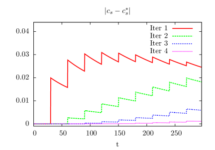
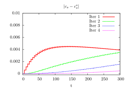
Figure 8: Error in the concentration $|c_{s}^{(k),\text{fine}}(t)-c_{s}^{*}(t)|$ over time $t$ in the first 3 iterates of the parareal algorithm with re-usage of growth values (algorithm 3) for $P=10$ (left) and $P=60$ (right) and the first numerical example (ODE growth model).

k	$P=10$	$P=20$	$P=30$	$P=40$	$P=50$	$P=60$	$P=70$	ref.
1	$2.56\cdot 10^{-2}$	$1.10\cdot 10^{-2}$	$7.48\cdot 10^{-3}$	$5.46\cdot 10^{-3}$	$4.23\cdot 10^{-3}$	$3.63\cdot 10^{-3}$	$3.12\cdot 10^{-3}$	0
2	$7.78\cdot 10^{-3}$	$4.48\cdot 10^{-3}$	$3.16\cdot 10^{-3}$	$2.36\cdot 10^{-3}$	$1.99\cdot 10^{-3}$	$1.61\cdot 10^{-3}$	$1.41\cdot 10^{-3}$	-
3	$1.73\cdot 10^{-3}$	$1.20\cdot 10^{-3}$	$9.02\cdot 10^{-4}$	$6.92\cdot 10^{-4}$	$6.34\cdot 10^{-4}$	$5.14\cdot 10^{-4}$	$4.32\cdot 10^{-4}$	-
4	$2.32\cdot 10^{-4}$	$2.28\cdot 10^{-4}$	$1.87\cdot 10^{-4}$	$1.31\cdot 10^{-4}$	$1.26\cdot 10^{-4}$	$1.10\cdot 10^{-4}$	$9.98\cdot 10^{-5}$	-
5	$2.19\cdot 10^{-5}$	$4.71\cdot 10^{-5}$	$3.05\cdot 10^{-5}$	-	-	-	-	-
# mp	510	270	200	140	130	128	130	1 000
speedup	2.0	3.7	5.0	7.1	7.7	7.8	7.7	1.0
eff.	20 %	19 %	17 %	18 %	15 %	13 %	11 %	100 %

Table 3: Errors $|c_{s}^{(k),{\text{fine}}}(T_{\text{end}})-c_{s}^{*}(T_{\text{end}})|$ for $P=10,\ldots,70$ for the parareal algorithm 3 (re-use of growth values) and the first numerical example (ODE growth model). Value $c_{s}^{*}(T_{\text{end}})$ of a serial reference computation for comparison. The time measure in terms of the number of micro problems (# mp) as well as speedup and efficiency compared to the reference computation (right column) are shown; the stopping criterion $|c_{s}^{(k+1),{\text{fine}}}(T_{\text{end}})-c_{s}^{(k),{\text{fine}}}(T_{\text{end}})|<\epsilon_{\text{par}}=10^{-3}$ is used; best numbers marked in bold face.

Numerical results

In fig. 8, the evolution of the error in the concentration variable $c_{s}^{(k)}$ is plotted over time for $P=N_{c}=10$ and $P=N_{c}=60$. We observe convergence to the reference values $c_{s}^{*}$ in both cases. Compared to the results in fig. 6 for the classical parareal algorithm (algorithm 2), the convergence is significantly slower. Nevertheless, the stopping criterion is already fulfilled after 4-5 iterations (see table 3), which is only 1-2 iterations more than in the standard parareal algorithm (see table 1).

While we had observed reduction factors in the order of $\delta T=\lceil\frac{T_{\text{end}}}{P}\rceil$ between two consecutive parareal iterations for the standard parareal algorithm in table 1, the reduction factors are slightly worse in table 3. They are, however, in all cases (besides the last value for $P=20$) bounded above by $\frac{1}{k}$, where $k$ is the parareal iterate. This indicates a convergence of order ${\cal O}(\frac{1}{k!})$, which is related to the factor ${\cal O}(\frac{1}{\lceil\frac{k}{2}\rceil!})$ in eq. 31 in theorem 1. Moreover, the absolute values of the error in each parareal iteration are significantly smaller for $P=60$ compared to the case of $P=10$ (Note the different scaling in the vertical axis).

In table 3, we compare the number of micro problems needed for $P=N_{c}=10$ to $70$. The optimal number of processes is $P=\sqrt{k_{\text{par}}N_{f}}\approx 63.25$, which is twice as many processes compared to the parareal algorithm in the previous section. The minimal cost in table 3 is 128 micro problems for $P=60$, compared to 222 for standard parareal. Compared to a serial time-stepping scheme, we obtain a maximum estimated speed-up of 7.8. Moreover, the efficiency is also significantly improved for larger numbers of processes compared to the standard approach; cf. tables 1 and 3.

5 Plaque growth problem with a distributed foam cell concentration

We consider the PDE growth model introduced in section 2.2.2, where the concentration of foam cells $\hat{c}_{s}=\hat{c}_{s}(\hat{x},t)$ is now governed by the non-stationary reaction-diffusion problem in eq. 11. For time discretization, we use a linearized variant of the backward Euler scheme. Starting from $c_{s,0}=0$, the standard backward Euler scheme writes for $l=1,...,N_{f}$:
Find ${c_{s,l+1}}\in{\cal C}:=H^{1}_{0}({\hat{{\cal S}}},\hat{\Gamma}_{s})$ such that

$$\begin{split}\frac{1}{\delta t}\left(\hat{c}_{s,l+1}-\hat{c}_{s,l},\hat{\varphi}\right)_{\hat{{\cal S}}}-\left(D_{s}\hat{\nabla}\hat{c}_{s,l+1},\hat{\nabla}\varphi\right)_{\hat{{\cal S}}}+R_{s}\left(\hat{c}_{s,l+1}(1-\hat{c}_{s,l+1}),\hat{\varphi}\right)_{\hat{{\cal S}}}\\ +\left(\overline{\gamma}(\boldsymbol{\sigma}_{f}^{WS}),\hat{\varphi}\right)_{\hat{\Gamma}}&=0\quad\forall\hat{\varphi}\in{\cal C}.\end{split}$$ (32)

Since eq. 32 is a nonlinear system of equations, several iterations of a nonlinear solver (e.g., Newton’s method) would be necessary to solve it. Thus, we consider the following linearized variant, which can be seen as an implicit-explicit (IMEX) scheme (see, e.g., [3])

$$\begin{split}\frac{1}{\delta t}\left(\hat{c}_{s,l+1}-\hat{c}_{s,l},\hat{\varphi}\right)_{\hat{{\cal S}}}{+}\left(D_{s}\hat{\nabla}\hat{c}_{s,l+1},\hat{\nabla}\varphi\right)_{\hat{{\cal S}}}+R_{s}\theta\left(\hat{c}_{s,l+1}(1-\hat{c}_{s,l}),\hat{\varphi}\right)_{\hat{{\cal S}}}\\ +R_{s}(1-\theta)\left(\hat{c}_{s,l}(1-\hat{c}_{s,l+1}),\hat{\varphi}\right)_{\hat{{\cal S}}}+\left(\overline{\gamma}(\boldsymbol{\sigma}_{f}^{WS}),\hat{\varphi}\right)_{\hat{\Gamma}}&=0,\end{split}$$ (33)

where $\theta\in[0,1]$ is a weighting parameter. In our numerical experiments, we choose $\theta=0.7$. For spatial discretization, we use again $Q_{2}$ finite elements on the mesh described in section 3.2. If we assume that evolution of the wall shear stress $\boldsymbol{\sigma}_{f}^{WS}$ was given exactly, the following bound could be shown for the discretization error

$$\|\hat{c}_{s}(T_{\text{end}})-\hat{c}_{s}^{N_{f}}\|_{\hat{S}}+\left(\sum_{l=1}^{N_{f}}\delta T\|\hat{\nabla}(\hat{c}_{s}(T_{l})-\hat{c}_{s,l})\|_{\hat{S}}^{2}\right)^{1/2}\leq\,c_{1}h^{2}+c_{2}\delta T.$$ (34)

Due to the nonlinear interaction between FSI and reaction-diffusion equation, an analysis of the discretization error of the coupled problem is more involved and not within the scope of this paper. The chosen time-step $\delta T$ is $\frac{1}{1000}$ times the macro time interval length $T_{\text{end}}$, while the horizontal cell size $h$ is a factor $\frac{1}{20}$ of the length of the channel in horizontal direction. Thus, the errors in eq. 34 should be roughly equilibrated.

The material parameters in the fluid and solid problems are chosen as in the first example. The parameters of the PDE growth model are set to $D_{s}=1.2\cdot 10^{-7}\frac{\text{cm}^{2}}{s},R_{s}=5\cdot 10^{-7}\frac{1}{\text{s}},\alpha=5\cdot 10^{-8}\frac{\text{cm}}{\text{s}}$, and $\sigma_{0}=30\frac{\text{g}}{\text{cm s}^{2}}$. The inflow profile of velocity is chosen as

$$\mathbf{v}_{f}^{\text{in}}(t,x)=30\begin{pmatrix}(1+\sin(\pi\frac{t}{\cal P})^{2})(1-x_{2}^{2})\\ 0\end{pmatrix}\text{cm}/\text{s},$$

where ${\cal P}=1$s. The end time is $T_{\text{end}}=200$ days, and for the fine time steps, we use $\delta t=0.2$ days, such that again $N_{f}=1\,000$. In fig. 9, we visualize the results for horizontal velocity $v_{x}$ and vertical displacement $u_{y}$ in the deformed fluid and solid domains in three different time instants, respectively. In fig. 10 the foam cell concentration $c_{s}$ on the FSI interface is shown for different times $t$. First, we observe a dominant growth in the center of the domain due to the penetration of monocytes and the reaction term in eq. 11. After $t>100$ the diffusion gets more significant, such that foam cells are distributed over the whole interface.

$t=50$ days

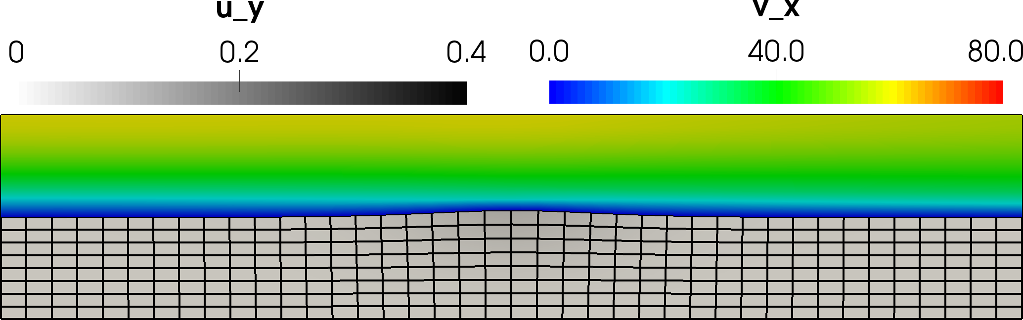
$t=100$ days

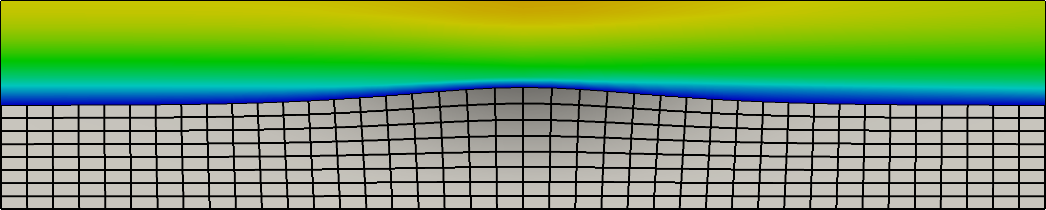
$t=200$ days

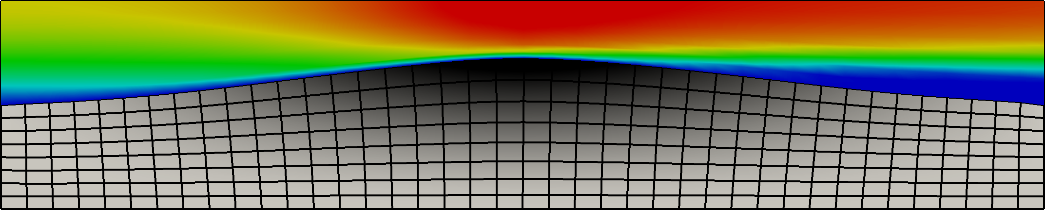
Figure 9: Visualization of the plaque growth at times $t=50$ days, $t=100$ days and $t=200$ days for the second numerical example (PDE growth model). The horizontal velocity (in cm/s) and the vertical displacement (in cm) are shown on the deformed domain at micro time $\tau=0.5$ s, i.e., the time of maximum inflow velocity. As the plaque growth evolves, significantly higher velocities arise in the central part.

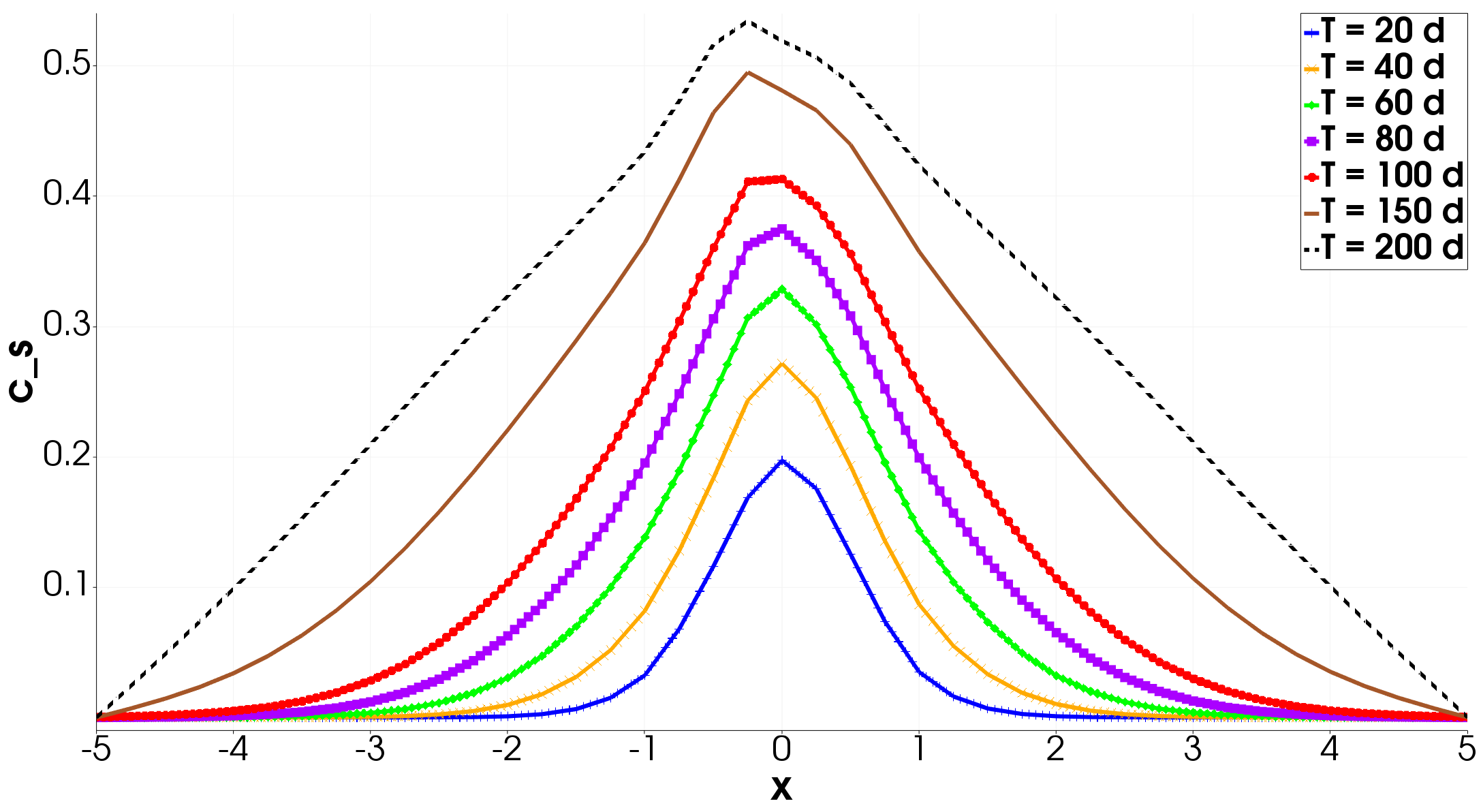
Figure 10: Foam cell concentration $\hat{c}_{s}$ at the FSI interface $\hat{\Gamma}$ at different times $t$ in the second numerical example (PDE growth model). In contrast to the ODE model, the concentration is not symmetric around the center anymore for larger times $t$; this is due to the reaction-diffusion equation.

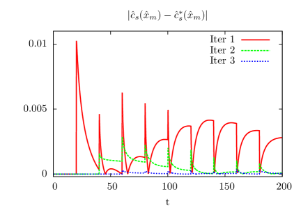
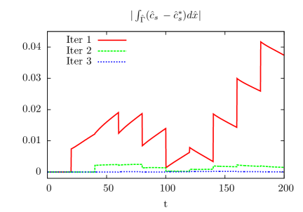
Figure 11: Errors for the second numerical example (PDE growth model) in different iterations of the parareal algorithm for $P=10$; the setting is described in section 5. Left: Error in the concentration $|\hat{c}_{s}^{(k),\text{fine}}(\hat{x}_{m},t)-\hat{c}_{s}^{*}(\hat{x}_{m},t)|$ at the midpoint of $\hat{\Gamma}$ over time; see also fig. 10 for the temporal evolution of $\hat{c}_{s}$ at the interface. Right: Error in the mean value $\big{|}\int_{\hat{\Gamma}}\hat{c}_{s}^{(k),\text{fine}}(\hat{x},t)-\hat{c}_{s}^{*}(\hat{x},t)\,\text{d}\hat{x}\big{|}$ over time.

k	$P=10$	$P=20$	$P=30$	$P=40$	$P=50$	ref. (serial)
1	$2.80\cdot 10^{-3}$	$1.42\cdot 10^{-3}$	$7.49\cdot 10^{-4}$	$6.53\cdot 10^{-4}$	$5.04\cdot 10^{-4}$	${0}$
2	$8.73\cdot 10^{-5}$	$9.46\cdot 10^{-5}$	$1.27\cdot 10^{-4}$	$6.22\cdot 10^{-5}$	$4.78\cdot 10^{-5}$
3	$3.45\cdot 10^{-5}$	$2.90\cdot 10^{-5}$	$2.97\cdot 10^{-5}$	$1.36\cdot 10^{-5}$	$9.19\cdot 10^{-6}$
4	-	$1.93\cdot 10^{-6}$	$4.45\cdot 10^{-6}$	-	-
Est. par.	11 347 s	9 661 s	8 692 s	6 914 s	7 491 s	26 840 s
speedup	2.4	2.8	3.1	3.9	3.6	1.0
efficiency	24 %	14 %	10 %	10 %	7 %	100 %

Table 4: Errors $|\hat{c}_{s}^{(k),{\text{fine}}}(T_{\text{end}})-\hat{c}_{s}^{*}(T_{\text{end}})|$ at the midpoint $\hat{x}_{m}$ of $\hat{\Gamma}$ for $P=10$ to $50$ for the parareal algorithm (algorithm 2) and a serial reference computation applied to the second numerical example (PDE growth model, $\hat{c}_{s}^{*}(T_{\text{end}})=0.5186632$). Estimated parallel runtimes are shown, as well as speedup and efficiency compared to the reference computation (right column). Details on the estimation of the runtimes are given in section 5.3. Best numbers are marked in bold face.

In the following section 5.1 we investigate numerically the convergence behavior of the standard parareal algorithm (algorithm 2) and the re-usage variant (algorithm 3). Then, we discuss the computational costs of the algorithms applied to the PDE growth model in section 5.2. Finally, we compare the algorithms in section 5.3 based on estimated runtimes of a parallel implementation.

5.1 Convergence behavior of the parallel time-stepping algorithms

We consider again the standard parareal algorithm (algorithm 2) and the modification with re-usage of growth values (algorithm 3). As stopping criterion, we now choose

$$|\hat{c}_{s}^{(k+1),{\text{fine}}}(\hat{x}_{m},T_{\text{end}})-\hat{c}_{s}^{(k),{\text{fine}}}(\hat{x}_{m},T_{\text{end}})|<\epsilon_{\text{par}}=10^{-4},$$

where $\hat{x}_{m}=(0,-1)$ is the center of the FSI interface $\hat{\Gamma}$, that is, a slightly more strict tolerance compared to the ODE model.

Standard parareal

In fig. 11, we show the evolution of the error in the first three iterates of the parareal algorithm over time for $P=N_{c}=10$. More precisely, we plot the error in the point functional $\hat{c}_{s}^{{(k),\text{fine}}}(\hat{x}_{m},t)$, that is, the foam cell concentration at the center of the FSI interface, and the average $\int_{\hat{\Gamma}}\hat{c}_{s}^{(k),\text{fine}}(\hat{x},t)\,\text{d}x$ of the foam cell concentration over time. As in the first numerical example, we observe fast convergence towards the reference values. Again, the foam cell concentrations $\hat{c}_{s}(\hat{x}_{m})$ are significantly overestimated in the initialization step, due to the large time-step $\delta T$ in step (I). These are the starting values for the fine problems in the first parareal iteration.

In table 4, we compare the convergence of the function values of $\hat{c}_{s}^{(k),\text{fine}}(\hat{x}_{m},T_{\text{end}})$ depending on the number of processes $P$. The findings are similar to the first numerical example (table 1). Again, depending on $P$, three to four parareal iterations were sufficient to reach the stopping criterion, with a slightly faster convergence behavior for larger $P$.

In table 5, we show numerical results for a fixed coarse time step $\delta T=\frac{T_{\text{end}}}{40}$, i.e., $N_{c}=40$ and varying $P\in\{10,20,40\}$. This means that the cost of the coarse propagator (in terms of the number of micro problems to be solved) is equal in all three cases. While the convergence behavior is slightly faster for smaller $P$, the stopping criterion was satisfied after 3 parareal iterations in all cases. As the fine propagator is cheaper for larger $P$, the fastest computation is $P=N_{c}=40$, with a speed-up of 4.3 in terms of the number of micro problems to be solved.

k	$P=10$	$P=20$	$P=40$	ref. (serial)
1	$8.51\cdot 10^{-4}$	$7.60\cdot 10^{-4}$	$6.53\cdot 10^{-4}$	0
2	$7.64\cdot 10^{-6}$	$2.25\cdot 10^{-5}$	$6.22\cdot 10^{-5}$	-
3	$4.36\cdot 10^{-7}$	$3.66\cdot 10^{-6}$	$1.36\cdot 10^{-5}$	-
# mp	460	310	235	1 000
speedup	2.2	3.2	4.3	1.0
efficiency	22 %	16 %	11 %	100 %

Table 5: Errors $|\hat{c}_{s}^{(k),{\text{fine}}}(T_{\text{end}})-\hat{c}_{s}^{*}(T_{\text{end}})|$ at the midpoint $\hat{x}_{m}$ of $\hat{\Gamma}$ for a fixed coarse time step ($N_{c}=40$), $P\in\{10,20,40\}$ and the parareal algorithm (algorithm 2) applied to the second numerical example (PDE growth model). Estimated parallel runtimes are shown, as well as speedup and efficiency compared to the reference computation (right column). Best numbers are marked in bold face.

Parareal with re-usage of growth values

In table 6, we show the results for the parareal algorithm with re-usage of growth values; cf. section 4.2.2. For all tested $P$, we need $k_{\text{par}}=5$ iterations to satisfy the stopping criterion. Similar to the first numerical example, these are 1-2 additional iterations compared to the standard parareal algorithm.

5.2 Theoretical discussion of the computational cost

While using the ODE growth model, it was obvious that the solution of the growth model and the communication could be neglected, this requires some discussion for the PDE growth model, as the reaction-diffusion equation eq. 33 needs to be solved to advance the foam cell concentration $\hat{c}_{s}$.

Standard parareal

In the standard parareal algorithm (algorithm 2), a time step of the PDE growth model always follows the solution of a micro problem, where the growth values $\gamma(\boldsymbol{\sigma}_{f}^{WS})$ are computed. Thus, the numbers of time steps of the PDE growth model and micro problems to be solved coincide. Considering that the latter consists of $\geq 100$ time steps, each involving the solution of a nonlinear, coupled FSI problem, while the growth model only requires the solution of a single scalar PDE of reaction-diffusion type, it is clear that the computational cost of the growth model is negligible.

Concerning communication, each process $p=1,...,P$ needs to communicate its final foam cell concentration ${\cal F}(\overline{c}_{s}^{(k)}(T_{p}))=\hat{c}_{s}^{(k),\text{fine}}(t_{p,n_{p}})$, which is a scalar-valued finite element function defined in the solid domain $\hat{{\cal S}}$, to the master process if the master-slave approach is used. No communication of ${\cal F}(\overline{c}_{s}^{k}(T_{p}))$ is required in a distributed approach; cf. section 4.1.1. Then, after the coarse propagator, the variables $\overline{c}_{s}^{(k+1)}(t_{p\cdot n_{p}})$ have to be communicated: in the master-slave approach, the data is transferred back to the slaves, and in the distributed case, it is communicated to the next process in line. Using the discretization outlined above, this corresponds to 369 degrees of freedom that need to be communicated each time.

As already discussed in section 4.1.1, in the master-slave case, this communication step is unfavorable because it involves all-to-one and one-to-all communication, whereas the communication pattern for the distributed parallelization only involves neighbor communication, which is more beneficial. However, in both cases, the two communication steps are only performed once during each parareal iteration. In order to investigate if the communication cost is still negligible for the PDE growth model, parallel numerical experiments based on an actual parallel implementation are needed, especially for realistic three-dimensional problems; see also the discussion in [34]. Due to the large computational cost of the micro problems in realistic three-dimensional problems, the communication cost might still be comparably small, which motivates the focus on the number of micro problems to be solved in our discussion; recall that, in our case, the micro problems consist of $\geq 100$ time steps of a fully coupled FSI problem. Obviously, this argumentation needs to be confirmed based on an actual parallel implementation; we will investigate this further in our future work.

Parareal with re-usage of growth values

The objective of the re-usage algorithm is to reduce the number of micro problems to be solved in the coarse-scale propagator. As this allows for a smaller time-step size $\delta t$ in the coarse problem, the number of reaction-diffusion equations to be solved, might increase significantly. Instead of $N_{c}$ of such equations in step (II.b)(i) of algorithm 2, algorithm 3 requires $N_{f}$ reaction-diffusion steps in step (II.b)(ii), where $N_{f}=1\,000$ in the example used in this section. Thus, in $k_{\text{par}}$ iterations of the parareal algorithm, the number of such equations to be solved is $k_{\text{par}}\cdot N_{f}$ in step (II.b)(ii) plus $N_{c}$ equations in step (I) and $k_{\text{par}}\cdot\lceil\frac{N_{f}}{P}\rceil$ in step (II.a)(ii) of algorithm 3. In total, algorithm 3 requires the solution of

$$k_{\text{par}}\cdot\left(N_{f}+\lceil N_{f}/P\rceil\right)+{N_{c}}$$

reaction-diffusion equations. For a comparison, we note that the number of micro problems to be solved for $P$ processes was $(k_{\text{par}}+1){N_{c}}+k_{\text{par}}\cdot\lceil N_{f}/P\rceil$ (see section 4.1.2). This means that the number of reaction-diffusion equations to be solved is by a factor

$$\frac{k_{\text{par}}\cdot\left(N_{f}+\lceil N_{f}/P\rceil\right)+{N_{c}}}{(k_{\text{par}}+1){N_{c}}+k_{\text{par}}\cdot\lceil N_{f}/P\rceil}$$

larger compared to the number of micro-problems. A simple calculation yields that

$$\frac{k_{\text{par}}\cdot\left(N_{f}+\lceil N_{f}/P\rceil\right)+{N_{c}}}{(k_{\text{par}}+1){N_{c}}+k_{\text{par}}\cdot\lceil N_{f}/P\rceil}\,\leq\,\frac{k_{\text{par}}\left(N_{f}+\lceil N_{f}/P\rceil+{N_{c}}\right)}{k_{\text{par}}\left({N_{c}}+\lceil N_{f}/P\rceil\right)}\,=\,\frac{N_{f}}{{N_{c}}+\lceil N_{f}/P\rceil}+1\,\leq\,\frac{\sqrt{N_{f}}}{2}+1.$$

In the last inequality, we have used that $N_{c}\geq P$. For $N_{f}=1\,000$, the bound on the right-hand side is approximately $16.8$.

Of course, another option would be to use coarser time steps for the coarse propagator. However, noting again that a micro problem consists of $\geq 100$ FSI steps, the computational cost for $\leq 16.8$ scalar reaction-diffusion equations is still much cheaper. This will be confirmed in the following section, where we show estimated runtimes of a parallel implementation and the respective contributions from the micro problems and the solves of reaction-diffusion equations.

For the re-usage of growth values and the distributed parallelization scheme, the communication cost does not change compared to the standard parareal algorithm. This is because the growth values to be re-used are already available on the process; this follows directly from the discussion in section 4.2.2. In the case, of master-slave communication, the communication cost is increased. In particular, $N_{f}$ growth functions $\overline{\gamma}_{i},i=1,...,N_{f}$ need to be transferred from the processes $p=1,...,P$ to the master process. Each $\overline{\gamma}_{i}$ is a spatially discretized function which is defined on the FSI interface $\hat{\Gamma}$. In the example considered here, it is non-zero only in the area $\hat{x}_{1}\in[-1,1]$ which corresponds to 7 degrees of freedom in our discretization; again, for a realistic three-dimensional problem, the number of degrees of freedom will increase drastically but will still remain small compared to the full problem size. As mentioned before, we assume that the communication cost is negligible compared to the solution of the micro problems in our discussion. Again, this assumption has to be tested in the future based on parallel results.

k	$P=10$	$P=20$	$P=30$	$P=40$	$P=50$	$P=60$	$P=70$	ref.
1	$2.80\cdot 10^{-3}$	$1.42\cdot 10^{-3}$	$7.49\cdot 10^{-4}$	$6.53\cdot 10^{-4}$	$5.04\cdot 10^{-4}$	$4.00\cdot 10^{-4}$	$3.32\cdot 10^{-4}$	0
2	$6.37\cdot 10^{-4}$	$6.96\cdot 10^{-4}$	$5.62\cdot 10^{-4}$	$4.08\cdot 10^{-4}$	$3.45\cdot 10^{-4}$	$3.09\cdot 10^{-4}$	$2.82\cdot 10^{-4}$
3	$1.33\cdot 10^{-4}$	$1.87\cdot 10^{-4}$	$2.06\cdot 10^{-4}$	$1.56\cdot 10^{-4}$	$1.39\cdot 10^{-4}$	$1.30\cdot 10^{-4}$	$1.25\cdot 10^{-4}$
4	$2.87\cdot 10^{-5}$	$5.31\cdot 10^{-5}$	$6.14\cdot 10^{-5}$	$5.08\cdot 10^{-5}$	$4.61\cdot 10^{-5}$	$4.29\cdot 10^{-5}$	$4.02\cdot 10^{-5}$
5	$5.05\cdot 10^{-6}$	$1.47\cdot 10^{-5}$	$1.67\cdot 10^{-5}$	$1.45\cdot 10^{-5}$	$1.20\cdot 10^{-5}$	$1.07\cdot 10^{-5}$	$1.05\cdot 10^{-5}$
Est. par.	17 733 s	9 685 s	7 105 s	5 902 s	5 277 s	4 925 s	4 804 s	26 840 s
speedup	1.5	2.8	3.8	4.5	5.1	5.4	5.6	1.0
efficiency	15 %	14 %	13 %	11 %	10 %	9 %	8 %	100 %

Table 6: Errors $|c_{s}^{(k),{\text{fine}}}(\hat{x}_{m},T_{\text{end}})-\hat{c}_{s}^{*}(\hat{x}_{m},T_{\text{end}})|$ at the midpoint $\hat{x}_{m}$ of $\hat{\Gamma}$ for $P=10$ to $70$ for algorithm 3 (Re-usage of growth values) applied to the second numerical example (PDE growth model). We show estimated parallel runtimes, as well as speedup and efficiency compared to the reference computation (right column). Details on the estimation of runtimes are given in section 5.3. Best numbers are marked in bold face.

5.3 Comparison of runtimes

The computational results given in this paper serve as a proof of concept to test the presented algorithms. From the discussion in the previous subsection, we assume that the only relevant computational cost comes from the solution of the micro problems. As mentioned before in our current implementation, we do not solve the fine-scale problems in parallel on different processes. Instead, they are solved sequentially one after the other on a single process. Since the cost for the micro problems dominates the computation times for any serial or parallel simulation of the plaque growth, we can still discuss the parallelization potential of the methods. The parallel implementation of the algorithms itself is subject to future work.

Figure 12: Illustration of the computational times spent within the coarse- (in serial) and fine-scale (in parallel) problems in algorithm 2 and algorithm 3 for the second numerical example (PDE growth problem)

Standard parareal (algorithm 2)
P coarse fine: max. (aver.) est. par. 10 1 096 s 10 251 s (8 009 s) 11 347 s 20 2 691 s 6 968 s (5 318 s) 9 661 s 30 3 943 s 4 749 s (3 581 s) 8 692 s 40 4 273 s 2 641 s (1 988 s) 6 914 s 50 5 361 s 2 130 s (1 601 s) 7 491 s 60 6 197 s 1 796 s (1 331 s) 7 993 s

Parareal with re-usage of growth values (algorithm 3)
P coarse fine: max. (aver.) est. par. 10 658 s 17 075 s (13 342 s) 17 733 s 20 930 s 8 755 s (6 669 s) 9 685 s 30 1 171 s 5 934 s (4 455 s) 7 105 s 40 1 448 s 4 454 s (3 339 s) 5 902 s 50 1 722 s 3 555 s (2 670 s) 5 277 s 60 1 933 s 2 992 s (2 219 s) 4 925 s

Table 7: Estimated parallel runtimes (in s) of the parareal algorithm and the variant "Re-usage of growth values" for $P=10,...,60$ and a PDE growth model. We show the time in seconds spent on the master process and the maximum and average time spent on the slave processes. The estimated parallel runtime is the sum of the time spent in serial (master) and the maximum time needed among the slaves; best numbers marked in bold face. A visualization of the runtimes is given in fig. 13. 

In this section, we will give an estimate of the runtimes that would be required in a parallel implementation. For this purpose, we list the serial part and parallel contributions of the computing times in table 7. The serial part corresponds to the coarse propagation, which is performed on a single master process (steps (I) and (II.b) in algorithm 2 or algorithm 3). The parallel part corresponds to the solution of the micro problems (step (II.a)). It can be performed concurrently on all processes $p=1,...,P$. The computing times vary slightly across the processes. It increases for larger processes $p$, as more Newton iterations are required for the FSI problem, when the channel is already significantly narrowed due to the advancing plaque growth. The estimated parallel runtimes given in tables 4, 6 and 7 are the sum of the serial part, which corresponds to the coarse propagator, and the maximum time needed by one of the processes $p=1,...,P$ in the parallel part.

Figure 13: Illustration of the computational times spent within micro-scale problems and PDE growth problems on the coarse (in serial) and fine scale (in parallel) in algorithm 2 and algorithm 3 for the second numerical example (PDE growth problem). Note that the time needed for the PDE growth model within the fine-scale problems is so small that it is not visible in both plots. The corresponding times can be found in table 7.

In fig. 12, we illustrate the computational times needed to solve the fine problems (in parallel) and coarse-scale propagators (in serial) for different processes and with algorithm 2 and algorithm 3. We see that the total computational times decrease for increasing $P$ until $P=40$ for standard parareal and until $P=60$ for the re-usage variant. In the standard parareal algorithm (algorithm 2) the cost of the coarse propagators becomes significant already from $P=20$, while it is much smaller for the re-usage variant. While for $P=10$, algorithm 2 is still faster, this changes for $P>20$.

The corresponding speed-ups and efficiencies compared to a serial time-stepping are given in the last rows of tables 4 and 6 for standard parareal algorithm (algorithm 2) and the re-usage variant (algorithm 3), respectively. The lowest computing time for standard parareal is 6 914 s for $P=40$, which corresponds to a speed-up of 3.9. For the re-usage variant, we obtain a maximum speed-up of 5.6 for $P=40$, which corresponds to an estimated parallel runtime of 4 804 s. The speed-ups are slightly lower than the speed-ups in section 4 (cf. tables 1 and 3), that were computed based on the number of micro problems to be solved. This is mostly due to the load imbalancing among the slave processes, as - depending on the state of the plaque growth - some micro problems are more costly than others; for instance, due to a higher number of Newton iterations. The differences can be inferred best by comparing the average and the maximum time spent on the slave processes in table 7. The efficiencies decrease again monotonically for increasing $P$ in both tables 4 and 6. For the re-usage variant, the efficiencies are again much more stable, due to the reduced cost of the coarse propagator.

Finally, we compare in fig. 13 the computing times needed for the solution of the FSI micro problems and those needed for the reaction-diffusion equations, for both algorithms and $P=10,...,60$. We observe that the times needed for the latter are negligible in all cases, which confirms the discussion in section 5.2.

6 Conclusion

We have derived a parareal algorithm for the time parallelization of the macro scale in a two-scale formulation for the simulation of atherosclerotic plaque growth. To reduce the computational cost of the coarse-scale propagators, we have introduced a variant which re-uses growth values that were computed within the fine problems and avoids additional costly micro-scale computations in serial.

The approaches have been tested on two different numerical examples of increasing complexity: first, by means of a simple ODE growth model, and secondly, by a PDE model of reaction-diffusion type. In this proof-of-concept, we analyze the approaches based on results and timings of a serial implementation. Since the number of communication steps is low compared to the computational work, we are still able to provide meaningful results. In the first case, we obtain estimated speedups up to 6.3 (standard parareal) respectively 7.8 (re-usage variant) in terms of the number of micro problems to be solved. In the PDE model, the maximum estimated speedups, now based on estimated parallel runtimes, were 3.9 respectively 5.6. In future work, these results will have to confirmed using a parallel implementation. Therefore, we have discussed theoretically two parallelization schemes, master-slave and distributed parallelization. The discussion indicated that the distributed scheme might be beneficial, which also needs to be tested in future work.

Additional research should also be invested into further improving the efficiency of the coarse propagator. Therefore, the idea of algorithm 3 could be extended, for example, by storing and interpolating the computed growth values, instead of simply re-using them. For the ODE case, such an interpolation approach has already been applied in our proceedings paper [53] with promising results. The extension to the PDE model is, however, not straight-forward, as an operator ${\cal M}:c_{s}\to\overline{\gamma}(\sigma_{f}^{WS}(c_{s}))$ between spatially distributed functions needs to be approximated. Further future investigations include the application of the algorithms in complex three-dimensional geometries, more complex plaque growth, and arterial wall models. Finally, the approaches presented here can be combined with a spatial parallelization of the FSI problems or with adaptive time-stepping on micro and macro scale, as presented by Richter & Lautsch [41].

Appendix

In this section, we show convergence of the re-usage parareal algorithm, algorithm 3 resp. eq. 28, applied to the ODE model in eq. 22 and its approximation by the explicit Euler method in eq. 23. First, we obtain from eqs. 23 and 24 directly for $c_{s}^{1},c_{s}^{2}\in\mathbb{R}$

$$|{\cal C}(I_{n},c_{s}^{1}(T_{n-1}),\gamma)-{\cal C}(I_{n},c_{s}^{2}(T_{n-1}),\gamma)| =|c_{s}^{1}(T_{n-1})-c_{s}^{2}(T_{n-1})|,$$ (35)

$$|{\cal C}(I_{n},c_{s},\gamma(c_{s}^{1}))-{\cal C}(I_{n},c_{s},\gamma(c_{s}^{2}))| =\delta T|\gamma(c_{s}^{1})-\gamma(c_{s}^{2})|\leq L\delta T|c_{s}^{1}-c_{s}^{2}|.$$ (36)

By $c_{s,n-1}(T)$ we denote in the following the function that solves the (continuous) ODE eq. 22 with initial value $c_{s,n-1}(T_{n-1})=c_{s,n-1}$. We have using eqs. 23, 24 and 25

$$\begin{split}&\Big{|}\left({\cal F}(I_{n},c_{s}(T_{n-1}),\gamma(c_{s}(T_{n-1})))-{\cal C}(I_{n},c_{s}(T_{n-1}),\gamma(c_{s}(T_{n-1})))\right)\\ &\qquad-\left({\cal F}(I_{n},c_{s,n-1},\gamma(c_{s,n-1}))-{\cal C}(I_{n},c_{s,n-1},\gamma(c_{s,n-1}))\right)\Big{|}\\ &=\Big{|}\int_{T_{n-1}}^{T_{n}}\gamma(c_{s}(T)))-\gamma(c_{s,n-1}(T))\,\text{d}T-\delta T\left(\gamma(c_{s}(T_{n-1}))-\gamma(c_{s,n-1})\right)\Big{|}\\ &\leq c\delta T^{2}\left|{\frac{d}{dt}}\gamma(c_{s}(T_{n-1})-{\frac{d}{dt}}\gamma(c_{s,n-1})\right|\leq\alpha_{0}\delta T^{2}\left|c_{s}(T_{n-1})-c_{s,n-1}\right|\end{split}$$ (37)

for some constant $\alpha_{0}=cL>0$; see also [32].

The following recursion builds the basis for the error estimate:

Lemma 2.

Let $c_{s}^{*}\in C^{1}(0,T_{\text{end}})$ be the exact solution of eq. 22. $\{\overline{c}_{s}^{(k)}(T_{n})\}_{n=1}^{P}$ be the $k$-th iterate of the re-usage algorithm in eq. 28 using the forward Euler method in eq. 23 and let $e_{n}^{(k)}=|c_{s}^{*}(T_{n})-\overline{c}_{s,n}^{(k)}|$ be the error in the $k$-the iteration of the re-usage algorithm. Under the assumptions made in section 4.1.3, it holds for $k=1$ that

$$e_{n}^{(1)} \leq\alpha_{0}\delta T^{2}e_{n-1}^{(0)}+\alpha_{1}\delta Te_{n-2}^{(0)}+e_{n-1}^{(1)},$$ (38)

and for $k\geq 2$,

$$e_{n}^{(k)} \leq\alpha_{1}\delta T\left(e_{n-1}^{(k-1)}+e_{n-2}^{(k-1)}+e_{n-2}^{(k-2)}\right)+e_{n-1}^{(k)},$$ (39)

with a constant $\alpha_{1}\geq\max\{L+\alpha_{0}\delta T,L(1+L\delta T)\}$.

Proof.

Consider first the case $k\geq 2$. Using eqs. 28 and 25, we have

$$e_{n}^{(k)} =\big{|}{\cal F}(I_{n},c_{s}^{*}(T_{n-1}),\gamma(c_{s}^{*}(T_{n-1}))-{\cal C}(I_{n},\overline{c}_{s,n-1}^{(k)},\gamma(c_{s,n-1}^{(k),\text{fine}}))$$

$$\qquad-{\cal F}(I_{n},\overline{c}_{s,n-1}^{(k-1)},\gamma(\overline{c}_{s,n-1}^{(k-1)}))+{\cal C}(I_{n},\overline{c}_{s,n-1}^{(k-1)},\gamma(c_{s,n-1}^{(k-1),\text{fine}}))\big{|}$$

$$\leq\big{|}{\cal F}(I_{n},c_{s}^{*}(T_{n-1}),\gamma(c_{s}^{*}(T_{n-1})))-{\cal C}(I_{n},c_{s}^{*}(T_{n-1}),\gamma(c_{s}^{*}(T_{n-1})))$$

$$\qquad-{\cal F}(I_{n},\overline{c}_{s,n-1}^{(k-1)},\gamma(\overline{c}_{s,n-1}^{(k-1)}))+{\cal C}(I_{n},\overline{c}_{s,n-1}^{(k-1)},\gamma(\overline{c}_{s,n-1}^{(k-1)}))\big{|}$$

$$\quad+\big{|}{\cal C}(I_{n},\overline{c}_{s,n-1}^{(k-1)},\gamma(\overline{c}_{s,n-1}^{(k-1)}))-{\cal C}(I_{n},\overline{c}_{s,n-1}^{(k-1)},\gamma(c_{s,n-1}^{(k-1),\text{fine}}))\big{|}$$

$$\quad+\big{|}{\cal C}(I_{n},\overline{c}_{s,n-1}^{(k)},\gamma(c_{s,n-1}^{(k),\text{fine}}))-{\cal C}(I_{n},\overline{c}_{s,n-1}^{(k)},\gamma(c_{s}^{*}(T_{n-1})))\big{|}$$

$$\quad+\big{|}{\cal C}(I_{n},\overline{c}_{s,n-1}^{(k)},\gamma(c_{s}^{*}(T_{n-1})))-{\cal C}(I_{n},c_{s}^{*}(T_{n-1}),\gamma(c_{s}^{*}(T_{n-1})))\big{|}$$

From eqs. 35, 36 and LABEL:long1, we have

$$\begin{split}e_{n}^{(k)}&\leq\alpha_{0}\delta T^{2}\left|c_{s}^{*}(T_{n-1})-\overline{c}_{s,n-1}^{(k-1)}\right|+L\delta T\big{|}\overline{c}_{s,n-1}^{(k-1)}-c_{s,n-1}^{(k-1),\text{fine}}\big{|}\\ &\quad+L\delta T\big{|}c_{s,n-1}^{(k),\text{fine}}-c_{s}^{*}(T_{n-1})\big{|}+\big{|}\overline{c}_{s,n-1}^{(k)}-c_{s}^{*}(T_{n-1})\big{|}\\ &=\alpha_{0}\delta T^{2}e_{n-1}^{(k-1)}+L\delta T(e_{n-1}^{(k-1),\text{fine}}+e_{n-1}^{(k-1)})+L\delta Te_{n-1}^{(k),\text{fine}}+e_{n-1}^{(k)},\end{split}$$ (40)

where $e_{n-1}^{(k),\text{fine}}:=|c_{s,n-1}^{(k),\text{fine}}-c_{s}^{*}(T_{n})|$. This error contribution is estimated further by using eqs. 29, 25 and 35

$$\begin{split}e_{n-1}^{(k),\text{fine}}:=|c_{s,n-1}^{(k),\text{fine}}-c_{s}^{*}(T_{n})|&=|{\cal F}(I_{n-1},c_{s,n-2}^{(k-1)},\gamma(c_{s,n-2}^{(k-1)}))-{\cal F}(I_{n-1},c_{s}^{*}(T_{n-2}),\gamma(c_{s}^{*}(T_{n-2}))|\\ &=\big{|}c_{s,n-2}^{(k-1)}-c_{s}^{*}(T_{n-2})+\int_{T_{n-2}}^{T_{n-1}}\gamma(c_{s,n-2}^{(k-1)}(t)))-\gamma(c_{s}^{*}(t))\,\text{d}t\big{|}\\ &\leq(1+L\delta T)e_{n-2}^{(k-1)}.\end{split}$$ (41)

Inserting this into eq. 40 yields eq. 39. For $k=1$, we have $c_{s,n-1}^{(0),\text{fine}}=c_{s,n-1}^{(0)}$. An analogous argumentation yields

$$e_{n}^{(1)} =\big{|}{\cal F}(I_{n},c_{s}^{*}(T_{n-1}),\gamma(c_{s}^{*}(T_{n-1})))-{\cal C}(I_{n},\overline{c}_{s,n-1}^{(1)},\gamma(c_{s,n-1}^{(1),\text{fine}}))$$

$$\qquad-{\cal F}(I_{n},\overline{c}_{s,n-1}^{(0)},\gamma(\overline{c}_{s,n-1}^{(0)}))+{\cal C}(I_{n},\overline{c}_{s,n-1}^{(0)},\gamma(c_{s,n-1}^{(0)}))\big{|}$$

$$\leq\big{|}{\cal F}(I_{n},c_{s}^{*}(T_{n-1}),\gamma(c_{s}^{*}(T_{n-1})))-{\cal C}(I_{n},c_{s}^{*}(T_{n-1}),\gamma(c_{s}^{*}(T_{n-1})))$$

$$\qquad-{\cal F}(I_{n},\overline{c}_{s,n-1}^{(0)},\gamma(\overline{c}_{s,n-1}^{(0)}))+{\cal C}(I_{n},\overline{c}_{s,n-1}^{(0)},\gamma(\overline{c}_{s,n-1}^{(0)}))\big{|}$$

$$\quad+\big{|}{\cal C}(I_{n},\overline{c}_{s,n-1}^{(1)},\gamma(c_{s,n-1}^{(1),\text{fine}}))-{\cal C}(I_{n},\overline{c}_{s,n-1}^{(1)},\gamma(c_{s}^{*}(T_{n-1})))\big{|}$$

$$\quad+\big{|}{\cal C}(I_{n},\overline{c}_{s,n-1}^{(1)},\gamma(c_{s}^{*}(T_{n-1})))-{\cal C}(I_{n},c_{s}^{*}(T_{n-1}),\gamma(c_{s}^{*}(T_{n-1})))\big{|}$$

$$\leq\alpha_{0}\delta T^{2}e_{n-1}^{(0)}+L\delta Te_{n-1}^{(1),\text{fine}}+e_{n-1}^{(1)}.$$

Then, eq. 38 follows by using eq. 41. ∎

Lemma 3.

Let $e_{n}^{(k)}=|\overline{c}_{s}^{(k)}(T_{n})-c_{s}^{*}(T_{n})|$ be the error in the $k$-the iteration of the re-usage algorithm. Under the assumptions made above, it holds for $k\in\mathbb{N}_{0}$ and $n\in\mathbb{N}$ that

$$e_{n}^{(k)} \leq L\tilde{\alpha}^{k}\beta^{n-k}\cdot\left(\sum_{l=\lceil\frac{k}{2}+1\rceil}^{k+1}\frac{3^{l-1}}{l!}\delta T^{l+1}\left(n-\frac{k}{2}\right)^{l}\right)\max_{t\in[0,T_{\text{end}}]}|\partial_{t}c_{s}^{*}(t)|$$ (42)

$$\leq L\tilde{\alpha}^{k}\beta^{n-k}\delta T\max\left\{1,T_{n-\frac{k}{2}}\right\}^{k}\frac{3^{\lceil\frac{k}{2}\rceil}}{\lceil\nicefrac{{k}}{{2}}\rceil!}\max_{t\in[0,T_{\text{end}}]}|\partial_{t}c_{s}^{*}(t)|,$$ (43)

where $\tilde{\alpha}=\max\{\alpha_{0}\delta T,\alpha_{1},1\}$ and $\beta=1+L\delta T$.

Proof.

We prove the lemma by induction over $k\in\mathbb{N}$. For $k=0$, a standard estimate of the forward Euler methods gives, using eq. 24,

$$\begin{split}e_{n}^{(0)}:=|c_{s,n}^{0}-c_{s}^{*}(T_{n})|&\leq|c_{s,n-1}^{0}-c_{s}^{*}(T_{n-1})|+\int_{T_{n-1}}^{T_{n}}|\gamma(c_{s,n-1}^{0})-\gamma(c_{s}^{*}(t))|\,\text{d}t\\ &\leq e_{n-1}^{(0)}+L\int_{T_{n-1}}^{T_{n}}|c_{s,n-1}^{0}-\underbrace{c_{s}^{*}(t)}_{=c_{s}^{*}(T_{n-1})+\delta T\partial_{t}c_{s}^{*}(\xi)|}|\,\text{d}t\\ &\leq(\underbrace{1+L\delta T}_{=\beta})e_{n-1}^{(0)}+L\delta T^{2}\max_{t\in[0,T_{\text{end}}]}|\partial_{t}c_{s}^{*}(t)|.\end{split}$$ (44)

To abbreviate the notation, we set $c_{0}:=\max_{t\in[0,T_{\text{end}}]}|\partial_{t}c_{s}^{*}(t)|$. We apply eq. 44 recursively

$$e_{n}^{(0)}\leq\beta e_{n-1}^{(0)}+c_{0}L\delta T^{2}\leq c_{0}L\delta T^{2}\sum_{l=0}^{n-1}\beta^{l}=c_{0}L\delta T^{2}\frac{\beta^{n}-1}{\underbrace{\beta-1}_{=L\delta T}} =c_{0}\delta T(\beta^{n}-1)\leq c_{0}Ln\delta T^{2}\beta^{n}.$$ (45)

In the last inequality, we have used that $\beta^{n}-1\leq nL\delta T\beta^{n}$, which can be shown by induction over $n$. The estimate in eq. 45 is exactly eq. 42 for $k=0$.

For $k=1$, we have using eqs. 38 and 45, the fact that $e_{k}^{(k)}=0$, and by the definition of the parareal algorithm

$$e_{n}^{(1)} \leq\alpha_{0}\delta T^{2}e_{n-1}^{(0)}+\alpha_{1}\delta Te_{n-2}^{(0)}+e_{n-1}^{(1)}$$

$$\leq\alpha_{0}c_{0}L\delta T^{4}(n-1)\beta^{n-1}+\alpha_{1}c_{0}L\delta T^{3}(n-2)\beta^{n-2}+e_{n-1}^{(1)}$$

$$\leq 2\tilde{\alpha}c_{0}L\delta T^{3}(n-1)\beta^{n-1}+e_{n-1}^{(1)}$$

$$\leq 2\tilde{\alpha}c_{0}L\beta^{n-1}\delta T^{3}\sum_{l=1}^{n-1}l+\underbrace{e_{1}^{(1)}}_{=0}$$

$$=2\tilde{\alpha}c_{0}L\beta^{n-1}\delta T^{3}\frac{n(n-1)}{2}\leq\tilde{\alpha}c_{0}L\beta^{n-1}\delta T^{3}\left(n-\nicefrac{{1}}{{2}}\right)^{2}.$$

This is by a factor $\frac{3}{2}$ smaller compared to eq. 42.

Now, let $k\geq 2$. We assume that the estimate in eq. 42 is true for $k-1$ and $k-2$. By eq. 39 and the assumption of the induction, we have

$$\begin{split}e_{n}^{(k)}&\leq\alpha_{1}\delta T\left(e_{n-1}^{(k-1)}+e_{n-2}^{(k-1)}+e_{n-2}^{(k-2)}\right)+e_{n-1}^{(k)}\\ &\leq\alpha_{1}\delta T\Bigg{(}c_{0}L\tilde{\alpha}^{k-1}\beta^{n-k}\cdot\left(\sum_{l=\lceil\frac{k+1}{2}\rceil}^{k}\frac{3^{l-1}}{l!}\delta T^{l+1}\left(n-\frac{k+1}{2}\right)^{l}\right)\\ &\qquad\qquad+c_{0}L\tilde{\alpha}^{k-1}\beta^{n-k-1}\cdot\left(\sum_{l=\lceil\frac{k+1}{2}\rceil}^{k}\frac{3^{l-1}}{l!}\delta T^{l+1}\left(n-1-\frac{k+1}{2}\right)^{l}\right)\\ &\qquad\qquad+c_{0}L\tilde{\alpha}^{k-2}\beta^{n-k}\cdot\left(\sum_{l=\lceil\frac{k}{2}\rceil}^{k-1}\frac{3^{l-1}}{l!}\delta T^{l+1}\left(n-1-\frac{k}{2}\right)^{l}\right)\Bigg{)}\,\,+e_{n-1}^{(k)}\\ &\leq 3c_{0}L\tilde{\alpha}^{k}\beta^{n-k}\cdot\left(\sum_{l=\lceil\frac{k}{2}\rceil}^{k}\frac{3^{l-1}}{l!}\delta T^{l+2}\left(n-\frac{k+1}{2}\right)^{l}\right)+e_{n-1}^{(k)}.\end{split}$$ (46)

We apply this estimate recursively for the last term $e_{n-1}^{(k)}$ in eq. 46 to get

$$e_{n}^{(k)} \leq c_{0}L\tilde{\alpha}^{k}\beta^{n-k}\cdot\sum_{m=k+1}^{n}\left(\sum_{l=\lceil\frac{k}{2}\rceil}^{k}\frac{3^{l}}{l!}\delta T^{l+2}\left(m-\frac{k+1}{2}\right)^{l}\right)+\underbrace{e_{k}^{(k)}}_{=0}$$

$$=c_{0}L\tilde{\alpha}^{k}\beta^{n-k}\cdot\left(\sum_{l=\lceil\frac{k}{2}\rceil}^{k}\frac{3^{l}}{l!}\delta T^{l+2}\cdot\underbrace{\left(\sum_{m=\frac{k+1}{2}}^{n-\frac{k+1}{2}}m^{l}\right)}_{=:s}\right).$$

In the case that $\frac{k+1}{2}$ and $n-\frac{k+1}{2}$ are no natural number, the sum $s$ is to be understood in such a way that the index $m$ advances iteratively by 1 until reaching the upper limit.

The sum $s$ is an approximation of the integral

$$\int_{\nicefrac{{k}}{{2}}}^{n-\nicefrac{{k}}{{2}}}x^{l}\,\text{d}x\leq\frac{1}{l+1}\left(n-\frac{k}{2}\right)^{l+1}$$

with the midpoint rule. As $f(x)=x^{l}$ is a convex function ($f^{\prime\prime}(x)>0$) for a positive $x$, the integral is an upper bound for $s$; see the error representation of the midpoint rule, e.g., in Theorem 8.41 in [49].

We have thus shown that

$$e_{n}^{(k)}\leq c_{0}L\tilde{\alpha}^{k}\beta^{n-k}\cdot\left(\sum_{l=\lceil\frac{k}{2}\rceil}^{k}\frac{3^{l}}{(l+1)!}\delta T^{l+2}\left(n-\frac{k}{2}\right)^{l+1}\right).$$

Shifting the index $l$ by 1 gives eq. 42. The estimate in eq. 43 follows from eq. 42 by noting that

$$(n-\frac{k}{2})\delta T=T_{n-\frac{k}{2}}\leq\max\left\{1,T_{n-\frac{k}{2}}\right\}$$

and the fact that the term $\frac{3^{l-1}}{l!}$ is decreasing for $l\geq 2$:

$$e_{n}^{(k)} \leq c_{0}L\tilde{\alpha}^{k}\beta^{n-k}\cdot\left(\sum_{l=\lceil\frac{k}{2}+1\rceil}^{k+1}\frac{3^{l-1}}{l!}\delta T^{l+1}\left(n-\frac{k}{2}\right)^{l}\right)$$

$$\leq c_{0}L\tilde{\alpha}^{k}\beta^{n-k}\delta T\left(\max\{1,T_{n-\frac{k}{2}}\}\right)^{k+1}\cdot\left(\sum_{l=\lceil\frac{k}{2}+1\rceil}^{k+1}\frac{3^{l-1}}{l!}\right)$$

$$\leq c_{0}L\tilde{\alpha}^{k}\beta^{n-k}\delta T\left(\max\left\{1,T_{n-\frac{k}{2}}\right\}\right)^{k+1}\lfloor\frac{k}{2}+1\rfloor\frac{3^{\lceil\frac{k}{2}\rceil}}{\lceil\frac{k}{2}+1\rceil!}$$

$$\leq c_{0}L\tilde{\alpha}^{k}\beta^{n-k}\delta T\left(\max\left\{1,T_{n-\frac{k}{2}}\right\}\right)^{k+1}\frac{3^{\lceil\frac{k}{2}\rceil}}{\lceil\frac{k}{2}\rceil!}.$$

∎

References

- [1] A. Abdulle, W. E, B. Engquist, and E. Vanden-Eijnden. The heterogeneous multiscale method. Acta Numerica, pages 1–87, 2012.
- [2] C Ager, B Schott, AT Vuong, A Popp, and WA Wall. A consistent approach for fluid-structure-contact interaction based on a porous flow model for rough surface contact. Int J Numer Methods Eng, 119(13):1345–1378, 2019.
- [3] UM Ascher, SJ Ruuth, and BTR Wetton. Implicit-explicit methods for time-dependent partial differential equations. SIAM J Numer Anal, 32(3):797–823, 1995.
- [4] Eric Aubanel. Scheduling of tasks in the parareal algorithm. Parallel Computing, 37(3):172–182, March 2011.
- [5] D. Balzani, S. Deparis, S. Fausten, D. Forti, A. Heinlein, A. Klawonn, A. Quarteroni, O. Rheinbach, and J. Schröder. Numerical modeling of fluid-structure interaction in arteries with anisotropic polyconvex hyperelastic and anisotropic viscoelastic material models at finite strains. Int J Numer Method Biomed Eng, 32(10):e02756, 2016.
- [6] D. Balzani, S. Deparis, S. Fausten, D. Forti, A. Heinlein, A. Klawonn, A. Quarteroni, O. Rheinbach, and Jörg Schröder. Aspects of arterial wall simulations: Nonlinear anisotropic material models and fluid structure interaction. In Joint 11th WCCM, 5th ECCM and 6th ECFD 2014, pages 947–958, 2014.
- [7] D. Balzani, A. Heinlein, A. Klawonn, O. Rheinbach, and J. Schröder. Comparison of arterial wall models in fluid–structure interaction simulations. Accepted for publication in Computational Mechnanics. March 2023.
- [8] D. Balzani, P. Neff, J. Schröder, and G. A. Holzapfel. A polyconvex framework for soft biological tissues. adjustment to experimental data. Int J Solids Struct, 43(20):6052–6070, 2006.
- [9] A. T Barker and X.-C. Cai. Scalable parallel methods for monolithic coupling in fluid–structure interaction with application to blood flow modeling. J Comp Phys, 229(3):642–659, 2010.
- [10] Y. Bazilevs, K. Takizawa, and T. E. Tezduyar. Computational Fluid-Structure Interaction: Methods and Applications. Wiley Series in Computational Mechanics. Wiley, 2013.
- [11] R. Becker and M. Braack. A finite element pressure gradient stabilization for the Stokes equations based on local projections. Calcolo, 38(4):173–199, 2001.
- [12] R. Becker, M. Braack, D. Meidner, T. Richter, and B. Vexler. The finite element toolkit Gascoigne3d. http://www.gascoigne.de.
- [13] Dominik Brands, A. Klawonn, O. Rheinbach, and Jörg Schröder. Modelling and convergence in arterial wall simulations using a parallel feti solution strategy. Comput Methods Biomech Biomed Engin, 11(5):569–583, 2008.
- [14] E. Burman, M.A. Fernández, and S. Frei. A Nitsche-based formulation for fluid-structure interactions with contact. ESAIM: M2AN, 54(2):531–564, 2020.
- [15] E. Burman, M.A. Fernández, S. Frei, and F.M. Gerosa. A mechanically consistent model for fluid-structure interactions with contact including seepage. Comput Methods Appl Mech Eng, 2022. accepted for publication. arXiv pre-print: https://arxiv.org/abs/2103.11243.
- [16] LJ Caucha, S Frei, and O Rubio. Finite element simulation of fluid dynamics and CO2 gas exchange in the alveolar sacs of the human lung. Comput Appl Math, 37(5):6410–6432, 2018.
- [17] C.X. Chen, Y. Ding, and J.A. Gear. Numerical simulation of atherosclerotic plaque growth using two-way fluid-structural interaction. ANZIAM J., 53:278–291, 2012.
- [18] P. Crosetto, S. Deparis, G. Fourestey, and A. Quarteroni. Parallel algorithms for fluid-structure interaction problems in haemodynamics. SIAM J Sci Comp, 33(4):1598–1622, 2011.
- [19] S. Deparis, D. Forti, G. Grandperrin, and A. Quarteroni. Facsi: A block parallel preconditioner for fluid–structure interaction in hemodynamics. J Comp Phys, 327:700–718, 2016.
- [20] S. S. Dhawan, R. P. Avati Nanjundappa, J. R. Branch, W. R. Taylor, A. A. Quyyumi, H. Jo, M. C. McDaniel, J. Suo, D. Giddens, and H. Samady. Shear stress and plaque development. Expert review of cardiovascular therapy, 8(4):545–556, 2010.
- [21] J. Donea, A. Huerta, J.-P. Ponthot, and A. Rodríguez-Ferran. Arbitrary Lagrangian–Eulerian Methods, chapter 14. John Wiley & Sons, Ltd, 2004.
- [22] T. Dunne. An Eulerian approach to fluid-structure interaction and goal-oriented mesh refinement. Int J Numer Methods Fluids, 51:1017–1039, 2006.
- [23] W. E. Principles of Multiscale Modeling. Cambridge University Press, 2011.
- [24] W. E and B. Engquist. The heterogenous multiscale method. Comm. Math. Sci., 1(1):87–132, 2003.
- [25] CA Figueroa, S Baek, CA Taylor, and JD Humphrey. A computational framework for fluid–solid-growth modeling in cardiovascular simulations. Comput Methods Appl Mech Eng, 198(45-46):3583–3602, 2009.
- [26] L. Formaggia, A. Quarteroni, and A. Veneziani. Cardiovascular Mathematics: Modeling and simulation of the circulatory system, volume 1. Springer Science & Business Media, 2010.
- [27] S Frei. Eulerian finite element methods for interface problems and fluid-structure interactions. PhD thesis, Heidelberg University, 2016. http://www.ub.uni-heidelberg.de/archiv/21590.
- [28] S Frei, A Heinlein, and T Richter. On temporal homogenization in the numerical simulation of atherosclerotic plaque growth. PAMM, 21(1):e202100055, 2021.
- [29] S. Frei and T. Richter. Efficient approximation of flow problems with multiple scales in time. SIAM J Multiscale Model Simul, 18(2):942–969, 2020.
- [30] S. Frei, T. Richter, and T. Wick. Long-term simulation of large deformation, mechano-chemical fluid-structure interactions in ALE and fully Eulerian coordinates. J Comput Phys, 321:874 – 891, 2016.
- [31] M. J. Gander. 50 years of Time Parallel Time Integration. In Multiple Shooting and Time Domain Decomposition. Springer, 2015.
- [32] Martin J. Gander and Ernst Hairer. Nonlinear convergence analysis for the parareal algorithm. In Ulrich Langer, Marco Discacciati, David E. Keyes, Olof B. Widlund, and Walter Zulehner, editors, Domain Decomposition Methods in Science and Engineering XVII, pages 45–56. Springer Berlin Heidelberg, 2008.
- [33] M. W Gee, U. Küttler, and W. A. Wall. Truly monolithic algebraic multigrid for fluid–structure interaction. Int J Numer Methods Eng, 85(8):987–1016, 2011.
- [34] Sebastian Götschel, Michael Minion, Daniel Ruprecht, and Robert Speck. Twelve Ways to Fool the Masses When Giving Parallel-in-Time Results. In Benjamin Ong, Jacob Schroder, Jemma Shipton, and Stephanie Friedhoff, editors, Parallel-in-Time Integration Methods, Springer Proceedings in Mathematics & Statistics, pages 81–94, Cham, 2021. Springer International Publishing.
- [35] A. Heinlein, A. Klawonn, and O. Rheinbach. A parallel implementation of a two-level overlapping Schwarz method with energy-minimizing coarse space based on Trilinos. SIAM J Sci Comp, 38(6):C713–C747, 2016.
- [36] A. Heinlein, A. Klawonn, and O. Rheinbach. Parallel two-level overlapping schwarz methods in fluid-structure interaction. In Proceedings of ENUMATH 2015, pages 521–530. Springer, 2016.
- [37] G. A. Holzapfel, T. C. Gasser, and R. W. Ogden. A new constitutive framework for arterial wall mechanics and a comparative study of material models. J Elast, 61(1):1–48, 2000.
- [38] J. Hron and S. Turek. A monolithic FEM/multigrid solver for an ALE formulation of fluid-structure interaction with applications in biomechanics. In Fluid-structure interaction, pages 146–170. Springer, 2006.
- [39] F. Kong and X.-C. Cai. Scalability study of an implicit solver for coupled fluid-structure interaction problems on unstructured meshes in 3d. Int J High Perform Comput Appl, 32(2):207–219, 2018.
- [40] U. Küttler, M. Gee, C. Förster, A. Comerford, and W. A. Wall. Coupling strategies for biomedical fluid–structure interaction problems. Int J Numer Methods Biomed Eng, 26(3-4):305–321, 2010.
- [41] L. Lautsch and T. Richter. Error estimation and adaptivity for differential equations with multiple scales in time. Comput Methods Appl Math, 2021.
- [42] J.-L. Lions, Y. Maday, and G. Turinici. A "parareal" in time discretization of PDE’s. Comptes Rendus de l’Académie des Sciences - Series I - Mathematics, 332:661–668, 2001.
- [43] Margenberg, N. and Richter, T. Parallel time-stepping for fluid-structure interactions. Math. Model. Nat. Phenom., 16:20, 2021.
- [44] J Mizerski and T Richter. The candy wrapper problem-a temporal multiscale approach for pde/pde systems. In Proceedings of ENUMATH 2019, 2019.
- [45] Benjamin W. Ong and Jacob B. Schroder. Applications of time parallelization. Computing and Visualization in Science, 23(1-4):Paper No. 11, 15, 2020.
- [46] S Pozzi, A Redaelli, C Vergara, E Votta, and P Zunino. Mathematical modeling and numerical simulation of atherosclerotic plaque progression based on fluid-structure interaction. J Math Fluid Mech, 23(3):1–21, 2021.
- [47] T. Richter. A fully Eulerian formulation for fluid-structure interactions. J Comput Phys, 233:227–240, 2013.
- [48] T. Richter. Finite Elements for Fluid-Structure Interactions. Models, Analysis and Finite Elements., volume 118 of Lecture Notes in Computational Science and Engineering. Springer, 2017.
- [49] Thomas Richter and Thomas Wick. Einführung in die Numerische Mathematik: Begriffe, Konzepte und zahlreiche Anwendungsbeispiele. Springer-Verlag, 2017.
- [50] E.K. Rodriguez, A. Hoger, and A. D. McCulloch. Stress-dependent finite growth in soft elastic tissues. J. Biomech., 4:455–467, 1994.
- [51] D Ruprecht. Wave propagation characteristics of parareal. Comput Vis Sci, 19(1):1–17, 2018.
- [52] Daniel Ruprecht. Shared memory pipelined parareal. In Euro-Par 2017: Parallel Processing: 23rd International Conference on Parallel and Distributed Computing, Santiago de Compostela, Spain, August 28–September 1, 2017, Proceedings 23, pages 669–681. Springer, 2017.
- [53] A. Heinlein S. Frei. Efficient coarse correction for parallel time-stepping in plaque growth simulations. In Proceedings of the 8th ECCOMAS Congress, 2022. https://www.scipedia.com/public/Frei_et_al_2022a.
- [54] T. Silva, W. Jäger, M. Neuss-Radu, and A. Sequeira. Modeling of the early stage of atherosclerosis with emphasis on the regulation of the endothelial permeability. J Theor Biol, 496:110229, 2020.
- [55] F. Sonner. Temporal Multiscale Methods for a Model of Atherosclerosis. PhD thesis, FAU Erlangen-Nürnberg, 2021.
- [56] MP Thon, A Hemmler, A Glinzer, M Mayr, M Wildgruber, A Zernecke-Madsen, and MW Gee. A multiphysics approach for modeling early atherosclerosis. Biomech Model Mechanobiol, 17(3):617–644, 2018.
- [57] A. Wahle, J. J. Lopez, M. E. Olszewski, S. C. Vigmostad, K. B. Chandran, J. D. Rossen, and M. Sonka. Plaque development, vessel curvature, and wall shear stress in coronary arteries assessed by x-r. angiography and intravascular ultrasound. Medical image analysis, 10(4):615–631, 2006.
- [58] Y. Wu and X.-C. Cai. A fully implicit domain decomposition based ale framework for three-dimensional fluid–structure interaction with application in blood flow computation. J Comp Phys, 258:524–537, 2014.
- [59] Y. Yang, W. Jäger, M. Neuss-Radu, and T. Richter. Mathematical modeling and simulation of the evolution of plaques in blood vessels. J Math Biol, pages 1–24, 2014.
- [60] Y. Yang, T. Richter, W. Jäger, and M. Neuss-Radu. An ALE approach to mechano-chemical processes in fluid-structure interactions. Int J Numer Methods Fluids, 84(4):199–220, 2017.