Quantum Motion Segmentation

Abstract

Motion segmentation is a challenging problem that seeks to identify independent motions in two or several input images. This paper introduces the first algorithm for motion segmentation that relies on adiabatic quantum optimization of the objective function. The proposed method achieves on-par performance with the state of the art on problem instances which can be mapped to modern quantum annealers.

Ground truth	Our method	Mode [5]	Synch [4]	Xu et al. [63]

Figure 1: Qualitative results on sample images from the new Q-MSEG dataset, where each color (symbol) represents a distinct planar motion. On average, the accuracies of our QuMoSeg-v1, Mode [5], Synch [4] and Xu et al. [63] are $0.97$, $0.93$, $0.93$ and $0.89$, respectively, on problems with 96 qubits. In the shown example, our approach outperforms the competitors. See Tab. 1 for further details.

1 Introduction

Quantum computer vision is an emerging field. Recently, several classical problems were reformulated to enable quantum optimization, including recognition [47, 15] and matching tasks [55, 10]. Promising results were shown so far, thus encouraging further research. Among the two existing paradigms for quantum computing, i.e., gate-based and adiabatic quantum computing (AQC), experimental realizations of AQC are already applicable to real-world problems, provided that the objective is given as a quadratic unconstrained binary optimization (QUBO) problem. Thus, quantum annealing (QA)—which refers to not perfectly adiabatic implementations of AQC [22, 27]—is an experimental and promising technology for finding solutions to combinatorial problems leveraging quantum mechanics [24, 21]. QA optimises objectives without relaxation and obtains globally-optimal or low-energy solutions with high probabilities. Note that these important properties are hardly present in traditional methods, hence it is crucial to identify problems benefiting from this new class of machines.

In [10] an AQC algorithm for permutation synchronization is proposed, which finds cycle-consistent matches across a set of images or shapes, where the matches are given as permutation matrices. The recent survey [3] discusses many synchronization problems already studied in the literature (e.g., rotation synchronization for structure from motion [16] or pose synchronization for point-set registration [26]). Notwithstanding, permutation synchronization [10] is the only one that has been solved via quantum optimization so far.

This paper advances the state of the art in quantum computer vision by bringing a new synchronization problem, i.e., motion segmentation, into an AQC-admissible form; see Fig. 1 for exemplary results. The task of motion segmentation [53] is to classify points in multiple images into different motions, which is relevant in such applications as dynamic 3D reconstruction [45] or autonomous driving [51]. Observe that quantum formulations do not make sense for all problems, but for those, e.g., that include combinatorial optimisation objectives, which are usually $\mathcal{NP}$-hard. Motion segmentation is identified to have a combinatorial structure, and, hence, is a meaningful candidate to leverage the advantages of the quantum processor. Bringing motion segmentation into an AQC is challenging as only problems in a QUBO form are admitted. Thus, we primarily focus on how to formulate motion segmentation as a QUBO.

Our work adopts the synchronization formulation of motion segmentation from [4], which we carefully convert to a QUBO problem. This gives rise to the first variant of our quantum approach, named QuMoSeg-v1 (from “QUantum MOtion SEGmentation”): it works well in many practical scenarios but it can not manage large-scale problems since it is based on a dense matrix. For this reason, we also develop an alternative method based on a sparse matrix which can solve larger problems, resulting in QuMoSeg-v2: its derivation, however, requires additional assumptions, i.e., the knowledge of the number of points per motion. In summary, our primary contributions are:

• A new approach to motion segmentation that employs AQC (Sec. 3);

• A new real dataset (Q-MSEG) for motion segmentation (Sec. 5).

We evaluated our approach on synthetic data, a new real dataset (Q-MSEG) and small problems sampled from the Hopkins benchmark [60]. In our extensive experiments, our approach achieves competitive accuracy (close to or higher than competing methods) on problem instances which are mappable to the AQC of the latest generation, and demonstrates its high robustness to noise. Due to the limits of current quantum hardware (that improves constantly and is far from maturity), our experiments are limited to small-scale data, as done also in previous work [10]. However, it is expected that progress in quantum hardware alongside with the ability to solve combinatorial problems without approximation will give practical advantages for large-scale problems in the future.

Our derivations share only a few similarities with Birdal et al. [10]: In fact, bringing motion segmentation into a QUBO form requires more analytical steps compared to previous work on quantum synchronization [10] because binary matrices are less constrained than permutation matrices. Moreover, our formulation for synchronization requires linearly-many variables in the number of input points, hence we are can handle more points compared to [10]. Our source code and data will be made publicly available.

2 Background

Our work is inspired by Arrigoni and Pajdla [4] (reviewed in Sec. 2.1), where a convenient matrix representation is introduced for motion segmentation from pairwise correspondences. In Sec. 3 we will show how to rewrite such framework in terms of a QUBO, in order to enable adiabatic quantum optimization. In this respect, we report some preliminary notions on quantum computing in Sec. 2.2.

Figure 2: Matrix representation of motion segmentation.

2.1 Motion Segmentation

The objective of the motion segmentation problem is to group key-points in multiple images according to a number of motions. We use the following notation: $n$ is the number of images; $p_{i}$ is the number of key-points in image $i$; $p=\sum_{i=1}^{n}p_{i}$ is the total amount of key-points; $d$ is the number of motions (known by assumption). We focus here on motion segmentation from pairwise correspondences [5, 4], which can be addressed in two steps: 1) motion segmentation is addressed on different pairs of images independently, which in turn can be done via multi-model fitting [39, 40, 6]; 2) the results derived in the first step are globally combined, thus producing the required multi-frame segmentation.

As shown in [4], motion segmentation can be seen as a “synchronization” of binary matrices. Indeed, the result of motion segmentation in two images $i$ and $j$ can be represented as a matrix $Z_{ij}\in\{0,1\}^{p_{i}\times p_{j}}$ as follows:

• $[Z_{ij}]_{h,k}=1$ if point $h$ in image $i$ and point $k$ in image $j$ belong to the same motion;

• $[Z_{ij}]_{h,k}=0$ otherwise.

The (known) binary matrix $Z_{ij}$ is referred to as the partial segmentation or relative segmentation of the pair $(i,j)$. It is a local representation of segmentation, since it reveals which points in two different images belong to the same motion, but it does not reveal which motion it is with respect to other pairs. Similarly, our desired output can be represented as a matrix $X_{i}\in\{0,1\}^{p_{i}\times d}$ as follows:

• $[X_{i}]_{h,k}=1$ if point $h$ in image $i$ belongs to motion $k$;

• $[X_{i}]_{h,k}=0$ otherwise.

The binary matrix $X_{i}$ is called the total segmentation or absolute segmentation of image $i$. Observe that the number of rows is equal to the number of points while the number of columns is equal to the number of motions. Note also that it is a global representation of segmentation since it reveals the membership of all points with respect to an absolute order of motions. The notions of absolute and relative segmentations are illustrated in Fig. 2.

Remark 1.

Let $\mathbf{m}_{i}$ be a vector of length $d$ such that $[\mathbf{m}_{i}]_{h}$ counts how many points in image $i$ belongs to motion $h$. Then the columns in $X_{i}$ sum to $\mathbf{m}_{i}$:

$$\mathbf{1}_{p_{i}}^{\mathsf{T}}X_{i}=\mathbf{m}_{i}^{\mathsf{T}},$$ (1)

where $\mathbf{1}$ is a vector of ones (with length given as subscript). Note also that the product $X_{i}^{\mathsf{T}}X_{i}$ is a $d\times d$ diagonal matrix:

$$X_{i}^{\mathsf{T}}X_{i}=\operatorname{diag}(\mathbf{m}_{i}).$$ (2)

These simple properties will be exploited later.

The connection between relative and absolute segmentations [4] is given by:

$$Z_{ij}=X_{i}X_{j}^{\mathsf{T}}.$$ (3)

Recall that the left side in the above equation is known whereas the right side is unknown. In general, there are multiple image pairs giving rise to an equation of the form (3), which can be conveniently represented as the edge set $\mathcal{E}$ of a graph $\mathcal{G}=(\mathcal{V},\mathcal{E})$, where $\mathcal{V}=\{1,\dots,n\}$ denotes the vertex set. In other terms, each vertex represents an image and an edge is present between two vertices if and only if the relative segmentation of that image pair is available. Thus motion segmentation can be cast to the task of recovering $X_{1},\dots,X_{n}$ starting from $Z_{ij}$ with $(i,j)\in\mathcal{E}$, such that (3) is satisfied. This is also called synchronization [3].

2.2 Adiabatic Quantum Optimization

Modern AQC can solve quadratic unconstrained binary optimization (QUBO) problems of the form

$$\min_{\mathbf{y}\in\mathcal{B}^{k}}\mathbf{y}^{\mathsf{T}}Q\mathbf{y}+\mathbf{s}^{\mathsf{T}}\mathbf{y},$$ (4)

where $\mathcal{B}^{k}$ denotes the set of binary vectors of length $k$, $Q\in\mathbb{R}^{k\times k}$ is a real symmetric matrix and $\mathbf{s}\in\mathbb{R}^{k}$. Note that optimization is performed over binary variables. QUBO problems are $\mathcal{NP}$-hard. An optimization problem with hard constraints of the form $A_{i}\mathbf{y}=\mathbf{b_{i}}$ can be converted to a QUBO with soft constraints [10], in which linear terms weighted by multipliers $\lambda_{i}$ rectify $Q$ and $\mathbf{s}$:

$$\min_{\mathbf{y}\in\mathcal{B}^{k}}\mathbf{y}^{\mathsf{T}}Q\mathbf{y}+\mathbf{s}^{\mathsf{T}}\mathbf{y}+\sum_{i}\lambda_{i}\,||A_{i}\mathbf{y}-\mathbf{b_{i}}||^{2}.$$ (5)

As (4) does not easily allow including high-level constraints (e.g., on a matrix rank), most computer vision problems cannot be easily posed in a QUBO form. Latest research thus focuses on finding such formulations [56, 10].

AQC interprets $\mathbf{y}$ as a measurement result of $k$ qubits, and optimization of (4) is performed on AQC not in the binary vector space but a “lifted”, $2^{k}$-dimensional space of $k$ qubits, taking advantage of quantum-mechanical effects like superposition and entanglement. In contrast to a classical bit which can be either in state $0$ or $1$ at a time, a qubit $\ket{q}=\alpha\ket{0}+\beta\ket{1}$ can take any state fulfilling $\alpha,\beta\in\mathbb{C}$ and $|\alpha|^{2}+|\beta|^{2}=1$. Once a QUBO form is known, it is first passed to a minor embedding algorithm such as Cai et al. [13]. Its purpose it to find a mapping of a QUBO problem (4) defined in terms of qubits—which in the following we call logical (i.e., mathematical models)—to an AQC with physical qubits (i.e., hardware realizations of the mathematical models). This step is necessary for most problems except the smallest ones, as the qubit connectivity pattern encoded in $Q$ is not natively supported by the hardware [20] and several repeated physical qubits, building a chain, are required to represent a single logical qubit during quantum annealing.

After the initialisation in a problem-independent state, AQC is transitioning from the initial solution to the solution of the target problem in the QUBO form, i.e., one says that the system evolves its state (or an annealing is taking place) according to the rules of quantum mechanics [24, 43]. The notion adiabatic refers to how this transition happens in the ideal case, namely obeying the adiabatic theorem of quantum mechanics [12]. The remaining steps of an AQC algorithm are: 1) Sampling; 2) Unembedding; 3) Bitstring selection and 4) Solution interpretation [56]. QA is probabilistic in nature, and a globally-optimal measurement can be obtained with specific success probabilities. Thus, multiple annealings are required to reach a satisfactory result (QUBO sampling). The number of repetitions can vary by orders of magnitude depending on the probability to measure an optimal solution, the problem size and the minor embedding. Each sample is measured and unembedded, i.e., returned in terms of the logical qubit measurements. Next, one or several samples are chosen as the final solution(s), and the most common criterion is the lowest energy (i.e., minimal cost) over all samples. An interested reader can further refer to McGeoch [43].

3 Our Quantum Approach

At the core of our approach is a QUBO formulation of motion segmentation. This permits—for the first time in the literature—to solve the segmentation task via quantum optimization. Bringing it into a QUBO form is not straightforward and requires more analytical steps compared to previous work on quantum synchronization [10], as will be clarified later. We propose two methods: the first one is based on a dense matrix, and, hence, can require an increased embedding size (Sec. 3.1); the second one, instead, is based on a sparse matrix but relies on additional assumptions (Sec. 3.2). Both variants are principled (i.e., are equivalent to synchronization) and can solve real-world problems (see Sec. 5).

3.1 QuMoSeg-v1

As explained in Sec. 2.1, motion segmentation can be posed as computing absolute segmentations (i.e., $X_{1},\dots,X_{n}$) starting from pairwise segmentations $Z_{ij}$ with $(i,j)\in\mathcal{E}$ such that $Z_{ij}=X_{i}X_{j}^{\mathsf{T}}$. In the presence of noise, the task is to solve the following optimization problem:

$$\begin{gathered}\min_{X_{1},\dots X_{n}}\sum_{(i,j)\in\mathcal{E}}||Z_{ij}-X_{i}X_{j}^{\mathsf{T}}||_{F}^{2},\\ \text{s.t.}\ \operatorname{vec}(X_{i})\in\mathcal{B}^{p_{i}},\quad X_{i}\mathbf{1}_{d}=\mathbf{1}_{pi}\quad\forall i=1,\dots,n,\end{gathered}$$ (6)

where $\mathcal{B}^{k}$ denotes the set of binary vectors of length $k$, and $\operatorname{vec}(\cdot)$ denotes the vectorization operator that transforms a matrix into a vector by stacking the columns one under the other. Recall that $X_{i}$ has size $p_{i}\times d$, so $\operatorname{vec}(X_{i})$ has length $dp_{i}$ and should be a binary vector. The constraint $X_{i}\mathbf{1}_{d}=\mathbf{1}_{pi}$ means that each row sums to 1. Indeed, each row in $X_{i}$ has exactly one entry equal to 1 (whereas all other entries are zero), meaning that each point should belong to exactly one motion. The cost in (6) measures, for each image pair, the discrepancy (in the Frobenius norm sense) between the input relative segmentation (i.e., $Z_{ij}$) and the relative segmentation derived from the sought absolute segmentations (i.e., $X_{i}X_{j}^{\mathsf{T}}$). It is also known as the consistency error [3].

Proposition 1.

Problem (6) is equivalent to

$$\begin{gathered}\max_{X_{1},\dots X_{n}}\sum_{(i,j)\in\mathcal{E}}\operatorname{trace}(X_{i}^{\mathsf{T}}(2Z_{ij}-\mathbf{1}_{p_{i}\times p_{j}})X_{j})\\ \text{s.t.}\ \operatorname{vec}(X_{i})\in\mathcal{B}^{p_{i}},\quad X_{i}\mathbf{1}_{d}=\mathbf{1}_{pi}\quad\forall i=1,\dots,n\end{gathered}$$ (7)

where $\mathbf{1}_{p_{i}\times p_{j}}$ denotes a $p_{i}\times p_{j}$ matrix of ones.

Proof.

For simplicity of exposition, we drop constraints and focus on the cost function itself. By computation and exploiting (2), we obtain:

$$\begin{gathered}||Z_{ij}-X_{i}X_{j}^{\mathsf{T}}||_{F}^{2}=\operatorname{trace}(Z_{ij}^{\mathsf{T}}Z_{ij})+\operatorname{trace}(X_{j}X_{i}^{\mathsf{T}}X_{i}X_{j}^{\mathsf{T}})-2\operatorname{trace}(Z_{ij}^{\mathsf{T}}X_{i}X_{j}^{\mathsf{T}})=\\ \operatorname{trace}(Z_{ij}^{\mathsf{T}}Z_{ij})+\operatorname{trace}(\operatorname{diag}(\mathbf{m}_{i})\operatorname{diag}(\mathbf{m}_{j}))-2\operatorname{trace}(X_{i}^{\mathsf{T}}Z_{ij}X_{j})=\\ =\operatorname{trace}(Z_{ij}^{\mathsf{T}}Z_{ij})+\mathbf{m}_{i}^{\mathsf{T}}\mathbf{m}_{j}-2\operatorname{trace}(X_{i}^{\mathsf{T}}Z_{ij}X_{j}).\end{gathered}$$ (8)

Note that the first term is constant, for it depends on the input $Z_{ij}$ only, hence it can be ignored in the optimization. As for the second term, using (1), we get:

$$\begin{gathered}\mathbf{m}_{i}^{\mathsf{T}}\mathbf{m}_{j}=\operatorname{trace}(\mathbf{m}_{i}\mathbf{m}_{j}^{\mathsf{T}})=\operatorname{trace}(X_{i}^{\mathsf{T}}\mathbf{1}_{p_{i}}\mathbf{1}_{p_{j}}^{\mathsf{T}}X_{j})=\operatorname{trace}(X_{i}^{\mathsf{T}}\mathbf{1}_{p_{i}\times p_{j}}X_{j}).\end{gathered}$$ (9)

Hence, the optimization in (6) is equivalent to (7).

∎

We now rewrite (7) in a compact form via the following notation, where all the measures/unknowns are grouped into block-matrices $X\in\mathbb{R}^{p{\times}d}$ and $Z\in\mathbb{R}^{p{\times}p}$:

$$X=\begin{bmatrix}X_{1}\\ X_{2}\\ \dots\\ X_{n}\end{bmatrix},\quad Z=\begin{bmatrix}0&Z_{12}&\dots&Z_{1n}\\ Z_{21}&0&\dots&Z_{2n}\\ \dots&&&\dots\\ Z_{n1}&Z_{n2}&\dots&0\end{bmatrix}.$$ (10)

Proposition 2.

Problem (6) is equivalent to

$$\begin{gathered}\max_{X}\operatorname{vec}(X)^{\mathsf{T}}(I_{d\times d}\otimes(2Z-\mathbf{1}_{p\times p}))\operatorname{vec}(X),\\ \text{s.t.}\ \operatorname{vec}(X)\in\mathcal{B}^{dp},\quad X\mathbf{1}_{d}=\mathbf{1}_{p}.\end{gathered}$$ (11)

Proof.

Let us define $W=2Z-\mathbf{1}_{p\times p}$. Using (10), we get:

$$\small\sum_{(i,j)\in\mathcal{E}}\operatorname{trace}(X_{i}^{\mathsf{T}}(2Z_{ij}-\mathbf{1}_{p_{i}\times p_{j}})X_{j})=\operatorname{trace}(X^{\mathsf{T}}WX).$$ (12)

The above equation can be further simplified by exploiting properties of the trace operator and the Kronecker product denoted by $\otimes$, resulting in:

$$\small\operatorname{trace}(X^{\mathsf{T}}WX)=\operatorname{vec}(X)^{\mathsf{T}}\operatorname{vec}(WX)=\operatorname{vec}(X)^{\mathsf{T}}(I_{d\times d}\otimes W)\operatorname{vec}(X),$$ (13)

where $I_{d\times d}$ denotes the $d\times d$ identity matrix. Hence, the objective function (11) is the same as (7), which in turn is equivalent to (6), as shown in Prop. 1. As for constraints, it is easy to see that $\operatorname{vec}(X_{i})\in\mathcal{B}^{p_{i}}$ and $X_{i}\mathbf{1}_{d}=\mathbf{1}_{pi}$ translate into $\operatorname{vec}(X)\in\mathcal{B}^{dp}$ and $X\mathbf{1}_{d}=\mathbf{1}_{p}$, when considering all the unknowns simultaneously as stored in the block-matrix $X$. Hence we get the thesis. ∎

Corollary 1.

Problem (6) can be mapped into a QUBO problem (5)

$$\begin{gathered}\min_{\mathbf{y}\in\mathcal{B}^{k}}\mathbf{y}^{\mathsf{T}}Q\mathbf{y}+\lambda_{1}||A\mathbf{y}-\mathbf{b}||^{2},\end{gathered}$$ (14)

where $Q=-I_{d\times d}\otimes(2Z-\mathbf{1}_{p\times p})$, $\ \mathbf{y}=\operatorname{vec}(X)$, $\ A=(\mathbf{1}_{d}^{\mathsf{T}}\otimes I_{p\times p})$, $\ \mathbf{b}=\mathbf{1}_{p}$.

Proof.

Problem (11) is the maximization of a quadratic cost function with binary variables and linear constraints, hence definitions of $Q$ and $\mathbf{y}$ are immediate. The linear constraints $X\mathbf{1}_{d}=\mathbf{1}_{p}$ can be easily mapped into the canonical form $A\mathbf{y}=\mathbf{b}$ via properties of Kronecker product2 and vectorization. ∎

Remark 2.

$Q=-I_{d\times d}\otimes(2Z-\mathbf{1}_{p\times p})$ is symmetric and its size is $dp\times dp$, where $d$ is the number of motions and $p$ is the total amount of points over all images. Note also that the size of the optimization variable $\mathbf{y}$ is $dp$, so it scales linearly with the number of points (assuming $d\ll p$, which is usually the case in practice).

To summarize, the synchronization formulation for motion segmentation can be cast to a QUBO, thus enabling adiabatic quantum optimization. This gives rise to the first variant of our approach, which is called QuMoSeg-v1.

3.2 QuMoSeg-v2

Note that the block-matrix $Z$ storing all partial segmentations is sparse, i.e., most of its entries are zero (see Fig. 2 for an example of a partial segmentation). However, the matrix $2Z-\mathbf{1}_{p\times p}$ (which appears in the definition of $Q$ in (14)) is dense (it has only -1 or +1 as possible entries). This may result in increased embedding size, which is undesirable in practice. This observation motivates the need for an alternative method based on a sparse matrix, which is explored here. This comes at the price of having additional assumptions, as shown below.

Proposition 3.

Let us assume that the amount of points per motion is known in each image, namely $\mathbf{m}_{i}$ is known $\forall i=1,\dots,n$, where the $d$-length vector $\mathbf{m}_{i}$ is defined in Remark 2. Then, Problem (6) is equivalent to

$$\begin{gathered}\max_{X_{1},\dots X_{n}}\sum_{(i,j)\in\mathcal{E}}\operatorname{trace}(X_{i}^{\mathsf{T}}Z_{ij}X_{j}),\\ \text{s.t.}\ \operatorname{vec}(X_{i})\in\mathcal{B}^{p_{i}},\quad X_{i}\mathbf{1}_{d}=\mathbf{1}_{pi},\quad\mathbf{1}_{p_{i}}^{\mathsf{T}}X_{i}=\mathbf{m}_{i}^{\mathsf{T}}\quad\forall i=1,\dots,n.\end{gathered}$$ (15)

Proof.

The starting point is Eq. (8), which is copied here as a reference:

$$\begin{gathered}||Z_{ij}-X_{i}X_{j}^{\mathsf{T}}||_{F}^{2}=\operatorname{trace}(Z_{ij}^{\mathsf{T}}Z_{ij})+\mathbf{m}_{i}^{\mathsf{T}}\mathbf{m}_{j}-2\operatorname{trace}(X_{i}^{\mathsf{T}}Z_{ij}X_{j}).\end{gathered}$$ (16)

As already observed, the first term is constant, for it depends on $Z_{ij}$ only; hence, it can be ignored in the optimization. Also the second term is constant, since $\mathbf{m}_{i}$ is known for each image $i$ by assumption. Thus, the objective function (6) is equivalent to (15). Observe that we should add extra constraints to take into account our additional assumptions, which force the amount of points per motion to be equal to some predefined values in every image, namely $\mathbf{1}_{p_{i}}^{\mathsf{T}}X_{i}=\mathbf{m}_{i}^{\mathsf{T}}$ (see also Remark 2). Hence we get the thesis. ∎

Remark 3.

Note that the knowledge of the number of points per motion was indeed essential in the proof of Prop. 15. In other terms, the synchronization problem (6) is not equivalent to (15) without such an assumption.

Proposition 4.

If the amount of points per motion is known for each image, then Problem (6) is equivalent to

$$\begin{gathered}\max_{X}\,\operatorname{vec}(X)^{\mathsf{T}}(I_{d\times d}\otimes Z)\operatorname{vec}(X),\\ \text{s.t.}\ \operatorname{vec}(X)\in\mathcal{B}^{dp},\quad X\mathbf{1}_{d}=\mathbf{1}_{p},\quad KX=M,\end{gathered}$$ (17)

where $K$ and $M$ are defined as follows:

$$K=\operatorname{diag}(\mathbf{1}_{p_{1}}^{\mathsf{T}},\mathbf{1}_{p_{2}}^{\mathsf{T}},\ldots,\mathbf{1}_{p_{n}}^{\mathsf{T}}),\quad M=\begin{bmatrix}\mathbf{m}_{1}^{\mathsf{T}}&\mathbf{m}_{2}^{\mathsf{T}}&\dots&\mathbf{m}_{n}^{\mathsf{T}}\end{bmatrix}^{\mathsf{T}}.$$ (18)

Proof.

Problem (15) can be easily turned into the form (17) following the same reasoning as in the proof of Prop. 11. Concerning the additional constraints, it is easy to see that $KX=M$ is just a compact way of storing all the equations of the form $\mathbf{1}_{p_{i}}^{\mathsf{T}}X_{i}=\mathbf{m}_{i}^{\mathsf{T}}$ simultaneously. ∎

Corollary 2.

If the amount of points per motion is known for each image, then Problem (6) can be mapped into a QUBO problem of the form (5), namely:

$$\begin{gathered}\min_{\mathbf{y}\in\mathcal{B}^{dp}}\mathbf{y}^{\mathsf{T}}P\mathbf{y}+\lambda_{2}||A\mathbf{y}-\mathbf{b}||^{2}+\lambda_{3}||E\mathbf{y}-\mathbf{f}||^{2},\end{gathered}$$ (19)

where $P=-I_{d\times d}\otimes Z,\ \mathbf{y}=\operatorname{vec}(X),\ A=(\mathbf{1}_{d}^{\mathsf{T}}\otimes I_{p\times p}),\ \mathbf{b}=\mathbf{1}_{p},\ \mathbf{f}=\operatorname{vec}(M),$ and $E=(I_{d\times d}\otimes K)$.

Proof.

Problem (17) is the maximization of a quadratic cost with binary variables and linear constraints, hence definitions of $P$ and $\mathbf{y}$ are immediate. The linear constraints $X\mathbf{1}_{d}=\mathbf{1}_{p}$ and $KX=M$ can be mapped into the forms $A\mathbf{y}=\mathbf{b}$ and $E\mathbf{y}=\mathbf{f}$ via properties of Kronecker product2 and vectorization. ∎

In summary, we derived an alternative QUBO formulation for motion segmentation with a sparse matrix: $P$ matrix defined in (19) is sparse as it inherits the same sparsity pattern as $Z$. This was possible under simplified assumptions, i.e., the knowledge of the amount of points per motion in all images. This gives rise to the second variant of our approach, which is called QuMoSeg-v2.

Execution on AQC.

Once the QUBO for the target data is known, namely (14) for QuMoSeg-v1 or (19) for QuMoSeg-v2, motion segmentation can be solved via adiabatic quantum optimization, as described in Sec. 2.2.

4 Related Work

After having introduced QuMoSeg, we next review the most related methods.

Synchronization refers to recovering elements of a group (associated to vertices in a graph) starting from a (redundant) set of pairwise ratios (associated to edges in the graph). Popular synchronization problems involve rotations and rigid motions [57, 7, 16, 59, 9, 23, 50, 58, 36], which are at the core of tasks such as camera motion estimation in SfM [46], point cloud registration [26] and SLAM [14]. Other synchronization problems concern homographies (which are related to image mosaicking [54]) and affine transformations (which were used to solve for global color correction [52]). Although synchronization has a well-established theory for the case where unknowns/measures belong to a group, specific routines can be possibly developed when the variables do not belong to a group and have a poorer structure. A notable example are partial permutations, which appear in the context of multi-view matching [48, 17, 65, 41, 8]. Another example are binary matrices, which are related to part segmentation in point clouds [29] and motion segmentation in images [4] (the basis of our method).

Motion Segmentation aims at detecting moving objects in a scene given multiple images by grouping all the key-points moving in the same way [53]. Existing techniques fall into three main categories, depending on the assumptions made on the inputs. Some methods assume extracted key-points and work with unknown correspondences [30, 62]. Other algorithms assume some local information about correspondences in addition to the key-points, namely matches between image pairs [5, 4]. The third category assumes known global information about the correspondences, namely multi-frame trajectories [64, 49, 37, 31, 34, 63]. Our method belongs to the second category [5, 4]. Accordingly, our technique splits motion segmentation into multiple two-frame sub-problems and then finds a global consistency among the partial results. Our method is related to Arrigoni and Pajdla [4], as we adapt their model and the data structures. Their approach relies on a similar formulation as (17) but solves the problem over real variables instead of binary ones, ending up with an approximate solution based on a spectral decomposition. In this paper, instead, we derive a QUBO formulation from scratch and solve it without relaxation on an AQC.

Quantum Computer Vision. Several quantum techniques are available for computer vision tasks, such as recognition and classification [47, 15], object tracking [35], transformation estimation [25], point set and shape alignment [44, 56], graph matching [55] and permutation synchronization [10]. Most of these methods are designed for an AQC. In [47], a binary matrix factorization is applied to feature extraction from facial images, while in [35] redundant detections are removed in multi-object detection with the help of an AQC. Another method classifies multi-spectral images with quantum SVM [15]. A quantum approach for correspondence problems on point sets [25] recovers rotations between pairs of point sets, which are approximated as sums of basis matrix elements. The qKC method described in [44] employs both classical and quantum kernel-based losses for point set matching. In contrast to [25], qKC is designed for a circuit-based quantum computer. QGM is the first approach for matching small graphs using AQC [55]. Q-Match [56] can non-rigidly match 3D shapes with up to $500$ points and it overcomes the hardware limitations of the modern AQC (e.g., the qubit connectivity pattern) by an iterative optimization scheme.

The quantum method most closely related to ours is QSync [10], as it also uses the framework of synchronization but solves a different problem. There are substantial differences between our task and permutation synchronization [10]: QSync operates on permutation matrices (i.e., both rows and columns sum to 1), whereas the binary matrices in our case are less constrained (only rows sum up to 1). Although this might seem a minor difference, the term $\operatorname{trace}(X_{j}X_{i}^{\mathsf{T}}X_{i}X_{j}^{\mathsf{T}})$ in QSync is constant and can be ignored in (8); the absence of “columns sum to 1” constraint means that we either i) require additional assumptions (QuMoSeg-v2) or ii) resort to different computations resulting in a new (dense) matrix (QuMoSeg-v1). In QSync, the number of variables scales quadratically with the number of points, whereas our method is more efficient per construction (e.g., it uses matrices with $2k$ entries if there are two motions, see Remark 2). Hence, we can handle larger problems: five images of two motions with ten points each, i.e., $100$ points (see Sec. 5) vs five points in four images [10].

5 Experiments

In this section, we report experimental results on synthetic scenarios, a small dataset derived from the Hopkins benchmark [60] and a new real dataset. We evaluate our method on D-Wave’s AQC of the latest generation, i.e., D-Wave Advantage4.1 (Adv4.1), which is an AQC of the Pegasus architecture. It contains ${\approx}5k$ physical qubits organized in cells of $24$ qubits; each qubit is coupled to $15$ other qubits; the total number of couplers is ${\approx}40k$ [11]. Adv4.1 operates at temperatures below $17mK$ and is accessed remotely via Ocean [18]. We run all experiments with $20{\mu}s$ annealing time (no pause). The total QPU runtime of our experiments including overheads amounts to over $15$ minutes (over $10^{6}$ obtained samples). We sample $1k$ times and take the lowest-energy sample as the result.

Evaluation Methodology. Since our method is the first quantum approach to segmentation with two-frame correspondences, we compare it with traditional approaches (i.e., not operating on AQC), namely Mode [5] and Synch [4], whose code is available online [2]. Both our approach and the competitors take the same input, namely a set of pairwise segmentations represented as a $dp{\times}dp$ block-matrix $Z$ – see (10) – and they compute the absolute segmentations either in the form of a $p{\times}d$ matrix $X$ or a vector $\mathbf{y}=\operatorname{vec}(X)$ of length $dp$. In order to compare a given solution $\mathbf{y}\in\mathcal{B}^{dp}$ with the ground-truth solution named $\mathbf{y}_{gt}\in\mathcal{B}^{dp}$, we use the accuracy $\mu$, as done also in [10]. It is defined as the number of correct entries over the total amount of entries, namely

$$\mu=1-\mathcal{H}(\mathbf{y}_{gt},\mathbf{y})/{dp},$$ (20)

where $\mathcal{H}$ denotes the Hamming distance.

(a) Accuracy (max value 1) for several methods on synthetic data versus input noise.

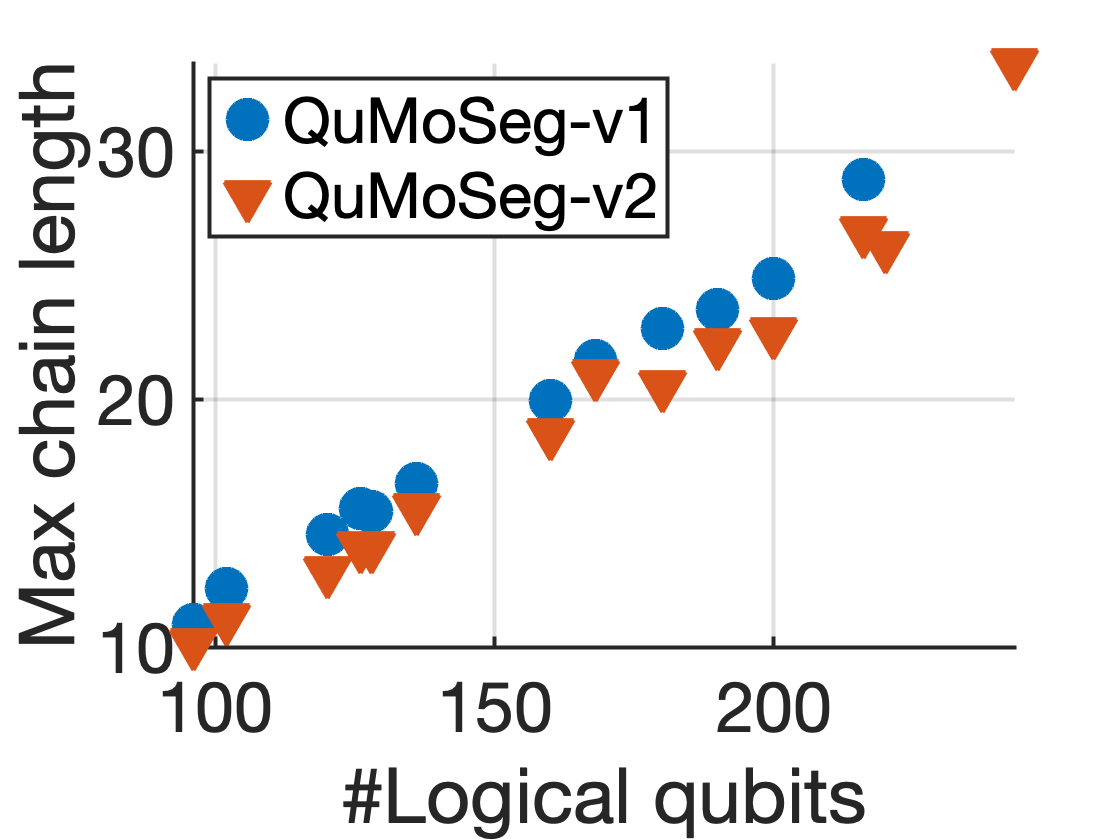
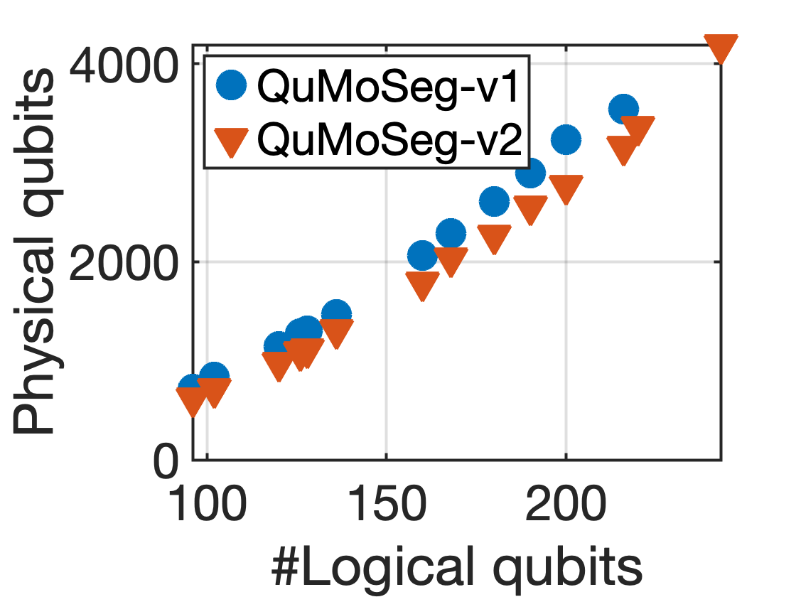
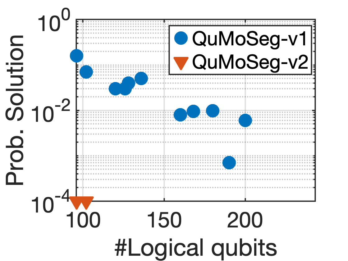
(b) Average maximum chain length (left), average number of physical qubits (middle) and probability of finding a solution (right) versus number of logical qubits in Q-MSEG dataset.

Figure 3: Results of synthetic experiments (a) and of real experiments on Q-MSEG (b).

Experiment with Synthetic Noise. We consider 20 synthetic configurations with 3 or 4 images, 2 motions and 16 points per image, resulting in 96 or 128 qubits. In order to create the ground-truth segmentation $X$, each point is assigned to a motion which is randomly chosen among the two available ones. All the analyzed methods can solve these problems with accuracy $\mu=1$. Next, we derive pairwise segmentations from (3) and we systematically inject into them increasing amounts of noise: in each pairwise segmentation we switch the motion of a percentage of points ranging from $0\%$ to $50\%$ (meaning that half of the points are corrupted). The results of this experiment are shown in Fig. 3a, which reports the accuracy (averaged over 20 problem instances) for the analyzed methods. QuMoSeg-v1 is certainly on par with the best traditional approach (namely Mode [4]). Concerning QuMoSeg-v2, it is worth noting that is starts from a similar formulation to Synch [4], but it solves the problem without relaxation: working over binary variables without relaxation in combination with AQC significantly improves the results. There are no significative differences between the two variants of our method on the smallest scenario with 96 qubits.

Experiments on Q-MSEG Dataset. Due to the lack of small-scale datasets usable for our scenario (i.e., whose size is manageable by current AQC), we generate a new dataset for motion segmentation with ground-truth annotations, which comprises six images depicting three planar objects captured from diverse viewpoints. We focus on planar motions (where the underlying model is the homography) since they can be recovered from a lower amount of points than general motions (where the corresponding model is the fundamental matrix), hence allowing more flexibility in the experimental setting. Each object is manually annotated with respectively 10, 11 and 12 keypoints, selected on highly-textured locations. Following [10, 61], we extract features corresponding to each keypoint using an AlexNet model [33] pretrained on ImageNet. Several motion segmentation problems are derived from the dataset: we consider 14 different choices for the number of points/images/motions (see supplementary), and we sample 20 problem instances for each configuration, resulting in 280 problem instances in total. For each problem instance, we perform feature matching on every image pair via nearest neighbor search, where the cosine distance is used as the distance metric. Then, different motions are identified in each image pair by fitting multiple homographies to correspondences [40]. This defines a set of pairwise segmentations which represent the input of Mode [5], Synch [4] and our quantum methods. In order to enrich the evaluation, we evaluate here also the method by Xu et al. [63] (with public code [1]), although it makes different assumptions on the input (i.e., it requires multi-frame trajectories, which were computed by us following the same procedure as in [5, 4]). For completeness, we also optimize the objective functions of our approach with a simulated annealing (SA) solver [32, 19]: while in general it performs on par with QA for smaller problems, it provides an indication on the QPU’s solution accuracy for the largest problems we test, which future QPU generations can potentially reach and outperform.

Table 1: Average accuracy (1 is the best) for several methods on our Q-MSEG dataset. The highest accuracy is in boldface.

# Qubits:	96	102	120	126	128	136	160	168	180	190	200	216	220	243
Xu et al. [63]	0.89	0.89	0.94	0.75	0.96	0.97	0.86	0.86	0.97	0.88	0.96	0.77	0.83	0.74
Mode [5]	0.93	0.93	0.96	0.93	0.97	0.97	0.98	0.99	0.98	0.99	0.99	0.93	1	0.94
Synch [4]	0.93	0.94	0.95	0.95	0.84	0.92	0.97	1	0.89	0.95	0.90	0.94	0.99	0.92
QuMoSeg-v1	0.97	0.97	0.97	0.96	0.95	0.98	0.98	0.99	0.98	0.99	0.99	0.64	–	–
QuMoSeg-v2	0.96	0.97	0.95	0.94	0.89	0.89	0.88	0.85	0.74	0.75	0.79	0.59	0.75	0.58
QuMoSeg-v1, SA	0.97	0.97	0.97	0.96	0.95	0.98	0.98	1	0.98	0.99	0.99	0.68	0.98	0.72
QuMoSeg-v2, SA	0.98	0.99	0.99	1	0.96	0.98	0.98	1	0.94	0.97	0.99	0.80	1	0.59

Results are given in Tab. 1 which reports, for each configuration, the mean accuracy $\mu$ (over 20 problem instances) for all the analyzed methods. Results show that there is no clear winner, since none of the methods outperforms all others in all cases. In particular, QuMoSeg-v1 is better than the state of the art on small-scale problems (i.e., 96-126 qubits) and comparable or better than the best traditional method (i.e., Mode [5]) on medium-scale problems (i.e., 136-200 qubits). On the largest cases, instead, either the performances of QuMoSeg-v1 significantly drop (i.e., 216 qubits) or it was unable to find a minor embedding and, hence, a solution (i.e., 220-243 qubits). Concerning QuMoSeg-v2, we can observe that—although working under easier assumptions—it is, in general, worse than QuMoSeg-v1. This might be caused by the difficulty of satisfying the additional (simplified) constraints in practice (as they are treated as soft instead of hard). Note that the performances of our approaches are largely affected by the limitation of current QPU. In this respect, the on-par or higher performance of SA (see Tab. 1) suggests that our QUBO approach to motion segmentation is sound and that future QPU generations are expected to reach or surpass that result. Qualitative results from an example with $96$ qubits are shown in Fig. 1: in this case, QuMoSeg-v1 outperforms existing methods.

Fig. 3b visualises how the expected number of physical qubits and the maximum chain length are increasing with the increasing problem size. It also reports the probability of finding a solution in a sampling, which is calculated as the portion of optimal (lowest-energy) solutions among all solutions. Note that QuMoSeg-v1 has a non-zero probability to find an optimal solution for all problems except the largest embeddable one with $216$ qubits, whereas QuMoSeg-v2 has a non-zero probability only on the two smallest cases.

Table 2: Accuracy ($1.0$ is the best) for several methods on sub-problems sampled from the Hopkins dataset [60]. The highest accuracy is in boldface.

# Qubits:	120	126	132	138	144	156	162	168	174	180	186	192	198	204	210	216	222	228	234	240
Xu et al. [63]	0.80	0.78	0.81	0.79	0.83	0.81	0.84	0.81	0.85	0.89	0.88	0.94	0.96	0.96	0.97	1	0.98	1	0.99	1
Mode [5]	0.89	0.91	0.90	0.93	0.92	0.94	0.95	0.95	0.96	0.95	0.97	0.98	0.98	0.98	0.98	0.99	0.98	0.98	0.99	0.99
Synch [4]	0.87	0.93	0.95	0.96	0.99	0.96	0.99	0.99	0.96	0.99	1	1	0.99	1	1	0.70	0.97	1	0.99	0.65
QuMoSeg-v1	0.92	0.89	0.93	0.93	0.93	0.93	0.95	0.94	0.96	0.95	0.96	0.97	0.96	-	-	-	-	-	-	-
QuMoSeg-v2	0.91	0.92	0.91	0.92	0.94	0.89	0.91	0.89	0.90	0.88	0.88	0.89	0.88	0.89	0.88	-	-	-	-	-
QuMoSeg-v1, SA	0.93	0.90	0.92	0.94	0.93	0.94	0.95	0.96	0.96	0.96	0.98	0.98	0.98	0.98	0.99	0.99	0.98	0.98	0.99	0.99
QuMoSeg-v2, SA	0.96	0.97	0.98	0.98	0.99	0.99	0.99	0.97	0.99	1	1	1	1	1	1	1	0.99	1	0.99	1

Experiments on Hopkins Benchmark. Starting from the popular Hopkins155 dataset [60], we created small problems (with 120-240 qubits) by sampling a subset of images/points from the cars2$\_$06$\_$g23 sequence (see our supplement for details). For each configuration, 20 instances were created, resulting in 400 examples in total. We used the fundamental matrix model to produce the pairwise segmentations which are given as input to Mode [5], Synch [4] and our quantum methods. We also consider the method by Xu et al. [63] and the simulated annealing (SA) solver [32, 19], as done previously. Results are given in Tab. 2, showing that we outperform Xu et al. [63] (for number of qubits ${<}198$) and obtain comparable performance to classic methods [5, 4] in several cases. Results for SA show that the global optima of our QUBOs match expected solutions (and that the obtained energy landscapes are as expected), even though the solutions cannot be recovered by QA in all cases due to hardware limitations. In particular, for small problems, the simulated annealing performs on par with QA (as expected), whereas large problems can be solved with the SA only.

Parameters. In the tests with Q-MSEG and Hopkins, we use $\lambda_{1}=10.0$ (v1) and $\lambda_{2}=10.0$, $\lambda_{3}=4.0$ (v2). For the synthetic experiments, we set the parameters as follows: $\lambda_{1}=14.0$ (v1) and $\lambda_{2}=27.5$, $\lambda_{3}=3.2$ (v2). The chain strength required to keep the chains of physical qubits intact, is chosen as a linear function $c(k)=ak+b$ in the number of the logical qubits. We set $a=0.13508$, $b=-1.94207$ and $a=0.1238$, $b=-1.3180$ for v1 and v2, respectively.

Discussion. In our experiments, QuMoSeg achieves on-par performance with non-quantum state of the art, showing the viability of a quantum approach for segmentation. Among the two proposed variants, QuMoSeg-v1 is the most accurate and QuMoSeg-v2 can solve larger problems. Moreover, our approach in a combination with SA shows highly promising results on both Q-MSEG and the data we generated from Hopkins. The characteristics of the current quantum hardware starkly influence the performance of QuMoSeg: Problems with ${>}120$ points cannot be minor-embedded, and the largest mappable problems require maintaining too long qubit chains, which impedes the optimum search. As many other quantum algorithms, QuMoSeg will benefit from improved quantum hardware, both in terms of accuracy and solvable problem sizes. Indeed, it is expected that the possibility to solve combinatorial problems without approximation will give practical advantages for large-scale problems in the future.

6 Conclusion

We propose the first motion segmentation approach for an adiabatic quantum computer, which shows highly promising results and reaches state-of-the-art accuracy on a wide range of problems. We hope that the demonstrated progress encourages more work on quantum computer vision in the future.

Appendix A Supplementary Material

This appendix provides further details on our experiments.

Competing methods. Mode [5], Synch [4] and Xu et al. [63] are evaluated in Matlab on a 2020 MacBook Pro with 1.4 GHz processor and 8 GB RAM.

Q-MSEG Dataset. We generate a new dataset for motion segmentation with ground-truth annotations, which comprises six images depicting three planar objects captured from diverse viewpoints, shown in Fig. 4. Each object is manually annotated with respectively 10, 11 and 12 keypoints, selected on highly-textured locations. Several motion segmentation problems are derived from the dataset by randomly sampling a subset of points/images/motions. In particular, we consider 14 different choices for the number of points/images/motions (see Table 3), and we sample 20 problem instances for each configuration, resulting in 280 problem instances in total. See Tab. 4 and the main paper for results.

Table 3: Statistics of the Q-MSEG Dataset. Each configuration has $n$ images and $d$ motions. In each image, there are $m_{1}$ points in the first motion, $m_{2}$ in the second motion and $m_{3}$ in the third motion (if available). The total number of logical qubits is reported for each configuration, which is given by $dn(m_{1}+m_{2}+m_{3})$.

# Qubits:	96	102	120	126	128	136	160	168	180	190	200	216	220	243
$n$	3	3	3	3	4	4	4	4	5	5	5	3	5	3
$d$	2	2	2	2	2	2	2	2	2	2	2	3	2	3
$m_{1}$	8	8	10	10	8	8	10	10	9	9	10	8	11	8
$m_{2}$	8	9	10	11	8	9	10	11	9	10	10	8	11	9
$m_{3}$	–	–	–	–	–	–	–	–	–	–	–	8	–	10

Figure 4: Images from the Q-MSEG dataset depicting three planar motions.

Parameter Selection. To select parameters for our method, we perform a systematic (exhaustive) grid search on small problem instances (with 24 bits). Talking in terms of the energy landscape, the purpose of this step is to find ranges of $\lambda$ which push the lowest-energy solution of the target QUBO as close as possible to the desired ground-truth solution. We observe that the obtained parameter ranges generalise well to larger problems when solved on a QPU (i.e., all tested problem sizes ranging from $96$ qubits to $243$ qubits). A similar observation was made in QSync [10]. Note that parameters can be selected in comparably large ranges, which allows safely using the same parameters across many—and much larger—problems. In particular, the parameters selected for our Q-MSEG dataset generalize well to Hopkins data without any tuning. Concerning the chain strength, the coefficients $a$ and $b$ of function $c$ (see the main paper) are calculated by a linear regression applied to the measured average maximum chain lengths observed in exemplary problems of different sizes (see Fig. 5).

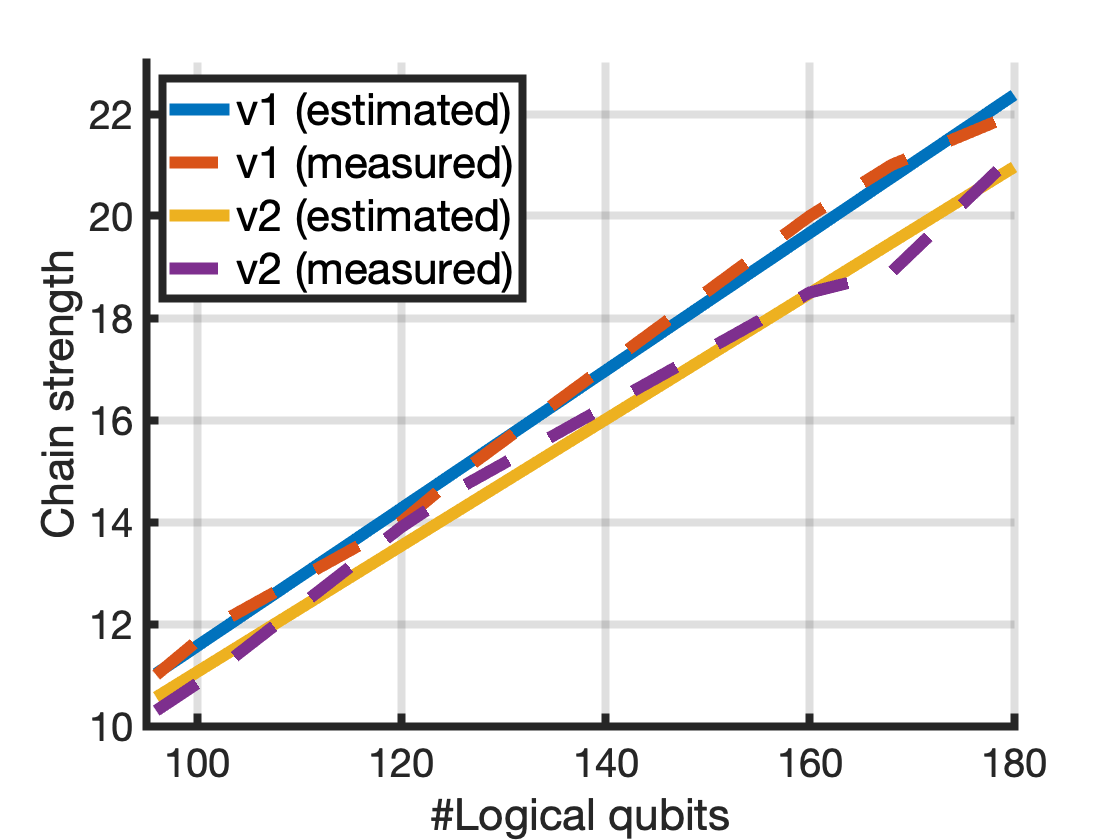
Figure 5: Chain strength versus number of logical qubits in Q-MSEG dataset.

Table 4: The accuracy ($1.0$ is the best) and its st. dev. for several methods on Q-MSEG dataset. For QuMoSeg, we also report the number of found ground-truth solutions (“$\#$sol”) and the probability (“prob”) of measuring them as lowest-energy samples, and we perform evaluation both on Adv1.1 and Adv4.1.

# Qubits:		96	102	120	126	128	136	160	168	180	190	200	216	220	243
Mode [5]	acc	0.93	0.93	0.96	0.93	0.97	0.97	0.98	0.99	0.98	0.99	0.99	0.93	1	0.94
	std	0.07	0.06	0.05	0.06	0.04	0.05	0.02	0.01	0.02	0.007	0.01	0.04	0	0.04
Synch [4]	acc	0.93	0.94	0.95	0.95	0.84	0.92	0.97	1	0.89	0.95	0.90	0.94	0.99	0.92
	std	0.14	0.15	0.08	0.14	0.21	0.15	0.03	0	0.15	0.15	0.20	0.06	0.003	0.11
Xu et al. [63]	acc	0.89	0.89	0.94	0.75	0.96	0.97	0.86	0.86	0.97	0.88	0.96	0.77	0.83	0.74
	std	0.18	0.12	0.08	0.14	0.05	0.04	0.18	0.16	0.04	0.10	0.06	0.09	0.15	0.05
	acc	0.97	0.97	0.97	0.96	0.95	0.98	0.98	0.99	0.98	0.99	0.99	0.64	–	–
QuMoSeg-v1	std	0.04	0.03	0.03	0.05	0.11	0.03	0.02	0.02	0.02	0.01	0.01	0.10	–	–
( Adv4.1 )	$\#$sol	9	5	6	11	6	11	8	9	7	6	9	0	–	–
	prob	0.16	0.07	0.03	0.03	0.04	0.05	0.008	0.0095	0.0097	0.0007	0.006	0	–	–
	acc	0.96	0.97	0.95	0.94	0.89	0.89	0.88	0.85	0.74	0.75	0.79	0.59	0.75	0.58
QuMoSeg-v2	std	0.03	0.02	0.03	0.02	0.09	0.04	0.03	0.10	0.12	0.07	0.04	0.10	0.06	0.07
( Adv4.1 )	$\#$sol	2	2	0	0	0	0	0	0	0	0	0	0	0	0
	prob	0.0001	0.0001	0	0	0	0	0	0	0	0	0	0	0	0
	acc	0.97	0.97	0.97	0.96	0.94	0.97	0.97	0.97	0.97	–	–	–	–	–
QuMoSeg-v1	std	0.04	0.02	0.03	0.05	0.11	0.04	0.03	0.03	0.03	–	–	–	–	–
( Adv1.1 )	$\#$sol	9	5	6	11	6	9	5	3	5	–	–	–	–	–
	prob	0.13	0.05	0.03	0.01	0.03	0.02	0.0003	0.0002	0.0007	–	–	–	–	–
	acc	0.95	0.96	0.93	0.92	0.86	0.86	0.97	0.81	0.69	0.67	0.71	0.59	0.66	–
QuMoSeg-v2	std	0.05	0.02	0.03	0.03	0.09	0.06	0.03	0.07	0.07	0.08	0.05	0.08	0.05	–
( Adv1.1 )	$\#$sol	1	0	0	0	0	0	5	0	0	0	0	0	0	–
	prob	0.0001	0	0	0	0	0	0.0003	0	0	0	0	0	0	–

Evaluation on Adv1.1. Table 4 reports our evaluation on D-Wave Advantage1.1 (Adv1.1). For reference, we also report results on Adv4.1 and those of competing methods, which are copied from the main paper. Results show that the accuracy on Adv1.1 is slightly lower than on Adv4.1, and the latter can solve larger problems. This is also reflected in the number of found ground-truth solutions and the probability of finding a ground-truth solution. Moreover, larger problems can be minor-embedded to Adv4.1 compared to Adv1.1. We also observe that for small problems, the accuracy of our method on Adv1.1 and Adv4.1 is similar, whereas for larger problems, Adv4.1 performs consistently better. This observation agrees with the statement done in Appendix A.1 Performance on Native Inputs of the technical report by McGeoch and Farré [42].

Hopkins Dataset. Starting from the well-known Hopkins155 dataset [60], we create small problems (with 120-240 qubits) by sampling a subset of images/points from the cars2$\_$06$\_$g23 sequence, which represents two moving objects in an outdoor environment. See Tab. 5 for the details. For each configuration, 20 instances were created, resulting in 400 examples in total. See the main paper for results on this dataset.

Table 5: Statistics of sub-problems sampled from the Hopkins dataset [60]. Each configuration has 3 images and 2 motions. In each image, there are $m_{1}$ points in the first motion and $m_{2}$ in the second motion. The total number of logical qubits is reported for each configuration, which is given by $6(m_{1}+m_{2})$.

# Qubits:	120	126	132	138	144	156	162	168	174	180	186	192	198	204	210	216	222	228	234	240
$m_{1}$	10	10	11	11	12	13	13	14	14	15	15	16	16	17	17	18	18	19	19	20
$m_{2}$	10	11	11	12	12	13	14	14	15	15	16	16	17	17	18	18	19	19	20	20

Minor Embeddings. Fig. 6 shows an exemplary minor embedding for a problem with $96$ qubits. Fig. 6-(left) is a photograph of the Adv4.1 processor. Fig. 6-(middle) and -(right) show the qubits graph of the logical problem ($96$ nodes) and its embedding into the processor ($803$ nodes), respectively. Each node in the logical problem graph is colored according to whether the qubit was measured as one (yellow) or zero (white). The figure on the right shows a section of the processor centered around the region with active qubits. The colors denote qubits measured—according to the Ising model—as ${+}1$ (blue) or ${-}1$ (white).

Figure 6: D-Wave Adv4.1 quantum annealer (left; reproduced with permission of D-Wave Systems), graph of $96$ logical problem qubits (middle) and its minor embedding with $803$ physical nodes (right).

References

- [1] https://alex-xun-xu.github.io/ProjectPage/CVPR_18/
- [2] https://github.com/federica-arrigoni/ICCV_19
- [3] Arrigoni, F., Fusiello, A.: Synchronization problems in computer vision with closed-form solutions. International Journal of Computer Vision 128, 26–52 (2020)
- [4] Arrigoni, F., Pajdla, T.: Motion segmentation via synchronization. In: IEEE International Conference on Computer Vision Workshops (ICCVW) (2019)
- [5] Arrigoni, F., Pajdla, T.: Robust motion segmentation from pairwise matches. In: Proceedings of the International Conference on Computer Vision (2019)
- [6] Barath, D., Matas, J.: Multi-class model fitting by energy minimization and mode-seeking. In: Proceedings of the European Conference on Computer Vision. pp. 229–245. Springer International Publishing (2018)
- [7] Bernard, F., Thunberg, J., Gemmar, P., Hertel, F., Husch, A., Goncalves, J.: A solution for multi-alignment by transformation synchronisation. In: Proceedings of the IEEE Conference on Computer Vision and Pattern Recognition (2015)
- [8] Bernard, F., Thunberg, J., Swoboda, P., Theobalt, C.: HiPPI: Higher-order projected power iterations for scalable multi-matching. In: Proceedings of the International Conference on Computer Vision (2019)
- [9] Birdal, T., Arbel, M., Simsekli, U., Guibas, L.J.: Synchronizing probability measures on rotations via optimal transport. In: Proceedings of the IEEE Conference on Computer Vision and Pattern Recognition. pp. 1566–1576 (2020)
- [10] Birdal, T., Golyanik, V., Theobalt, C., Guibas, L.: Quantum permutation synchronization. In: Proceedings of the IEEE Conference on Computer Vision and Pattern Recognition (2021)
- [11] Boothby, K., Bunyk, P., Raymond, J., Roy, A.: Next-Generation Topology of D-Wave Quantum Processors. arXiv e-prints 2003.00133 (2020)
- [12] Born, M., Fock, V.: Beweis des adiabatensatzes. Zeitschrift für Physik 51(3), 165–180 (1928)
- [13] Cai, J., Macready, W.G., Roy, A.: A practical heuristic for finding graph minors. arXiv e-prints 1406.2741 (2014)
- [14] Carlone, L., Tron, R., Daniilidis, K., Dellaert, F.: Initialization techniques for 3D SLAM: A survey on rotation estimation and its use in pose graph optimization. In: Proceedings of the IEEE International Conference on Robotics and Automation (2015)
- [15] Cavallaro, G., Willsch, D., Willsch, M., Michielsen, K., Riedel, M.: Approaching remote sensing image classification with ensembles of support vector machines on the d-wave quantum annealer. In: IEEE International Geoscience and Remote Sensing Symposium (IGARSS) (2020)
- [16] Chatterjee, A., Govindu, V.M.: Efficient and robust large-scale rotation averaging. In: Proceedings of the International Conference on Computer Vision (2013)
- [17] Chen, Y., Guibas, L., Huang, Q.: Near-optimal joint object matching via convex relaxation. In: Proceedings of the International Conference on Machine Learning. pp. 100–108 (2014)
- [18] D-Wave Systems, Inc.: D-wave ocean software documentation. https://docs.ocean.dwavesys.com/en/stable/ (2021), online; accessed on the 05.03.2022
- [19] D-Wave Systems, Inc.: dwave-neal documentation. https://docs.ocean.dwavesys.com/_/downloads/neal/en/latest/pdf/ (2021), online; accessed on the 6.03.2022
- [20] Dattani, N., Szalay, S., Chancellor, N.: Pegasus: The second connectivity graph for large-scale quantum annealing hardware. arXiv e-prints (2019)
- [21] Denchev, V.S., Boixo, S., Isakov, S.V., Ding, N., Babbush, R., Smelyanskiy, V., Martinis, J., Neven, H.: What is the computational value of finite-range tunneling? Phys. Rev. X 6, 031015 (2016)
- [22] D-wave: What is quantum annealing? https://docs.dwavesys.com/docs/latest/c_gs_2.html (2021), online; accessed on the 5.03.2022
- [23] Eriksson, A., Olsson, C., Kahl, F., Chin, T.J.: Rotation averaging and strong duality. In: Proceedings of the IEEE Conference on Computer Vision and Pattern Recognition. pp. 127–135 (2018)
- [24] Farhi, E., Goldstone, J., Gutmann, S., Lapan, J., Lundgren, A., Preda, D.: A quantum adiabatic evolution algorithm applied to random instances of an np-complete problem. Science 292(5516), 472–475 (2001)
- [25] Golyanik, V., Theobalt, C.: A quantum computational approach to correspondence problems on point sets. In: Proceedings of the IEEE Conference on Computer Vision and Pattern Recognition (2020)
- [26] Govindu, V.M., Pooja, A.: On averaging multiview relations for 3D scan registration. IEEE Transactions on Image Processing 23(3), 1289–1302 (2014)
- [27] Grant, E.K., Humble, T.S.: Adiabatic quantum computing and quantum annealing. In: Oxford Research Encyclopedia of Physics (2020)
- [28] Hartley, R., Zisserman, A.: Multiple View Geometry in Computer Vision. Cambridge University Press, second edn. (2004)
- [29] Huang, J., Wang, H., Birdal, T., Sung, M., Arrigoni, F., Hu, S.M., Guibas, L.J.: Multibodysync: Multi-body segmentation and motion estimation via 3d scan synchronization. In: Proceedings of the IEEE Conference on Computer Vision and Pattern Recognition. pp. 7108–7118 (2021)
- [30] Ji, P., Li, H., Salzmann, M., Dai, Y.: Robust motion segmentation with unknown correspondences. In: Proceedings of the European Conference on Computer Vision. pp. 204–219. Springer International Publishing (2014)
- [31] Ji, P., Salzmann, M., Li, H.: Shape interaction matrix revisited and robustified: Efficient subspace clustering with corrupted and incomplete data. In: Proceedings of the International Conference on Computer Vision. pp. 4687–4695 (2015)
- [32] Kirkpatrick, S., Gelatt, C.D., Vecchi, M.P.: Optimization by simulated annealing. Science 220(4598), 671–680 (1983)
- [33] Krizhevsky, A., Sutskever, I., Hinton, G.E.: Imagenet classification with deep convolutional neural networks. In: Advances in Neural Information Processing Systems. vol. 25 (2012)
- [34] Lai, T., Wang, H., Yan, Y., Chin, T.J., Zhao, W.L.: Motion segmentation via a sparsity constraint. IEEE Transactions on Intelligent Transportation Systems 18(4), 973–983 (2017)
- [35] Li, J., Ghosh, S.: Quantum-soft qubo suppression for accurate object detection. In: European Conference on Computer Vision (ECCV) (2020)
- [36] Li, X., Ling, H.: Pogo-net: Pose graph optimization with graph neural networks. In: Proceedings of the International Conference on Computer Vision. pp. 5895–5905 (2021)
- [37] Li, Z., Guo, J., Cheong, L.F., Zhou, S.Z.: Perspective motion segmentation via collaborative clustering. In: Proceedings of the International Conference on Computer Vision. pp. 1369–1376 (2013)
- [38] Liu, S., Trenkler, G.: Hadamard, Khatri-Rao, Kronecker and other matrix products. International Journal of Information and Systems Sciences 4(1), 160 – 177 (2008)
- [39] Magri, L., Fusiello, A.: T-Linkage: A continuous relaxation of J-Linkage for multi-model fitting. In: Proceedings of the IEEE Conference on Computer Vision and Pattern Recognition. pp. 3954–3961 (June 2014)
- [40] Magri, L., Fusiello, A.: Robust multiple model fitting with preference analysis and low-rank approximation. In: Proceedings of the British Machine Vision Conference. pp. 20.1–20.12. BMVA Press (September 2015)
- [41] Maset, E., Arrigoni, F., Fusiello, A.: Practical and efficient multi-view matching. In: Proceedings of IEEE International Conference on Computer Vision. pp. 4568–4576 (2017)
- [42] McGeoch, C., Farré, P.: The advantage system: Performance update (2021-10-01). https://www.dwavesys.com/media/qdmlgsu1/14-1054a-a_advantage_system_performance_update.pdf (2021), online; accessed on the 20.02.2022
- [43] McGeoch, C.C.: Adiabatic Quantum Computation and Quantum Annealing: Theory and Practice. Morgan & Claypool (2014)
- [44] Noormandipour, M., Wang, H.: Matching Point Sets with Quantum Circuit Learning. arXiv e-prints 2102.06697 (2021)
- [45] Ozden, K.E., Schindler, K., Van Gool, L.: Multibody structure-from-motion in practice. IEEE Transactions on Pattern Analysis and Machine Intelligence 32(6), 1134–1141 (2010)
- [46] Ozyesil, O., Voroninski, V., Basri, R., Singer, A.: A survey of structure from motion. Acta Numerica 26, 305 – 364 (2017)
- [47] O’Malley, D., Vesselinov, V.V., Alexandrov, B.S., Alexandrov, L.B.: Nonnegative/binary matrix factorization with a d-wave quantum annealer. PLOS ONE 13(12) (12 2018)
- [48] Pachauri, D., Kondor, R., Singh, V.: Solving the multi-way matching problem by permutation synchronization. In: Advances in Neural Information Processing Systems, vol. 26, pp. 1860–1868 (2013)
- [49] Rao, S., Tron, R., Vidal, R., Ma, Y.: Motion segmentation in the presence of outlying, incomplete, or corrupted trajectories. Pattern Analysis and Machine Intelligence 32(10), 1832–1845 (2010)
- [50] Rosen, D.M., Carlone, L., Bandeira, A.S., Leonard, J.J.: Se-sync: A certifiably correct algorithm for synchronization over the special euclidean group. The International Journal of Robotics Research 38(2-3), 95–125 (2019)
- [51] Sabzevari, R., Scaramuzza, D.: Multi-body motion estimation from monocular vehicle-mounted cameras. IEEE Transactions on Robotics 32(3), 638–651 (2016)
- [52] Santellani, E., Maset, E., Fusiello, A.: Seamless image mosaicking via synchronization. ISPRS Annals of Photogrammetry, Remote Sensing and Spatial Information Sciences IV-2, 247–254 (2018)
- [53] Saputra, M.R.U., Markham, A., Trigoni, N.: Visual SLAM and structure from motion in dynamic environments: A survey. ACM Computing Surveys 51(2), 37:1–37:36 (2018)
- [54] Schroeder, P., Bartoli, A., Georgel, P., Navab, N.: Closed-form solutions to multiple-view homography estimation. In: IEEE Workshop on Applications of Computer Vision (WACV). pp. 650–657 (2011)
- [55] Seelbach Benkner, M., Golyanik, V., Theobalt, C., Moeller, M.: Adiabatic quantum graph matching with permutation matrix constraints. In: International Conference of 3D Vision (3DV) (2020)
- [56] Seelbach Benkner, M., Lähner, Z., Golyanik, V., Wunderlich, C., Theobalt, C., Moeller, M.: Q-match: Iterative shape matching via quantum annealing. In: International Conference on Computer Vision (ICCV) (2021)
- [57] Singer, A.: Angular synchronization by eigenvectors and semidefinite programming. Applied and Computational Harmonic Analysis 30(1), 20 – 36 (2011)
- [58] Thunberg, J., Bernard, F., Goncalves, J.: Distributed methods for synchronization of orthogonal matrices over graphs. Automatica 80, 243–252 (2017)
- [59] Tron, R., Danilidis, K.: Statistical pose averaging with varying and non-isotropic covariances. In: Proceedings of the European Conference on Computer Vision (2014)
- [60] Tron, R., Vidal, R.: A benchmark for the comparison of 3-d motion segmentation algorithms. In: Proceedings of the IEEE Conference on Computer Vision and Pattern Recognition. pp. 1–8. IEEE (2007)
- [61] Wang, Q., Zhou, X., Daniilidis, K.: Multi-image semantic matching by mining consistent features. Computer Vision and Pattern Recognition (CVPR) (2018)
- [62] Wang, Y., Liu, Y., Blasch, E., Ling, H.: Simultaneous trajectory association and clustering for motion segmentation. IEEE Signal Processing Letters 25(1), 145–149 (2018)
- [63] Xu, X., Cheong, L.F., Li, Z.: 3d rigid motion segmentation with mixed and unknown number of models. IEEE Transactions on Pattern Analysis and Machine Intelligence (2019)
- [64] Yan, J., Pollefeys, M.: A general framework for motion segmentation: Independent, articulated, rigid, non-rigid, degenerate and nondegenerate. In: Proceedings of the European Conference on Computer Vision. pp. 94–106 (2006)
- [65] Zhou, X., Zhu, M., Daniilidis, K.: Multi-image matching via fast alternating minimization. In: Proceedings of the International Conference on Computer Vision. pp. 4032 – 4040 (2015)