Kolmogorov Turbulence Coexists with Pseudo-Turbulence
in Buoyancy-Driven Bubbly Flows

Abstract

We investigate the spectral properties of buoyancy-driven bubbly flows. Using high-resolution numerical simulations and phenomenology of homogeneous turbulence, we identify the relevant energy transfer mechanisms. We find: (a) At a high enough Galilei number (ratio of the buoyancy to viscous forces) the velocity power spectrum shows the Kolmogorov scaling with a power-law exponent $-5/3$ for the range of scales between the bubble diameter and the dissipation scale ($\eta$). (b) For scales smaller than $\eta$, the physics of pseudo-turbulence is recovered.

The flow behind an array of cylinders or a grid, either moving or stationary, provides an ideal testbed to verify and scrutinize the statistical theories of turbulence [1]. What is the flow generated when a fluid is stirred by a dilute suspension of bubbles as they rise due to buoyancy? This question has intrigued researchers for the past three decades due to their occurrence in both industrial and natural processes [2, 3, 4, 5, 6, 7]. Experiments [8, 9, 10, 11, 12, 13] and numerical simulations [14, 15, 16] show that flows generated by dilute bubble suspensions are chaotic and originate due to the interplay of viscous, inertial, and surface tension forces. The complex spatio-temporal flow is called “pseudo-turbulence” or “bubble induced agitation” [3, 5].

As is typical for chaotic flows, pseudo-turbulence is characterized by the power spectrum of its velocity fluctuations $E(k)$, which shows a power law scaling $E(k)\sim k^{-\alpha}$ with an exponent $\alpha\gtrsim 3$ in the wavenumber range $k\gtrsim k_{\rm d}$ where $k_{\rm d}=2\pi/d$ and $d$ is the bubble diameter [8, 12]. Lance & Bataille [8] argued that the balance of energy production with viscous dissipation may explain the observed scaling. Recent numerical studies conducted for experimentally accessible Galilei numbers Ga (the ratio of buoyancy to viscous dissipation), show that the net production has contributions both from the advective nonlinearity and the surface tension [14, 15, 16, 11, 15].

In homogeneous and isotropic turbulence (HIT) the energy injected at an integral scale $\mathcal{L}$ is transferred to dissipation scale $\eta\ll\mathcal{L}$, via the advective interactions without dissipation while maintaining a constant energy flux. This intermediate range of scales between $\eta$ and $\mathcal{L}$ is called the inertial range. At scale smaller than $\eta$ the advective interactions balance viscous dissipation [17]. Clearly within the phenomenology of homogeneous and isotropic turbulence, pseudo-turbulence is a dissipation range phenomena with the additional complexity due to surface tension forces. Is it possible to have an inertial range in buoyancy driven bubbly flows?

In this paper, we present state-of-the-art direct numerical simulations of buoyancy driven bubbly flows, at high resolution, which allows us to access $\mbox{Ga}>1000$ which has never been achieved before in either experiments or numerical simulations. Our multiphase simulations model a dilute suspension of “gas” bubbles of lighter phase (density $\rho_{\rm 1}$) dispersed in the heavier “liquid” phase (density $\rho_{\rm 2}$). The density contrast is parametrised by the Atwood number, $\mbox{At}\equiv(\rho_{\rm 2}-\rho_{\rm 1})/(\rho_{\rm 2}+\rho_{\rm 1})$. We consider both small ($0.04$) and large ($0.8,0.98$) values for At. We use two different codes for these two cases. In both of these cases, we find, for the first time, a direct evidence for Kolmogorov scaling, $E(k)\sim k^{-5/3}$, for $k_{\rm d}\leq k\lesssim 1/\eta$. For scales smaller than $\eta$, the physics of pseudo-turbulence is recovered. By analyzing the scale-by-scale energy budget we uncover the mechanism by which the Kolmogorov scaling emerges: for high enough Ga, for both small and larger At, there is an intermediate range of scales over which the contribution from advection dominates over all other contributions (including surface tension) in the kinetic energy budget. This is the range over which Kolmogorov scaling is observed.

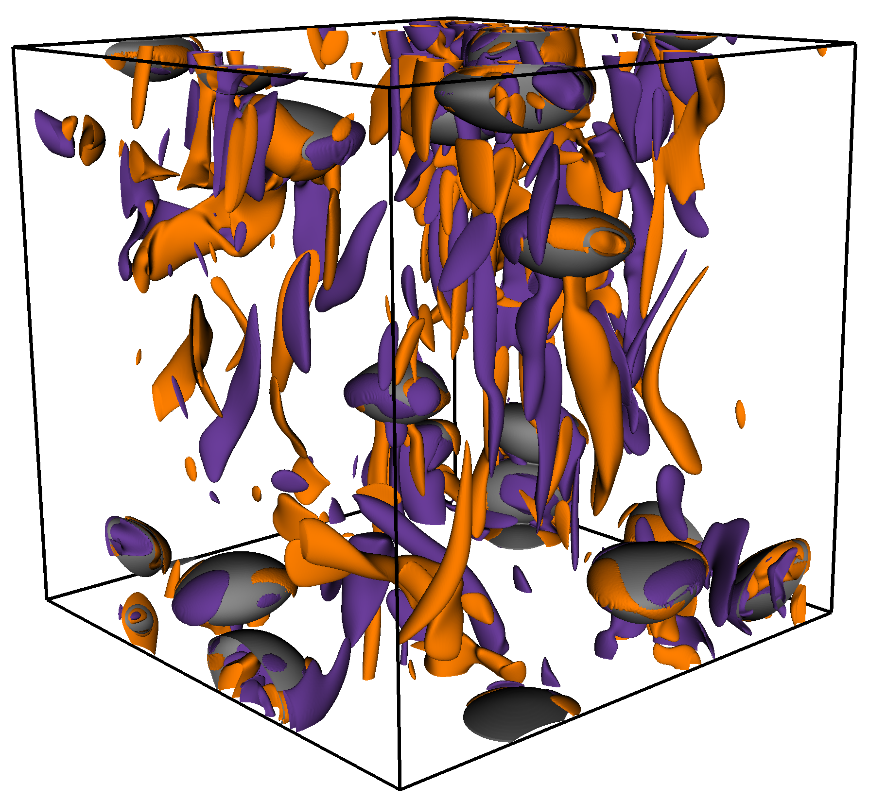
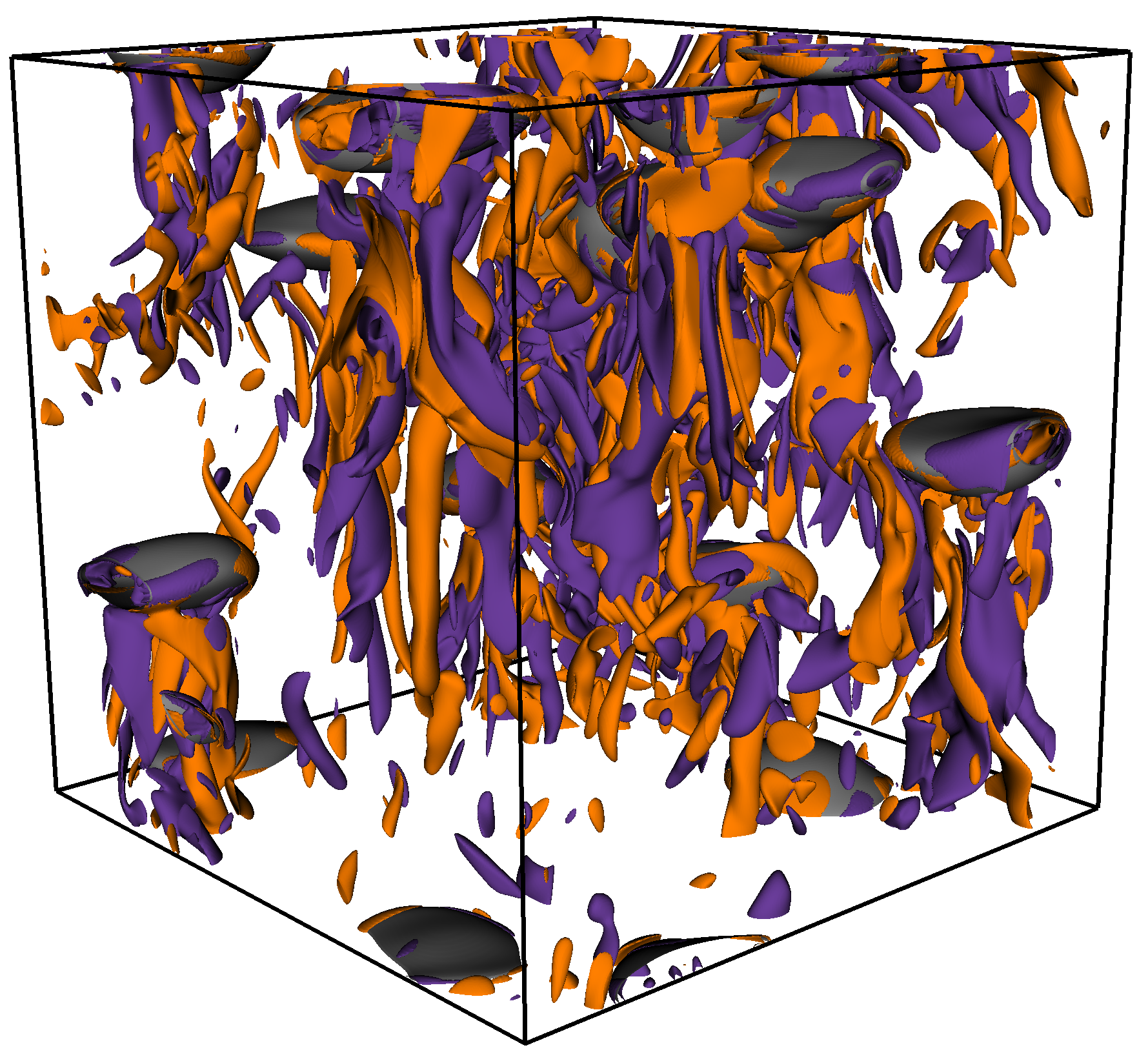
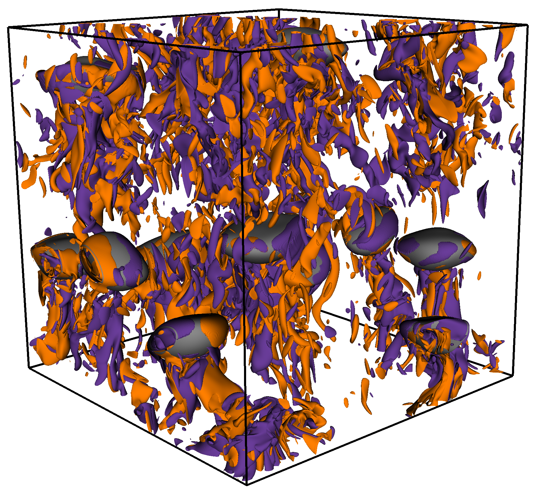
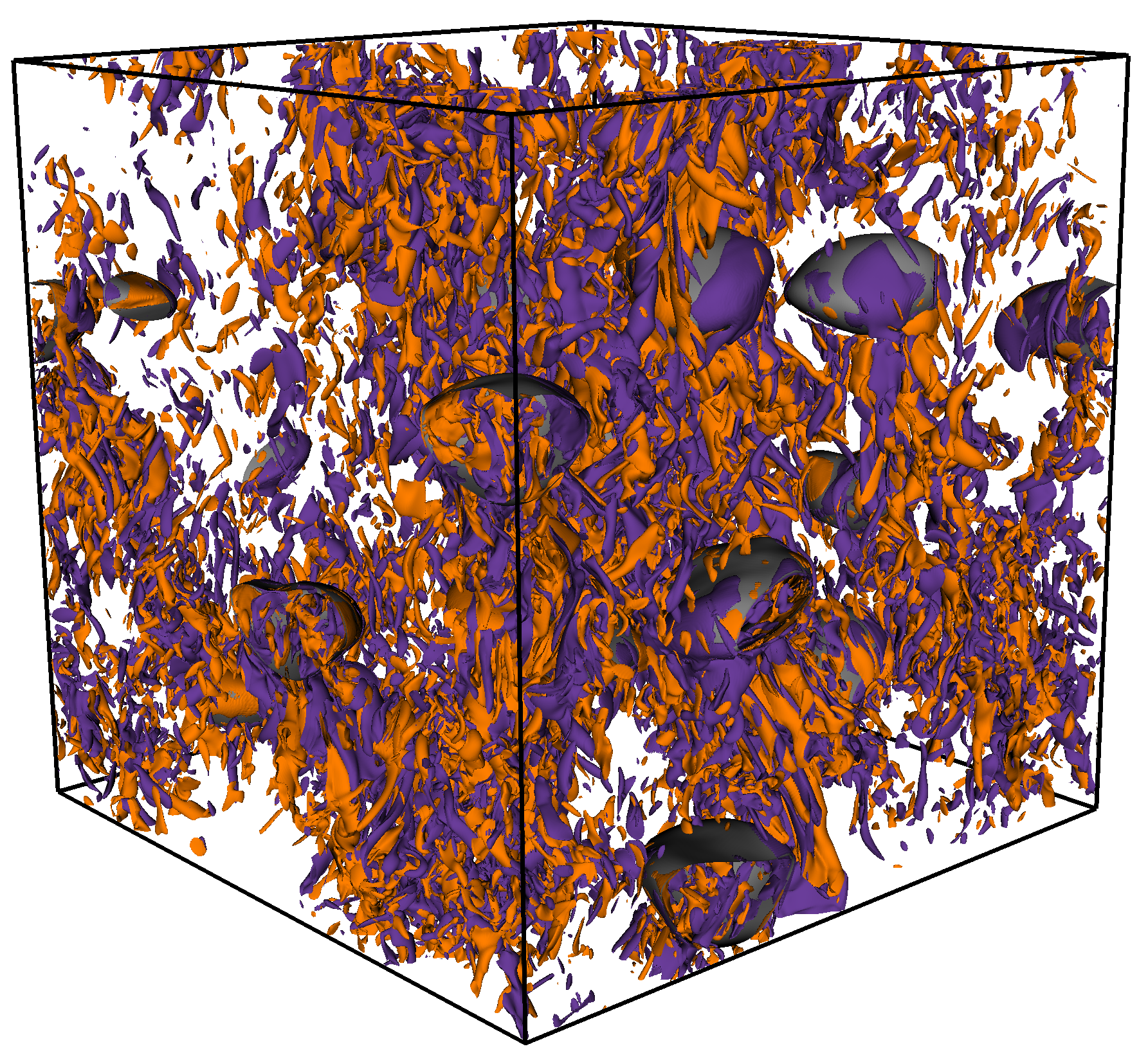
Figure 1: The iso-contour plot of the z-component of the vorticity $\omega^{z}=\left({\nabla}\times\bm{u}\right)\cdot\hat{\bm{z}}$ for (left to right) $\mbox{Ga}=302,~{}605,~{}1029$, and $2057$. We show the contour corresponding to $\pm\left\langle\left(\omega^{z}\right)^{2}\right\rangle^{1/2}$ in purple and orange respectively. The bubbles are represented using grey contours.

We study the dynamics of bubbly flow using multi-phase Navier-Stokes equations [14] for an incompressible velocity field ${\bm{u}}=(u^{x},u^{y},u^{z})$,

$$\rho(\partial_{t}\bm{u}+\bm{u}\cdot{\nabla}\bm{u}) =\mu\nabla^{2}\bm{u}-{\nabla}p+\bm{F}^{\rm\sigma}+\bm{F}^{\rm g}\/,~{}\text{where}$$ (1a)

$$\bm{F}^{\rm g}\equiv(\rho(c)-\rho_{\rm a}) {\bm{g}}=\mbox{At}(\rho_{\rm 2}+\rho_{\rm 1})(c-c_{\rm a}){\bm{g}}\/,~{}\text{and}$$ (1b)

$$\bm{F}^{\rm\sigma}\equiv\int\sigma\kappa\hat{\bm{n}}\delta(\bm{x} -\bm{x}_{\rm b})\mathop{{\rm d}s},$$ (1c)

where the bulk viscosity $\mu$ is assumed to be identical in both the phases, and $p$ is the pressure. An indicator function $c$, distinguishes the liquid ($c=1$) and the gas ($c=0$) phase [18, 19]. The density field $\rho(c)=\rho_{\rm 2}c+\rho_{\rm 1}(1-c)$. In Eq. (1), the buoyancy force is $\bm{F}^{\rm g}$, $c_{\rm a}\equiv(1/V)\int c{\rm d}V$ is the indicator function averaged over the volume $V$ of the simulation domain, $\rho_{\rm a}=\rho_{\rm 1}+(\rho_{\rm 2}-\rho_{\rm 1})c_{\rm a}$ is the average density,  ${\bm{g}}\equiv-g\hat{\bm{z}}$ is the acceleration due to gravity, and $\hat{\bm{z}}$ is the unit vector along the vertical (positive $z$) direction. The surface tension force is denoted by $\bm{F}^{\rm\sigma}$, where $\sigma$ is the coefficient of the surface tension, $\kappa$ is the local curvature of the bubble-front located at $\bm{x}_{\rm b}$, $\hat{\bm{n}}$ is the unit normal, and $\mathop{{\rm d}s}$ is the infinitesimal surface area of the bubble.

For the small $\mbox{At}=0.04$ case, we invoke Boussinesq approximation [20] wherein the density variations can be ignored $\rho\approx\rho_{\rm a}$, and the buoyancy force simplifies to $\bm{F}^{\rm g}=2\rho_{\rm a}\mbox{At}(c-c_{a})$ [14, 15]. We solve Eq. (1) numerically using the pseudo-spectral method [21] in a three-dimensional periodic domain where each side is of length $L$, discretized uniformly into $N$ collocation points. We numerically integrate the bubble phase using a front-tracking method [14, 22, 19]. For time-evolution, we use a second-order exponential time differencing scheme [23] for Eq. (1) and a second-order Runge-Kutta scheme to update the front. For the large $\mbox{At}=0.8,$ and $0.98$, we use the front tracking module of an open-source multiphase solver PARIS [24], where both spatial and temporal derivatives are approximated using a second-order central-difference scheme.

Consistent with the experiments designed to study buoyancy driven bubbly flows [12, 13, 8] we choose the volume fraction of the bubbles $\phi\leq 5\%$. At these volume fraction, the effects coalescence or breakup of the bubbles can be ignored [25]. The front-tracking scheme is ideally suited to study this parameter range because it ignores both coalescence and breakup. For one representative case we also perform Volume-of-Fluid (VoF) simulation (vof-R5) using PARIS – VoF simulations allow coagulation and break-up – to confirm that coalescence plays no significant role.

In what follows, the following non-dimensional numbers will be used: Atwood number At defined previously, the Galilei number $\mbox{Ga}\equiv\sqrt{(\rho_{2}-\rho_{1})gd^{3}/\rho_{2}\nu^{2}}$, the Bond number $\mbox{Bo}\equiv{(\rho_{2}-\rho_{1})gd^{2}/\sigma}$, the integral scale Reynolds number $\mbox{Re}_{\mathcal{L}}^{3/4}\equiv\mathcal{L}/\eta$, the Taylor-microscale Reynolds number $\mbox{Re}_{\lambda}\equiv u_{\rm rms}^{2}\sqrt{15\rho_{2}/(\nu\epsilon^{\rm g})}$. Here we have used, kinematic viscosity $\nu=\mu/\rho_{2}$, the large eddy turnover time $\tau_{L}\equiv{\cal L}/u_{\rm rms}$, the root-mean-square velocity, $u_{\rm rms}$, the energy injection rate by the buoyant forces , $\epsilon^{\rm g}\equiv(1/V)\int\bm{F}^{\rm g}\cdot\bm{u}\mathop{{\rm d}V}$, integral length scale ${\mathcal{L}}\equiv(3\pi/4)[\sum_{k}E(k)/k]/\sum_{k}E(k)$ and the Kolmogorov dissipation scale $\eta\equiv(\rho_{\rm a}\nu^{3}/\epsilon^{\rm g})^{1/4}$ The different parameters of our simulations are given in Table. (1).

runs	R1	R2	R3	R4	R5	R6	vof-R5	R7	${\tt R8}$	${\tt R9}$
$N$	$256$	$512$	$512$	$512$	$720$	$720$	$1024$	$288$	$504$	$504$
Ga	$103$	$302$	$403$	$605$	$1029$	$2057$	$1029$	$340$	$1059$	$1489$
At	$0.04$	$0.04$	$0.04$	$0.04$	$0.04$	$0.04$	$0.04$	$0.8$	$0.8$	$0.98$
$\mbox{Re}_{\lambda}$	$11.8$	$30.7$	$37.9$	$47.8$	$60.7$	$96.9$	$60.7$	$28.8$	$69.3$	$88.1$
${\mathcal{L}}/\eta$	$12.6$	$26.3$	$29.5$	$38.8$	$50.4$	$80$	$50.4$	$20.5$	$46$	$56.0$

Table 1: Parameters of simulations. The Bond number $\mbox{Bo}=1.75$, number of bubbles $N_{\rm b}=12$, the diameter of the bubble $d=1.08$, $L=2\pi$, $\rho_{2}=1.0$, and the volume fraction of the bubbles $\phi=3.2\%$ are same in all the runs. For all the runs ${\mathcal{L}}\sim d$, and the statistics are averaged over a period of at least $5\tau_{L}$ in the stationary state (see Supplementary material). Total energy injection rate $\epsilon^{\rm g}=0.031\pm 0.002$ in all the case.

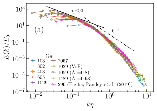
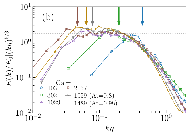
Figure 2: (a) Log-log plot of the normalized velocity power spectra $E(k)$ as a function of $k\eta$ for various Ga. We observe Kolmogorov scaling $E(k)\sim k^{-5/3}$ for $k\eta\lesssim 0.3$, and the pseudo-turbulence scaling $E(k)\sim k^{-3}$ for $k\eta\gtrsim 0.3$. (b) The velocity power spectra for different Ga compensated by $k^{5/3}$. In (b) the vertical arrows show the wavenumber corresponding to the bubble diameter $k_{\rm d}\eta$.

We start our simulation by placing $N_{\rm b}$ bubbles randomly in the domain. It takes around $4.5\tau_{L}$ for our simulation attain a statistically stationary state. Once it is reached, all our data are averaged over at least $5\tau_{L}$. In Fig. (1) we show the iso-contour plot of the $z$-component of vorticity $\omega^{z}=\left({\nabla}\times\bm{u}\right)\cdot\hat{\bm{z}}$. As the Ga ($\mbox{Re}_{\lambda}$) is increased, not only the intense vortical regions in the field increases, we observe flow structures at much smaller scales as well.

Next we investigate power spectrum of velocity fluctuations:

$$E(k)=\frac{1}{2}\sum_{\bm{k}}\left\langle\hat{\bm{u}}(\bm{k})\hat{\bm{u}}(-\bm{k})\right\rangle\delta(|\bm{k}|-k),$$ (2)

where $\hat{\bm{u}}(\bm{k})$ is the Fourier transform of the velocity field $\bm{u}$, $\bm{k}$ the wavevector and $\left\langle\cdot\right\rangle$ denotes spatiotemporal average over the statistically stationary state of turbulence. Kolmogorov theory of turbulence shows that, in homogeneous and isotropic turbulence, $E(k)$ for different Reynolds numbers collapses onto a single curve if we use $\eta$ as the characteristic length scale and $E_{\rm 0}=\left(\epsilon^{\rm g}\nu^{5}/\rho_{2}\right)^{1/4}$ as the characteristic energy scale, which we use henceforth. In Fig. (2a) we show that, even for buoyancy driven bubbly turbulence, the same data–collapse holds for scales $k\gtrsim k_{\rm d}$. For small Ga number we obtain the pseudo–turbulence regime [8, 12, 13, 14] for $k\gtrsim 0.3/\eta$. As the Ga increases an scaling range with an exponent of approximately $-5/3$ emerges for $k_{\rm d}\lesssim k\lesssim 0.3/\eta$. This is a novel, previously unobserved scaling in bubbly flows. The scaling range increases with Ga; it is almost non-existent for $\mbox{Ga}=100$ and extends up to almost half a decade for $\mbox{Ga}=2057$. The $-5/3$ scaling range is best seen in Fig. (2b) where we plot the spectra compensated with $k^{5/3}$. As we have used $\eta$ as our characteristic length scale the Fourier mode $k_{\rm d}$, shown by an arrow appears at different locations in this plot. As Ga is increased $k_{\rm d}$ moves to the left thereby the $-5/3$ scaling range emerges.

Note that due to rising bubbles, in principle, our flow is anisotropic. Here and henceforth, following the standard practice in bubbly turbulence [8, 14, 16], we use the isotropic spectra which is the projection of the general anisotropic spectra on to the isotropic sector [27]. In the supplementary material, which includes Ref. [27], we show that for our simulations the anisotropic contribution is negligible at all scales except $k$ in the neighbourhood of $k_{\rm d}$.

We now describe how Kolmogorov scaling emerges at both small and large At by studying the scale-by-scale energy budget equation:

$$\partial_{t}\mathcal{E}_{\rm K}=-\Pi_{K}-\mathscr{F}^{\sigma}_{K}+\mathscr{P}_{K}-\mathscr{D}_{K}+\mathscr{F}^{\rm g}_{K}\/.$$ (3)

Here $\mathcal{E}_{\rm K}$ is the kinetic energy contained up-to wavenumber $K$. Here $\Pi_{K}$, $\mathscr{F}^{\sigma}_{K}$, $\mathscr{P}_{K}$, $\mathscr{D}_{K}$ and $\mathscr{F}^{\rm g}_{K}$ are the contributions from the advective term, surface tension, pressure, viscous dissipation and buoyancy from Eq. (1) .

The scale-by-scale budget for low ${\mbox{At}=0.04}$ — we follow Refs. [29, 30, 17, 31] to derive Eq. (3). We consider stationary state, hence $\partial_{t}\mathcal{E}_{\rm K}=0$ and we use Boussinesq approximation, hence $\mathscr{P}_{K}=0$. We plot all the others terms of Eq. (3) as a function of $K$ in the top row of Fig. (3) for large and small Ga. As expected [14], bubbles inject energy into the flow at scales comparable to the bubble diameter – $\mathscr{F}^{\rm g}_{K}$ monotonically increases and saturates around $K\approx k_{\rm d}$. From the perspective of the Kolmogorov theory of turbulence [17, section 6.2.4] the buoyancy injection term $\mathscr{F}^{\rm g}_{K}$ is the large scale driving force active at scales around $k_{\rm d}$. Following Ref. [17], consider a fixed $K\gg k_{\rm d}$ and take the limit $\nu\to 0$ ($\mbox{Ga}\to\infty$). Then $\displaystyle\lim_{\nu\to 0}\mathscr{D}_{K}\approx 0$, holds and the flux balance equation reads:

$$\Pi_{K}+\mathscr{F}^{\sigma}_{K}=\epsilon^{\rm g}\/.$$ (4)

Because the injection is limited to Fourier modes around $k_{\rm d}$, for $K\gg k_{\rm d}$, $\mathscr{F}^{\rm g}_{K}\approx\epsilon^{\rm g}$ is a constant. In homogeneous and isotropic turbulence in absence of bubbles the dissipative effects become significant around $8$ to $10\eta$ [32]. We find $3\eta$ is a reasonable approximation in our case. Thus, Eq. (4) is expected to be valid for $k_{\rm d}<K\lesssim 0.3/\eta$ – this range is shaded with light blue in Fig. (3). Within the shaded region $\Pi_{K}\gg\mathscr{F}^{\sigma}_{K}$, hence $\Pi_{K}\approx\epsilon^{\rm g}/2$ is a constant leading to the Kolmogorov $-5/3$ scaling in the energy spectrum [17]. Even at $\mbox{Ga}=2057$, the $-5/3$ scaling range is at best close to a decade. In Fig. (3b), for $\mbox{Ga}=302$ the shaded region has practically disappeared. For this and other other runs with smaller Ga, we expect to observe pseudo-turbulence where none of the three fluxes, $\mathscr{F}^{\sigma}_{K}$, $\Pi_{K}$ and $\mathscr{D}_{K}$, can be ignored. A detailed discussion on the flux balance in the pseudo-turbulence regime for $\mbox{Ga}\leq 360$ can be found in our earlier studies [15, 14, 22].

The scale-by-scale budget for high ${\mbox{At}=0.8,0.98}$ — we follow Refs. [29, 33, 34] to derive Eq. (3). We again consider statistical stationarity, hence $\partial_{t}\mathcal{E}_{\rm K}=0$. In Fig. (3c-e), we plot all the terms of Eq. (3) as a function of $K$ for both high and low Ga. The “baropycnal work”, $\mathscr{P}_{K}$, now provide an alternate routes for nonlinear energy transfer. The baropycnal term has contributions from the barotropic generation of strain and baroclinic generation of vorticity due to density variations [34]. Remarkably, for large enough Ga there is a range of scales, shaded in Fig. (3c,e) where the dominant balance is $\Pi_{K}\approx\epsilon^{\rm g}/2$ is a constant leading to the Kolmogorov $-5/3$ scaling in the energy spectrum. The other transfer mechanisms $\mathscr{F}^{\sigma}_{K}$ and $\mathscr{P}_{K}$ are sub-dominant. A positive slope of $\mathscr{F}^{\sigma}_{K}$ ($\mathscr{P}_{K}$) indicates that the energy is absorbed (injected), whereas a negative slope indicates energy being injected (absorbed). Thus surface tension absorbs energy at large scales and injects it at small scales, whereas the opposite is the case for the baropycnal term.

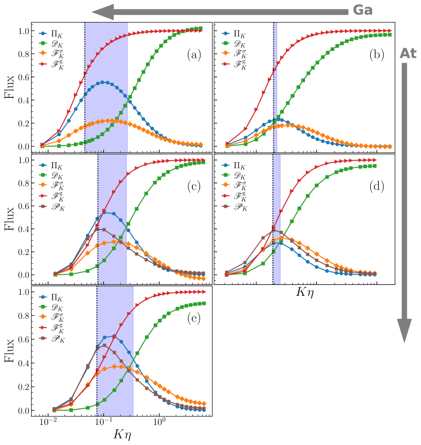
Figure 3: Semi-log plot of the different terms in scale-by-scale budget for low Atwood number $\mbox{At}=0.04$ (top row) with $\mbox{Ga}=2057$ (a) and $\mbox{Ga}=302$ (b); $\mbox{At}=0.8$ (middle row) for $\mbox{Ga}=1029$ (c), $\mbox{Ga}=345$ (d); and $\mbox{At}=0.98$ (bottom row), $\mbox{Ga}=1489$ (e). The abscissa is normalized by the total energy injection rate $\epsilon^{\rm g}$. The dashed vertical line represents the wave-number corresponding to bubble diameter, $k_{\rm d}$. The continuous vertical line shows the wavenumber where the advective flux and the dissipative flux crosses. The region between these two lines, where the advective contribution dominates, is shaded with light blue color.

Several earlier experimental and numerical studies [10, 9, 35, 12, 14, 16, 11, 36, 15] have shown that the power spectrum of velocity fluctuations is insensitive to variation in At for $\mbox{Ga}\lessapprox 350$. We have now shown that this is also true for large Ga. Thus, the following scenario emerges. For a fixed but small At, where the Boussinesq approximation is valid, the baropycnal flux is negligible. For a fixed but large At it is not. But even for the latter case as the Galilei number Ga is increased beyond some critical value $\mbox{Ga}^{\ast}$, the advective flux can become the dominant contribution to the net flux. In such cases, Kolmogorov-like scaling holds. A systematic study to find out the how $\mbox{Ga}^{\ast}$ depends on At is outside the scope of this work.

We comment that the resolution required to conduct a fully resolved pseudo-turbulent simulation increases proportionally with both At and Ga [37, 16]. However, a comparison of different experimental and numerical studies [14, 16, 11, 36, 15] reveals that the statistics of the velocity fluctuations, in particular the PDF and the power spectra, are robust to the variation in both At and grid resolution. The effect of resolution is only observed at very small scales (see supplementary material, which includes Ref. [16]) and therefore we expect all our results will be valid at resolutions higher than the current study.

To conclude, we demonstrate, for the first time, that at large enough $\mbox{Ga}>1000$, the power spectrum of velocity fluctuations shows the Kolmogorov scaling for range of scales between the bubble diameter and the dissipation scale. For scales smaller than $\eta$, the physics of pseudo-turbulence is recovered. Most of the earlier experiments on buoyancy driven bubbly flows have considered air bubbles of diameter $d\lesssim 5$mm in water, which correspond to $\mbox{Ga}\lesssim 1000$ [12, 10]. Our study suggests that experiments with air bubbles of diameter $d\geq 7.5$mm are needed to achieve $\mbox{Ga}>1000$ and observe the Kolmogorov scaling range. At both high and low Atwood, we expect the $-5/3$ scaling range to increase further as the Ga is increased. Due to the various computational challenges [16], although such a study is currently not possible, it demands future investigations.

Supplemental Material

I Characterizing anisotropy in buoyancy driven bubbly flows

In the following section we characterize the anisotropy in buoyancy driven bubbly flows. We show that the anisotropic contribution to the velocity correlations are dominant at scales larger than the bubble diameter. Thus we are justified the use of spherical averaged energy spectrum in the to study bubbly flows.

I.1 Liquid velocity fluctuations

In Fig. (4) we plot the probability distribution function (PDF) of the liquid velocity fluctuations for different Ga. The PDF of the vertical ($u^{z}$) velocity fluctuations are skewed as we expect more positive fluctuation in the wake of the bubbles [12, 14]. The PDF of horizontal components is symmetric [5, 16, 14]. These PDF are consistent with what has been observed in earlier experiments and simulations at smaller Ga [5]. We remark that, even though the flow fields at various Ga are visually different from one another, the shape of the distribution remains the same.

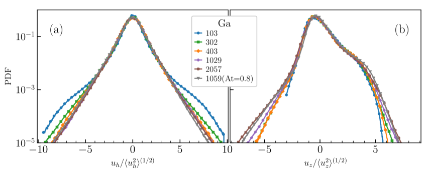
Figure 4: The probability distribution function of the (a) horizontal and (b) the vertical component of the liquid velocity fluctuations at different Ga.

I.2 Velocity power spectra

The two-point velocity correlations can be characterized in Fourier space using the second rank spectral tensor

$$C^{\alpha\beta}(\bm{k})\equiv\left\langle\hat{{u}}^{\alpha}(\bm{k})\hat{{u}}^{\beta}(-\bm{k})\right\rangle,$$ (5)

where indices $\alpha,\beta=x,y,z$. The power spectrum of velocity fluctuations can be rewritten in terms of the spectral tensor as

$$E(k)=\frac{1}{2}\sum_{\bm{k}}C^{\alpha\alpha}({\bm{k}})\delta(|\bm{k}|-k).$$ (6)

As the anisotropy in bubbly flows is because the buoyancy force is along the $\hat{z}$-direction. Therefore, we use the axisymmetric turbulence formalism outlined in [27] and construct two unit vectors orthogonal to ${\bm{k}}$:

$$\bm{e}_{\rm 1}\equiv\frac{\bm{k}\times\hat{z}}{\lvert\bm{k}\times\hat{z}\rvert}\/,\quad{\rm and}~{}\bm{e}_{\rm 2}\equiv\frac{\bm{k}\times(\bm{k}\times\hat{z})}{\lvert\bm{k}\times(\bm{k}\times\hat{z})\rvert}\/.$$ (7)

The spectral tensor can be written in terms of the $\bm{e}_{\rm 1}$ and $\bm{e}_{\rm 2}$ vectors as

$$C^{\alpha\beta}(\bm{k})=A(\bm{k})e_{\rm 1}^{\alpha}e_{\rm 1}^{\beta}+B(\bm{k})e_{\rm 2}^{\alpha}e_{\rm 2}^{\beta},$$ (8)

with indices $\alpha,\beta=x,y,z$.

We evaluate $C^{\alpha\beta}(\bm{k})$ from our DNS, and use Eq. (7), and (8) to obtain

$$A(\bm{k}) =\frac{k_{y}^{2}C^{xx}(\bm{k})-2k_{x}k_{y}\operatorname{Re}[C^{xy}(\bm{k})]+k_{x}^{2}C^{yy}(\bm{k})}{k_{x}^{2}+k_{y}^{2}},\quad~{}\rm{and}\/$$

$$B(\bm{k}) =C^{zz}(\bm{k})\frac{k^{2}}{k_{x}^{2}+k_{y}^{2}}.$$

Note that the function $A(\bm{k})$ gets contribution only from the horizontal velocity fluctuations, whereas $B(\bm{k})$ only depends on vertical velocity fluctuations. By performing the angular averaging, similar to Eq. (2) (main document) we define the one-dimensional spectra

$$a(k) =\frac{1}{2}\sum_{\bm{k}}A({\bm{k}})\delta(|\bm{k}|-k)~{}{\rm and~{}}$$ (9)

$$b(k) =\frac{1}{2}\sum_{\bm{k}}B({\bm{k}})\delta(|\bm{k}|-k).$$ (10)

We expect $a(k)=b(k)$ for homogeneous, isotropic turbulence. In Fig. (5) we compare different spectrum for $\mbox{Ga}=302$ and $2057$. The flow isotropy is higher at scales larger than the bubble diameter. For small $\mbox{Ga}=302$, most of the contribution to the energy spectrum comes from the vertical velocity fluctuations ($E(k)\approx 2b(k)>a(k)$). However, all the spectrum show identical scaling behaviour. On increasing the $\mbox{Ga}=2057$, we find that $E(k)\approx 2a(k)\approx 2b(k)$ for scales larger than the bubble diameter indicating isotropization of small scale fluctuations. Therefore, we conclude that Eq. (2) (main document) is a good indicator to study the scaling behaviour of velocity fluctuations in bubbly flows.

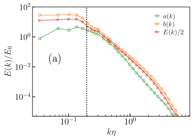
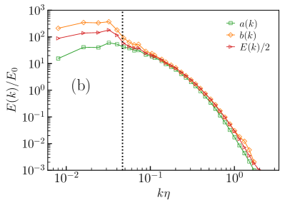
Figure 5: Anisotropic decomposition of velocity power spectra for (a) $\mbox{Ga}=302$, (b) $\mbox{Ga}=2057$. Vertical line show the wave mode corresponding to the bubble diameter.

II Derivation of the scale-by-scale budget equations

In this section, we detail the complete derivation of the scale-by-scale energy budget equations. Following Ref. [29, 30, 17, 33], for any field, $\psi(\bm{x})$ we obtain the corresponding field filtered at scale $K$ as,

$${\psi}_{K}(\bm{x}) \equiv\int\exp(i\bm{q}\cdot\bm{x})G_{\rm K}(\bm{q})\hat{\psi}({\bm{q}}){\mathop{{\rm d}\bm{q}}}\/,\quad\text{where,}$$ (11a)

$$G_{\rm K}(\bm{q}) \equiv\exp\left(-{\pi^{2}q^{2}\over 24K^{2}}\right)\/$$ (11b)

where $\hat{\psi}(\bm{q})$ is the Fourier transforms of $\psi$, and $G_{\rm K}$ is a low-pass filtering kernel which is smooth in both physical and Fourier space. As we are dealing with a flow with density fluctuations, we define Favre filtered field ${\widetilde{\psi}_{K}}={(\rho\psi)}_{K}/{\rho}_{K}$ [33, 34].

We define the cumulative energy flux through scale $K$ as $\mathcal{E}_{K}={1\over 2}\left\langle{\rho}_{K}\mid\widetilde{\bm{u}}_{K}\mid^{2}\right\rangle$, such that the spectrum $E(k)\sim(1/\rho_{2})\partial_{K}\mathcal{E}_{K}\mid_{K=k}$. In the statistically stationary state $\partial_{t}\mathcal{E}_{K}=0$. Thus, from the Navier-Stokes equation Eqs. (1) (main document), and following the procedure outlined in Refs. [29, 34] we obtain the following scale-by-scale kinetic energy budget equation in the statistically stationary state:

$$\Pi_{K} +\mathscr{F}^{\sigma}_{K}-\mathscr{P}_{K}=-\mathscr{D}_{K}+\mathscr{F}^{\rm g}_{K}\/,\text{where}$$ (12a)

$$\Pi_{K} \equiv-\left\langle{\rho}_{K}{\partial^{\beta}\widetilde{u}_{K}^{\alpha}}\tau^{\alpha\beta}_{K}\right\rangle\/,$$ (12b)

$$\mathscr{F}^{\sigma}_{K} \equiv-\left\langle\widetilde{\bm{u}}_{K}\cdot{{\bm{F}}_{K}^{\sigma}}\right\rangle\/,$$ (12c)

$$\mathscr{P}_{K} \equiv-\left\langle\widetilde{\bm{u}}_{K}\cdot{{(\nabla p)}_{K}}\right\rangle\/,$$ (12d)

$$\mathscr{D}_{K} \equiv 2\mu\left\langle\partial^{\beta}\widetilde{u}_{K}^{\alpha}{S}_{K}^{\alpha\beta}\right\rangle\/,$$ (12e)

$$\mathscr{F}^{\rm g}_{K} \equiv\left\langle\widetilde{\bm{u}}_{K}\cdot{\bm{F}}_{K}^{g}\right\rangle\/,\text{where}$$ (12f)

$$S^{\alpha\beta} \equiv\frac{1}{2}\left[\partial^{\alpha}u^{\beta}+\partial^{\beta}u^{\alpha})\right]\/,\text{and}$$ (12g)

$$\tau^{\alpha\beta}_{K} \equiv\widetilde{(u^{\alpha}u^{\beta})}_{K}-\widetilde{u}_{K}^{\alpha}\widetilde{u}_{K}^{\beta}.$$ (12h)

In Eq. (12a), $\Pi_{K}$ is the advective flux, $\tau_{K}$ is the Reynolds stress tensor. In bubbly flows, the “baropycnal work” $\mathscr{P}_{K}$ and the surface tension term $\mathscr{F}^{\sigma}_{K}$ provide alternate routes for nonlinear energy transfers. The baropycnal term has contributions from the barotropic generation of strain and baroclinic generation of vorticity due to density variations [34]. The other terms in Eq. (12a) are the cumulative injection rate up to wavenumber $K$ due to buoyancy $\mathscr{F}^{\rm g}_{K}$, and dissipation rate up to wavenumber $K$, $\mathscr{D}_{K}$.

At low Atwood number, we can employ Boussinesq approximation. Therefore $\widetilde{{\bm{u}}}_{K}\approx{\bm{u}}_{K}$, similarly $\mathcal{E}_{K}\approx{1\over 2}\rho_{\rm a}\left\langle\mid{\bm{u}}_{K}\mid^{2}\right\rangle$, and the power spectrum $E(k)=(1/\rho_{\rm a})\partial_{K}\mathcal{E}_{K}\mid_{K=k}$. The other terms in the budget equation reduces to:

$$\Pi_{K} \equiv-\rho_{\rm a}\left\langle{S}_{K}^{\alpha}\beta\tau^{\alpha\beta}_{K}\right\rangle\/,$$ (13a)

$$\mathscr{F}^{\sigma}_{K} \equiv-\left\langle{\bm{u}}_{K}\cdot{{\bm{F}}_{K}^{\sigma}}\right\rangle\/,$$ (13b)

$$\mathscr{P}_{K} =0\/,$$ (13c)

$$\mathscr{D}_{K} \equiv 2\mu\left\langle{S}_{K}^{\alpha\beta}{S}_{K}^{\alpha\beta}\right\rangle\/,$$ (13d)

$$\mathscr{F}^{\rm g}_{K} \equiv\left\langle{\bm{u}}_{K}\cdot{\bm{F}}_{K}^{g}\right\rangle\/,\text{and}$$ (13e)

$$\tau^{\alpha\beta}_{K} \equiv{(u^{\alpha}u^{\beta})}_{K}-{u}_{K}^{\alpha}{u}_{K}^{\beta}.$$ (13f)

III Statistically stationary state

In Fig. (6), we show the time series of $E(t)=\overline{\bm{u}^{2}}/2$ for a time period over which we have averaged the data for a few representative simulations. Note that within the scope of the current section, $\overline{(\cdot)}$ represents spatial average.

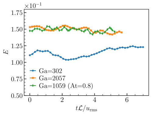
Figure 6: The time evolution of $E(t)$ for $\mbox{Ga}=302,2057$ at $\mbox{At}=0.04$ and $\mbox{Ga}=1059$ at $\mbox{At}=0.80$.

IV Resolution test

We show comparison of power spectra at $\mbox{At}=0.04$ $\mbox{Ga}=1029$ at resolution $N=480$ and $720$ in Fig. (7). Similarly we also show the spectra for high $\mbox{At}=0.8$ $\mbox{Ga}=1059$ at resolution $N=288$ and $504$. We find that in both the cases scaling ranges to be well resolved as the spectra at different resolution overlaps. We observe a kink at the tail of the spectra indicating very small scales at deep dissipation range are under-resolved. As the resolution is increased this kink gets pushed to at even smaller scales, extending the pseudo-turbulent scaling. The resolution required to resolve these scales in the deep dissipation range increases with Ga [16] and is beyond the scope of current work.

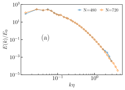
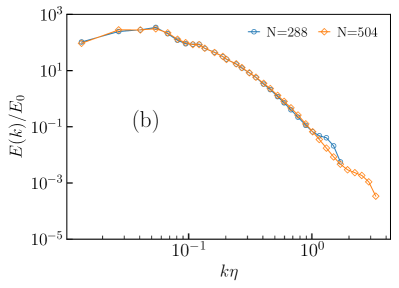
Figure 7: The comparison of velocity power spectrum for (a) $\mbox{At}=0.04,\mbox{Ga}=1029$ at spatial grid resolution of $N=480{~{}\rm and},720$, (b) $\mbox{At}=0.8,\mbox{Ga}=1059$ at spatial resolution of $N=288{~{}\rm and},504$.

References

- Batchelor [1953] G. Batchelor, The Theory of Homogeneous Turbulence (Cambridge University Press, 1953).
- Magnaudet and Eames [2000] J. Magnaudet and I. Eames, Annu. Rev. Fluid Mech. 32, 659–708 (2000).
- Mudde [2005] R. F. Mudde, Annu. Rev. Fluid Mech. 37, 393–423 (2005).
- Ceccio [2010] S. L. Ceccio, Annu. Rev. Fluid Mech. 42, 183–203 (2010).
- Risso [2018] F. Risso, Annu. Rev. Fluid Mech. 50, 25–48 (2018).
- Said [2019] E. Said, Annu. Rev. Fluid Mech. 51, 217 (2019).
- Mathai et al. [2020] V. Mathai, D. Lohse, and C. Sun, Annu. Rev. Fluid Mech. 11, 529–559 (2020).
- Lance and Bataille [1991] M. Lance and J. Bataille, J. Fluid Mech. 222, 95–118 (1991).
- Mercado et al. [2010] J. M. Mercado, D. G. Gómez, D. V. Gils, C. Sun, and D. Lohse, J. Fluid Mech. 650, 287–306 (2010).
- Riboux et al. [2010] G. Riboux, F. Risso, and D. Legendre, J. Fluid Mech. 643, 509–539 (2010).
- Ma et al. [2021] T. Ma, B. Ott, J. Fröhlich, and A. D. Bragg, J. Fluid Mech. 927, A16 (2021).
- Prakash et al. [2016] V. N. Prakash, J. M. Mercado, L. van Wijngaarden, E. Mancilla, Y. Tagawa, D. Lohse, and C. Sun, J. Fluid Mech. 791, 174–190 (2016).
- Alméras et al. [2017] E. Alméras, V. Mathai, D. Lohse, and C. Sun, J. Fluid Mech. 825, 1091–1112 (2017).
- Pandey et al. [2020] V. Pandey, R. Ramadugu, and P. Perlekar, J. Fluid Mech. 884, R6 (2020).
- Pandey et al. [2022] V. Pandey, D. Mitra, and P. Perlekar, J. Fluid Mech. 932, A19 (2022).
- Innocenti et al. [2021] A. Innocenti, A. Jaccod, S. Popinet, and S. Chibbaro, J. Fluid Mech. 918, A23 (2021).
- Frisch [1997] U. Frisch, Turbulence, A Legacy of A. N. Kolmogorov (Cambridge University Press, 1997).
- Popinet [2018] S. Popinet, Annu. Rev. Fluid Mech. 50, 1–28 (2018).
- Tryggvason et al. [2001] G. Tryggvason, B. Bunner, A. Esmaeeli, D. Juric, N. Al-Rawahi, W. Tauber, J. Han, S. Nas, and Y.-J. Jan, J. Comput. Phys. 169, 708 – 759 (2001).
- Chandrasekhar [1981] S. Chandrasekhar, Hydrodynamic and Hydromagnetic Stability (Dover Publications, 1981).
- Canuto et al. [2012] C. Canuto, M. Y. Hussaini, A. M. Quarteroni, and T. A. Zang, Spectral Methods in Fluid Dynamics (Springer-Verlag, 2012).
- Ramadugu et al. [2020] R. Ramadugu, V. Pandey, and P. Perlekar, Eur. Phys. J. E 43, 73 (2020).
- Cox and Matthews [2002] S. Cox and P. Matthews, J. Comput. Phys. 176, 430–455 (2002).
- Aniszewski et al. [2021] W. Aniszewski, T. Arrufat, M. Crialesi-Esposito, S. Dabiri, D. Fuster, Y. Ling, J. Lu, L. Malan, S. Pal, R. Scardovelli, G. Tryggvason, P. Yecko, and S. Zaleski, Comput. Phys. Commun. 263, 107849 (2021).
- Loisy et al. [2017] A. Loisy, A. Naso, and P. D. M. Spelt, J. Fluid Mech. 816, 94–141 (2017).
- Note [1] In the Kolmogorov theory of single phase turbulence, energy dissipation rate per unit mass is used. Since the problem at hand is multiphase flow, we use injection rate per unit volume. They are simply related to each other by the factor of mean density .
- Biferale and Procaccia [2005] L. Biferale and I. Procaccia, Phys. Rep. 414, 43 (2005).
- Note [2] See Supplementary Material for detailed step-by-step derivation, which includes Refs. [29, 30, 17, 33, 34].
- Pope [2012] S. Pope, Turbulent Flows (Cambridge University Press, 2012).
- Eyink [1995] G. Eyink, J. Stat. Phys. 78, 335–351 (1995).
- Verma [2019] M. K. Verma, Energy transfers in fluid flows (Cambridge University Press, 2019).
- Monin and Yaglom [1975] A. S. Monin and A. M. Yaglom, Statistical fluid mechanics, Volume-2: Mechanics of turbulence (MIT, Cambridge MA., 1975).
- Aluie [2013] H. Aluie, Physica D: Nonlinear Phenomena 247, 54 (2013).
- Lees and Aluie [2019] A. Lees and H. Aluie, Fluids 92, 1 (2019).
- Roghair et al. [2011] I. Roghair, J. M. Mercado, M. V. S. Annaland, H. Kuipers, C. Sun, and D. Lohse, Int. J. Multiph. Flow 37, 1093 – 1098 (2011).
- Ma et al. [2022] T. Ma, H. Hessenkemper, D. Lucas, and A. Bragg, J. Fluid Mech. 936, A42 (2022).
- Cano-Lozano et al. [2016] J. C. Cano-Lozano, C. Martinez-Bazan, J. Magnaudet, and J. Tchoufag, Phys. Rev. Fluid 1, 053604 (2016).