New results in AdS/CFT in low dimensions from massive Type IIA

Abstract

We review recent developments in the study of the AdS/CFT correspondence in low dimensions, focusing on the construction of AdS₃/CFT₂ and AdS₂/CFT₁ dual pairs in massive Type IIA string theory. We start discussing the $\text{AdS}_{3}\times S^{2}\times\text{CY}_{2}\times I$ solutions to massive IIA supergravity with $\mathcal{N}=(0,4)$ supersymmetry constructed in [1]. We review the 2d CFTs dual to these solutions, together with their defect interpretation as surface defects within 5d fixed point theories living in D4-D8 bound states. Next, we discuss the $\text{AdS}_{2}\times S^{3}\times\text{CY}_{2}\times I$ solutions with $\mathcal{N}=4$ supersymmetry constructed in [2]. We discuss the superconformal quantum mechanics dual to these solutions, that we interpret in terms of line defects realised as D0-D4 baryon vertices in 5d Sp(N) fixed point theories. We review a particular example in this class of solutions, constructed through non-Abelian T-duality with respect to a non-compact isometry group, and discuss the possible embedding of a 3d black hole geometry constructed long ago via non-Abelian T-duality within this solution.

1 Introduction

The study of AdS₃ and AdS₂ spaces in String Theory has been of paramount importance towards achieving our current microscopical understanding of black holes. These spaces describe the geometries of extremal black holes close to the horizon, and through the AdS/CFT correspondence have associated dual CFTs where their microscopical degrees of freedom can be identified. The agreement between the field theory degrees of freedom and the Bekenstein-Hawking entropy represents one of the most important achievements of String Theory in the last decades.

Recently, remarkable progress has been gained in the construction of AdS₃ and AdS₂ solutions to Type II supergravities for which the dual CFTs have also been identified [1]-[26]. These represent explicit new AdS/CFT pairs where the black hole microscopical counting program can be carried out in detail. In the AdS₂/CFT₁ case the well-known problems related to the non-connectedness of the boundary of AdS₂ and the interpretation of the central charge of the dual super-conformal quantum mechanics (SCQM) have been circumvented through explicit constructions of SCQM whose degrees of freedom match the Bekenstein-Hawking entropy [20, 2, 22, 23, 24].

Low dimensional AdS spaces constitute as well promising candidates to holographic duals of CFTs describing defects within higher dimensional CFTs. Notable examples of such realisations have been reported in [27, 28, 29, 30, 31, 32, 33, 34, 35, 36, 37, 38, 39, 40, 41, 19, 21, 42, 24]. In these realisations the brane set-ups in which the defect CFTs live are interpreted as brane intersections ending on bound states, which are described close to the horizon by higher dimensional AdS spaces. The brane intersections break some of the isometries of these higher dimensional spaces, giving rise to lower dimensional AdS spaces in the near horizon limit. These lower dimensional spaces are dual to low dimensional CFTs, that find an interpretation as defect CFTs within the higher dimensional CFTs living in the bound states on which the brane intersections end.

In these proceedings we will report on recent progress in the construction of AdS₃/CFT₂ and AdS₂/CFT₁ pairs in massive Type IIA supergravity while paying special attention to the description of the CFTs and their defect interpretation. The AdS solutions are foliations of $\text{AdS}_{3}\times S^{2}$ or $\text{AdS}_{2}\times S^{3}$ times a $\text{CY}_{2}$ over an interval, preserving 4 supersymmetries. Remarkably, the CFTs dual to general subclasses of these solutions have been shown to admit quiver descriptions in the UV which have been used to compute their degrees of freedom, which have been shown to match the holographic computations. These solutions thus constitute well-defined string theory settings where computations such as the corrections to the entropy of five and four dimensional black holes can be performed.

The approach taken in the construction of the AdS₂ solutions is to apply double analytical continuation techniques on the AdS₃ solutions. Compared to other approaches in the literature (see for instance [20, 22, 24]) this allows to construct AdS₂ spaces unrelated to AdS₃ ones, and therefore dual to SCQMs that do not occur as discrete light-cone compactifications of 2d CFTs [43, 44]. Yet, the explicit dual pairs that we will review show that it is possible to compute the SCQM central charge from a formula inherited from 2d. This is a striking result that deserves more detailed investigation.

In this article we will also put our focus on the interpretation of the new dual pairs as describing defect CFTs within the 5d Sp(N) fixed point theories living in D4-D8 bound states [45], whose near horizon geometry is the Brandhuber-Oz AdS₆ solution to massive Type IIA supergravity [46]. The approach that we take is to relate (a subset of) our solutions with the uplift to massive IIA of the AdS₃ and AdS₂ domain wall solutions to 6d minimal gauged supergravity obtained in [38, 39, 40]. These solutions asymptote locally to the AdS₆ vacuum in the UV, while they are singular in the IR, due to the presence of lower dimensional brane intersections. Thus, they can be interpreted as holographic duals of surface (for AdS₃) or line (for AdS₂) defect CFTs within the 5d Sp(N) fixed point theory dual to the AdS₆ vacuum.

The paper is organised as follows. We start in section 2 by reviewing the $\text{AdS}_{3}\times S^{2}\times\text{CY}_{2}\times I$ solutions constructed in [1], with a focus on the subclass for which the dual 2d CFT was identified in [11, 12, 13]. Then in subsection 2.2 we describe the defect interpretation of these solutions within the 5d Sp(N) fixed point theory, found in [19]. In section 3 we turn to the study of the $\text{AdS}_{2}\times S^{3}\times\text{CY}_{2}\times I$ solutions constructed in [18, 2], with special focus on the subclass of solutions for which the dual SCQM was identified. We devote subsection 3.2 to review a solution in the AdS₂ class recently constructed in [23], by means of a non-Abelian T-duality (NATD) transformation acting on the $\text{AdS}_{3}\times S^{3}\times\text{CY}_{2}$ solution of Type IIB string theory. Contrary to previous applications of NATD as a solution generating technique in supergravity, the NATD takes place in this case with respect to a non-compact group of isometries, mapping the $\text{AdS}_{3}\times S^{3}\times\text{CY}_{2}$ space onto an $\text{AdS}_{2}\times I^{\prime}\times S^{3}\times\text{CY}_{2}$ solution contained in the class of [18, 2]. We try to connect the previous solution to a black hole geometry constructed in [47], when non-Abelian T-duality was first introduced at the level of the string worldsheet. This geometry was found by performing NATD on the principal chiral model with group SL(2,$\mathbf{R}$), as an illustration of the applicability of NATD with respect to non-compact isometry groups. Our results in this subsection show that this black hole geometry cannot be embedded within massive Type IIA supergravity using the class of solutions constructed in [18, 2]. These are new results in our search for valid string theory backgrounds where the black hole geometry constructed in [47] could be embedded. In subsection 3.3 we turn to the defect interpretation of (a subclass of) the $\text{AdS}_{2}\times S^{3}\times\text{CY}_{2}\times I$ solutions as line defects within the 5d Sp(N) fixed point theory, following [19]. Finally in section 4 we summarise the contents of this paper and sketch future new directions of investigation.

2 AdS₃/CFT₂ with (0,4) supersymmetries

In [1] a family of AdS${}_{3}\times$S² solutions to massive IIA supergravity with $\mathcal{N}=(0,4)$ supersymmetry and SU(2)-structure was constructed. These solutions are foliations of AdS${}_{3}\times$S${}^{2}\times$M₄ over an interval, where M₄ is either a CY₂ or a 4d Kähler manifold. Both cases were studied in detail in [1]. In this review article we will focus on the case M${}_{4}=$CY₂, referred as Class I in that reference.

The Neveu-Schwarz sector of this subclass of solutions reads, in string frame,

$$\begin{split}\mathrm{d}s^{2}&=\frac{u}{\sqrt{h_{4}h_{8}}}\bigg{(}\mathrm{d}s^{2}_{\text{AdS}_{3}}+\frac{h_{8}h_{4}}{\Delta}\mathrm{d}s^{2}_{\text{S}^{2}}\bigg{)}+\sqrt{\frac{h_{4}}{h_{8}}}\mathrm{d}s^{2}_{\text{CY}_{2}}+\frac{\sqrt{h_{4}h_{8}}}{u}\text{d}z^{2},\qquad\Delta=4h_{8}h_{4}+u^{\prime 2}\;,\\ e^{-\Phi}&=\frac{h_{8}^{\frac{3}{4}}}{2h_{4}^{\frac{1}{4}}\sqrt{u}}\sqrt{\Delta}\;,\qquad~{}~{}~{}~{}H_{3}=\frac{1}{2}\mathrm{d}\left(-z+\frac{uu^{\prime}}{\Delta}\right)\wedge\text{vol}_{\text{S}^{2}},\end{split}$$ (1)

where $\Phi$ is the dilaton and $H_{3}$ is the field strength of the Kalb-Ramond antisymmetric tensor, $B_{2}$. The warping functions $h_{8}$ and $u$ have support on the $z$ coordinate while $h_{4}$ has support on $(z,\text{CY}_{2})$. We have denoted $u^{\prime}=\partial_{z}u$, and the same for the functions $h_{4}$ and $h_{8}$ below. The background (1) is supported by the Ramond-Ramond (RR) fluxes,

$$\begin{split}F_{0}&=h_{8}^{\prime},\;\;\;\qquad F_{2}=-\frac{1}{2}\bigg{(}h_{8}-\frac{h^{\prime}_{8}u^{\prime}u}{\Delta}\bigg{)}\text{vol}_{\text{S}^{2}},\\[5.69054pt] F_{4}&=-\bigg{(}\mathrm{d}\left(\frac{uu^{\prime}}{2h_{4}}\right)+2h_{8}\text{d}z\bigg{)}\wedge\text{vol}_{\text{AdS}_{3}}-\partial_{z}h_{4}\text{vol}_{\text{CY}_{2}}-h_{8}(*_{4}d_{4}h_{4})\wedge dz.\end{split}$$ (2)

Additionally, supersymmetry demands

$$u^{\prime\prime}(z)=0,$$ (3)

and away from localised sources, the Bianchi identities demand,

$$h_{8}^{\prime\prime}(z)=0,\;\;\;\;\partial_{z}^{2}h_{4}+h_{8}\nabla^{2}_{\text{CY}_{2}}h_{4}=0.$$ (4)

It was shown in [1] that the background defined by (1)-(2) is a solution of massive IIA supergravity preserving $(0,4)$ supersymmetries as long as the $h_{4},h_{8},u$ functions satisfy the conditions (3)-(4).

The Page fluxes, defined as $\hat{F}=e^{-B_{2}}\wedge F$, are given by,

$$\begin{split}\hat{F}_{0}&=h_{8}^{\prime},\qquad\qquad\hat{F}_{2}=-\frac{1}{2}\bigg{(}h_{8}-h_{8}^{\prime}(z-2\pi k)\bigg{)}\text{vol}_{\text{S}^{2}},\\ \hat{F}_{4}&=-\bigg{(}\partial_{z}\left(\frac{uu^{\prime}}{2h_{4}}\right)+2h_{8}\bigg{)}\text{d}z\wedge\text{vol}_{\text{AdS}_{3}}-\partial_{z}h_{4}\text{vol}_{\text{CY}_{2}}-h_{8}(*_{4}d_{4}h_{4})\wedge dz.\end{split}$$ (5)

Here we have taken into account large gauge transformations of $B_{2}$ of parameter $k$, $B_{2}\to B_{2}+{\pi k}\text{vol}_{\text{S}^{2}}$, for $k=0,1,....,P$, that ensure that it remains in the fundamental region,

$$\frac{1}{4\pi^{2}}|\int_{\text{S}^{2}}B_{2}|\in[0,1].$$ (6)

These transformations are performed every time a $z$-interval $z\in[2\pi k,2\pi(k+1)]$ is crossed.

In the case in which $h_{4}$ does not depend on the coordinates of the $\text{CY}_{2}$, the conditions (4) leave us with linear functions for both $h_{8}$ and $h_{4}$. The analysis of the dual field theory carried out in [11, 12, 13] considered functions of the form,

$$h_{4}(z)\!=\;\!\!\left\{\begin{array}[]{cccrcl}\frac{\beta_{0}}{2\pi}z&0\leq z\leq 2\pi,&\\ \alpha_{k}\!+\!\frac{\beta_{k}}{2\pi}(z-2\pi k)&~{}~{}2\pi k\leq z\leq 2\pi(k+1),&~{}~{}k=1,...,P-1\\ \alpha_{P}-\frac{\alpha_{P}}{2\pi}(z-2\pi P)&~{}~{}2\pi P\leq z\leq 2\pi(P+1),&\end{array}\right.$$ (10)

$$h_{8}(z)=\left\{\begin{array}[]{cccrcl}\frac{\nu_{0}}{2\pi}z&0\leq z\leq 2\pi,&\\ \mu_{k}+\frac{\nu_{k}}{2\pi}(z-2\pi k)&~{}~{}2\pi k\leq z\leq 2\pi(k+1),&~{}~{}k=1,...,P-1\\ \mu_{P}-\frac{\mu_{P}}{2\pi}(z-2\pi P)&~{}~{}2\pi P\leq z\leq 2\pi(P+1),&\end{array}\right.$$ (14)

which, being piecewise linear, allow for D4 and D8 sources in the background, as implied by the expressions for $\hat{F}_{4}$ and $\hat{F}_{0}$ in (5). Here it has been imposed that $h_{4}$ and $h_{8}$ vanish at $z=0$, where the space begins, and at $z=2\pi(P+1)$, where the space ends. The singularity structure of the metric and dilaton at these points is that of a superposition of D2-branes wrapped on $\text{AdS}_{3}$ and smeared on the $\text{CY}_{2}\times\text{S}^{2}$, and D6-branes wrapped on $\text{AdS}_{3}\times\text{CY}_{2}$. In turn, $u$ needs to be continuous for preservation of supersymmetry. In this paper we will consider the simplest case $u^{\prime}=0$. Those readers interested in the $u^{\prime}\neq 0$ case are referred to [13, 48].

Imposing the continuity of the Neveu-Schwarz sector across the various intervals one finds that the quantities $(\alpha_{k},\beta_{k},\mu_{k},\nu_{k})$ must satisfy,

$$\alpha_{k}=\sum_{j=0}^{k-1}\beta_{j},~{}~{}~{}\mu_{k}=\sum_{j=0}^{k-1}\nu_{j}.$$ (15)

In turn, the quantised charges are given, in the $[z_{k},z_{k+1}]$ interval, by

$$Q_{\text{D2}}^{(k)}=\alpha_{k}=\sum_{j=0}^{k-1}\beta_{j},\qquad Q_{\text{D6}}^{(k)}=\mu_{k}=\sum_{j=0}^{k-1}\nu_{j}$$

$$Q_{\text{D4}}^{(k)}=\beta_{k},\qquad Q_{\text{D8}}^{(k)}=\nu_{k},\qquad Q_{\text{NS5}}^{(k)}=1,$$ (16)

which implies that $(\alpha_{k},\beta_{k},\mu_{k},\nu_{k})$ must be integer numbers.

In the next subsection we briefly summarise the two dimensional CFTs proposed in [11, 12] as duals to the family of solutions given by (1)-(2) with $h_{4}$, $h_{8}$ given by (10)-(14).

2.1 Two dimensional dual CFTs

	x0	x1	x2	x3	x4	x5	x6	x7	x8	x9
D2	x	x					x
D4	x	x						x	x	x
D6	x	x	x	x	x	x	x
D8	x	x	x	x	x	x		x	x	x
NS5	x	x	x	x	x	x

Table 1: Brane set-up underlying the background given by (1)-(4). $(x^{0},x^{1})$ are the directions where the two dimmensional CFT lives. The directions $(x^{2},\dots,x^{5})$ span the CY₂, on which the D6- and the D8-branes are wrapped. The coordinate $x^{6}$ is the direction associated with $z$. Finally $(x^{7},x^{8},x^{9})$ are the orthogonal directions realising the SO(3) R-symmetry.

The branes that underlie the background defined by equations (1)-(4) are distributed as indicated in Table 1. The D2- and D6-branes play the role of colour branes, while the D4- and D8-branes are flavour branes. This interpretation is supported by the study of the Bianchi identities, given by

$$\text{d}F_{0}=\sum_{k=1}^{P}\Bigl{(}\frac{\nu_{k-1}-\nu_{k}}{2\pi}\Bigr{)}\delta(z-2\pi k)\text{d}z$$

$$\text{d}{\hat{F}}_{4}=\sum_{k=1}^{P}\Bigl{(}\frac{\beta_{k-1}-\beta_{k}}{2\pi}\Bigr{)}\delta(z-2\pi k)\text{d}z\wedge\text{vol}_{\text{CY}_{2}}\,,$$ (17)

which show that at the points $z=2\pi k$ there are D4 and D8 localised sources.

Figure 1: Hanany-Witten brane set-up associated to the solutions with $h_{4}$, $h_{8}$ functions given by (10)-(14). The horizontal lines represent colour branes, in our case D2 and D6 branes, vertical lines represent NS5-branes and the crosses are flavour branes (D4- and D8-branes).

The previous information can be codified in the Hanany-Witten brane set-up depicted in Figure 1. As shown in [11, 12, 26], the 2d field theories living in these brane intersections are represented by the quivers depicted in Figure 2, whose dynamics conjecturally flow in the IR to CFTs with small ${\cal N}=(0,4)$ supersymmetry, dual to the AdS₃ solutions. The 2d field theory lives in the D2 and D6 colour branes and there are adequate flavour groups coming from D4 and D8 branes, that give rise to non-anomalous quivers.

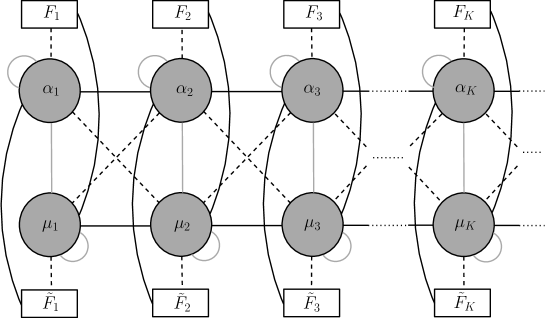
Figure 2: Quivers encoding the two dimensional field theories living in the D2-D4-D6-D8-NS5 brane intersections depicted in Figure 1.

The quiver dynamics was first studied in [11, 12], and later analysed in deeper detail in [26], where the explicit quantisation of the open strings connecting the different branes in the set-up was carried out. This detailed analysis led to corrections to some of the results in [11, 12], not changing however significantly the main conclusions in these papers. The multiplets that arise from the quantisation of open strings are summarised in Table 2. The quivers depicted in Figure 2 are then described in terms of $(0,4)$ vector multiplets and $(0,4)$ adjoint hypermultiplets, associated to the gauge nodes (depicted by circles and grey lines starting and ending on the same gauge group, respectively), $(4,4)$ twisted hypermultiplets in the bifundamental representation of two gauge groups (depicted by black lines), (0,4) bifundamental hypermultiplets (grey lines) and (0,2) bifundamental Fermi multiplets (dashed lines).

String	Interval	Multiplet	Representation
D2-D2	Same	$\mathcal{N}=(0,4)$ vector $+$ $\mathcal{N}=(0,4)$ hyper	Adjoint
D2-D2	Adjacent	$\mathcal{N}=(4,4)$ twisted hyper	bi-fundamental
D6-D6	Same	$\mathcal{N}=(0,4)$ vector $+$ $\mathcal{N}=(0,4)$ hyper	Adjoint
D6-D6	Adjacent	$\mathcal{N}=(4,4)$ twisted hyper	bi-fundamental
D2-D6	Same	$\mathcal{N}=(0,4)$ hyper	bi-fundamental
D2-D6	Adjacent	$\mathcal{N}=(0,2)$ Fermi	bi-fundamental
D2-D4	Same	$\mathcal{N}=(4,4)$ twisted hyper	bi-fundamental
D4-D6	Same	$\mathcal{N}=(0,2)$ Fermi	bi-fundamental
D2-D8	Same	$\mathcal{N}=(0,2)$ Fermi	bi-fundamental
D6-D8	Same	$\mathcal{N}=(4,4)$ twisted hyper	bi-fundamental

Table 2: Summary of the multiplets arising from the different strings stretching between branes in the brane set-up. The interval column determines whether the branes lie in the same interval or in adjacent intervals. For strings that do not contribute massless modes we have ignored their contribution in the table, for example D4-D4 strings.

As discussed in [11, 12, 26], the cancellation of gauge anomalies constrains, for generic U($\alpha_{k}$) and U($\mu_{k}$) colour groups, the ranks of the respective flavour groups to be,

$$F_{k}=\nu_{k-1}-\nu_{k},\;\;\;\;\tilde{F}_{k}=\beta_{k-1}-\beta_{k},$$ (18)

exactly as implied by (17). Moreover, the field theory and holographic central charges can be shown to match in the holographic limit. Indeed, the right-moving central charge of the IR SCFT can be calculated using its relation with the U$(1)_{R}$ current two-point function,

$$c_{R}=3\text{Tr}[\gamma^{3}Q_{R}^{2}],$$ (19)

where the trace is over the Weyl fermions of the theory and $\gamma^{3}$ is the chirality matrix in 2d. Keeping in mind the R-charges and fermion content of the different multiplets, summarised in Table 3, this leads to

$$c_{R}=6(n_{hyp}-n_{vec}),$$ (20)

where $n_{hyp}$ is the number of $(0,4)$ hypermultiplets and $n_{vec}$ is the number of $(0,4)$ vector multiplets. Note that (0,4) twisted hypermultiplets and (0,2) Fermi multiplets do not contribute to the R-symmetry anomaly, and therefore they do not contribute either to the central charge. For the quivers depicted in Figure 2 the central charge is then given by

$$c_{R}=6\sum_{k=1}^{P}\alpha_{k}\mu_{k}.$$ (21)

Multiplet	$(0,2)$ Origin	Number of Fermions	Chirality	R-charge of Fermion
$(0,4)$ hyper	2 $\times$ Chiral	2	R.H.	-1
$(0,4)$ twisted hyper	2$\times$ Chiral	2	R.H.	0
$(0,4)$ vector	(0,2) vector	1	L.H.	1
	(0,2) Fermi	1	L.H.	1
$(0,2)$ Fermi	-	1	L.H.	0

Table 3: R-charges and fermion content of the multiplets.

In turn, the holographic central charge for the geometries defined by (1) is given by

$$c_{hol}=\frac{3\pi}{2G_{N}}\text{Vol}_{\text{CY}_{2}}\int_{0}^{2\pi(P+1)}h_{4}h_{8}\text{d}z=\frac{3}{\pi}\int_{0}^{2\pi(P+1)}{h}_{4}h_{8}\text{d}z.$$ (22)

Here we have used that $G_{N}=8\pi^{6}$, with $g_{s}=\alpha^{\prime}=1$, and that $\text{Vol}_{\text{CY}_{2}}=16\pi^{4}$. For the functions $h_{4}$, $h_{8}$ displayed in (10)-(14) this gives

$$c_{hol}=\sum_{k=1}^{P}\Bigl{(}6\alpha_{k}\mu_{k}+3(\alpha_{k}\nu_{k}+\beta_{k}\mu_{k})+2\beta_{k}\nu_{k}\Bigr{)}\,.$$ (23)

As discussed in [26], this quantity has to be matched with the combination of left-moving and right-moving central charges of the field theory,

$$c_{hol}=\frac{c_{L}+c_{R}}{2}.$$ (24)

The left-moving central charge can be computed from the field theory using that

$$c_{L}-c_{R}=\text{Tr}\gamma^{3}.$$ (25)

This gives for the quivers depicted in Figure 2,

$$c_{L}-c_{R}=\sum_{k=1}^{P}\Bigl{(}\alpha_{k}(\mu_{k+1}-\mu_{k})+\mu_{k}(\alpha_{k+1}-\alpha_{k})\Bigr{)},$$ (26)

and finally

$$\frac{c_{L}+c_{R}}{2}=\sum_{k=1}^{P}\Bigl{(}6\alpha_{k}\mu_{k}+\frac{1}{2}(\alpha_{k}(\mu_{k+1}-\mu_{k})+\mu_{k}(\alpha_{k+1}-\alpha_{k}))\Bigr{)}.$$ (27)

Comparing this expression to the expression (23) for the holographic central charge one can see that they agree exactly to leading order. As discussed in [26] it is expected that higher order corrections to the gravity computation will yield an exact matching between the two quantities.

In the next subsection we summarise the results found in [19], which show that a subclass of the previous solutions with $\text{CY}_{2}=T^{4}$ can be interpreted as describing two dimensional defects within the 5d CFT dual to the AdS₆ background of Brandhuber-Oz [46].

2.2 Defect interpretation

In [19] the full brane solutions whose near horizon geometries are the AdS${}_{3}\times S^{2}\times T^{4}\times I$ backgrounds discussed in the previous subsections were constructed. They were interpreted in terms of D2-NS5-D6 branes ending on D4-D8 bound states. Furthermore, a parametrisation was obtained that allowed to relate a subclass of the AdS₃ geometries to 6d domain walls that asymptote locally to AdS₆. This allowed to propose a dual interpretation of these AdS₃ solutions as surface defect CFTs within the 5d Sp(N) CFT dual to the Brandhuber-Oz AdS₆ background.

The brane intersection constructed in [19] reads

$$\begin{split}ds_{10}^{2}&=H_{\mathrm{D}4}^{-1/2}\,H_{\mathrm{D}8}^{-1/2}\,\left[H_{\mathrm{D}6}^{-1/2}\,H_{\mathrm{D}2}^{-1/2}\,ds^{2}_{\mathbb{R}^{1,1}}+H_{\mathrm{D}6}^{1/2}\,H_{\mathrm{D}2}^{1/2}\,H_{\mathrm{NS}5}(dr^{2}+r^{2}ds^{2}_{S^{2}})\right]\\ &+H_{\mathrm{D}4}^{1/2}\,H_{\mathrm{D}8}^{1/2}H_{\mathrm{D}6}^{-1/2}\,H_{\mathrm{D}2}^{-1/2}\,H_{\mathrm{NS}5}dz^{2}+H_{\mathrm{D}4}^{1/2}\,H_{\mathrm{D}8}^{-1/2}H_{\mathrm{D}6}^{-1/2}\,H_{\mathrm{D}2}^{1/2}(d\rho^{2}+\rho^{2}ds^{2}_{\tilde{S}^{3}})\,,\end{split}$$ (28)

and

$$\begin{split}&C_{3}=H_{\mathrm{D}8}\,H_{\mathrm{D}2}^{-1}\,\text{vol}_{\mathbb{R}^{1,1}}\wedge dz\,,\\ &C_{5}=H_{\mathrm{D}6}\,H_{\mathrm{NS}5}\,H_{\mathrm{D}4}^{-1}\,r^{2}\,\text{vol}_{\mathbb{R}^{1,1}}\wedge dr\wedge\text{vol}_{S^{2}}\,,\\ &C_{7}=H_{\mathrm{D}4}\,H_{\mathrm{D}6}^{-1}\,\rho^{3}\,\text{vol}_{\mathbb{R}^{1,1}}\wedge dz\wedge d\rho\wedge\text{vol}_{\tilde{S}^{3}}\,,\\ &B_{6}=H_{\mathrm{D}8}\,H_{\mathrm{D}4}\,H_{\mathrm{NS}5}^{-1}\,\rho^{3}\,\text{vol}_{\mathbb{R}^{1,1}}\wedge d\rho\wedge\text{vol}_{\tilde{S}^{3}}\,,\\ \vspace{0.4cm}&e^{\Phi}=H_{\mathrm{D}8}^{-5/4}\,H_{\mathrm{D}4}^{-1/4}\,H_{\mathrm{D}6}^{-3/4}\,H_{\mathrm{NS}5}^{1/2}\,H_{\mathrm{D}2}^{1/4}\,,\end{split}$$ (29)

with the $C_{9}$ potential for D8 branes defining the Romans mass as $F_{0}=m$.

In this intersection the D2 and the NS5 branes are taken to be smeared over the space transverse to the D4-branes, i.e. $H_{D2}=H_{D2}(r)$ and $H_{NS5}=H_{NS5}(r)$. The Bianchi identities read

$$\partial_{z}H_{\mathrm{D}8}=m\,,\qquad H_{\mathrm{NS}5}=H_{\mathrm{D}6}=H_{\mathrm{D}2}\,,\qquad\nabla^{2}_{\mathbb{R}^{3}_{r}}\,H_{\mathrm{NS}5}=0\,.$$ (30)

Imposing the relations (30), the Bianchi identities for $F_{(4)}$ and the equations of motion collapse to the equation describing the D4-D8 system [49],

$$\begin{split}&H_{\mathrm{D}8}\,\nabla_{T^{4}}^{2}\,H_{\mathrm{D}4}+\partial_{z}^{2}\,H_{\mathrm{D}4}=0\,.\end{split}$$ (31)

Finally a particular solution can be written down as

$$H_{\mathrm{NS}5}(r)=1+\frac{Q_{\mathrm{NS}5}}{r}\,,\qquad H_{\mathrm{D}6}(r)=1+\frac{Q_{\mathrm{D}6}}{r}\,,\qquad H_{\mathrm{D}2}(r)=1+\frac{Q_{\mathrm{D}2}}{r}\,,$$ (32)

where $Q_{\mathrm{D}6}=Q_{\mathrm{D}2}=Q_{\mathrm{NS}5}$ for (30) to be satisfied.

It was shown in [19] that this solution gives rise to the AdS${}_{3}\times S^{2}\times T^{4}\times I$ solutions discussed in the previous subsections (restricted to the case $u^{\prime}=0$) in the near horizon limit, i.e. when $r\rightarrow 0$. Furthermore, it was shown that the AdS₃ backgrounds asymptote locally to the AdS₆ vacuum associated to the D4-D8 system. This could be achieved through a change of variables that allowed to map the AdS₃ solutions to the uplift to massive IIA of the domain wall solutions to 6d $\mathcal{N}=(1,1)$ minimal gauged supergravity found in [38]. These domain wall solutions were shown to asymptote locally to the AdS₆ vacuum of 6d supergravity, and therefore, upon uplift, to the Brandhuber-Oz AdS₆ solution of massive IIA supergravity. This goes as follows.

In [38] the following 6d background was considered,

$$\begin{split}&ds^{2}_{6}=e^{2U(\mu)}\left(4\,ds^{2}_{AdS_{3}}+ds^{2}_{S^{2}}\right)+e^{2V(\mu)}d\mu^{2}\,,\\ &\mathcal{B}_{2}=b(\mu)\,\text{vol}_{S^{2}}\,,\\ &X_{6}=X_{6}(\mu)\,.\end{split}$$ (33)

This background is described by the set of BPS equations,

$$\begin{split}U^{\prime}=-2\,e^{V}\,f_{6}\,,\qquad X_{6}^{\prime}=2\,e^{V}\,X_{6}^{2}\,D_{X}f_{6}\,,\qquad b^{\prime}=\frac{e^{U+V}}{X_{6}^{2}}\,,\end{split}$$ (34)

together with the duality constraint

$$b=-\frac{e^{U}\,X_{6}}{m}\,,$$ (35)

and the superpotential $f_{6}$

$$f_{6}(m,g,X_{6})=\frac{1}{8}\Bigl{(}mX_{6}^{-3}+\sqrt{2}gX_{6}\Bigr{)},\qquad\text{with}\qquad m=\frac{\sqrt{2}}{3}g.$$ (36)

This flow preserves 8 real supercharges (BPS/2 in 6d). In order to obtain an explicit solution of (34), the parametrisation of the 6d geometry

$$e^{-V}=2\,X_{6}^{2}\,D_{X}f_{6}$$ (37)

was chosen. The system (34) could then be integrated out easily [38], to give

$$\begin{split}e^{2U}=&\ 2^{-1/3}g^{-2/3}\,\left(\frac{\mu}{\mu^{4}-1}\right)^{2/3}\ ,\qquad e^{2V}=8\,g^{-2}\,\frac{\mu^{4}}{\left(\mu^{4}-1\right)^{2}}\ ,\\ b=&\ -2^{4/3}\,3\,g^{-4/3}\,\frac{\mu^{4/3}}{(\mu^{4}-1)^{1/3}}\ ,\qquad\ X_{6}=\mu\ ,\end{split}$$ (38)

with $\mu$ running between 0 and 1.

One can see that for $\mu\rightarrow 1$ the 6d background is such that

$$\begin{split}\mathcal{R}_{6}=-\frac{20}{3}\,g^{2}+O(1-\mu)^{2/3}\,,\qquad X_{6}=&\ 1+O(1-\mu)\ ,\end{split}$$ (39)

where $\mathcal{R}_{6}$ is the scalar curvature. These are the curvature and scalar fields reproducing the AdS₆ vacuum. In turn, the 2-form gauge potential gives non-zero sub-leading contributions in this limit. This implies that the asymptotic geometry for $\mu\rightarrow 1$ is only locally AdS₆. In the opposite limit $\mu\rightarrow 0$, the 6d background is manifestly singular. This is due to the presence of the D2-NS5-D6 brane sources.

The uplift of the 6d domain wall solution reads

$$\begin{split}ds^{2}_{10}&=s^{-1/3}\,X_{6}^{-1/2}\,\Sigma_{6}^{1/2}\,e^{2U}\left(4\,ds^{2}_{AdS_{3}}+ds^{2}_{S^{2}}\right)+s^{-1/3}\,X_{6}^{-1/2}\,\Sigma_{6}^{1/2}e^{2V}d\mu^{2}\\ &+2g^{-2}s^{-1/3}\Sigma_{6}^{1/2}\,X_{6}^{3/2}\,d\xi^{2}+2g^{-2}\,X_{6}^{-3/2}\,\Sigma_{6}^{-1/2}\,s^{-1/3}\,c^{2}\,ds^{2}_{\tilde{S}^{3}}\ ,\\ F_{4}&=-\frac{4\sqrt{2}}{3}\,g^{-3}\,s^{1/3}\,c^{3}\,\Sigma_{6}^{-2}\,U\,d\xi\,\wedge\,\text{vol}_{\tilde{S}^{3}}-8\sqrt{2}\,g^{-3}\,s^{4/3}\,c^{4}\,\Sigma_{6}^{-2}\,X_{6}^{-3}\,X_{6}^{\prime}\,d\mu\,\wedge\,\text{vol}_{\tilde{S}^{3}}\\ &-8\,\sqrt{2}\,g^{-1}\,s^{1/3}\,c\,X_{6}^{4}\,b^{\prime}\,e^{U-V}\,d\xi\wedge\text{vol}_{AdS_{3}}-8\,m\,s^{4/3}\,b\,X_{6}^{-2}\,e^{U+V}\,d\mu\wedge\text{vol}_{AdS_{3}}\,,\\ F_{2}&=m\,s^{2/3}\,b\,\text{vol}_{S^{2}}\ ,\qquad H_{3}=s^{2/3}\,b^{\prime}\,d\mu\wedge\text{vol}_{S^{2}}+\frac{2}{3}\,s^{-1/3}\,c\,b\,d\xi\wedge\text{vol}_{S^{2}}\ ,\\ e^{\Phi}&=s^{-5/6}\,\Sigma_{6}^{1/4}\,X_{6}^{-5/4}\ ,\qquad F_{(0)}=m\,,\end{split}$$ (40)

with $c=\cos\xi$, $s=\sin\xi\,,\,\,\Sigma_{6}=X_{6}\,c^{2}+X_{6}^{-3}\,s^{2}$ and $U$ given by

$$U=X_{6}^{-6}s^{2}-3X_{6}^{2}c^{2}+4X_{6}^{-2}.$$ (41)

It was shown in [19] that the background (40) takes exactly the form of the AdS₃ solutions defined by (1)-(2), upon the change of coordinates

$$z=\frac{3\,s^{2/3}\,e^{U}\,X_{6}}{\sqrt{2}\,g\,Q_{\mathrm{NS}5}}\,,\qquad\rho=\frac{\sqrt{2}\,c\,e^{3U/2}}{g\,Q_{\mathrm{NS}5}^{3/2}\,X_{6}^{1/2}}\,.$$ (42)

The AdS₃ solution is then specified by the functions

$$H_{\mathrm{D}8}=\frac{s^{2/3}\,e^{U}\,X_{6}}{Q_{\mathrm{NS}5}}\,,\qquad H_{\mathrm{D}4}=\frac{Q_{\mathrm{NS}5}^{5}\,e^{-5U}}{\Sigma_{6}}\,,$$ (43)

which can be shown to satisfy the Bianchi identities given by (4), with $H_{D8}=h_{8}$ and $H_{D4}=h_{4}$.

We have thus shown that the AdS₃ backgrounds describing the near-horizon limit of D2-NS5-D6 branes ending on the D4-D8 brane system, reproduce locally the AdS₆ vacuum of [46] for $H_{\mathrm{D}8}$, $H_{\mathrm{D}4}$ given by (43). This vacuum geometry comes out thanks to a non-linear mixing of the $(z,\rho)$ coordinates, that relates the near-horizon geometry to a 6d domain wall admitting AdS₆ in its asymptotics. The presence of the 2-form does not allow however to globally recover the vacuum in this limit. This is seen explicitly at the level of the uplift (40), where one notes that the $F_{2}$ and $H_{3}$ fluxes break the isometries of the D4-D8 vacuum. This is the manifestation of the D2-NS5-D6 defect, that underlies as well the singular behaviour of the 6d domain wall in its IR regime.

In the next section we summarise a new class of AdS₂ solutions to massive Type IIA supergravity obtained from the solutions reviewed in this section via a double analytical prescription. We describe the superconformal quantum mechanics dual to these solutions, together with a very similar defect interpretation within AdS₆ to the one presented in this subsection.

3 AdS₂/CFT₁ with 4 supersymmetries

We start this section reviewing the new class of AdS${}_{2}\times$S${}^{3}\times$CY${}_{2}\times$I solutions to massive Type IIA supergravity studied in [18, 2]. These solutions were obtained via a double analytical continuation from the solutions reviewed in Section 2. This double analytical continuation changes the AdS₃ and S² factors of the backgrounds in (1)-(2) as,

$$\begin{split}&\text{d}s_{\text{AdS}_{3}}^{2}\to-\text{d}s_{\text{S}^{3}}^{2},\qquad\text{d}s_{\text{S}^{2}}^{2}\to-\text{d}s_{\text{AdS}_{2}}^{2}.\end{split}$$ (44)

In order to get well-defined supergravity fields the $h_{8},h_{4}$ and $u$ functions need to be also analytically continued as,

$$\begin{split}u\to-iu,\qquad h_{4}\to ih_{4},\qquad h_{8}\to ih_{8},\end{split}$$ (45)

together with $z\to iz$. In this way, one finds a class of AdS${}_{2}\times$S${}^{3}\times$CY${}_{2}\times$I solutions to massive Type IIA supergravity with 4 supercharges, with NS-NS sector given by

$$\begin{split}&\text{d}s^{2}=\frac{u}{\sqrt{h_{4}h_{8}}}\left(\frac{h_{4}h_{8}}{\tilde{\Delta}}\text{d}s^{2}_{\text{AdS}_{2}}+\text{d}s^{2}_{\text{S}^{3}}\right)+\sqrt{\frac{h_{4}}{h_{8}}}\text{d}s^{2}_{\text{CY}_{2}}+\frac{\sqrt{h_{4}h_{8}}}{u}\text{d}z^{2}\,,\qquad\tilde{\Delta}=4h_{4}h_{8}-u^{\prime 2},\\ &e^{-2\Phi}=\frac{h_{8}^{3/2}\tilde{\Delta}}{4h_{4}^{1/2}u}\,,\qquad\qquad B_{2}=-\frac{1}{2}\bigg{(}z+\frac{uu^{\prime}}{\tilde{\Delta}}\bigg{)}\text{vol}_{\text{AdS${}_{2}$}},\,\end{split}$$ (46)

and RR fluxes,

$$\begin{split}F_{0}&=h_{8}^{\prime}\,,\qquad F_{2}=-\frac{1}{2}\Big{(}h_{8}+\frac{h_{8}^{\prime}u^{\prime}u}{\tilde{\Delta}}\Big{)}\text{vol}_{\text{AdS${}_{2}$}}\,,\\ F_{4}&=\left(-\text{d}\bigg{(}\frac{u^{\prime}u}{2h_{4}}\bigg{)}+2h_{8}\text{d}z\right)\wedge\text{vol}_{\text{S}^{3}}-\partial_{z}h_{4}\text{vol}_{\text{CY${}_{2}$}}-h_{8}(*_{4}d_{4}h_{4})\wedge dz\,.\end{split}$$ (47)

These backgrounds are associated to D0-F1-D4-D4^′-D8 brane intersections that preserve $\mathcal{N}=4$ supersymmetries in one dimension. The corresponding brane set-up is depicted in Table 4.

	$x^{0}$	$x^{1}$	$x^{2}$	$x^{3}$	$x^{4}$	$x^{5}$	$x^{6}$	$x^{7}$	$x^{8}$	$x^{9}$
D0	x
D4	x	x	x	x	x
D$4^{\prime}$	x						x	x	x	x
D8	x	x	x	x	x		x	x	x	x
F1	x					x

Table 4: Brane set-up associated to the solutions (46)-(47). $x^{0}$ is the time direction of the ten dimensional spacetime, $x^{1},\dots,x^{4}$ are the coordinates spanned by the CY₂, $x^{5}$ is the direction where the F1-strings are stretched, and $x^{6},x^{7},x^{8},x^{9}$ are the coordinates where the SO$(4)$ R-symmetry is realised.

As in the AdS${}_{3}\times$S² solutions we restrict to the case in which $h_{4}$ does not depend on the coordinates of the $\text{CY}_{2}$. In this case the functions $h_{8}$, $h_{4}$ and $u$ have support on $z$, and satisfy the constraints imposed for supersymmetry and the Bianchi identities, away from localised sources, given by expressions (3) and (4), with $\nabla^{2}_{\text{CY}_{2}}h_{4}=0$. Thus $h_{8}$, $h_{4}$ and $u$ are again linear functions of $z$.

The Page fluxes are given by,

$$\begin{split}&\hat{F}_{0}=h_{8}^{\prime}\,,\qquad\qquad\hat{F}_{2}=-\frac{1}{2}\Big{(}h_{8}-h_{8}^{\prime}(z-2\pi k)\Big{)}\text{vol}_{\text{AdS${}_{2}$}}\,,\\ &\hat{F}_{4}=\left(2h_{8}\text{d}z-\text{d}\bigg{(}\frac{u^{\prime}u}{2h_{4}}\bigg{)}\right)\wedge\text{vol}_{\text{S${}^{3}$}}-h_{4}^{\prime}\text{vol}_{\text{CY${}_{2}$}}\,,\end{split}$$ (48)

where we have included large gauge transformations of $B_{2}$ of parameter $k$, $B_{2}\to B_{2}+\pi k\text{vol}_{\text{AdS}_{2}}$, as discussed in [2].

In the next subsection we summarise the dual SCQM of the backgrounds (46)-(47) for the choice of piecewise linear functions (10)-(14). We consider the case $u^{\prime}=0$ and discuss a concrete example with $u^{\prime}\neq 0$, constructed in [23], in subsection 3.2.

3.1 The dual quiver quantum mechanics

In [2] a proposal for a superconformal quantum mechanics living in the D0-D4-D$4^{\prime}$-D8-F1 brane set-up depicted in Table 4 was given in terms of a generalisation of the ADHM quantum mechanics described in [50]. The quantum mechanics was interpreted as describing the interactions between brane instantons and Wilson lines in the five dimensional theory with eight Poincaré supersymmetries living in the D4’-D8 brane intersection. For this purpose the complete D0-D4-D$4^{\prime}$-D8-F1 brane system was split into two subsystems, D4-D$4^{\prime}$-F1 and D0-D8-F1, that were first studied separately. The first subsystem was interpreted as describing BPS F1 Wilson lines introduced in the 5d theory living in the D4’-branes by D4-branes [53]. Similarly, the D0-D8-F1 subsystem was interpreted as describing F1 Wilson lines introduced in the worldvolume of the D8-branes by D0-branes [54]. Indeed, both subsystems are displayed exactly as in the D3-D5-F1 brane configuration that describes Wilson lines in antisymmetric representations in 4d $\mathcal{N}=4$ SYM, studied in [55, 56].

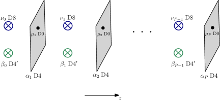
Figure 3: Hanany-Witten brane set-up associated to the solutions (46)-(47) for the choice of $h_{4}$, $h_{8}$ linear functions given by (10)-(14).

The quantised charges derived from the Page Fluxes (48) for the piecewise linear functions defined in (10)-(14) are given by,

$$Q_{\text{D4}}^{e(k)}=\alpha_{k}=\sum_{j=0}^{k-1}\beta_{j},\qquad Q_{\text{D0}}^{e(k)}=\mu_{k}=\sum_{j=0}^{k-1}\nu_{j}$$

$$Q_{\text{D4}^{\prime}}^{m(k)}=\beta_{k},\qquad Q_{\text{D8}}^{m(k)}=\nu_{k},\qquad Q_{\text{F1}}^{e(k)}=1,$$ (49)

in the $[2\pi k,2\pi(k+1)]$ interval. Here, the superscripts $e$ and $m$ indicate electric and magnetic charges, as discussed in [2].

The previous information can be summarised in the Hanany-Witten brane set-up depicted in Figure 3. In order to see the interpretation as Wilson lines one can map the brane configuration onto a F1-D3-NS5-NS7-D1 system in Type IIB via a T+S duality transformation, perform suitable Hanany-Witten moves and then go back to Type IIA via a further T-duality. This set of operations is carefully explained in [2]. One then obtains the configuration depicted in Figure 4, which can be interpreted as describing U$(\alpha_{k})$ and U$(\mu_{k})$ Wilson lines in the completely antisymmetric representations $(\beta_{0},\beta_{1},\dots,\beta_{k-1})$ of U$(\alpha_{k})$ and $(\nu_{0},\nu_{1},\dots,\nu_{k-1})$ of U$(\mu_{k})$, respectively. Given that the Wilson lines are in the completely antisymmetric representations the D4-D4’-F1 and D0-D8-F1 subsystems describe in fact baryon vertices [57].

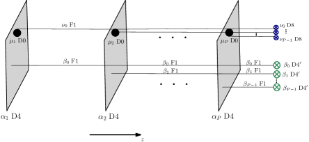
Figure 4: Brane configuration equivalent to the Hanany-Witten brane set-up depicted in Figure 3 after a T+S+T duality transformation and suitable Hanany-Witten moves.

This is consistent with an interpretation of the AdS₂ solutions as describing backreacted baryon vertices within the 5d ${\cal N}=1$ QFT living in the D4’-D8 branes. In this interpretation the dual SCQM arises in the very low energy limit of a D4’-D8 brane configuration, dual to a 5d QFT, where D4 and D0 brane baryon vertices are introduced. In the low energy limit the gauge symmetry on both the D4’ and D8 branes becomes global, shifting them from colour to flavour branes, with the D4 and D0 defect branes becoming the new colour branes of the backreacted configuration. This defect interpretation is in agreement with the results found in [19], that we summarise in subsection 3.3, where the AdS₂ geometries were shown to asymptote locally to the AdS₆ background of Brandhuber-Oz [46].

The superconformal quantum mechanics dual to the AdS₂ solutions was analysed in detail in [2]. In the UV it is encoded in the quiver construction depicted in Figure 5. In these quivers the gauge groups are associated to the colour D0- and D4-branes and the flavour groups to the D$4^{\prime}$- and D8-branes. The quantised charges are the ones computed in (49). The dynamics is described in terms of (4,4) vector multiplets (circles), (4,4) hypermultiplets in the adjoint representations (semicircles) and (4,4) hypermultiplets in the bifundamental representations (vertical lines). The connection between colour and flavour branes is through twisted (4,4) bifundamental hypermultiplets (bent lines) and (0,2) bifundamental Fermi multiplets (dashed lines). This follows directly from the analysis in Appendix B of [2]. Note that as in that reference we use 2d $\mathcal{N}=(0,4)$ notation to actually refer to the 1d $\mathcal{N}=4$ multiplets.

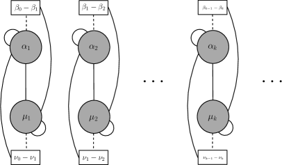
Figure 5: One dimensional quiver field theory whose IR limit is dual to the AdS₂ backgrounds (46)-(47).

Checking the agreement between the field theory and holographic central charges in SCQMs is less direct than in the 2d cases discussed in the previous section. Indeed, in a one dimensional field theory the energy momentum tensor has only one component, which must thus vanish if the theory is conformal. A possible way to interpret the central charge is then as counting the ground states of the conformal quantum mechanics. This quantity is the one that is compared to the holographic central charge, which can be computed as usual from the volume of the internal manifold. In our case it reads

$$c_{\text{hol}}=\frac{3V_{int}}{4\pi G_{N}}=\frac{3}{\pi}\int_{0}^{2\pi(P+1)}h_{4}h_{8}\;\text{d}z.$$ (50)

As discussed in [2], this result suggests that the same expression used in section 2.1 for the central charge of a 2d $\mathcal{N}=(0,4)$ CFT gives the number of ground states of a $\mathcal{N}=4$ SCQM, with $n_{hyp}$ counting now the number of (untwisted) 1d $\mathcal{N}=4$ hypermultiplets and $n_{vec}$ the number of 1d $\mathcal{N}=4$ vector multiplets. Again, perfect agreement was found in the holographic limit between this definition of the quantum mechanics central charge and the holographic central charge given by (50).

As emphasised in [2] this is a striking result, since the superconformal quantum mechanics dual to the AdS₂ solutions does not have a priori any relation to a 2d CFT. Comparing with results in the literature for the dimension of the Higgs branch of $\mathcal{N}=4$ quantum mechanics with gauge groups $\prod_{v}$ U$(N_{v})$ connected by bifundamentals [58], one can see that the expression $c_{cft}=6(n_{hyp}-n_{vec})$ may be interpreted as an extension of the formulas therein to more general $\mathcal{N}=4$ quivers including flavours. This is an interesting result that deserves further investigation.

3.2 A concrete AdS₂ example from non-Abelian T-duality

In this section we review a concrete example in the previous classification constructed in [23] via non-Abelian T-duality acting on a non-compact, freely acting, SL$(2,\mathbf{R})$ group.

The idea to study non-Abelian T-duality as a solution generating technique in supergravity was put forward in [59]. Since then, NATD has been successfully used in the context of holography to generate new AdS backgrounds (see [59]-[77] for a set of interesting examples and [17, 22] for more recent ones). Nevertheless, previous to [23] the dualisation had been carried out with respect to a freely acting SU(2) subgroup of the total symmetry group of the background.

The main purpose of [23] was to develop NATD as a solution generating technique in supergravity with respect to a freely acting non-compact SL$(2,\mathbf{R})$ group, and to apply the procedure to the D1-D5 near horizon system as an illustrative example. The resulting geometry was shown to belong to the AdS${}_{2}\times$S${}^{3}\times$CY₂ class of solutions given by (46)-(47). This allowed to construct an explicit completion of the quiver quantum mechanics proposed in [2].

The starting point is a Type II background with a NS-NS sector invariant under SL$(2,\mathbf{R})\times$ SL$(2,\mathbf{R})$,

$$\begin{split}ds^{2}&=\frac{1}{4}g_{\mu\nu}(x)L^{\mu}L^{\nu}+G_{i\mu}(x)dx^{i}L^{\mu}+G_{ij}(x)dx^{i}dx^{j},\qquad\Phi=\Phi(x)\\ B_{2}&=\frac{1}{8}b_{\mu\nu}(x)L^{\mu}\wedge L^{\nu}+\frac{1}{2}B_{i\mu}(x)dx^{i}\wedge L^{\mu}+B_{ij}(x)dx^{i}\wedge dx^{j},\end{split}$$ (51)

where $i,j=1,2,...,7$, and $L^{\mu}$ are the SL$(2,\mathbf{R})$ left-invariant Maurer-Cartan forms given by $L^{\mu}=-i\textrm{Tr}(t^{\mu}g^{-1}\text{d}g)$. A string propagating in such background is described by a sigma model that can be dualised with respect to the full SL$(2,\mathbf{R})$ isometry group acting on the left (or on the right), following the rules first given in [78]. The first step is to gauge the global symmetry, replacing ordinary derivatives with covariant derivatives, $dg\to Dg=dg-Ag$. Then, the Lagrange multiplier term $-i\textrm{Tr}(vF)$ needs to be added in order to enforce a flat connection, with $F=dA-[A,A]$ and $v$ a vector that takes values in the Lie algebra of the SL(2,$\mathbf{R}$) group. After integrating by parts the Lagrange multiplier term and fixing the gauge, that we do by setting $g=\mathbb{I}$, one obtains the NATD sigma model. As the variables parametrising the SL(2,$\mathbf{R}$) group are replaced by the Lagrange multipliers $\nu_{i}$, which by construction span the vector space $\mathbf{R}^{3}$, the AdS₃ space is replaced in a suitable parametrisation by AdS${}_{2}\times\mathbf{R}^{+}$. More details on this dualisation can be found in [47].

In [23] the dualisation was performed on the AdS${}_{3}\times$S${}^{3}\times$CY₂ geometry that arises as the near horizon limit of the D1-D5 system,

$$\begin{split}&ds^{2}=4L^{2}ds^{2}_{\text{AdS}_{3}}+M^{2}ds^{2}_{\text{CY}_{2}}+4L^{2}ds^{2}_{\text{S}^{3}},\qquad e^{2\Phi}=1,\qquad F_{3}=8L^{2}(\text{vol}_{\text{S}^{3}}+\text{vol}_{\text{AdS}_{3}}).\end{split}$$ (52)

In this case due care must be taken of the RR sector, which was dualised following the prescription in [59] (the reader is referred to [23] for more details). Parametrising the dual coordinates as $(z,\text{AdS}_{2})$ the background generated reads,

$$\begin{split}ds^{2}&=\frac{L^{2}z^{2}}{z^{2}-4L^{4}}ds^{2}_{\text{AdS}_{2}}+4L^{2}ds^{2}_{\text{S}^{3}}+M^{2}ds^{2}_{\text{CY}_{2}}+\frac{dz^{2}}{4L^{2}},\qquad e^{2\Phi}=\frac{4}{L^{2}(z^{2}-4L^{4})},\\ B_{2}&=-\frac{z^{3}}{2(z^{2}-4L^{4})}\text{vol}_{\text{AdS}_{2}},\qquad F_{0}=L^{2},\qquad F_{2}=-\frac{L^{2}z^{3}}{2(z^{2}-4L^{4})}\text{vol}_{\text{AdS}_{2}},\\ F_{4}&=-L^{2}(M^{4}\text{vol}_{\text{CY}_{2}}-2z\text{d}z\wedge\text{vol}_{\text{S}^{3}}).\end{split}$$ (53)

Notice that from the original SO$(2,2)\cong\textrm{SL}(2,\mathbf{R})_{L}\times\textrm{SL}(2,\mathbf{R})_{R}$ isometry group just one SL(2,$\mathbf{R}$) subgroup survives after the dualisation. This group is geometrically realised by a warped AdS${}_{2}\times\mathbf{R}^{+}$ subspace. As anticipated, it is easy to see that the background (53) fits locally in the class of AdS₂ solutions given by (46)-(47), with the choices,

$$\begin{split}u=4L^{4}M^{2}z,\qquad h_{4}=L^{2}M^{4}z,\qquad h_{8}=F_{0}z\,.\end{split}$$ (54)

In this case due to the $z$ dependence of $u$ there is a singularity at $z=z_{0}=2L^{2}$, where the metric and dilaton behave as

$$ds^{2}\sim\frac{a_{1}}{z-z_{0}}ds^{2}_{\text{AdS}_{2}}+a_{2}ds^{2}_{\text{S}^{3}}+M^{2}ds^{2}_{\text{CY}_{2}}+a_{3}dz^{2},\qquad\qquad e^{\Phi}\sim a_{4}(z-z_{0})^{-1/2}.$$ (55)

This behaviour can be interpreted in terms of F1-strings with AdS₂ worldvolume smeared over the $S^{3}$. The metric has the correct signature and the dilaton is well-defined when $z\in[z_{0},\infty)$.

The brane intersection associated to the new solution can be read from the Page fluxes, which are given by

$$\begin{split}\hat{F}_{0}=&L^{2},\quad\quad\quad\hat{F}_{2}=-L^{2}k\pi\text{vol}_{\text{AdS}_{2}},\quad\quad\quad\quad\hat{F}_{4}=-L^{2}(M^{4}\text{vol}_{\text{CY}_{2}}-2z\;\text{d}z\wedge\text{vol}_{\text{S}^{3}}),\end{split}$$ (56)

where we have taken into account the large gauge transformations $B_{2}\to B_{2}+\pi k\text{vol}_{\text{AdS}_{2}}$ as in [2]. These give rise to the D0-D4-D$4^{\prime}$-D8-F1 brane intersection depicted in Table 4. The D0 and D4-branes can then be interpreted as instantons carrying electric charge,

$$\begin{split}Q_{\text{D}0}^{e}=-k\;Q_{\text{D}8}^{m},\qquad Q_{\text{D}4}^{e}=-k\;Q_{\text{D}4^{\prime}}^{m}\;,\end{split}$$ (57)

while the D$4^{\prime}$ and D8-branes find an interpretation as magnetically charged branes where the instantons lie, with charges

$$\begin{split}Q_{\text{D}8}^{m}=2\pi L^{2},\qquad Q_{\text{D}4^{\prime}}^{m}&=-2\pi L^{2}M^{4},\qquad\end{split}$$ (58)

in the interval $[z_{k},z_{k+1}]$. On top of this there are fundamental strings electrically charged with respect to the 3-form $H_{3}$,

$$Q_{\text{F1}}^{e}=\frac{1}{(2\pi)^{2}}\int_{\text{AdS}_{2}\times\text{I}_{z}}H_{3}=\left.\frac{1}{\pi}B_{2}\;\right|_{z_{k}}^{z_{k+1}}=1.$$ (59)

The holographic central charge is obtained from the volume of the internal manifold, giving

$$\begin{split}&c_{\text{hol}}=\frac{3L^{4}M^{4}}{\pi}\int_{z_{0}}^{\infty}(z^{2}-4L^{4})\;\text{d}z.\end{split}$$ (60)

However, in order to obtain a finite value from this expression the dual background has first to be defined globally. The global completion proposed in [23] ended the geometry with F1-strings at a certain value $z_{2P}$, with $P\in\mathbb{Z}$, and glued the $h_{4}$, $h_{8}$ linear functions associated to the solution at $z_{P}$ in a symmetric fashion

$$\begin{split}\frac{h_{4}(z)}{L^{2}M^{4}}\!&=\!\!\;\!\!\left\{\begin{array}[]{cccrcl}z&z_{0}\leq z\leq z_{P}\;,&\\ z_{0}-(z-z_{2P})&~{}~{}z_{P}\leq z\leq z_{2P},&\end{array}\right.\quad\frac{h_{8}(z)}{L^{2}}=\!\!\;\!\!\left\{\begin{array}[]{cccrcl}z&z_{0}\leq z\leq{z_{P}},&\\ {z_{0}}-(z-z_{2P})&~{}~{}{z_{P}}\leq z\leq z_{2P}.&\end{array}\right.\end{split}$$ (61)

Indeed, one can check that the NS sector is continuous at $z_{P}$ when $z_{P}=\frac{z_{0}+z_{2P}}{2}$, thus leading to a symmetric configuration. The quantised charges associated to this choice of linear functions, displayed in Table 5, are such that the D0 and D4 charges increase linearly in the $0\leq k\leq P$ region while they decrease in the $P\leq k\leq 2P$ region.

	$Q^{m}_{\text{D8}}$	$Q^{e}_{\text{D0}}$	$Q^{m}_{\text{D4}^{\prime}}$	$Q^{e}_{\text{D4}}$
$0\leq k\leq P$	$2\pi L^{2}$	$k\;Q^{m}_{\text{D8}}$	$2\pi L^{2}M^{4}$	$k\;Q^{m}_{\text{D4}^{\prime}}$
$P\leq k\leq 2P$	$2\pi L^{2}$	$(2P-k)\;Q^{m}_{\text{D8}}$	$2\pi L^{2}M^{4}$	$(2P-k)\;Q^{m}_{\text{D4}^{\prime}}$

Table 5: Page charges of the completed non-Abelian T-dual solution –here we are expressing the absolute value of the charges

Given the continuity of the $h_{4}$ and $h_{8}$ functions in the two regions there are no D4’-D8 flavour branes at any of the associated nodes. The exception is at $z=z_{P}$, where they jump as

$$\Delta Q_{\text{D$4^{\prime}$}}^{m}=4\pi L^{2}M^{4},\qquad\Delta Q_{\text{D8}}^{m}=4\pi L^{2}.$$ (62)

The associated quiver has been depicted in Figure 6.

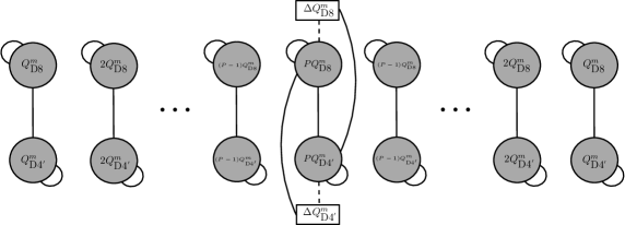
Figure 6: Completed quiver associated to the NATD solution.

The interpretation of the quiver quantum mechanics is as describing backreacted D0-D4 baryon vertices in the completely antisymmetric representation of the gauge groups U$(kQ_{\textrm{D8}}^{m})\times$U$(kQ_{\textrm{D4}^{\prime}}^{m})$ associated to a 5d intersection of D4’-D8 branes. The brane set-up associated to the quiver becomes after T+S duality, suitable Hanany-Witten moves and a further T-duality, the one depicted in Figure 7.

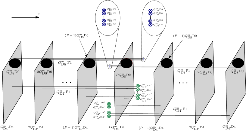
Figure 7: Brane set-up describing the baryon vertex interpretation of the quiver depicted in Figure 6.

One can check that, as expected, the holographic and field theory central charges, given by

$$c_{hol} = Q_{\text{D4}^{\prime}}^{m}Q_{\text{D8}}^{m}(4P^{3}-12P+8),$$ (63)

$$c_{ft} = Q_{\text{D4}^{\prime}}^{m}Q_{\text{D8}}^{m}(4P^{3}+2P),$$ (64)

coincide in the $P\rightarrow\infty$, holographic, limit.

Before we close this subsection we would like to report on recent progress in trying to connect the solution just discussed with the three dimensional black hole constructed in [47]. The aforementioned black hole was constructed by dualising the Principal Chiral Model with group manifold SL$(2,\mathbf{R})$ with respect to its whole isometry group, acting on the left. This is an AdS₃ geometry consisting on just metric which is not a good string theory background, since it does not satisfy the 10d equations of motion. Given that the same holds after dualisation, the black hole geometry constructed in [47] had limited applicability. In the remainder of this subsection we exploit the similarities between the construction carried out in [47] and the one pursued in this subsection to try to embed the black hole geometry of [47] in a valid string theory background. As we show this is not possible due to the sick behaviour of the dilaton.

Following [47] we can try to find a black hole geometry embedded in the non-Abelian T-dual solution given by (53) by writing it in terms of the Lagrange multipliers, $v_{i}$, and defining two different parametrisations for the regions $\nu^{2}>0$ and $\nu^{2}<0$, where $v^{2}=\eta^{ij}v_{i}v_{j}$ with $\eta^{ij}=(+,-,+)$. These two regions are interpreted as the interior and the exterior of the black hole construction in [47]. The solution (53) reads in terms of the Lagrange multipliers,

$$\begin{split}&ds^{2}=\frac{(dv_{1}^{2}-dv_{2}^{2}+dv_{3}^{2})-(v_{1}dv_{1}-v_{2}dv_{2}+v_{3}dv_{3})^{2}}{1-(v_{1}^{2}-v_{2}^{2}+v_{3}^{2})}+4ds^{2}_{\text{S}^{3}}+M^{2}ds^{2}_{\text{CY}_{2}},\\ &e^{-2\Phi}=(v_{1}^{2}-v_{2}^{2}+v_{3}^{2})-1,\qquad B_{2}=\frac{v_{3}dv_{1}\wedge dv_{2}-v_{2}dv_{1}\wedge dv_{3}+v_{1}dv_{2}\wedge dv_{3}}{(v_{1}^{2}-v_{2}^{2}+v_{3}^{2})-1},\\ &F_{0}=1,\qquad F_{2}=\frac{(v_{3}dv_{1}\wedge dv_{2}-v_{2}dv_{1}\wedge dv_{3}+v_{1}dv_{2}\wedge dv_{3})}{(v_{1}^{2}-v_{2}^{2}+v_{3}^{2})-1},\\ &F_{4}=-M^{4}\text{vol}_{\text{CY}_{2}}+8(v_{1}dv_{1}-v_{2}dv_{2}+v_{3}dv_{3})\wedge\text{vol}_{\text{S}^{3}}\,.\qquad\qquad\end{split}$$ (65)

Following [47] we then use the parametrisations

$$\begin{split}&v^{I}_{i}=(\sqrt{\rho}\cos\phi\cosh\xi,\sqrt{\rho}\sinh\xi,\sqrt{\rho}\sin\phi\cosh\xi),\\ &v^{II}_{i}=(\sqrt{\rho}\cos\phi\sinh\xi,\sqrt{\rho}\cosh\xi,\sqrt{\rho}\sin\phi\sinh\xi),\end{split}$$ (66)

in the two different regions

$$(v^{I})^{2}=\rho>0,\qquad\qquad(v^{II})^{2}=-\rho<0.$$ (67)

Note that both parametrisations in (66) are related under $\xi\to\xi-i\frac{\pi}{2}$ and $\rho\to-\rho$.

The geometry in region I reads,

$$\begin{split}&ds_{I}^{2}=\frac{\rho}{1-\rho}(-d\xi^{2}+\cosh^{2}\xi\;d\phi^{2})+\frac{d\rho^{2}}{4\rho}+M^{2}ds^{2}_{\text{CY}_{2}}+4ds^{2}_{\text{S}^{3}},\qquad e^{-2\Phi}=\rho-1,\\ &B_{2}=-\frac{\rho^{3/2}}{(\rho-1)}\cosh\xi\;d\phi\wedge d\xi,\qquad F_{0}=1,\qquad F_{2}=-\frac{\rho^{3/2}}{(\rho-1)}\cosh\xi\;d\phi\wedge d\xi,\\ &F_{4}=-M^{4}\text{vol}_{\text{CY}_{2}}+4\;d\rho\wedge\text{vol}_{\text{S}^{3}},\qquad\qquad\end{split}$$ (68)

while in region II it is given by

$$\begin{split}&ds_{II}^{2}=\frac{\rho}{\rho+1}(\sinh^{2}\xi\;d\tau^{2}+d\xi^{2})-\frac{d\rho^{2}}{4\rho}+M^{2}ds^{2}_{\text{CY}_{2}}+4L^{2}ds^{2}_{\text{S}^{3}}\;,\qquad e^{-2\Phi}=-(\rho+1)\;,\\ &B_{2}=-\frac{\rho^{3/2}}{\rho+1}\sinh\xi\;d\tau\wedge d\xi,\qquad F_{0}=1,\qquad F_{2}=-\frac{\rho^{3/2}}{\rho+1}\sinh\xi\;d\tau\wedge d\xi,\\ &F_{4}=-M^{4}\text{vol}_{\text{CY}_{2}}-4\;d\rho\wedge\text{vol}_{\text{S}^{3}}.\end{split}$$ (69)

In turn, the Ricci scalars in both regions read,

$$R_{I}=-\frac{\rho^{2}-6\rho+33}{2(\rho-1)^{2}},\qquad\qquad R_{II}=-\frac{\rho^{2}+6\rho+33}{2(\rho+1)^{2}}.$$ (70)

As for the black hole in [47] there is a singularity in region I at $\rho=1$, while the behaviour at $\rho=0$ is that of an event-horizon. This is reflected in the change of signature of the metric, going from (+,+,-,+,+,+,+,+,+,+) in region II to (+,-,+,+,+,+,+,+,+,+) in region I, and (-,+,+,+,+,+,+,+,+,+) beyond $\rho=1$. A detailed study of the causal structure associated to this geometry could now be carried out following [47]. Note however that there is a fundamental obstruction that invalidates a similar analysis to that in [47], since the dilaton is ill-defined both in region II (the would-be exterior of the black hole) and in region I when $\rho<1$ (the would-be interior of the black hole). This implies that the black hole constructed in [47] cannot be embedded within our supergravity background. The same conclusion is reached if one attempts to embed the black hole onto a more general solution in the class reviewed in section 2. In this case the Ricci scalar is singular when ${\tilde{\Delta}}$ vanishes, say at $\rho_{*}$. According to the interpretation in [47] $\rho\in[0,\rho_{*}]$ would parametrise the black hole interior, and $\rho<0$ the exterior, which is again where $\tilde{\Delta}<0$ and the dilaton is ill-defined.

3.3 Defect interpretation

In this subsection we show that it is possible to provide a defect interpretation to the solutions described in this section in complete analogy with the analysis performed in subsection 2.2. In this case the brane solutions whose near horizon geometries are the AdS${}_{2}\times S^{3}\times T^{4}\times I$ backgrounds were worked out in [40], and further analysed in [19], where they were interpreted in terms of D0-F1-D4 branes ending on D4’-D8 bound states. As in subsection 2.2 a parametrisation was obtained that allowed to relate a subclass of the AdS₂ geometries to a 6d domain wall solution to 6d $\mathcal{N}=(1,1)$ minimal gauged supergravity that asymptotes locally to AdS₆. This allowed to propose a dual interpretation of these AdS₂ solutions as line defect CFTs within the 5d Sp(N) CFT dual to the Brandhuber-Oz AdS₆ background.

As in the calculation in subsection 2.2, allowing the D4’-branes to be completely localised in their transverse space it is possible to recover a near-horizon geometry describing a D4’-D8 system wrapping an AdS${}_{2}\times S^{3}$ geometry, to which D0-F1-D4 branes need to be added to preserve supersymmetry [40]. The near-horizon reads

$$ds_{10}^{2}=H_{\textrm{D}4^{\prime}}^{-1/2}H_{\textrm{D}8}^{-1/2}\left[Q_{1}\left(ds_{\textrm{AdS}_{2}}^{2}+4ds_{S^{3}}^{2}\right)+H_{\textrm{D}4^{\prime}}H_{\textrm{D}8}dz^{2}+H_{\textrm{D}4^{\prime}}\,\left(d\rho^{2}+\rho^{2}\,ds_{\tilde{S}^{3}}^{2}\right)\right]\,,$$ (71)

with $Q_{1}$ a parameter related to the defect charges of D0-F1-D4 branes. One can check that this background is included in the classification reviewed in this section, for $\text{CY}_{2}=T^{4}$ locally and $u^{\prime}=0$.

As already mentioned, the previous brane intersection was linked to a 6d charged domain wall characterised by an AdS₂ slicing flowing asymptotically to the AdS₆ vacuum of 6d Romans supergravity. This domain wall is of the form

$$\begin{split}&ds^{2}_{6}=e^{2U(\mu)}\left(ds^{2}_{AdS_{2}}+4ds^{2}_{S^{3}}\right)+e^{2V(\mu)}d\mu^{2}\,,\\ &B_{2}=b(\mu)\,\text{vol}_{AdS_{2}}\,,\\ &X_{6}=X_{6}(\mu)\,,\end{split}$$ (72)

and, consistently with the whole picture, can be obtained through double analytical continuation from the domain wall solution in (LABEL:6dAdS3). The BPS equations for this background preserve 8 real supercharges and take the same form of (34) and (35). In analogy with the AdS₃ analysis, the 6d solution (LABEL:6dAdS2) reproduces locally in the limit $\mu\rightarrow 1$ the geometry of the AdS₆ vacuum, together with a singularity in the $\mu\rightarrow 0$ limit. Using the uplift formulas to massive IIA given in [19] one can check that the resulting domain wall solution in 10d is related to the near horizon geometry (71) through the change of coordinates [40]

$$z=\frac{3\,s^{2/3}\,e^{U}\,X_{6}}{\sqrt{2}\,g\,Q_{1}^{1/2}}\,,\qquad\rho=\frac{\sqrt{2}\,c\,e^{3U/2}}{g\,Q_{1}^{3/4}\,X_{6}^{1/2}}\,.$$ (73)

The AdS₂ solution is then specified by

$$H_{\mathrm{D}8}=\frac{s^{2/3}\,e^{U}\,X_{6}}{Q_{1}^{1/2}}\,,\qquad H_{\mathrm{D}4^{\prime}}=\frac{Q_{1}^{5/2}\,e^{-5U}}{\Sigma_{6}}\,,$$ (74)

with $h_{8}=H_{\mathrm{D}8}$ and $h_{4}=H_{\mathrm{D}4^{\prime}}$. These conditions are analogous to (42)-(43) for AdS₃, which is obviously related to the fact that the AdS₂ solutions and the AdS₃ backgrounds are related by double analytical continuation. In this case the solution is interpreted as a D0-F1-D4 line defect within the 5d Sp(N) fixed point theory.

4 Discussion

In these proceedings we have reviewed recent progress in the construction of AdS₃/CFT₂ and AdS₂/CFT₁ dual pairs in massive Type IIA string theory. These dual pairs represent new well-controlled string theory settings where the microscopical counting program of five and four dimensional black holes can be further developed. On a different note, our solutions allow for a defect interpretation in terms of surface or line defects within the 5d Sp(N) fixed point theory. In general grounds having at our disposal the holographic description of these defect CFTs allows to apply holographic methods to the computation of central charges, correlators and other observables of the defect CFT.

Notably, other AdS/CFT pairs have been constructed in the recent literature that can also be taken as set-ups where to carry out the microscopical counting program of black holes as well as the holographic study of defect CFTs. The most direct extensions of the solutions here presented are the $\text{AdS}_{3}\times S^{2}\times M_{4}\times I$ and $\text{AdS}_{2}\times S^{3}\times M_{4}\times I$ solutions to massive IIA supergravity with $M_{4}$ a Kähler manifold, constructed in [1, 18, 2]. These solutions have been left out of our analysis because the corresponding field theory duals have only been partially explored or not explored at all. In the $\text{AdS}_{3}$ case, when $I=S^{1}$ and there are no D4-branes present, these solutions are related to the class discussed in [4] via Abelian T-duality. Therefore, the dual CFTs are described in terms of D3-branes wrapping complex curves in elliptically fibrered $\text{CY}_{3}$ manifolds. More general field theory settings related to these solutions have not yet been explored, neither have their possible realisations as defects within higher dimensional CFTs. These constitute interesting new research avenues to explore.

In [18] $\text{AdS}_{3}\times S^{3}\times M_{4}\times I$ solutions to M-theory where $M_{4}$ is either a $\text{CY}_{2}$ or a Kähler manifold have been constructed. These solutions preserve the same number of supersymmetries as the solutions here presented, and for $M_{4}=\text{CY}_{2}$ are dual to quiver CFTs similar to the ones reviewed in subsection 2.1, which in this case describe M-strings (see [79, 80]). In [19] it was shown that a subset of these solutions can be interpreted as surface defects within 6d (1,0) CFTs living in M5-branes probing ALE singularities. Moreover, upon reduction these solutions give rise to a new class of $\text{AdS}_{3}\times S^{3}\times S^{2}\times\Sigma_{2}$ solutions, with $\Sigma_{2}$ a 2d Riemann surface, that can be interpreted as defects within the 6d (1,0) CFT dual to the AdS₇ solution to massless Type IIA supergravity. The description of the dual 2d CFT in terms of quivers embedded in the 6d quiver associated to the D6-NS5 intersection was also worked out in [19]. Similarly, new classes of $\text{AdS}_{3}\times S^{2}\times S^{2}\times S^{1}\times\Sigma_{2}$ solutions with the same number of supersymmetries have been constructed in Type IIB supergravity [21], some of which admit a defect interpretation within the 5d Sp(N) fixed point theory (this time realised in a Type IIB brane intersection) and/or describe holographic duals of D3-brane boxes, as the ones discussed in [81]. The readers are referred to [21] for the details of these constructions. More recently, the parallel in Type IIB of the general classification of AdS₃ spaces with $\mathcal{N}=(0,4)$ supersymmetries in [1] has been carried out in [82]. The readers can again find the details of these constructions in the original reference. An interesting open line to explore is the construction of the 2d CFTs dual to these solutions, along the lines of [11, 12, 26].

Similarly, new classes of AdS₂ solutions in Type IIB with 4 supersymmetries have been constructed in [20], acting with Abelian T-duality on the AdS₃ subspace of the solutions reviewed in section 2. These solutions are dual, by construction [43, 44], to SCQMs realised as discrete light-cone compactifications of the 2d dual CFTs reviewed in this paper. Further solutions of the type $\text{AdS}_{2}\times S^{2}\times\text{CY}_{2}\times\Sigma_{2}$ with $\Sigma_{2}$ an annulus have been constructed in [22], via Abelian T-duality acting on the AdS₂ solutions reviewed in section 3. The SCQMs dual to these solutions are thus the same as the ones reviewed in that section, and allow for a similar defect interpretation, this time as backreacted D1-D3 baryon vertices within the 5d Sp(N) fixed point theory, now realised on a D5-NS5-D7 brane web. More recently, new classes of AdS₂ solutions with the same number of supersymmetries have been constructed in both Type IIA and Type IIB supergravities that allow a description in terms of backreacted baryon vertices within 4d $\mathcal{N}=4$ SYM or orbifolds thereof. In this case the solutions are asymptotically locally $\text{AdS}_{5}\times S^{5}/\mathbb{Z}_{k}$ (or its Abelian T-dual in the IIA case). The reader is referred to [24] for more details on these constructions.

An obviously interesting avenue to pursue is to investigate the CFT duals to the broader class of AdS₃ solutions constructed in [1] for which there is a dependence on the internal structure of the $\text{CY}_{2}$ manifold. This would allow to extend the 2d and 1d CFTs discussed in this paper by further exploiting the interplay between string theory dualities and the AdS/CFT correspondence, as described in the previous paragraphs. We expect to report progress in these directions in the near future.

Acknowledgements

We would like to thank Chris Couzens, Federico Faedo, Niall Macpherson, Carlos Nunez, Stefano Speziali and Stefan Vandoren for collaboration in some of the results reviewed in these proceedings. YL and AR are partially supported by the Spanish government grant PGC2018-096894-B-100. AR is partially supported by the Heising-Simons Foundation, the Simons Foundation, and the National Science Foundation Grant No. NSF PHY-1748958. The work of NP is supported by the Israel Science Foundation (grant No. 741/20) and by the German Research Foundation through a German-Israeli Project Cooperation (DIP) grant "Holography and the Swampland".

References

- [1] Y. Lozano, N. T. Macpherson, C. Nunez and A. Ramirez, “AdS3 solutions in Massive IIA with small supersymmetry,” JHEP 01, 129 (2020) [arXiv:1908.09851 [hep-th]].
- [2] Y. Lozano, C. Nunez, A. Ramirez and S. Speziali, “AdS2 duals to ADHM quivers with Wilson lines,” JHEP 03 (2021), 145 [arXiv:2011.13932 [hep-th]].
- [3] D. Tong, “The holographic dual of ,” JHEP 04 (2014), 193 [arXiv:1402.5135 [hep-th]].
- [4] C. Couzens, C. Lawrie, D. Martelli, S. Schafer-Nameki and J. M. Wong, “F-theory and AdS3/CFT2,” JHEP 1708, 043 (2017) [arXiv:1705.04679 [hep-th]].
- [5] L. Eberhardt, M. R. Gaberdiel and W. Li, “A holographic dual for string theory on AdSSSS1,” JHEP 08 (2017), 111 [arXiv:1707.02705 [hep-th]].
- [6] S. Datta, L. Eberhardt and M. R. Gaberdiel, “Stringy holography for AdS3,” JHEP 01 (2018), 146 [arXiv:1709.06393 [hep-th]].
- [7] C. Couzens, D. Martelli and S. Schafer-Nameki, “F-theory and AdS3/CFT2 (2, 0),” JHEP 1806 (2018) 008 [arXiv:1712.07631 [hep-th]].
- [8] M. R. Gaberdiel and R. Gopakumar, “Tensionless string spectra on AdS3,” JHEP 05 (2018), 085 [arXiv:1803.04423 [hep-th]].
- [9] L. Eberhardt and I. G. Zadeh, “ holography on ,” JHEP 07 (2018), 143 [arXiv:1805.09832 [hep-th]].
- [10] L. Eberhardt, M. R. Gaberdiel and R. Gopakumar, “The Worldsheet Dual of the Symmetric Product CFT,” JHEP 04 (2019), 103 [arXiv:1812.01007 [hep-th]].
- [11] Y. Lozano, N. T. Macpherson, C. Nunez and A. Ramirez, “1/4 BPS solutions and the AdS3/CFT2 correspondence,” Phys. Rev. D 101, no.2, 026014 (2020) [arXiv:1909.09636 [hep-th]].
- [12] Y. Lozano, N. T. Macpherson, C. Nunez and A. Ramirez, “Two dimensional quivers dual to AdS3 solutions in massive IIA,” JHEP 01, 140 (2020) [arXiv:1909.10510 [hep-th]].
- [13] Y. Lozano, N. T. Macpherson, C. Nunez and A. Ramirez, “AdS3 solutions in massive IIA, defect CFTs and T-duality,” JHEP 12, 013 (2019) [arXiv:1909.11669 [hep-th]].
- [14] L. Eberhardt, M. R. Gaberdiel and R. Gopakumar, “Deriving the AdS3/CFT2 correspondence,” JHEP 02 (2020), 136 [arXiv:1911.00378 [hep-th]].
- [15] C. Couzens, “ = (0, 2) AdS3 solutions of type IIB and F-theory with generic fluxes,” JHEP 04 (2021), 038 [arXiv:1911.04439 [hep-th]].
- [16] C. Couzens, H. het Lam and K. Mayer, “Twisted = 1 SCFTs and their AdS3 duals,” JHEP 03 (2020), 032 [arXiv:1912.07605 [hep-th]].
- [17] G. Dibitetto, Y. Lozano, N. Petri and A. Ramirez, “Holographic description of M-branes via AdS2,” JHEP 04 (2020), 037 [arXiv:1912.09932 [hep-th]].
- [18] Y. Lozano, C. Nunez, A. Ramirez and S. Speziali, “-strings and AdS3 solutions to M-theory with small supersymmetry,” JHEP 08 (2020), 118 [arXiv:2005.06561 [hep-th]].
- [19] F. Faedo, Y. Lozano and N. Petri, “Searching for surface defect CFTs within AdS3,” JHEP 11 (2020), 052 [arXiv:2007.16167 [hep-th]].
- [20] Y. Lozano, C. Nunez, A. Ramirez and S. Speziali, “New AdS2 backgrounds and = 4 conformal quantum mechanics,” JHEP 03 (2021), 277 [arXiv:2011.00005 [hep-th]].
- [21] F. Faedo, Y. Lozano and N. Petri, “New AdS3 near-horizons in Type IIB,” JHEP 04 (2021), 028 [arXiv:2012.07148 [hep-th]].
- [22] Y. Lozano, C. Nunez and A. Ramirez, “ solutions in Type IIB with 8 supersymmetries,” JHEP 04 (2021), 110 [arXiv:2101.04682 [hep-th]].
- [23] A. Ramirez, “AdS2 geometries and non-Abelian T-duality in non-compact spaces,” JHEP 10 (2021), 020 [arXiv:2106.09735 [hep-th]].
- [24] Y. Lozano, N. Petri and C. Risco, “New AdS2 supergravity duals of 4d SCFTs with defects,” JHEP 10 (2021), 217 [arXiv:2107.12277 [hep-th]].
- [25] C. Couzens, N. T. Macpherson and A. Passias, “ = (2, 2) AdS3 from D3-branes wrapped on Riemann surfaces,” JHEP 02 (2022), 189 [arXiv:2107.13562 [hep-th]].
- [26] C. Couzens, Y. Lozano, N. Petri and S. Vandoren, “ Black String Chains,” [arXiv:2109.10413 [hep-th]].
- [27] R. Argurio, A. Giveon and A. Shomer, “Superstring theory on AdS(3) x G / H and boundary N=3 superconformal symmetry,” JHEP 0004, 010 (2000) [hep-th/0002104].
- [28] A. Karch and L. Randall, “Open and closed string interpretation of SUSY CFT’s on branes with boundaries,” JHEP 06 (2001), 063 [arXiv:hep-th/0105132 [hep-th]].
- [29] O. DeWolfe, D. Z. Freedman and H. Ooguri, “Holography and defect conformal field theories,” Phys. Rev. D 66 (2002), 025009 [arXiv:hep-th/0111135 [hep-th]].
- [30] O. Aharony, O. DeWolfe, D. Z. Freedman and A. Karch, “Defect conformal field theory and locally localized gravity,” JHEP 07 (2003), 030 [arXiv:hep-th/0303249 [hep-th]].
- [31] E. D’Hoker, J. Estes and M. Gutperle, “Ten-dimensional supersymmetric Janus solutions,” Nucl. Phys. B 757 (2006), 79-116 [arXiv:hep-th/0603012 [hep-th]].
- [32] O. Lunin, “1/2-BPS states in M theory and defects in the dual CFTs,” JHEP 10 (2007), 014 [arXiv:0704.3442 [hep-th]].
- [33] E. D’Hoker, J. Estes and M. Gutperle, “Exact half-BPS Type IIB interface solutions. I. Local solution and supersymmetric Janus,” JHEP 06 (2007), 021 [arXiv:0705.0022 [hep-th]].
- [34] E. D’Hoker, J. Estes and M. Gutperle, “Gravity duals of half-BPS Wilson loops,” JHEP 0706, 063 (2007) [arXiv:0705.1004 [hep-th]].
- [35] M. Chiodaroli, M. Gutperle and D. Krym, “Half-BPS Solutions locally asymptotic to AdS(3) x S**3 and interface conformal field theories,” JHEP 02, 066 (2010) [arXiv:0910.0466 [hep-th]].
- [36] M. Chiodaroli, E. D’Hoker and M. Gutperle, “Open Worldsheets for Holographic Interfaces,” JHEP 03, 060 (2010) [arXiv:0912.4679 [hep-th]].
- [37] G. Dibitetto and N. Petri, “BPS objects in D = 7 supergravity and their M-theory origin,” JHEP 1712, 041 (2017) [arXiv:1707.06152 [hep-th]].
- [38] G. Dibitetto and N. Petri, “6d surface defects from massive type IIA,” JHEP 1801, 039 (2018) [arXiv:1707.06154 [hep-th]].
- [39] G. Dibitetto and N. Petri, “Surface defects in the D4 D8 brane system,” JHEP 1901, 193 (2019) [arXiv:1807.07768 [hep-th]].
- [40] G. Dibitetto and N. Petri, “AdS2 solutions and their massive IIA origin,” JHEP 1905, 107 (2019) [arXiv:1811.11572 [hep-th]].
- [41] K. Chen, M. Gutperle and M. Vicino, “Holographic Line Defects in , Gauged Supergravity,” Phys. Rev. D 102 (2020) no.2, 026025 [arXiv:2005.03046 [hep-th]].
- [42] M. Gutperle and C. F. Uhlemann, “Surface defects in holographic 5d SCFTs,” JHEP 04 (2021), 134 [arXiv:2012.14547 [hep-th]].
- [43] V. Balasubramanian, A. Naqvi and J. Simon, “A Multiboundary AdS orbifold and DLCQ holography: A Universal holographic description of extremal black hole horizons,” JHEP 08 (2004), 023 [arXiv:hep-th/0311237 [hep-th]].
- [44] V. Balasubramanian, J. de Boer, M. Sheikh-Jabbari and J. Simon, “What is a chiral 2d CFT? And what does it have to do with extremal black holes?,” JHEP 02, 017 (2010) [arXiv:0906.3272 [hep-th]].
- [45] N. Seiberg, “Five-dimensional SUSY field theories, nontrivial fixed points and string dynamics,” Phys. Lett. B 388 (1996), 753-760 [arXiv:hep-th/9608111 [hep-th]].
- [46] A. Brandhuber and Y. Oz, “The D-4 - D-8 brane system and five-dimensional fixed points,” Phys. Lett. B 460 (1999), 307-312 [arXiv:hep-th/9905148 [hep-th]].
- [47] E. Alvarez, L. Alvarez-Gaume, J. L. F. Barbon and Y. Lozano, “Some global aspects of duality in string theory,” Nucl. Phys. B 415 (1994), 71-100 [arXiv:hep-th/9309039 [hep-th]].
- [48] G. Dibitetto and N. Petri, “AdS3 from M-branes at conical singularities,” JHEP 01 (2021), 129 [arXiv:2010.12323 [hep-th]].
- [49] Y. Imamura, “1/4 BPS solutions in massive IIA supergravity,” Prog. Theor. Phys. 106 (2001), 653-670 [arXiv:hep-th/0105263 [hep-th]].
- [50] H. C. Kim, “Line defects and 5d instanton partition functions,” JHEP 03 (2016), 199 [arXiv:1601.06841 [hep-th]].
- [51] B. Assel and A. Sciarappa, “Wilson loops in 5d theories and S-duality,” JHEP 10 (2018), 082 [arXiv:1806.09636 [hep-th]].
- [52] B. Assel and A. Sciarappa, “On monopole bubbling contributions to ’t Hooft loops,” JHEP 05 (2019), 180 [arXiv:1903.00376 [hep-th]].
- [53] D. Tong and K. Wong, “Instantons, Wilson lines, and D-branes,” Phys. Rev. D 91 (2015) no.2, 026007 [arXiv:1410.8523 [hep-th]].
- [54] C. M. Chang, O. Ganor and J. Oh, “An index for ray operators in 5d SCFTs,” JHEP 02 (2017), 018 [arXiv:1608.06284 [hep-th]].
- [55] S. Yamaguchi, “Wilson loops of anti-symmetric representation and D5-branes,” JHEP 05 (2006), 037 [arXiv:hep-th/0603208 [hep-th]].
- [56] J. Gomis and F. Passerini, “Wilson Loops as D3-Branes,” JHEP 01 (2007), 097 [arXiv:hep-th/0612022 [hep-th]].
- [57] E. Witten, “Baryons and branes in anti-de Sitter space,” JHEP 07, 006 (1998) [arXiv:hep-th/9805112 [hep-th]].
- [58] F. Denef, “Quantum quivers and Hall / hole halos,” JHEP 10 (2002), 023 [arXiv:hep-th/0206072 [hep-th]].
- [59] K. Sfetsos and D. C. Thompson, “On non-abelian T-dual geometries with Ramond fluxes,” Nucl. Phys. B 846 (2011), 21-42 [arXiv:1012.1320 [hep-th]].
- [60] Y. Lozano, E. O Colgain, K. Sfetsos and D. C. Thompson, “Non-abelian T-duality, Ramond Fields and Coset Geometries,” JHEP 06 (2011), 106 [arXiv:1104.5196 [hep-th]].
- [61] G. Itsios, Y. Lozano, E. O Colgain and K. Sfetsos, “Non-Abelian T-duality and consistent truncations in type-II supergravity,” JHEP 08 (2012), 132 [arXiv:1205.2274 [hep-th]].
- [62] Y. Lozano, E. Ó Colgáin, D. Rodríguez-Gómez and K. Sfetsos, “Supersymmetric via T Duality,” Phys. Rev. Lett. 110 (2013) no.23, 231601 [arXiv:1212.1043 [hep-th]].
- [63] G. Itsios, C. Nunez, K. Sfetsos and D. C. Thompson, “Non-Abelian T-duality and the AdS/CFT correspondence:new N=1 backgrounds,” Nucl. Phys. B 873 (2013), 1-64 [arXiv:1301.6755 [hep-th]].
- [64] G. Itsios, C. Nunez, K. Sfetsos and D. C. Thompson, “On Non-Abelian T-Duality and new N=1 backgrounds,” Phys. Lett. B 721 (2013), 342-346 [arXiv:1212.4840 [hep-th]].
- [65] Y. Lozano and N. T. Macpherson, “A new AdS4/CFT3 dual with extended SUSY and a spectral flow,” JHEP 11 (2014), 115 [arXiv:1408.0912 [hep-th]].
- [66] K. Sfetsos and D. C. Thompson, “New supersymmetric backgrounds in Type IIA supergravity,” JHEP 11 (2014), 006 [arXiv:1408.6545 [hep-th]].
- [67] Ö. Kelekci, Y. Lozano, N. T. Macpherson and E. Ó. Colgáin, “Supersymmetry and non-Abelian T-duality in type II supergravity,” Class. Quant. Grav. 32 (2015) no.3, 035014 [arXiv:1409.7406 [hep-th]].
- [68] N. T. Macpherson, C. Núñez, L. A. Pando Zayas, V. G. J. Rodgers and C. A. Whiting, “Type IIB supergravity solutions with AdS5 from Abelian and non-Abelian T dualities,” JHEP 02 (2015), 040 [arXiv:1410.2650 [hep-th]].
- [69] Y. Bea, J. D. Edelstein, G. Itsios, K. S. Kooner, C. Nunez, D. Schofield and J. A. Sierra-Garcia, “Compactifications of the Klebanov-Witten CFT and new AdS3 backgrounds,” JHEP 05 (2015), 062 [arXiv:1503.07527 [hep-th]].
- [70] Y. Lozano, N. T. Macpherson, J. Montero and E. Ó. Colgáin, “New T-duals with supersymmetry,” JHEP 08 (2015), 121 [arXiv:1507.02659 [hep-th]].
- [71] Y. Lozano, N. T. Macpherson and J. Montero, “A supersymmetric AdS4 solution in M-theory with purely magnetic flux,” JHEP 10 (2015), 004 [arXiv:1507.02660 [hep-th]].
- [72] N. T. Macpherson, C. Nunez, D. C. Thompson and S. Zacarias, “Holographic Flows in non-Abelian T-dual Geometries,” JHEP 11 (2015), 212 [arXiv:1509.04286 [hep-th]].
- [73] L. A. Pando Zayas, V. G. J. Rodgers and C. A. Whiting, “Supergravity solutions with AdS4 from non-Abelian T-dualities,” JHEP 02 (2016), 061 [arXiv:1511.05991 [hep-th]].
- [74] Y. Lozano and C. Núñez, “Field theory aspects of non-Abelian T-duality and 2 linear quivers,” JHEP 05 (2016), 107 [arXiv:1603.04440 [hep-th]].
- [75] Y. Lozano, N. T. Macpherson, J. Montero and C. Nunez, “Three-dimensional linear quivers and non-Abelian T-duals,” JHEP 11 (2016), 133 [arXiv:1609.09061 [hep-th]].
- [76] Y. Lozano, C. Nunez and S. Zacarias, “BMN Vacua, Superstars and Non-Abelian T-duality,” JHEP 09 (2017), 008 [arXiv:1703.00417 [hep-th]].
- [77] G. Itsios, Y. Lozano, J. Montero and C. Nunez, “The AdS5 non-Abelian T-dual of Klebanov-Witten as a linear quiver from M5-branes,” JHEP 09 (2017), 038 [arXiv:1705.09661 [hep-th]].
- [78] X. C. de la Ossa and F. Quevedo, “Duality symmetries from nonAbelian isometries in string theory,” Nucl. Phys. B 403 (1993), 377-394 [arXiv:hep-th/9210021 [hep-th]].
- [79] B. Haghighat, C. Kozcaz, G. Lockhart and C. Vafa, “Orbifolds of M-strings,” Phys. Rev. D 89 (2014) no.4, 046003 [arXiv:1310.1185 [hep-th]].
- [80] A. Gadde, B. Haghighat, J. Kim, S. Kim, G. Lockhart and C. Vafa, “6d String Chains,” JHEP 02 (2018), 143 [arXiv:1504.04614 [hep-th]].
- [81] A. Hanany and T. Okazaki, “(0,4) brane box models,” JHEP 03 (2019), 027 [arXiv:1811.09117 [hep-th]].
- [82] N. T. Macpherson and A. Ramirez, “AdS S2 in IIB with small supersymmetry,” [arXiv:2202.00352 [hep-th]].