Efficient Reconstruction of Stochastic Pedigrees:
Some Steps From Theory to Practice

Abstract

In an extant population, how much information do extant individuals provide on the pedigree of their ancestors? Recent work by Kim, Mossel, Ramnarayan and Turner (2020) studied this question under a number of simplifying assumptions, including random mating, fixed length inheritance blocks and sufficiently large founding population. They showed that under these conditions if the average number of offspring is a sufficiently large constant, then it is possible to recover a large fraction of the pedigree structure and genetic content by an algorithm they named REC-GEN.

We are interested in studying the performance of REC-GEN on simulated data generated according to the model. As a first step, we improve the running time of the algorithm. However, we observe that even the faster version of the algorithm does not do well in any simulations in recovering the pedigree beyond 2 generations. We claim that this is due to the inbreeding present in any setting where the algorithm can be run, even on simulated data. To support the claim we show that a main step of the algorithm, called ancestral reconstruction, performs accurately in an idealized setting with no inbreeding but performs poorly in random mating populations.

To overcome the poor behavior of REC-GEN we introduce a Belief-Propagation based heuristic that accounts for the inbreeding and performs much better in our simulations.

Preprint of an article published in Pacific Symposium on Biocomputing © 2022 World Scientific Publishing Co., Singapore, http://psb.stanford.edu/

1 Introduction

We follow up on a recent work by Kim et al [1]., the main motivation of which is to understand how much kinship information can be learned from DNA. More concretely, Kim et al. study the inference problem of recovering ancestral kinship relationships of a population of extant (present-day) individuals using only their genetic data for a mathematical generative model of pedigrees and DNA sequences on them based on the combinatorial framework of Steel and Hein[2] and Thatte and Steel[3], who also proved a rigorous statement about recovery of idealized pedigree models. The goal is to use this extant genetic data to recover the pedigree of the extant population under this model.

To study this question, Ref. 1 introduces an idealized model for generating pedigree data. The population model they use is a standard random mating model, but the genetic inheritance model assumes that inheritance blocks are of fixed length. This removes the additional difficulty of “phasing” which allows for a rigorous analysis.

The main contribution of Ref. 1 is to show that under certain conditions, the algorithm proposed in the paper, named Rec-Gen, approximately recovers the true, unknown pedigree as well as its genetic content. There is a huge body of work on pedigree reconstruction, see e.g. Ref. 4, 5, 6, 7, 8, 9, 10, 11. In contrast to Ref. 1, most of this work does not provide theoretical guarantees. In this paper we take the theoretical analysis in Ref. 1 and study to what extent it can be applied in more realistic settings.

There is a tension between different aspects of the assumptions in Ref. 1. On one hand, they require a very big pedigree to avoid inbreeding. On the other, the algorithm Rec-Gen has cubic running time. While in the limit as the pedigree size goes to infinity, this tension disappears, we find that applying the algorithm on simulated data results either in poor accuracy or an infeasible running time.

Our main contributions in this paper are:

• We improve the algorithm runtime to essentially quadratic for model-generated data.

• We then observe that even the faster version of the algorithm does not do well in any simulations in recovering the pedigree beyond 2 generations.

• We claim that this is due to the inbreeding present in any setting where the algorithm can be run, even on simulated data.

• To support the claim we show that a main step of the algorithm, called ancestral reconstruction, performs accurately in a setting with no inbreeding but performs poorly in random mating populations.

• Finally, to overcome the poor behavior of REC-GEN we introduce a Belief-Propagation based heuristic that accounts for the inbreeding and performs much better in our simulations.

2 Model Description

We model populations as in Ref. 1. Here, we briefly restate the definition of a coupled pedigree, the structure manipulated by the Rec-Gen algorithm and introduce notation relevant to the description of our modified algorithm.

A $(N,B,T,\xi)$-uncoupled pedigree $\mathcal{U}$ is a directed acyclic graph $(V,E)$ in which vertices $v\in V$ represent individuals and edges $e=(u,v)\in E$ represent the relationship that $u$ is a parent of $v$. The set of vertices $V$ can be partitioned into $T+1$ subsets $V_{0},\dots,V_{T}$ so that each $v\in V_{i}$, $0\leq i<T$ has exactly two in-edges, both of which are from vertices in $V_{i+1}$. The sets $V_{i}$ represent generations, where $V_{0}$ is the extant population and $V_{T}$ is the founding population. The size of the founding population $|V_{T}|$ equals $N$. The vertices $V$ also satisfy monogamy — within each generation $V_{i}$, $i>0$, the vertices $V_{i}$ can be partitioned into pairs $(v_{1},v_{2})$ such that if $u$ is a child of $v_{1}$ if and only if $u$ is a child of $v_{2}$; such pairs are called couples. The number of children of each couple is randomly drawn from the distribution $\xi$.

Each vertex $v$ has associated genetic information in the form of $B$ blocks, each of which contains a symbol sampled from some alphabet $\Sigma$. The symbol at block $b$ of the genome of vertex $v$ is denoted $s_{v}(b)$.

The $(N,B,T,\xi)$-coupled pedigree $\mathcal{P}$ induced by an uncoupled pedigree $\mathcal{U}$ is formed by merging each couple into a single vertex — the resulting vertices are called coupled nodes. Now each $v$ in a generation other than the extant represents a pair of individuals, and an edge from a coupled node $u$ to a coupled node $v$ represents that $u$ is the parent of one of the individuals in couple $u$. All vertices in $\mathcal{P}$ have in-degree two, except vertices in the extant population, which remain uncoupled and have in-degree 1. The genetic information $s_{v}(b)$ of a coupled node $v$ is the set of all symbols that are in block $b$ for some individual in the couple represented by $v$.

When we say that some graph is a pedigree in this paper without specifying whether the pedigree is coupled or uncoupled, we are referencing coupled pedigrees.

3 Rec-Gen

The Rec-Gen reconstruction algorithm presented in Ref. 1 proceeds in three main phases. In each generation, siblinghood detection reconstructs relationships in the current generation, outputting a siblinghood hypergraph in which triple $u,v,w$ forms a hyperedge if they are likely to be siblings. Parent construction processes maximal cliques in the outputted hypergraph, populating the parent generation. Symbol collection reconstructs the genetic information of the parent generation.

3.1 Runtime Analysis

Naïve implementations of siblinghood detection and symbol collection both run in $\Omega(BN_{0}^{3})$ time. The siblinghood test counts the number of shared blocks in all triples, which can require $\Omega(BN_{0}^{3})$ in the worst case.

To naïvely find a triple of extant vertices sharing a gene in block $b$ with $u$ as their joint-LCA for some $u$ in generation $t$ of the pedigree for symbol collection it may be necessary to inspect all triples of extant descendants of $u$ in each block $b$, which is also $\Omega(BN_{0}^{3})$.

We wish to improve both of these processes to $O(BN_{0}^{2})$, as described in Sections 3.2 and 3.3.

3.2 Faster Siblinghood Detection

The greatest bottleneck in the runtime of Rec-Gen is the siblinghood detection step, which for each generation $t$ is cubic in the size of that generation $N_{t}$. To reduce the runtime from $O\left(N_{t}^{3}B\right)$ to $O\left(N_{t}^{2}B\right)$, we begin by processing all pairs of vertices, marking pairs that share some threshold $\theta=0.4$ of their blocks as sibling candidates. We then only consider triples of vertices formed from sibling candidates when generating the siblinghood hypergraph. Pseudocode of the alternate algorithm Perform statistical tests to detect siblinghood follows:

Algorithm 1 Perform statistical tests to detect siblinghood

Fast-Test-Siblinghood

1:procedure Fast-Test-Siblinghood(depth $(k-1)$ pedigree $\hat{\mathcal{P}}$)

2:     $C\leftarrow\varnothing$

3:     $V\leftarrow$ vertices of $\hat{\mathcal{P}}$ at level $k-1$

4:     for all distinct pairs $\{u,v\}\in 2^{V}$ do

5:         if  $\geq 0.4|B|$ blocks $b$ such that $\hat{s}_{u}(b)\cap\hat{s}_{v}(b)\neq\varnothing$  then

6:              $C\leftarrow C\cup\{u,v\}$               

7:     $E\leftarrow\varnothing$

8:     for all pairs $\{u,v\}\in C$ do

9:         for all  $w\in V$ at level $k-1$ such that $w\neq u\land w\neq v$  do

10:              if  $\geq 0.21|B|$ blocks $b$ such that $\hat{s}_{u}(b)\cap\hat{s}_{v}(b)\cap\hat{s}_{w}(b)\neq\varnothing$  then

11:                  $E\leftarrow E\cup\{u,v,w\}$                             

12:     $\hat{G}\leftarrow(V,E)$

13:     return $\hat{G}$

3.3 Faster Symbol Collection

To decrease the complexity of executing the Rec-Gen symbol-collection phase on $v$, we avoid explicitly searching for extant triples that have $v$ as their joint-LCA. Instead, we make the simplifying assumption that any three extant vertices $x,y,z$ descended from distinct children of $v$ have $v$ as a joint-LCA. Now, we can use the following modified algorithm to achieve an effect equivalent to the original symbol collection of Ref. 1:

• Let $\hat{G}_{u}(b)$ for a child $u$ of $v$ and block $b$ be the set of genes $g$ such that there exists an extant descendant $x$ of $u$ such that $\hat{s}_{u}(b)=\{g\}$.

• Compute $\hat{G}_{u}(b)$ for all children $u$ of $v$.

• Let $\hat{s}_{v}(b)$ be the two genes that are present in the greatest number of computed sets $\hat{G}_{u}(b)$.

Pseudocode of this modified process can be seen in Algorithm Empirically reconstruct the symbols of top-level node $v$ in $\mathcal{P}$..

Ref. 1 prove that, conditioned on the nonoccurence of undesirable inbreeding events, the existence of a joint-LCA $v$ for three nodes $x,y,z$ entails that $v$ is their unique LCA. Therefore, if most extant nodes have a joint-LCA, then the algorithm described above is equivalent to the initial description of symbol-collection. Empirically, very few ($<1\%$ of) extant triples in simulated pedigrees are descended from unique children of a vertex that is not their joint-LCA.

Generating $\hat{G}_{u}$ requires time that is linear in the number of nodes in the descendants pedigree of $u$. Since $\alpha>2$, this is on expectation bounded above by a linear function of the number of extant descendants of $u$. Each extant individual $v$ has at most $2^{t}$ ancestors in generation $t$. Therefore, the sum of the number of extant descendants of $u$ over all $u$ in generation $t$ is at most $2^{t}N_{0}$, where $N_{0}$ is the size of the extant population, so that the runtime of invoking Algorithm Empirically reconstruct the symbols of top-level node $v$ in $\mathcal{P}$. for all $u$ at generation $t$ is $O(B\cdot(2^{t}N_{0}+|G|))$. Since $\alpha>2$, $2^{t}\subseteq O(\alpha^{t})\subseteq O(\mathbb{E}[N_{t}]/N_{T})$, so that the total runtime of Algorithm Empirically reconstruct the symbols of top-level node $v$ in $\mathcal{P}$. is $O(B\cdot\mathbb{E}[N_{t}]N_{0}/N_{T})\subseteq O(BN_{0}^{2})$.

Algorithm 2 Empirically reconstruct the symbols of top-level node $v$ in $\mathcal{P}$.

Fast Collect-Symbols

1:procedure Fast Collect-Symbols($v,\hat{\mathcal{P}}$)

2:     for all blocks $b\in[B]$ do

3:         $c_{g}\leftarrow 0\;\forall\;g$

4:         for all children $u$ of $v$ do

5:              $\hat{G}_{u}(b)\leftarrow\varnothing$

6:              for all extant $x$ descended from $u$ do

7:                  $\hat{G}_{u}(b)\leftarrow\hat{G}_{u}(b)\cup\hat{s}_{x}(b)$               

8:              for all $g\in\hat{G}_{u}(b)$ do

9:                  $c_{g}\leftarrow c_{g}+1$                        

10:         $\sigma_{1}\leftarrow g\text{ with highest }c_{g}$

11:         $\sigma_{2}\leftarrow g\text{ with second-highest }c_{g}$

12:         Record the symbols $\sigma_{1},\sigma_{2}$ for block $b$ in $v$.      

4 Simulations

We assess the empirical accuracy of Rec-Gen and other algorithms presented later in this work by running them on simulated pedigrees. We generate pedigrees satisfying the stochastic model, as described in section 4.1. The extant populations of the pedigrees can be used as input for our implementations of the reconstructive algorithms, and a grader program evaluates the accuracy of the result as described in section 4.2.

4.1 Generating Pedigrees

For a given $\alpha$, our pedigree generator program creates $(N,B,T,\xi)$-coupled pedigrees according to the breeding and inheritance behaviors described in Section 2, where $\xi$ is either Poisson-distributed with parameter $\alpha$ or a constant distribution, $\xi=\alpha$.

4.2 Assessing Reconstruction Accuracy

Our grader program takes as input a parameter $\alpha\in[0,1)$ and two pedigrees with identical extant populations and the same numbers of generations — an original pedigree $\mathcal{P}$ and its reconstruction $\mathcal{P}^{\prime}$. It outputs a partial mapping between the coupled nodes of $\mathcal{P}$ and $\mathcal{P}^{\prime}$, where a coupled node $v\in\mathcal{P}$ of the original pedigree is mapped to a coupled node $v^{\prime}\in\mathcal{P}^{\prime}$ of the reconstructed pedigree only if $v^{\prime}$ is an $\alpha$-successful reconstruction of $v$. $\alpha$-successful reconstructions are defined recursively in the following manner:

• In generation 0 (the extant population) a vertex $v^{\prime}\in\mathcal{P}^{\prime}$ is an $\alpha$-successful reconstruction of $v\in\mathcal{P}$ if and only if $v$ and $v^{\prime}$ are the same coupled node.

• In generation $t>0$, let $c(v,v^{\prime})$ for $v\in\mathcal{P},v^{\prime}\in\mathcal{P}^{\prime}$ denote the number of pairs $u$ and $u^{\prime}$ from generation $t-1$ of $\mathcal{P}$ and $\mathcal{P}^{\prime}$, respectively, for which $u$ is a child of $v$, $u^{\prime}$ is a child of $v^{\prime}$, and $u^{\prime}$ is an $\alpha$-successful reconstruction of $u$. Also, let $f$ be the number of children of $v$ and $f^{\prime}$ be the number of children of $v^{\prime}$. Then $v^{\prime}$ is an $\alpha$-successful reconstruction of $v$ if and only if $c(v,v^{\prime})>\alpha f$ and $c(v,v^{\prime})>\alpha f^{\prime}$.

In the case that multiple vertices $v^{\prime}\in\mathcal{P}^{\prime}$ are an $\alpha$-successful reconstruction of some $v\in\mathcal{P}$, the grader program maps $v$ to the one that maximizes $c(v,v^{\prime})$. If the program maps some $v^{\prime}$ to $v$, we consider $v$ successfully reconstructed.

The grader also outputs the following statistics for each generation $t$:

• The number and percent of successfully reconstructed vertices

• The number and percent of successfully reconstructed edges (these are the sum of $c(v,v^{\prime})$ over reconstructed $v$ and the ratio of that sum to the sum of $f$ over all $v$ in $t$)

• The number of reconstructed blocks, where a block $g$ in position $b$ of $v$ is considered reconstructed if $v^{\prime}$ also has $g$ in position $b$, as well as the percent of blocks reconstructed out of all blocks in generation $t$ and out of blocks belonging to reconstructed nodes in generation $t$.

When using the grader to study the behavior of the reconstruction of symbols, we typically apply a generous $\alpha=0.5$ threshold, so as not to exclude information about weakly reconstructed vertices. For the accuracy metrics presented throughout this paper, we usually use $\alpha=0.75$ or $\alpha=0.99$.

5 Simulation Results for Rec-Gen

5.1 Results for $\boldsymbol{T=3}$

Experiments using simulated data as described in Section 4.1 indicate that, even in pedigrees with relatively small founding populations ($N=50$) and fertility rates ($\alpha=6$), Rec-Gen reliably reconstructs two generations above the extant (the ‘parent’ and ‘grandparent’ generations) in pedigrees with $T=3$. However, performance at the third generation declines sharply, and in individual simulations with $T=4$ (not included in the batched results in this section; see Section 5.2), Rec-Gen fails to recover even a single vertex of the founding population. Figures 1 and 2 graph the average vertices and blocks reconstructed over $\alpha$ for three generation pedigrees with $N=50$ and $B=5000$ for two values of the reconstruction accuracy threshold: $0.75$ and $0.99$.

As one would expect, reconstruction accuracy generally improves as $\alpha$ increases (an exception is for the high accuracy threshold $0.99$ in the case of constant fertilities — when there is a larger number of children, even an algorithm that reconstructs each with higher probability may reconstruct all of them with lower probability). Additionally, Rec-Gen performs better for the case of constant fertilities than for the case of Poisson-distributed fertilities. Since Rec-Gen performs poorly for vertices with low fertility (and is incapable of reconstructing vertices with fertility less than 3), we attribute the relatively poor performance of Rec-Gen for the Poisson case as compared to the deterministic case to the incidence of low-fertility nodes.

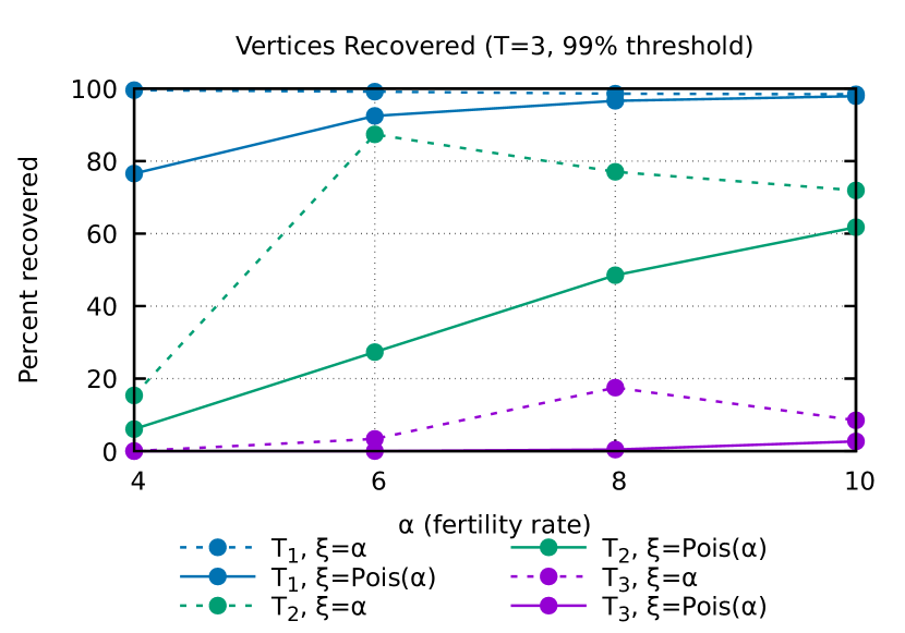
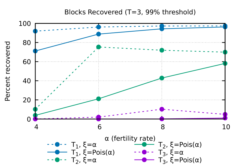
Figure 1: Average percent vertices and blocks 0.99-successfully reconstructed in each generation

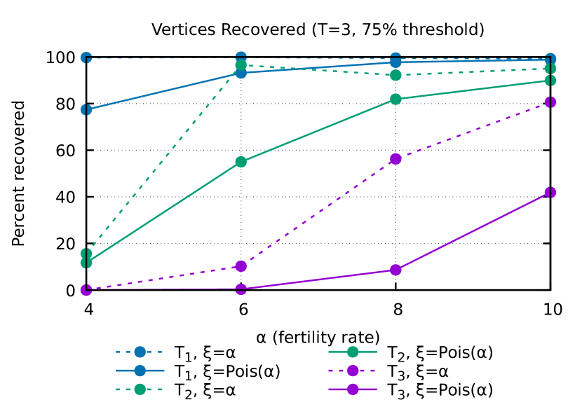
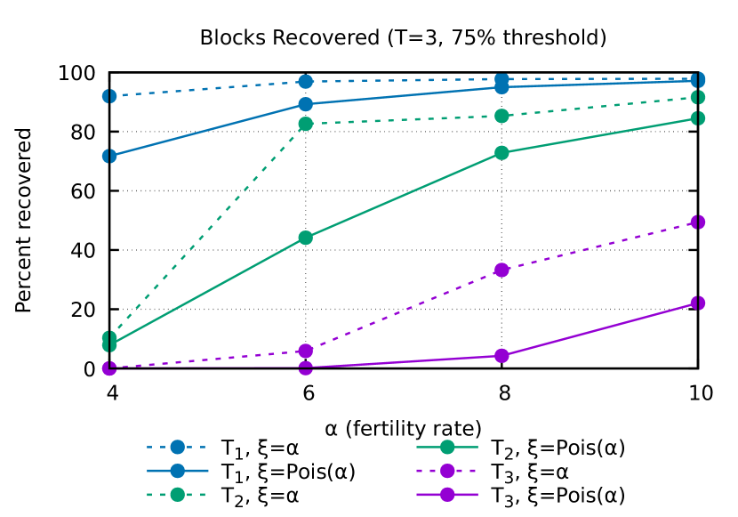
Figure 2: Average percent vertices and blocks 0.75-successfully reconstructed in each generation

5.2 Decline at $\boldsymbol{T=4}$

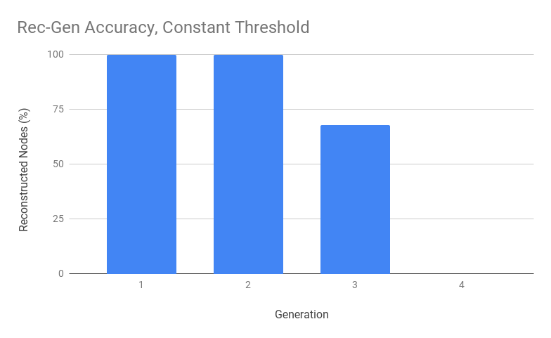
(a) Constant threshold

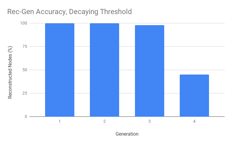
(b) Adjusted threshold

Figure 3: Vertices 0.5-reconstructed by Rec-Gen for a $T=4$ pedigree, with both the default $21\%$ siblinghood threshold (a) and a manually optimized siblinghood threshold (b). Note that 0 nodes are reconstructed in generation 4 in (a).

As demonstrated in Figure 3 (a), Rec-Gen appears to encounter major difficulties by the fourth generation, failing to recover even a single founding node in our simulations. This failure seems to be precipitated by a rapid decline in accuracy of reconstructed blocks, as shown in Figure 4. Recall that symbol collection requires that triples share at least $21\%$ of their blocks to be identified as siblings. In generations 0 and 1, the distribution of shared reconstructed blocks for sibling triples lies entirely above the $21\%$ threshold. By generation 2, it shifts slightly to the left so that some siblings are not recognized (and, as a result, not all of the generation 3 is reconstructed). In generation 3, there are two clusters in the distribution of shared triples: one at 0% and one around 10%. The cluster at 0% is the result of the members of generation 3 who were not reconstructed at all; the rest of the distribution consists of the remaining triples, which still share distinctly more blocks than non-sibling triples, but fewer than 21%.

When we manually set the siblinghood threshold to decay with each generation to match the accumulation of errors, we can extend the number of generations for which Rec-Gen accurately reconstructs the topology. Figure 3 (b) demonstrates the improvements when using the siblinghood thresholds 21%, 21%, 17%, 4% for generations 0, 1, 2, and 3 respectively.

This experiment implies that the step that introduces the most error into Rec-Gen is the symbol-collection step. In reality, we cannot easily manually adjust the siblinghood threshold, because the optimal threshold varies from pedigree to pedigree and may be difficult to determine without knowledge of the true pedigree topology. We can further assume that these errors are largely the result of failure of the combinatorial Rec-Gen algorithm to correctly handle inbreeding. We confirm this assumption by running Rec-Gen on a large pedigree constructed as though it were a section sampled from an infinitely wide pedigree — indeed, Rec-Gen has almost perfect accuracy in this case, as expected (the only errors were the result of blocks that were not passed down to any descendants, which can happen with frequency $1/2^{\alpha}$). We therefore wish to improve the robustness of the symbol-collection step against inbreeding.

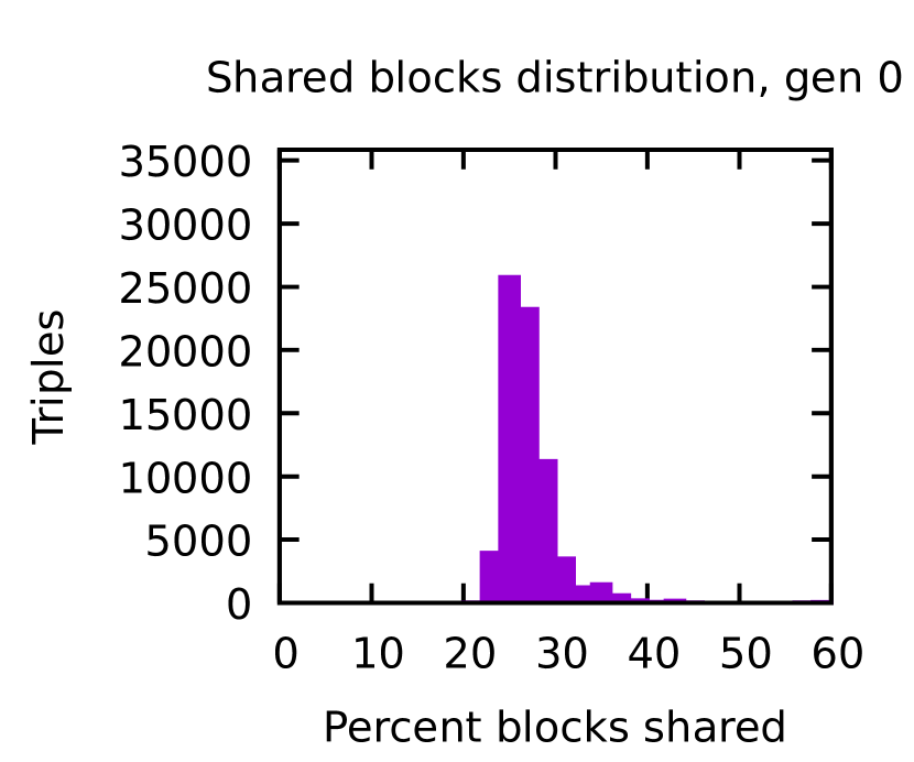
(a) Extant

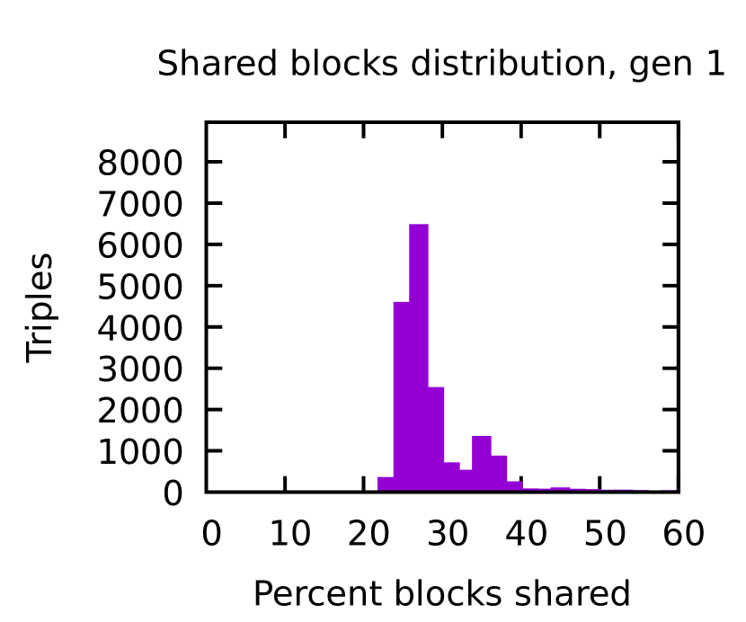
(b) Parents

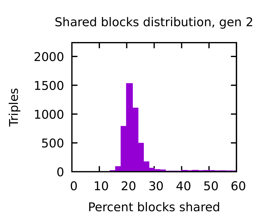
(c) Grandparents

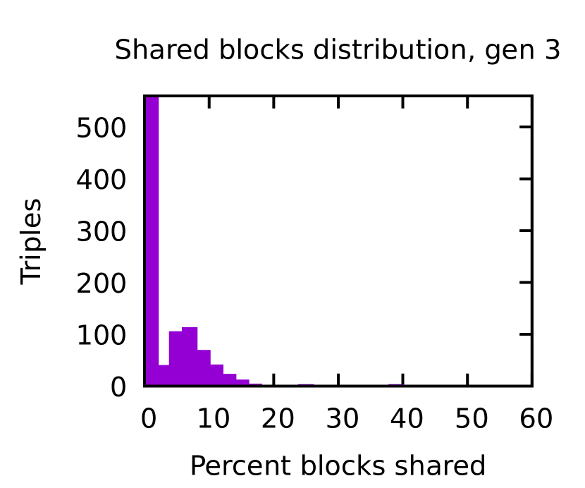
(d) Founder’s children

Figure 4: Distribution of percent reconstructed blocks shared in all triples for a $T=4$ pedigree.

6 Belief Propagation

To improve the empirical accuracy of the symbol collection step, we replace the original combinatorial symbol collection algorithm with a single pass of a Belief-Propagation (BP) algorithm for recovering the genetic information of pedigrees. BP is a message-passing algorithm for inference that is most successful in locally tree-like models. Mezard and Montanari [12] give the BP equations in the following setting:

• $\mathbf{x}$ is a tuple of $N$ variables $\left(x_{1},\dots,x_{N}\right)$ assuming values from the finite alphabet $\mathcal{X}$.

• There are $M$ constraints in the form of the marginals $\psi_{1},\dots,\psi_{M}$ governing the distribution of values assumed by $\mathbf{x}$, so that the probability distribution of $x$ satisfies

  $$p(\mathbf{x})\cong\prod_{a=1}^{M}\psi_{a}\left(\mathbf{x}_{\partial a}\right)$$

  where $\mathbf{x}_{\partial a}=\left\{x_{i}:i\in\partial a\right\}$ and $\partial a\subseteq[N]$ is the set of variable indices constrained by $\psi_{a}$ (here, the notation $x\cong y$ denotes that the two functions $x,y:\mathcal{X}\to\mathbb{R}$ are equal down to a constant factor).

In this context, the relationships between variables can be modelled by a bipartite graph in which each vertex representing a variable $x_{i}$ has an edge to each ‘factor vertex’ representing a constraint $\psi_{a}:i\in\partial a$; this graph is called the factor graph. The BP equations that permit approximation of the marginal distribution of each variable govern ‘messages’ sent over the edges of the factor graph at each time step $t+1$:

• Message from the $j$th variable to the $a$th factor:

  $$\nu_{j\to a}^{(t+1)}\left(x_{j}\right)\cong\prod_{b\in\delta j\setminus a}\widehat{\nu}_{b\to j}^{(t)}\left(x_{j}\right)$$

• Message from the $a$th constraint to the $j$th variable:

  $$\widehat{\nu}_{a\to j}^{(t)}(x_{j})\cong\sum_{\mathbf{x}_{\partial a\setminus j}}\psi_{a}\left(\mathbf{x}_{\partial a}\right)\prod_{k\in\partial a\setminus j}\nu_{k\to a}^{(t)}\left(x_{k}\right)$$

The estimate for the marginal distribution of variable $i$ at time $t$ is

$$\nu_{i}^{(t)}\left(x_{i}\right)\cong\prod_{a\in\partial i}\widehat{\nu}_{a\to i}^{(t-1)}\left(x_{i}\right)$$

If the factor graph is a tree, then BP is known to be exact — that is, the values $\nu_{i}$ converge, and they converge precisely to the true marginals of the variables. Moreover, the exact marginals can be computed with BP in linear time in the tree case, as $\nu_{i}$ assume the values of the marginals of $x_{i}$ after two passes through the tree, as described in Ref. 12.

For our modified symbol-collection step, we effectively complete one BP sweep (half of the tree algorithm) independently for each position in the genome. Let $G$ be the set of all genes, $\mathbf{ch}\left(v\right)$ be the tuple of children of vertex $v$, $0<\varepsilon<1$ be some constant that represents the probability of an error in the topology of the reconstruction, $\mathbf{g}_{v}$ be the variable the value of which is the pair of genes in a given block of vertex $v$, and $\nu_{v}$ be a function from unordered pairs from $G$ to the unit interval, the BP estimate of the marginal distribution of $\mathbf{g}_{v}$.

For each extant vertex $v$ with gene $g$, we introduce a constraint

$$\psi\cong\mathbb{I}_{\mathbf{g}_{v}=(g,g)}$$

For each nonextant vertex $v$, we introduce a constraint indicating that a child of $v$ is an anomaly in the topology (shares no genes with $v$) with probability $\varepsilon$:

$$\psi\cong\varepsilon^{\scalebox{0.75}{$|\{u\in\mathbf{ch}\left(v\right):\mathbf{g}_{v}\cap\mathbf{g}_{u}=\varnothing\}|$}}$$

Then the computed values of $\nu_{v}$ are as follows. For extant couples $v$ with gene $g$, we have

$$\nu_{v}(g_{1},g_{2})\cong\mathbb{I}_{g_{1}=g_{2}=g}$$

And for nonextant couples $v$

$$\nu_{v}(g_{1},g_{2})\cong\sum_{\mathbf{g}\in(G^{2})^{|\mathbf{ch}\left(v\right)|}}\varepsilon^{\scalebox{0.75}{$|\{i\in[1,|\mathbf{ch}\left(v\right)|]:\{g_{1},g_{2}\}\cap\mathbf{g}_{i}=\varnothing\}|$}}\prod_{i\in[1,|\mathbf{ch}\left(v\right)|]}\nu_{\mathbf{ch}\left(v\right)_{i}}(\mathbf{g}_{u})$$

We record the gene pair with the highest probability according to $\nu_{v}$ as the genes reconstructed for couple $v$.

Computing $\nu_{v}$ directly would be computationally inefficient — worse than $O\left(|G|^{2\alpha}\right)$ on expectation, as $|\mathbf{ch}\left(v\right)|$ is Poisson-distributed with parameter $\alpha$. We can substantially improve this runtime by computing the probability distribution by summing over the number of children indicating topology errors, rather than over all possible assignments of genes. To do this, we construct a DP table $\mathbf{DP}(g_{1},g_{2})_{i,j}$ that stores, for the first $i$ children, the probability that $j$ of them indicate topology errors. The recursive definition follows:

$$\mathbf{DP}(g_{1},g_{2})_{i,j}=\left\{\;\begin{aligned} &\mathbb{I}_{j=0}&i=0\\ &\mathbf{DP}(g_{1},g_{2})_{i-1,j-1}\sum_{(h_{1},h_{2})\in G^{2}}\mathbb{I}_{\{h_{1},h_{2}\}\cap\{g_{1},g_{2}\}=\emptyset}\nu_{\mathbf{ch}\left(v\right)_{i}}(h_{1},h_{2})\;+&\\ &+\mathbf{DP}(g_{1},g_{2})_{i-1,j}\sum_{(h_{1},h_{2})\in G^{2}}\mathbb{I}_{\{h_{1},h_{2}\}\cap\{g_{1},g_{2}\}\neq\emptyset}\nu_{\mathbf{ch}\left(v\right)_{i}}(h_{1},h_{2})&i>0\end{aligned}\right.$$

Once we have computed the values of this table for $i=|\mathbf{ch}\left(v\right)|$, we can compute $\nu_{v}$:

$$\nu_{v}(g_{1},g_{2})\cong\sum_{j=0}^{|\mathbf{ch}\left(v\right)|}\varepsilon^{j}\cdot\mathbf{DP}(g_{1},g_{2})_{|\mathbf{ch}\left(v\right)|,j}$$

Constructing the DP table takes $O\left(\alpha|G|^{4}\right)$ time per block, which dominates the runtime of computing the marginals by this method. We can further reduce the runtime by directly maintaining the marginal probability that some single gene appears in each node (in addition to the probability estimate over pairs of genes $\nu_{v}$):

$$S_{v}(g)=\sum_{g^{\prime}\in G}\nu_{v}(g,g^{\prime})$$

Then we can compute the DP as below:

$$\mathbf{DP}(g_{1},g_{2})_{i,j}=\left\{\;\begin{aligned} &\mathbb{I}_{j=0}&i=0\\ &\mathbf{DP}(g_{1},g_{2})_{i-1,j}\left(S_{v}(g_{1})+\mathbb{I}_{g_{1}\neq g_{2}}(S_{v}(g_{2})-\nu_{\mathbf{ch}\left(v\right)_{i}}(g_{1},g_{2}))\right)\;+\\ &+\mathbf{DP}(g_{1},g_{2})_{i-1,j-1}\left(1-(S_{v}(g_{1})+\mathbb{I}_{g_{1}\neq g_{2}}(S_{v}(g_{2})-\nu_{\mathbf{ch}\left(v\right)_{i}}(g_{1},g_{2})))\right)&i>0\end{aligned}\right.$$

Computing the DP table in this manner requires only $O\left(\alpha|G|^{2}\right)$ time.

However, as presented, the BP sweep for symbol collection has a memory complexity of $O\left(|G|^{2}\right)$ per block per node, which in practice is prohibitive even for pedigrees with relatively small founding populations. To reduce the memory complexity by a factor of $|G|$, we make the simplifying assumption that the probability that some vertex $v$ has at least one of a pair of genes $g_{1},g_{2}$ approximately equals $S_{v}\left(g_{1}\right)+S_{v}\left(g_{2}\right)$; this permits us to store only the marginal probabilities over single genes, rather than the entire distribution over pairs of genes.

The DP values are then calculated as follows:

$$\mathbf{DP}(g_{1},g_{2})_{i,j}=\left\{\;\begin{aligned} &\mathbb{I}_{j=0}&i=0\\ &\mathbf{DP}(g_{1},g_{2})_{i-1,j}\left(S_{v}(g_{1})+\mathbb{I}_{g_{1}\neq g_{2}}S_{v}(g_{2})\right)\;+\\ &+\mathbf{DP}(g_{1},g_{2})_{i-1,j-1}\left(1-(S_{v}(g_{1})+\mathbb{I}_{g_{1}\neq g_{2}}S_{v}(g_{2})\right)&i>0\end{aligned}\right.$$

On small pedigrees, this assumption does not produce a decrease in reconstruction accuracy. We also show that simulations on large pedigrees, which are impractical with the $O\left(|G|^{2}\right)$ per-block memory complexity, perform well.

We also implement a relatively simple parsimony-based symbol collection step, which greedily takes the genes that entail the fewest topology errors.

7 Simulation Results for BP

Experiments using simulated data generated as described in Section 4.1 indicate that using BP or Parsimony instead of the combinatorial symbol-collection step of Rec-Gen significantly improves accuracy and permits substantial recovery of the founding populations of $T=4$ pedigrees without manual intervention in the siblinghood threshold. Figures 5 and 6 show the reconstruction accuracy of BP with two values of $\epsilon$ (0.01 and 0.001), parsimony, and the original Rec-Gen symbol-collection step. Parsimony and both instances of BP have similar accuracy, which past the grandparent generation is significantly better than that of the original Rec-Gen. BP with $\epsilon=0.01$ tends to slightly outperform BP with $\epsilon=0.001$ and parsimony. These results indicate that BP is more robust against inbreeding than the combinatorial Rec-Gen. While parsimony is a simple approximation of BP, its reliability decreases when the distribution of fertilities is non-constant.

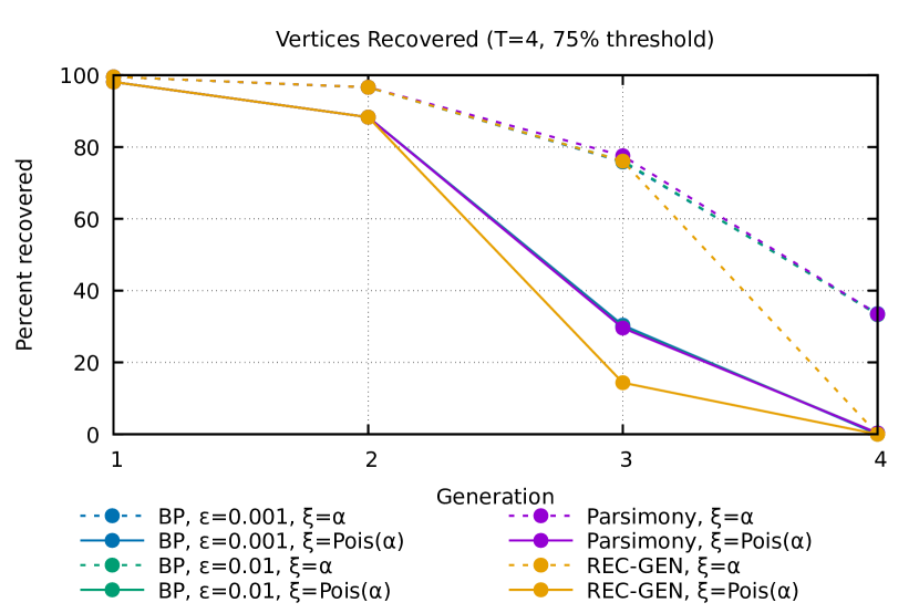
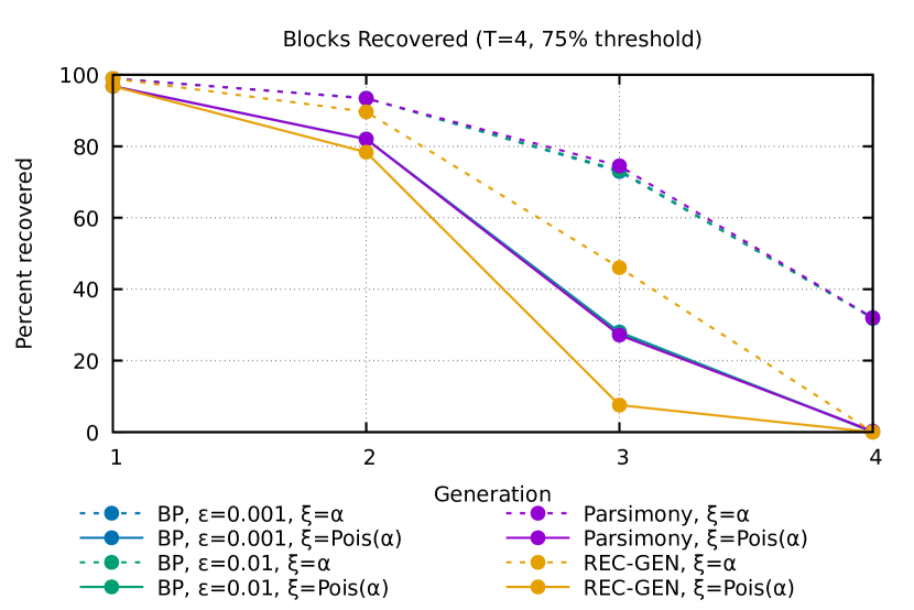
Figure 5: Average percent vertices and blocks 0.75-successfully reconstructed using each of four different procedures for symbol collection in each generation of $T=4$ pedigrees

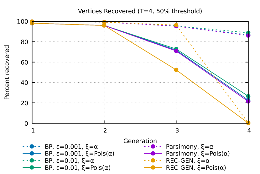
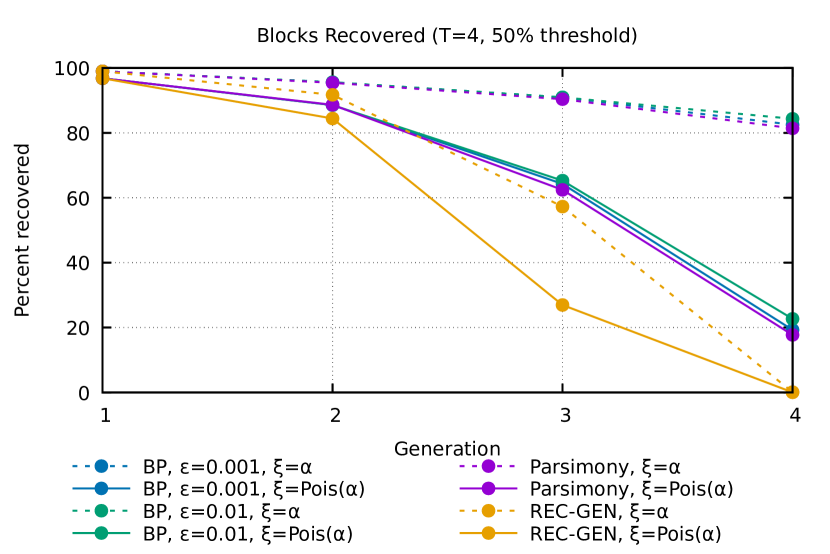
Figure 6: Average percent vertices and blocks 0.50-successfully reconstructed using each of four different procedures for symbol collection in each generation of $T=4$ pedigrees

8 Discussion

The changes to the Rec-Gen algorithm of Ref. 1 presented in this paper contribute significant improvements in practical efficiency and accuracy on simulated pedigree data without sacrificing many of the original algorithm’s theoretical guarantees. We show how to reduce the complexity of the sibling-identification step from cubic in the size of the extant population to essentially quadratic while continuing to use triples as the basis for reconstructing sibling relations and replace the combinatorial genome reconstruction step with a significantly faster and more accurate Belief Propagation procedure; this Belief Propagation procedure is also more accurate than parsimony when the distribution of fertilities is not constant.

Adaptation of our ideas to real-world data is beyond the scope of this work as our model assumes well-defined generations, high fertilities, and no phasing. However, we believe that the presented contributions can be used in practical tools for reconstruction.

Source code and simulation data are available at https://github.com/dvulakh/RecGen

References

- [1] Y. Kim, E. Mossel, G. Ramnarayan and P. Turner, Efficient reconstruction of stochastic pedigrees (2020).
- [2] M. Steel and J. Hein, Reconstructing pedigrees: a combinatorial perspective, Journal of theoretical biology 240, 360 (2006).
- [3] B. D. Thatte and M. Steel, Reconstructing pedigrees: a stochastic perspective, Journal of theoretical biology 251, 440 (2008).
- [4] E. A. Thompson, Statistical inference from genetic data on pedigrees, NSF-CBMS Regional Conference Series in Probability and Statistics 6, i (2000).
- [5] B. Kirkpatrick, S. C. Li, R. M. Karp and E. Halperin, Pedigree reconstruction using identity by descent, Journal of Computational Biology 18, 1481 (2011).
- [6] D. He, Z. Wang, B. Han, L. Parida and E. Eskin, Iped: inheritance path-based pedigree reconstruction algorithm using genotype data, Journal of Computational Biology 20, 780 (2013).
- [7] E. A. Thompson, Identity by descent: variation in meiosis, across genomes, and in populations, Genetics 194, 301 (2013).
- [8] D. He, Z. Wang, L. Parida and E. Eskin, Iped2: Inheritance path based pedigree reconstruction algorithm for complicated pedigrees, in Proceedings of the 5th ACM Conference on Bioinformatics, Computational Biology, and Health Informatics, BCB ’14 (Association for Computing Machinery, New York, NY, USA, 2014).
- [9] D. Shem-Tov and E. Halperin, Historical pedigree reconstruction from extant populations using partitioning of relatives (prepare), PLoS computational biology 10 (2014).
- [10] J. Huisman, Pedigree reconstruction from snp data: parentage assignment, sibship clustering and beyond, Molecular ecology resources 17, 1009 (2017).
- [11] J. Wang, Pedigree reconstruction from poor quality genotype data, Heredity 122, 719 (2019).
- [12] M. Mezard and A. Montanari, Information, Physics, and Computation (Oxford University Press, Inc., USA, 2009).