Noise-induce coexisting firing patterns in hybrid-synaptic interacting networks

Abstract

Synaptic noise plays a major role in setting up coexistence of various firing patterns, but the precise mechanisms whereby these synaptic noise contributes to coexisting firing activities are subtle and remain elusive. To investigate these mechanisms, neurons with hybrid synaptic interaction in a balanced neuronal networks have been recently put forward. Here we show that both synaptic noise intensity and excitatory weights can make a greater contribution than variance of synaptic noise to the coexistence of firing states with slight modification parameters. The resulting statistical analysis of both voltage trajectories and their spike trains reveals two forms of coexisting firing patterns: time-varying and parameter-varying multistability. The emergence of time-varying multistability as a format of metstable state has been observed under suitable parameters settings of noise intensity and excitatory synaptic weight. While the parameter-varying multistability is accompanied by coexistence of synchrony state and metastable (or asynchronous firing state) with slightly varying noise intensity and excitatory weights. Our results offer a series of precise statistical explanation of the intricate effect of synaptic noise in neural multistability. This reconciles previous theoretical and numerical works, and confirms the suitability of various statistical methods to investigate multistability in a hybrid synaptic interacting neuronal networks.

I INTRODUCTION

Multistability or coexistence of several possible final stable states (different attractors) in the nervous system has attracted a increased interest, stemming both from new experimental methods for identifying it and from a growing body of modeling work demonstrating its functional consequence[1]. Many of these studies over several decades have outlined the sources and impact of biological multistability to a better understanding emergence or any dysfunction of brain behavior[2], in particular, associative memory storage, pattern recognition and the pathophysiology of human diseases[3] in both living and artificial neural systems. Multistability have long been of interest, but there still much to be known about their underlying mechanisms in neural systems.

Multistability can arise from two possible sources[4, 5]. The first source is from the deterministic chaos of the neural system. For example, it is generally accepted that inherent instability nature of chaos in neural systems, facilitates the extremely sensitivity to initial condition, to create a rich varity of coexistence of firing patterns. Deterministic chaos also can induce a definite switching between different coexisting states, both at the level of individual neurons and neural networks.The alternative source of multistability is noise. Some studies demonstrate that noise not only induce multistability, but also drive transitions between two or more multistable attractors, in systems of coupled oscillators [6] and in a field-dependent relaxation model[7].Whereas previous studies have focused on neuronal multistability caused by deterministic chaos or stochastic noise in networks of neurons solely connected by chemical or electrical synapses, we focus here on work mainly relating to noise-driven coexisting firing patterns in a hybrid synaptic interacting balanced neural networks.

Biologically relevant sources of noise permeating every level of the nervous system from the perception of sensory signals to the generation of motor responses, have beed evidenced by experimental data (see review[8, 9]). For external sensory stimuli to brain, all forms of perception such as chemical sensing and vision are affected by thermodynamic noise, which is namely sensory noise. Sources of sensory noise include intrinsically noisy from external sensory stimuli and transducer noise that is generated during the amplification process[9, 10]. It is well known that neuronal activity is intrinsically irregular in the generation of action potentials, their axonal propagation, network interactions, and the synaptic transmission that follows. This is due to the stochastic opening and closing of ion channels,the constant bombardment of synaptic inputs and synaptic unreliability[11]. This type of neuronal noise is cellular noise, which can be of channel noise, synaptic noise and network interactions[8, 9]. Multiple factors contribute to cellular noise, including changes in the interal states of neurons and networks or random processes inside neurons and neuronal networks. At end, experimental evidence also suggests the nervous system has to act in the presence of noise in sensing, information processing and movement in the behavioural task, such as catching a ball. This type sources of neural variability in the force generated by motor neurons and muscle fibres is motor noise[12]. While observation of neural noise has been explored in multiple experimental studies, it is not yet well understood the diverse roles of noise in neural computation and brain function based on neuronal theories and models.

Noise commonly assumed to be a nuisance, and nervous systems develop strategies to filter it. Besides, noise can also induce new organized behaviors in systems that lack in deterministic conditions(see reviews [8, 9, 11]). Several strategies have been adopted to use noise in this fashion. Most notably,in spike-generating type neurons, noise can transform threshold nonlinearities by making subthreshold inputs more likely to cross the threshold, and thus this is more easy to generate a spike. This facilitates spike initiation and can improve neural-network behaviour[13]. In addtion, studies of both experiments and theoretical models revealed that a subthreshold sensory signal has a better chance of being detected when noise is added, broadly known as stochastic resonance[14, 9]. For a small amount of noise, the sensory signal does not cause the system to cross the threshold and few signals are detected. At large noise levels, the response is dominated by the noise. For intermediate noise intensities, however, the noise allows the signal to reach the threshold for detection but does not swamp it. Therefore, stochastic resonance has been evidenced to enhance processing both in theoretical models of neural systems and in experimental neuroscience. Moreover, neuronal networks that have formed in the presence of noise will be more robust and explore more states, which will facilitate learning and adaptation to the changing demands of a dynamic environment. In all, the present of noise leading to spontaneous order in neural systems include stochastic resonance, noise-induced phase transitions, and noise-induced bistability. Nevertheless, the contribution of noise to coexisting firing patterns and stochastic switching between these attractor basins in the banance neural systems have not been systematically explored yet.

Computational models studies show that itinerant dynamics can be basically to uncover mechanisms of coexisting attractor basins and stochastic switching between multistable states. Several dynamical approaches support itinerant dynamics including chaotic itinerancy, heteroclinic cycling, and multistable switching[1, 4, 15]. Chaotic itinerancy and heteroclinic cycling focus on deterministic dynamics, in which either a chaotic attractor or a series of saddle points connected by heteroclinic orbits allow the system not to settle in a attractor (or saddle) but instead visit one after the other. Thus, chaotic deterministic trajectories is first possible sources of itinerant dynamics. It is well known that chaos can emerge in insolate neurons or complex neural systems in different scales of networks size[16, 17, 18]. On the other hand, multistable switching implies the coexistence of multiple stable attractors.Thus, neural noise is second possible sources of itinerant dynamics,causing switching between different attractors.

All of these previous studies only identify the essential mechanisms for noise,chaos or comparation of them driven multistability of networks sole connected by electrical or chemical synapses. In this work, our main motivation is to identify the mechanisms of noise-induced coexisting firing patterns in a hybrid synaptic interacting balanced neuronal networks – combination connection and effection of electrical and chemical synapses. The excitatory population of balanced network is communicated through chemical synapses in a way of small-world topology, and adjacent excitatory cells of small-world neural network is also connected by electrical synapses. The nodes in our network are the Wang-Buzsaki model as a general model of mammalian neuronal excitability[19]. In case of fixed synaptic noise intensity, our previous research showed that the existence of electrical synaptic connections to excitatory population can cause various firing patterns of interest by slightly changing the chemical synaptic weights[20].However,the effection of noise together with other facts with complexity, such as synaptic weights,types of synapses and so on, to neural firing pattern in this balanced network have not been well investigated.

In this paper, we study the emergence of coexisting firing patterns in an excitatory-inhibitory (E/I) balanced network, combining the effect of synaptic noise and chemical connections. We report that there are two typical forms of coexisting firing patterns obeserved in this balanced networks, that are time-varying coexistence and parameter-varying coexistence. The time-varying coexisting firing patterns is typically metstable state, normally coexistence of synchronous state and traveling wave or alternation between those two states. The parameter-varying coexistence in this balanced neural networks is accompanied by coexistence of coherence and incoherence firing state with slightly varying control parameters. With further investigation, we find that the emergence of time-varying coexistence has been observed under suitable parameters settings of noise intensity and excitatory synaptic weight, while latter case, the coexisting neuronal behaviour is a result of systems parameters varying, since neural network can display a single collective behaviour or metstable firing state for fixed values of systems parameters. Our findings imply that synaptic noise intensity and excitatory weights can make a greater contribution than other factors, such as variance of synaptic noise, to the coexistence of various firing states with slight modification parameters.

II Models and methods

Wang-Buzsáki model. The Wang-Buzsaki (WB) model[19, 21]resembles the dynamics of fast-spiking neurons in the cortex and hippocampus, and it is used here only as a general model of mammalian neuronal excitability. The Wang-Buzsáki model has three states variables for each nodes: membrane potential $V$, the variable $h$, $n$ corresponding to the spikes-generating $Na^{+}$ and $K^{+}$ voltage-dependent ion currents. The variable $m$ is considered to be instantaneous. The neuronal dynamics of each node can be described as :

$$C_{m}\frac{dV}{dt} =-I_{Na}-I_{K}-I_{L}-I_{Syn}+I_{app}$$

$$\frac{dh}{dt} =\phi(\alpha_{h}(1-h)-\beta_{h}h)$$

$$\frac{dn}{dt} =\phi(\alpha_{n}(1-n)-\beta_{n}n)$$ (1)

Where $I_{L}=g_{L}(V-E_{L})$, $I_{Na}=g_{Na}m^{3}_{\infty}h(V-E_{Na})$ and $I_{K}=g_{K}n^{4}(V-E_{K})$ represent the leak currents, transient sodium currents, and the delayed rectifier currents. $I_{syn}$ stands for the synaptic currents and $I_{app}$ (=0 in our simulations) is the injected currents (in $\mu A/cm^{2}$). The parameters $g_{L}$, $g_{Na}$, $g_{K}$ are the maximal conductance density, $E_{L}$, $E_{Na}$, $E_{K}$ are the reversal potential and function $m_{\infty}$ is the steady-state activation variables $m$ of the Hodgkin-Huxley type[22]. The default value of these parameters and functions are shown in Table 1.

To better understand and exhibit effects of various types of noise on WB neuron, three examples of voltage time courses of both deterministic and stochastic WB neurons have well been replotted in Fig.1B. Deterministic WB model, Eq.(II), has been successfully applied to describe the dynamics of periodic regular firing for mammalian neuronal excitability in Fig.1B,Top. With further consideration of input noise to WB neuron, such as sensory noise or external input noise, isolated WB neuron can generate higher frequecy but irregular spikes (in Fig.1B,mid) when $I_{app}=\mu+\sigma\eta(t)$, where $\mu$ and $\sigma$ are, respectively, the mean and SD of the process and $\eta(t)$ is a Gaussian white-noise variable. More importantly, many previous studies showed that neuronal activity is intrinsically irregular in the generation of action potentials due to channel noise, synaptic noise and network interactions[11, 8, 9]. For ease of comparison with the previous irregular firing, example of intrinsically irregular firing induced by channel noise $g_{Kstoch}=g_{K}*No/Nk$ (note that $Nk=3$ and $No$ are the number of K+ channels and open channels at equilibrium state), has been shown clearly in Fig.1B,bottom. As shown in Fig.1B, the former irregular firing impacted by input noise of continuous-time stochastic processes as Langevin equation, however, the later intrinsically stochastic firing affeced by channel noise in a discrete time set-up of specific open channels. The theoretical underlying mechanisms of generating these significant stochastic neural firing, such as dynamical bifucation, have been so deeply investgated[23, 24]. This study is to find and ascertain the effects of intrinsically stochastic of interest on collective behaviour (e.g coexisting firing patterns) of balance neural networks.

Synaptic dynamics. The neurons in the networks are connected both by electrical and chemical synapses. $I_{SynE,i}$ , $I_{SynI,i}$ stand for total synaptic input currents into neuron $i$ for excitatory population and inhibitory population, respectively, given by:

$$I_{SynE,i}=J_{gap}\vec{C}_{gap}^{i}\cdot\vec{D}^{i}+J_{EE}\vec{L}_{EE}^{i}\cdot\vec{g}_{syn}(V_{i}-E_{synE})+J_{EI}\vec{L}_{EI}^{i}\cdot\vec{g}_{syn}(V_{i}-E_{synI})+\sum_{j=1}^{N_{E}}g_{syn,j}(V_{i}-E_{synE})$$ (2)

$$I_{SynI,i}=J_{II}\vec{L}_{II}^{i}\cdot\vec{g}_{syn}(V_{i}-E_{synI})+J_{IE}\vec{L}_{IE}^{i}\cdot\vec{g}_{syn}(V_{i}-E_{synE})$$ (3)

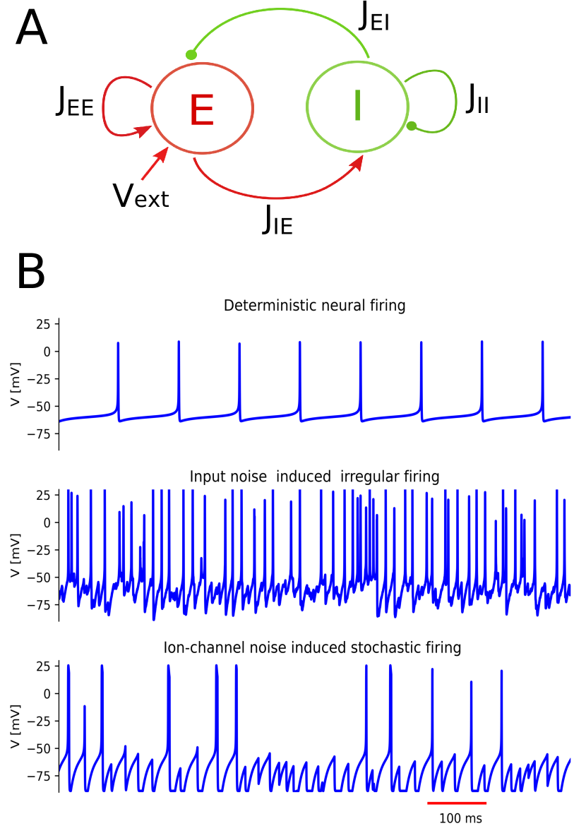
Figure 1: Wang-Buzsáki balance neural network and voltage time course of isolated deterministic and stochastic WB neuron. A. The balanced neural networks containing excitatory (E) and inhibitory (I) population . The synaptic communications between these two populations in the way of all-to-all interconnects. $J_{IE}$ and $J_{EI}$ denote corresponding weights of excitatory and inhibitory synaptic inputs crossing different populations. $J_{EE}$ and $J_{II}$ present the weights of self-excitatory (in a small world topology) and self-inhibitory connections (in a way of all-to-all topology). $\nu_{ext}$ is the external excitatory drive to each neuron in the excitatory population. $J_{gap}$ is weight of electrical synaptic coupling among adjacent neurons in the E-population (not shown here detailly, see Fig.1 in Ref[20]). We fix $J_{II}=0.04$, $J_{IE}=0.01$. B. Top: Action potential of isolated deterministic WB neuron when $I_{app}=0.2$; Middle: irregular neural firing of a WB neuron induced by Gaussian white-noise when $I_{app}=\mu+\sigma\eta(t)$, where $\mu$ and $\sigma$ are, respectively, the mean and SD of the process and $\eta(t)$ is a Gaussian white-noise variable; Bottom: stochastic neural firing caused by ion channel noise, given by $g_{Kstoch}=g_{K}*No/Nk$ (note that $Nk=3$ and $No$ are the number of K+ channels and open channels at equilibrium state).

The dot products in Eq.(2) are electrical synaptic inputs, self-excitatory synaptic inputs, inhibitory synaptic inputs, and last term of Eq.(2) is external excitatory synaptic inputs. The dot products in Eq.(3) represent self-inhibitory synaptic inputs and excitatory synaptic inputs.The vector $\vec{C}_{gap}^{i}=({c}_{gap}^{i1},{c}_{gap}^{i2},\cdots,{c}_{gap}^{ij})$ and $\vec{D}^{i}=(V_{i}-V_{1},V_{i}-V_{2},\cdots,V_{i}-V_{j})$ stand for connection vectors and their diffusive coupling induced by electrical synapses. The elements in vector $\vec{g}_{syn}=(g_{syn,1},g_{syn,2},\cdots,g_{syn,j})$ are chemical synaptic conductances. The elements of vector $\vec{L}_{mn}^{i}=(l_{mn}^{i1},l_{mn}^{i2},\cdots,l_{mn}^{ij})$ denote the connections between the $i$th neurons of the $m=E,I$ (excitatory, $E$ or inhibtory $I$) population and the $jth$ neurons of the $n=E,I$ population. More detailed explanations are that: $l_{EE}^{ij}$ and $l_{II}^{ij}$ are elements of self-excitatory and self-inhibitory connections, whereas $l_{IE}^{ij}$ (or $l_{EI}^{ij}$) is element of the all-to-all matrices of excitatory-to-inhibitory connections (or vice versa). $C_{gap}^{ij}$ is element of electrical synaptic connections in excitatory population. The parameters $J_{EE},J_{II},J_{IE},J_{EI},J_{gap}$ indicate the corresponding synaptic weights of connections $l_{EE}^{ij},l_{II}^{ij},l_{IE}^{ij},l_{EI}^{ij},C_{gap}^{ij}$. Here $L_{mn}^{ij}=1$ (or $0$) is (or not) connections (also see Ref[20]). The default network parameters used here are shown in Table 2.The updating rule of chemical synaptic conductances,$g_{syn}$, has been described in Appendix A.2.

Network connectivity. We consider a balanced neural network, consisting of $N_{E}=1000$ excitatory and $N_{I}=250$ inhibitory neurons for this paper shown in Fig.1. The excitatory population itself is connected by excitatory synapses in small world topology and its adjacent neurons are inter-connected by gap junctions. The inhibitory population itself is only with all-to-all interaction by inhibitory synapses. The small-world topology for excitatory population is implemented as two basic steps of the standard algorithm (See Ref.[25]).

Network Activity Characterization. In this paper we first use the synchronization index, $\chi$, to account for the synchronization level of the neural activity of the considered networks[26, 20], where:

$$\chi^{2}=\dfrac{N\sigma_{V(t)}^{2}}{\sum_{i=1}^{N}\sigma_{V_{i}(t)}^{2}}$$ (4)

Here $V(t)=\frac{1}{N}\sum_{i=1}^{N}V_{i}(t)$ denotes population average of the membrane potential $V_{i}(t)$. $\sigma_{V(t)}$ and $\sigma_{V_{i}(t)}$ are standard deviation of $V(t)$ and the membrane potential traces $V_{i}(t)$ over time. $\chi$ is $1$ when all the neurons have the same trajectory and $0$ for an incoherent state when the fluctuations of $V(t)$ are $0$.

To further investigate the global dynamical behavior of the neural networks, we further introduce the order parameter[27, 28], $R$, together with its the variance in time, metastability[29, 18, 20], $Met$, given by:

$$R =\left\langle\left|\frac{1}{N_{E}}\sum_{k=1}^{N_{E}}e^{2\pi i[(t-t_{k}^{n})/(t_{k}^{n+1}-t_{k}^{n})]}\right|\right\rangle$$ (5)

$$Met =\frac{1}{T}\sum\limits_{t\leq\Delta t}\left(\phi_{c}(t)-R\right)^{2}$$ (6)

The angle brackets in Eq.(5) is the temporal average value of that quantity and $2\pi[(t-t_{k}^{n})/(t_{k}^{n+1}-t_{k}^{n})]$ is the phase of each neurons in the excitatory population. $t_{k}^{n}$ is coming time of the $n$th spikes of neurons $k$ (and thus $t_{k}^{n+1}$ is time of the following $(n+1)$th spikes). The closer to $R=0(1)$ becomes, the more asynchronous (synchronous) the dynamics is. The global metastability[29], $Met$ (Eq.(6)) is used here to quantify metastability and chimera-likeness of the observed dynamics. Metastability is $0$ if the system is either completely synchronized or completely desynchronized – a high value is present only when periods of coherence alternate with periods of incoherence.

We next introduce SPIKE-Synchronization (SPIKE-Syn) for quantifying similarity in terms of the fraction of coincidences between two spike trains[30, 31]. A coincidence indicator $C_{i}^{1,2}$ for SPIKE-Syn is described for every spike of the two spike trains $S_{i}^{1,2}$. The $C_{i}=1$ if the spikes at $t_{i}$ is part of a coincidence and $C_{i}=0$ if not. The value of the coindidence indicator is then given by:

$$C_{i}^{1}=\left\{\begin{aligned} 1&\quad\text{if}\min_{j}(|t_{i}^{1}-t_{j}^{2}|)<\tau_{ij}^{1,2}\\ 0&\quad\text{otherwise}\end{aligned}\right.$$ (7)

Where $\tau_{ij}^{1,2}=\frac{1}{2}\min\{\nu_{i}^{1},\nu_{i-1}^{1},\nu_{j}^{2},\nu_{j-1}^{2}\}$ is an adaptive coincidence window according to the local firing rate. the interspike intervals are given as $\nu_{i}^{1,2}=t_{i+1}^{1,2}-t_{i}^{1,2}$. The coincidence indicator for the second spike train $C_{i}^{2}$ is computed as the same way. The spike-synchronization profile is then given by the discrete function in terms of the pooled coincidence indicators $\{C_{k}\}=\{C_{i}^{1}\}\cup\{C_{i}^{2}\}$ and spike times $\{t_{k}^{{}^{\prime}}\}=\{t_{i}^{1}\}\cup\{t_{i}^{2}\}$. The pairwise time spike synchronization values (spike$\_$sync$\_$matrix) $s_{c}$,quantifies the fraction of all spikes in the two spike trains that are coincident, given by:

$$s_{c}=\frac{1}{M}\sum_{k=1}^{M}C_{k}$$ (8)

where $M=M_{1}+M_{2}$ denoting the total number of spikes in the pooled spike train. $s_{c}=0$ for spike trains without any coincidences and $s_{c}=1$ if and only if the two spike trains consist only of pairs of coincident spikes. The generalizing coincidence indicators is defined as before: $C_{i}^{n,m}$ is 1 if $\min_{j}(|t_{i}^{n}-t_{j}^{m}|)<\tau_{ij}^{n,m}$ and 0 if not, where $\tau_{ij}^{nm}$ is similar as above. A normalized coincidence counter for each spike of every spike train is given as $C_{i}^{n}=\frac{1}{N-1}\sum_{m\neq n}C_{i}^{n,m}$ obtained by averaging over all $N-1$ bivariate coincidence indicators involving the spike train $n$. Therefore , the multivariate SPIKE-synchronization is described by:

$$S_{C}=\frac{1}{M}\sum_{k=1}^{M}C_{k}$$ (9)

where $M=\sum_{n}^{m}M_{n}$ again denotes the overall number of spikes. The interpretation is very intuitive: SPIKE-Synchronization quantifies the overall fraction of coincidences. It is zero if and only if the spike trains do not contain any coincidences, and reaches one if and only if each spike in every spike train has one matching spike in all the other spike trains.

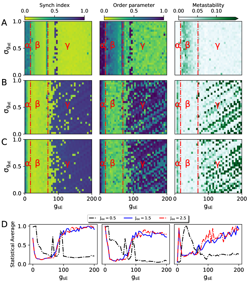
Figure 2: The effect of chemcial synaptic noise among excitatory neurons on coexisting firing patterns in $g_{sE}/\sigma_{g_{sE}}$ parameter space. The variables $g_{sE}$, $\sigma_{g_{sE}}$ are the means and standard deviation of Gaussian distribution uesd here for peak synaptic conductances. In presence of chemical synaptic noise among excitatory neurons can produce significant emergence of neural network state, that are: A.($\alpha$). synchronous firing pattern,($\beta$). metastable state, ($\gamma$).asynchronous firing state; B-C.($\alpha$).coexistence of synchronous and asynchronous firing pattern, ($\beta$).asynchronous firing state, ($\gamma$).coexistence of metastable and synchrony state. D. Statistical average of synchrony index, order parameter and metastability (left to right) over all the $\sigma_{g_{sE}}\in(0,1]$ against $g_{sE}\in(0,200]$. The excitatory synaptic weights of E-population for each row are A. $J_{EE}=0.5$, B. $J_{EE}=1.5$, C. $J_{EE}=2.5$.

III Influence of synaptic noise among excitatory neurons in coexisting firing patterns

Networks with mixed excitatory/inhbitory (E/I) neurons, displaying various firing patterns depending on the presence of gap junction in the E/I balance network, has been well studied in our previous work[20]. In this work, we will investigate the contribution of chemical synaptic noise on coexisting firing patterns of a hybrid synaptic interacting balanced neuronal network. Fig.2A shows collective behaviour of coexisting firing patterns resulting from the simulation of a network consisting on 1,000 excitatory and 250 inhibitory neurons, in a full region of the $g_{sE}/\sigma_{g_{s}E}$ parameter space. We characterized these firing regimes by calculating the synchronization index $\chi$ (in Eq.4) for voltage traces, and the Kuramoto order parameter $R$ for phase synchronization based on spike firing (see Eq.5). We also introduce the metastability $Met$ Eq.(6) to quantify the metastability and coexisting firing pattern of the observed dynamics within the excitatory population. The results from a balanced neuronal network with weaker excitatory connection, when $J_{EE}=0.5$ as a example, is shown in Fig.2A. Fig.2A shows three significant but different phases of collective network states that are synchronization state, time-varying coexisting firing state (or multistable state) and asynchronous state, characterizing behavior of the neuronal networks by means of the synchrony and metastability indexes. The general synchronization index $\chi$ is highly dependent on the means value $g_{sE}$ of Gaussian distribution, displaying three distinct collective behaviour with color regions shown as $\alpha,\beta,\gamma$. However, for a given value of $g_{sE}$, neural firing and synchronization modes of these three regions are robust against different values of noise variance, $\sigma_{g_{sE}}$. This observation suggests that the means $g_{sE}$ of Gaussian distribution as source of synaptic noise make a greater contribution than standard deviation $\sigma_{g_{sE}}$ to neural firing patterns. The synchronization of spikes quantified by order parameter $R$ also shows a similar pattern although these three firing regions appear less homogeneous than in the case of the general index $\chi$. More importantly, the metastability index shows this, with a metastable region separating the synchrony region $\alpha$ and asynchronous region $\gamma$. As predicted by the measurement of statistical methods mentioned above, an increase in mean $g_{sE}$ of peak synaptic conductances causes the appearance of a region $\beta$ with higher metastability as a transition from synchronous to asynchronous firing.

The effect of increasing synaptic weights among excitatory neurons on firing pattern is exhibited in Fig.2B-C).There is a dramatic changes for $\gamma$ regimes in the synchrony measures although this effect is not evenly distributed across the whole parameter space.Region $\gamma$ shows a high increase in synchrony, displaying as speckle pattern of parameter space. As hinted by this speckle pattern, higher values of this pattern, approximately equal to 1, are often characterized by coherent state of activity that can not find the metstable or asynchronous behaviour; whereas the rest region in the speckle pattern is an intermediate synchrony region, indicating metstable state that is characterized by high metastability. In the other words, speckle pattern shown in $\gamma$ indicates the coexistence of synchronous firing and metstable state with slightly varying systems parameters, which is namely parameter-varying coexistence. The more important findings shown in speckle pattern (Fig.2B,C) is that both means $g_{sE}$ and $\sigma_{g_{sE}}$ of Gaussian distribution can play a great role on the neural firing pattern, which is different in case of weaker excitatory weights plotted in Fig.2A. On the contrary, region $\beta$ in Fig.2B,C displays a decrease of synchronization index and order parameter, as a result of increasing the excitatory synaptic weights. The results obtained from metastability (Fig.2B,C) imply that region $\beta$ goes to an asynchronous firing state instead of metstable state in Fig.2A with slight enhencing $J_{EE}$. Region $\alpha$ shows coexistence of synchronous and metastable state (Fig.2B,C) instead of absolutely synchronization, characterized statistical methods mentioned. Finally, in order to further understand the effect of excitatory synaptic weights on neural firing mode, Fig.2D plots statistical average of synchrony index, order parameter and metastability over $\sigma_{g_{sE}}$ with growth of $g_{sE}$. As predicted, the results obtained from $\alpha,\beta,\gamma$ regions are robust with enhancing excitatory connection weights shown in Figs.2B,C. However, when E-population with weak coupling(in Fig.2A), these regions exhibit their opposite impact on neural responses, clarifying that the repetitive firing properties of E-population is greatly affected by excitatory synaptic weights. In all, exploring the $g_{sE}/\sigma_{g_{sE}}$ parameter space under suitable excitatory synaptic weights is beneficial for the emergence of novelty firing patterns, such as parameter-varying coexistence of metastable and synchrony state that can not be observed with weaker excitatory coupling.

In the following, we will examine in more detail the coexistence of several possible firing patterns and their transitions between these firing regimes caused by increasing the means of Gaussian distribution. To do this, we will focus on two values of excitatory strength: $J_{EE}=0.5$ and $J_{EE}=1.5$, roughly sweeping the areas of a widely range $g_{sE}\in(0,200]$.

IV Repetitive firing patterns and transitions between different firing regimes

We then investigated various firing patterns at different excitatory level, to characterize the firing patterns and their transitions between these firing state that represented by $\alpha,\beta,\gamma$ shown in Fig.2. Fig.3 shows the evolution of synchrony of order paramenter for spikes and metastability as $g_{sE}$ is swept from 0 to 200, under weak (Fig.3A,C) and a slightly stronger(Fig.3B,D) excitatory coupling.

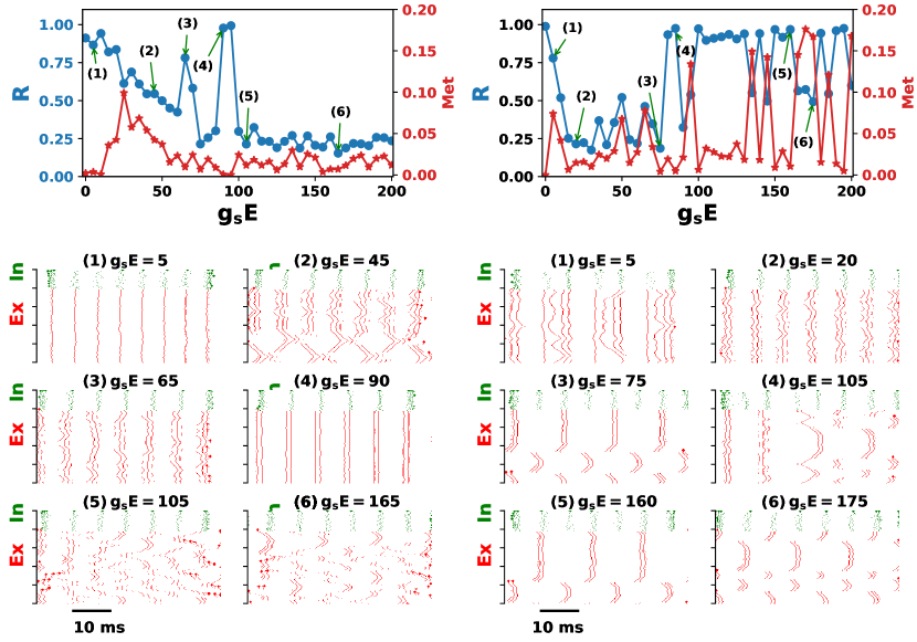
Figure 3: Significant emergence of neural network state and transitions with enhencing synaptic noise under different level of excitatory coupling, where $J_{EE}=0.5$ (A,C) and $J_{EE}=1.5$ (B,D). Red star and blue circle lines represent evolution of order parameters and metastability for excitatory population. C and D show a detail examples of typical spatiotemporal firing patterns that corresponding to letters shown in (A) and (B) in each dynamics regimes as sweeping parameter $g_{sE}$. (a,d): Synchronous states; (c,g,h) Generalized synchrony states; (e,f): asynchronous states; (b,i,j,k,l) Metastable state or chimera-likeness.

With weak (Fig.3A,C) and a little stronger excitatory synaptic coupling (Fig.3B,D), the E-population of balance network usually can go through different phases of network state as variation of $g_{sE}$. The letters a-l in Fig.3C,D represent some examples of various firing pattern for each dynamical regiems that shown in Fig.2. The activities of synchronous, metstable and asynchronous states have been clearly observed looking at variation through $R$ and $Met$. These significant dynamical regimes as well as corresponding transitions can be defined based on the different values of $Met$ . The finer sweep of the means of synaptic noise now allows to observe that the transition between the one-spike synchronous firing pattern (a) and the two-spike synchronous pattern (d) occurs with a little more disordered patterns (b,c). These disordered firing patterns are characterized by high metastability, exhibiting time-varying coexistence of unstable and transient traveling waves. It is worth noting that two-spike synchronous pattern(d) appear here also as a transition to the asychronous firing oscillatory regime(e,f), characterized by low order paramter and metastability when $g_{sE}>95$. In contrast, we repeated the same exploration at a higher level of excitatory strength when $J_{EE}=1.5$ in Fig.3B,D. The resulting varying values of $R$ and $Met$ against $g_{sE}$ , as well as rastor plots, show that the activity of parameter-vaying coexisting firing is incoherent, that are coexistence of generalized synchrony states (g,h) and metstable state (i,j,k,l) at different values of $g_{sE}$. Moreover, we observe that metstable state has been performed as format of coexistence or alternation of interest between synchronous state and traveling wave under suitable parameter values of $g_{sE}$. In all, the main findings in Fig.3 provide supporting evidence that synaptic noise intensity and excitatory level are significant system parameters which play a major role in determining the emergence of the firing patterns, including traveling wave, synchrony state with one-spike (or two-spike), a peculiar coexisting firing patterns (chimera-likeness behavior). More importantly, neural firing transitions between dynamical states also depend on strength of synaptic noise among individual neurons. The more detailed influence of the whole $g_{sE}/J_{EE}$ parameters space on neuronal firing patterns will be systematically studied in section V.

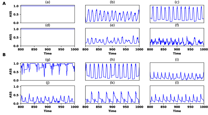
Figure 4: Averaged SPIKE-Sync profile (ASS) for a fixed time window, quantifying similarity and periodicity (or quasi-periodic ) of neuronal firing state in time. Subplots A and B respectively corresponding to the raster plots of spike train that plotted in Fig.3C,D . The letters $a-l$ denote the examples of firing rate in Fig.3 .

So far we have focused on conditions of arising coexisting firing patterns and statistical methods of measuring the degree of synchronization in E-population. We then computed SPIKE-Sync profile in Eq.9 of the excitatory spike strains, as well as average SPIKE-Sync shown as function of time, to quantify similarity and periodicity of neuronal firing state. Fig.4 plots averaged SPIKE-Sync profile (ASS) for a fixed time window to quantify similarity and periodicity of neuronal firing state, that that are shown in Fig.3C,D . With weak coupling (Fig.4A), the balanced neural network exhibited higher correlated spike trains (Fig.4(a),(d)), which is steady-state synchronization characterized by $ASS=1$, in contrast to spike trains in the asynchronous state (Fig.4(e),(f)). As in the asynchronous state, irregular activity with lower value of averaged SPIKE-Sync profile is observed, denoting lower and weaker correlated spike trains along time. More importantly, varying $g_{sE}$ demonstrates that the balanced network also can exhibit similarity, and 1-periodic (or quasi-periodic ) acitivity of great interest (Fig.4(b),(c)), implying again emergence and multistability of time-periodic states in a excitatory population of noise-driving and hybrid synaptic interacting networks (see Fig.3C ).

As predicted in Fig.4B at a higher level of excitatory coupling, the big difference is that only weaker correlated (or uncorrelated) spike trains have been observed from ASS time series with increasing $g_{sE}$. It was surprisely found that the repetitive behaviors with 2-periods are shown in Fig.4(i-l) by the spike train similarity measures of that $ASS<1$, suggesting the emergence of periodic firing patterns accompanying with subthreshold oscillations of some neurons in a excitatory population (compares to i-l in Fig.3D ). Secondly, quasi-periodic firing patterns also has been observed in Fig.4(h). Otherwise, alternative time series of ASS between synchronous and asynchronous state has been shown in Fig.4(g).

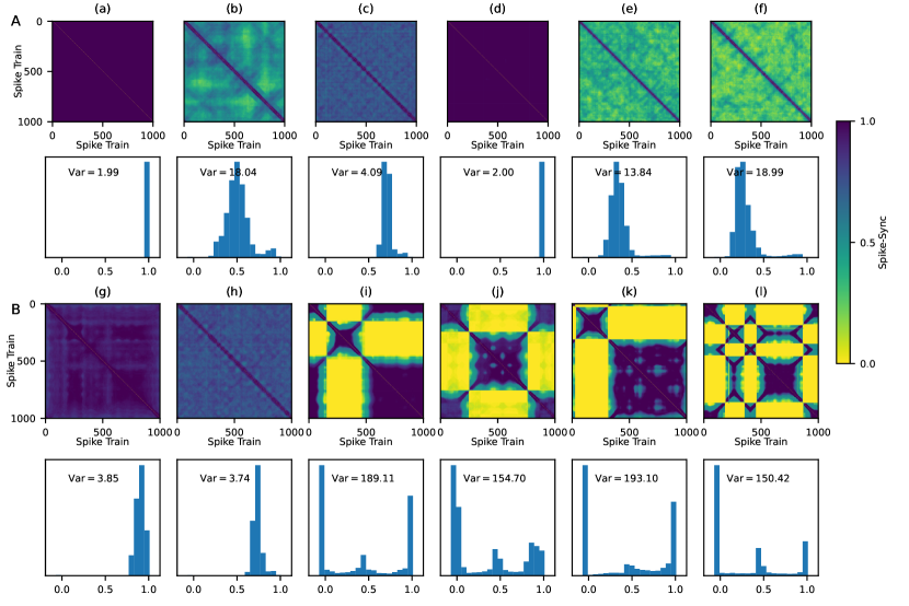
Figure 5: Dissimilarity matrices obtained by pairwise spike-sync of the spike trains of excitatory population. A and B, top: SPIKE-sync matrices obtained at different values of synaptic noise strength $g_{sE}$ in balanced neuronal networks of hybrid synaptic connections. Below each matrix, an histogram of the spike-syn values is shown. Values of Variance, Var ( = Variance*1000), are shown inside each histogram plot. A. $J_{EE}=0.5$ ; B. $J_{EE}=1.5$ .

To demonstrate groups (or clusters) as well as transitions of various firing pattern that already observed, dissimilarity matrices obtained by pairwise spike-sync in Eq.9 have been introduced. Dissimilarity matrices (Fig.5) show distinctive patterns for the unsynchronized and synchronized situations at two different level of excitatory strength.In the first case of higher correlated state, complete (Fig.5(a),(d)) and moderate synchronous state (Fig.5(c),(g),(h)) have been clearly detected depending on values outside the diagonal and their variances. On the other hand, for complete synchronous state, all the values in the dissimilarity matrix are equal to 1, meaning that the synchronization is the same and maintained through all the simulation; for moderate synchronous state, dissimilarity matrices show a mixture of values between 0.5 and 1, that evidence a lower degree of synchrony firing patterns. In the second case of uncorrelated state, asychronous firing state and multistable state have already been observed. For weaker excitatory connections (shown in Fig.5A), dissimilarity matrices with smaller $g_{sE}$ show intermediate values around 0.5, that imply a coexisting firing patterns of multistable regime as a transition between complete and moderate synchronous state shown in Fig.5(b). Moreover, at the large $g_{sE}$, values in dissimilarity matrices are almostly less than 0.5 and the mean of SPIKE-Syn is around 0.25 , that are asychronous firing state shown in Fig.5(e),(f). However, for a little stronger excitatory connections (see Fig.5B), dissimilarity matrices display some clusters of the values between 0 and 1 at the large $g_{sE}$ , with noticeable regular ‘patches’ shown in Fig.5(i) -(l) that evidence the maintenance of some synchronization patterns. The histograms of SPIKE-syn values (shown in Fig.5 below each dissimilarity matrice) are also useful in detecting the three situations described.

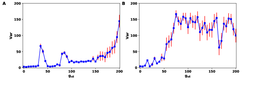
Figure 6: Variance of the SPIKE-Sync values (the same values plotted in the histograms) plotted against $g_{sE}$, where Var shown as ylabel is defined as: Var =Variance of SPIKE-Sync values*1000. Average (±SEM) of 10 simulations with different random seeds for the small-world connectivity and parameters.A. $J_{EE}=0.5$; B. $J_{EE}=1.5$.

As a rough measure of multistability, we took the variance of the SPIKE-Syn values (outside the diagonal) and plotted them against the strengths of synaptic noise, averaging several simulations with different seed for the random connectivity matrix(Fig.6). Var is $0$ if the system is either completely synchronized or completely desynchronized and a high value is present only when periods of coherence alternate with periods of incoherence. At weak excitatory coupling (Fig.6LABEL:Fig7VariA), it is clear that the neuronal networks can produce time-varying coexisting firing patterns of that Var $>$0, which is investigated and shown in Fig.3 , for some suitable values of $g_{sE}$. Besides, transitions between different neuronal firing patterns are clearly exhibited with varying $g_{sE}$. With high level of excitatory coupling (Fig.6B), both time-varying and parameter-varying coexisting firing patterns have been clearly observed in a wider $g_{sE}$ range, particular when $g_{sE}\geq 50$ of Var $>>$0. Overall, the SPIKE-Syn values with signatures of coexisting firing activies confirms again that multistable behaviour are more easily obtained when the networks are at different level of excitatory coupling, while parameter-varying coexistence of synchrony and various ripple events are more easily observed when the networks are at high level excitatory coupling.

V Effect of excitatory coupling strengths in the generation of coexisting dynamical regimes

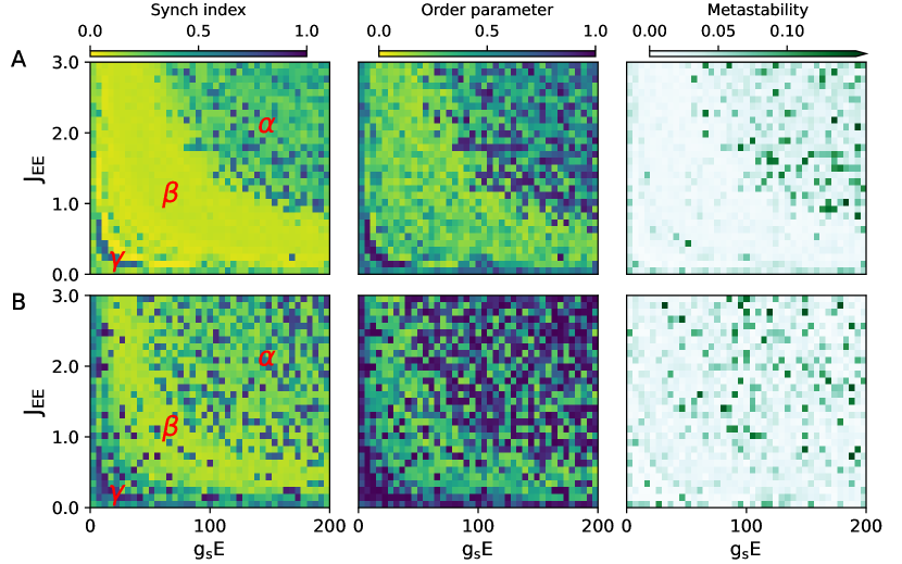
Figure 7: The influence of excitatory synaptic weights on coexisting firing patterns in $g_{sE}/{J_{EE}}$ parameter space at two different level of electrical coupling. Regions $\alpha$ and $\gamma$ denote coexisting firing patterns, showing the similar dynamical behaviour that observed in Fig.2.Region $\beta$ exhibits asychronous firing state with lower values ($\approx 0$) of statistical parameters. Weights of electrical synaptic coupling are: A.$J_{gap}=0.1$ ; B.$J_{gap}=1$.

To present a broader perspective on variety of firing patterns that affected by combination of chemical synaptic noise and strengths of excitatory connections, we explore the synchronized and asynchronized states as well as coexisting firing patterns in $g_{sE}/{J_{EE}}$ parameter space. Fig.7A,B shows the collective behavior of excitatory neurons at two different level of electrical coupling, respectively. With weak electrical synaptic coupling of that $J_{gap}=0.1$, it is clear that both asynchronized states (green- yellow region, $\beta$) and ’speckle’ pattern of coexisting firing state (regions $\alpha$ and $\gamma$) have been observed with sweeping $g_{sE}/J_{EE}$ shown in Fig.7A(left). Moreover, coexisting firing patterns of interest induced by synaptic noise separates into two distributaries (regions $\alpha$ and $\gamma$) through asynchronized firing state of region $\beta$. In other words, the asynchronized firing regimes emerges as a transition among coexisting firing state shown in Fig.7A(left).The results of these finding also has been evidenced by a statistical methods of order parameter and metstability shown in the Fig.7A(middle and right). However, in the case of stronge electrical synaptic coupling when $J_{gap}=1$, Fig.7B exhibits that asychronous firing regimes have been gradually displaced by coexisting firing patterns,that will cover the overall $g_{sE}/J_{EE}$ parameter space eventually with further increasing electrical synaptic weights. At end, our findings imply that synaptic noise, excitatory synaptic weights as well as electrical coupling strengths make a significant contribution to the generation of coexisting firing patterns in the hybrid synaptic interacting balanced neuronal network.

In summery, we investigated multistability or coexistence of neural firing pattens that driven by chemical synaptic noise in a balanced network of excitatory neurons connected by hybrid synapses. Using statistical measurement of synch-index, order parameter , metastability and SPIKE-syn, we found that strengths of synaptic noise and excitatory weights make a greater contribution than variance of synaptic noise to the coexistence of firing states with slight modification parameters. Specifically, the coexisting firing patterns in a hydrid coupling neural networks can emerge in two ways, including time-varying and parameter-varying coexisting firing patterns. The first type of coexisting firing patterns in neural systems is typically metstable state as format of the time-varying coexistence, namely coexistence or alternation of synchronous state and traveling wave. The presence of this coexistence firing patterns has been observed under the fixed combination of synaptic noise strengths and excitatory connection weights. The second type of multistability in neural networks is parameter-varying coexistence. The parameter-varying coexistence is accompanied by coexistence of coherence(synchrony state) and incoherence firing state(metastable or asynchronous firing pattern) with slightly varying control parameters.

VI summery and discussion

The phenomenon of multistability has been found in various classes of dynamical systems such as delayed feedback systems,weakly coupled systems, excited systems, and stochastic systems[32, 33].The appearance of multistability depends on many factors such as the strength of dissipation,the nature and strength of coupling, the value of the time delay, amplitude and frequency of the parameter perturbation,and noise intensity[1, 6]. Experiments as well as theoretical models have revealed different routes to multistability in the different system classes(see review[1]).In previous works[4, 20] and in the present one, we try to unveil the impact of synaptic connections as well as the node dynamics to the various firing activities and the multistable dynamics found in a hybrid synaptic interacting balanced neuronal network.

A wealth of evidence indicates abundant electrical synapses interlinking excitatory neurons.Electrical synapses occur between excitatory glutamatergic inferior olivary cells [34], glutamatergic excitatory trigeminal mesencephalic primary afferent neurons[35], and others(reviewed in[36]).Nevertheless,theoretical understanding of hybrid synaptic connections in diverse dynamical states of neural networks for self-organization and robustness still has not been fully studied. In order to reveal the underlying roles of this mixed synaptic connection on various firing patterns, we have already presented a model of neural network including chemical excitatory and electrical synaptic coupling for excitatory population in our previous work[20]. In this balanced neural networks, we found that the emergence of various firing ripple events has been observed by considering the variation of chemical synaptic inhibition and network densities. Secondly, we also can see that the excitatory population has a tendency to synchronization as the weights of electrical synaptic coupling among excitatory cells are increased. Moreover, the existence of this mixed synaptic connections in excitatory population can cause various firing patterns of interest by slightly changing the chemical synaptic weights. As we know, observation of neural noise has been explored in multiple experimental studies from the perception of sensory signals to the generation of motor responses[8, 9]. However, effect of synaptic noise on genertion of coexisting firing patterns in a hybrid connected balanced networks has not well been considered in that study.

It is generally accepted that coexisting firing patterns induced by noise or chaos can arise in networks purely connected by electrical or chemical synapses together with synaptic weights and seems to depend on other factors such as time delay and networks topology[37, 38]. Computational models show promise to identify some of underlying mechanisms to reproduce coexisting firing patterns. Early studies have reported that the inclusion of noise was regarded as an ad hoc mechanism required to produce interesting dynamics[39, 40, 41, 42]. A common feature of the noise-driven multistable models is the existence of a subcritical Hopf bifurcation to generate multiple attractors. Then, noise produces the switching between them. In other words, for deterministic models attracted to stable or periodic solutions, noise is fundamental to avoid that dynamics become stuck in a state of equilibrium. Therefore, the ad hoc introduction of noise in a dynamical system near a bifurcation ensures stochastic switching between different attractors, endowing the simulation with the kind of various firing patterns seen in the empirical data.

Some other researchers have already explored deterministic chaos as an alternative to noise-induced multistability to reproduce statistical observables computed from experiment recordings. It is well known that chaos has a key feature of highly dependent on the initial conditions[43]. Chaotic itinerancy and heteroclinic cycling talk about deterministic dynamics[44, 15],endowing networked chaotic dynamical systems with complex metastable dynamics in the absence of noise. Previous studies demonstrated that chaos can emerge in medium or large size neural networks[45, 46] and even in small circuits or low-dimension mean-field approximations[47, 18]. Some others studies also showed that neuronal activity is intrinsically irregular in the generation of action potentials, their axonal propagation, and the synaptic transmission that follows[8, 48]. Therefore, both deterministic and stochastic mechanisms are present in neural dynamics and they should contribute differently to the functional connectivity dynamics. In all, many advances have been made to understand how network topology, connection delays, and noise can contribute to building this dynamic. Little or no attention, however, has been paid to the difference between local chaotic and stochastic influences on the switching between different network states.

More recent has seen a growing body of modelling studies on the comparation and contribution of chaos and noise to multistable dynamics of neural network. Some earlier studies have explored multistable dynamics of networks composed by chaotic oscillators without noise at all[49, 50], and others have used simple oscillatory or non-oscillatory nodes of their dynamics driven by noise[41, 51].After that, some works employ complex dynamic models at the node level but still in presence of neural noise to drive the multistability[52, 53, 39, 54]. Finally, recent studies have begun to explore the significant difference mechanisms of neural noise and deterministic chaos to drive multistability[4, 5]. Piccinini et al.[5] showed that chaotic dynamics give rise to some interesting features in whole-brain activity models, out performing noise-driven equilibrium models in the simultaneous reproduction of multiple empirical observables.

Our previous study have shown how channel noise can alter the multistable dynamics that is induced by chaos in a weakly coupled,heterogeneous, network of neural oscillators[4].Using a conductance-based neural model that can have chaotic dynamics, we found that a network can show multistable dynamics in a certain range of global connectivity strength and under deterministic conditions. We characterized the multistable dynamics when the networks are, in addition to chaotic, subject to ion channel stochasticity in the form of multiplicative (channel) or additive (current) noise. More importanly, results of our previous work shown that moderate noise can enhance the multistable behavior that is evoked by chaos, resulting in more heterogeneous synchronization patterns, while more intense noise abolishes multistability.

At first glance, our results are not as straightforward to interpret as in the previously mentioned works. With the goal of understanding what role of synaptic noise between excitatory cells might play in influencing collective neural dynamics, we systematically swept the parameters of synaptic noise and excitatory coupling weights, trying to keep other variables, such as parameters of synaptic dynamics. In this paper, we show that both synaptic noise intensity and excitatory weights can make a great contribution to the coexistence of firing states with slight modification parameters. First, we find that neuronal networks can display time-varying and parameter-varying multistability. Second, we also find that the emergence of time-varying multistability is shown as a format of metstable state, while the parameter-varying multistability is accompanied by coexistence of synchrony state and metastable (or asynchronous firing state) with slightly varying noise intensity and excitatory weights. Our results offer a series of precise statistical explanation of the intricate effect of synaptic noise in neural multistability.

Our findings have some issues that need to be considered when interpreting them.We are studying multistability in a medium-sized network of oscillatory neurons and trying to relate its behavior to phenomena observed at much larger scales. The main difference, which was also explained in previous study[4], between our model and large scale ones is the nature of synaptic connections between neurons. In our previous studies[55, 56, 18, 4, 20, 57, 58], we first have used electrical synapses[18, 4, 57, 58],a type of bidirectional synapse that has a dampening effect with a natural tendency to synchronize a network, while long-range connections in the brain are unidirectional with chemical synaptic nature. This type of connection generates more complex dynamics, especially when time delays and noise are considered[59]. Chemical synaptic coupling is responsible for a variety of network effects, particularly in networks that generate rhythmic activity some of which are well established, such as regulation of phase relationships[55, 56], synchrony[60, 61], and pattern formation[20], and some are novel, such as coexistence of firing patterns driven by chaos or noise. Recently, many experiments have evidenced that diverse neural circuits use hybrid synapses coexisting in most organisms and brain structures, the precise mechanisms whereby these hybrid synapses contribute to various firing modes of brain activities are subtle and remain elusive. On the other hand, electrical synapses are localized primarily in inhibitory neurons widely distributed throughout the CNS, whereas we here presente a model of electrical synapses interlinking excitatory neurons[34, 35, 36].

Brain dynamics is often inherently variable and unstable, consisting of sequences of transient spatiotemporal patterns[38, 62]. These sequences of transients are a hallmark of metastable dynamics that are neither entirely stable nor completely unstable. The neuronal noise of brain dynamics, given by synaptic connections and channel noise, must play a role in the observed multistable dynamics. Here we present the first attempt to raise the question and find two types of coexisting firing patterns.Our results pave a possible way to uncover the underlying mechanisms of noise-driven coexisting firing patterns, such as metastable dynamics, that may mediate perception and cognition.

Appendix A

1. Parameters and functions of Wang-Buzsáki model

   $g_{L}=0.1$	$g_{Na}=35$	$g_{K}=9$ ($mS/cm^{2}$)
   $E_{L}=-65$	$E_{Na}=55$	$E_{K}=-90$ (mV)
   $C_{m}=1$ ($\mu F)$	$\phi=5$	$I_{app}=0$ ($\mu A/cm^{2}$)

   $\alpha_{m}(V)=-0.1(V+35)/[exp(-0.1(V+35))+1]$	$\beta_{m}(V)=4exp[-(V+60)/18]$
   $\alpha_{h}(V)=0.07exp[-(V+58)/20]$	$\beta_{h}(V)=1/exp[-0.1(V+28)]+1$
   $\alpha_{n}(V)=-0.01(V+34)/[exp(-0.1(V+34))-1]$	$\beta_{n}(V)=0.125exp[-(V+44)/80]$
   $m_{\infty}=\alpha_{m}/(\alpha_{m}+\beta_{m})$

   Table 1: Parameters and functions of Wang-Buzsáki model(1996)[19]

2. The updating rule of chemical synaptic conductances

   In simulations and for practical reasons, the updating rule of chemical synaptic conductances is the same as our previous study[20], following :

   $$\frac{dy}{dt} ={\bar{g}}_{s(E,I,\nu)}f\delta\left(t_{0}+t_{d}-t\right)-\left(\frac{1}{\tau_{1}}+\frac{1}{\tau_{2}}\right)y-\frac{g_{syn}}{\tau_{1}\tau_{2}}$$

   $$\frac{dg_{syn}}{dt} =y$$ (10)

   

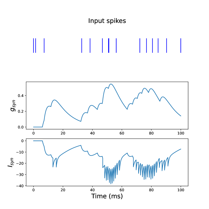
   Figure 8: Time course of excitatory synaptic input. Top. presynaptic (input) spikes; Middle.the time course of the synaptic conductance, $g_{syn}$, activated by input spikes; Bottom.excitatory postsynaptic currents (EPSPs) caused by the simultaneous activation of synapses.

   The delta function $\delta\left(t_{0}+t_{d}-t\right)$ represents the spike signal from presynatpic cell, that is $1$ when $t=t_{0}+t_{d}$ and 0 otherwise. The time $t_{0}$ is the time of the presynaptic spike and $t_{d}$ is synaptic delays from the presynatpic to postsynaptic cell. The conductance peaks occurs at time $t_{peak}=t_{0}+t_{d}+\frac{\tau_{1}\tau_{2}}{\tau_{1}-\tau_{2}}ln(\tau_{1}/\tau_{2})$. The normalization factor $f=1/(e^{-t_{peak}/\tau_{1}}-e^{-t_{peak}/\tau_{2}})$ and $t_{peak}=\frac{\tau_{1}\tau_{2}}{\tau_{1}-\tau_{2}}ln(\tau_{1}/\tau_{2})$, ensure that the maximum amplitude of the impulse response equals ${\bar{g}}_{s(E,I,\nu)}$. The example of time course of synaptic conductance and excitatory synaptic currents activated by input spikes are shown in Fig.8 In simulations of this work, both peak synaptic conductances ${\bar{g}}_{s(E,I,\nu)}$ and synaptic delays $t_{d}$ are Gaussian distributed random variables with prescribed means $g_{s(E,I)}$ and $\overline{D}$, and standard deviation $\sigma_{g_{s(E,I)}}$ and $\sigma_{\overline{D}}$. The background drive $v_{ext}$ to each neuron in the excitatory population was provided by external excitatory inputs, modeled as independent and identically distributed Poisson processes with rate $\nu$ for different neurons. Peak conductances of the external drive were also heterogeneous and assumed values sampled from a truncated Gaussian distribution with mean $g_{s\nu}$ and standard deviation $\sigma_{g_{s\nu}}$. These rules are the same as our previous study[20]. Parameters of synaptic model are summarized in Table 2.

3. List of simulation and default network parameters in the E/I balanced networks

   A: Global simulation paramters
   Description	Symbol	Value
   Simulation duration	$T_{sim}$	2000 ms
   Start-up transient	$T_{trans}$	400 ms
   Time step	dt	0.02 ms
   B: Populations and external input
   Description	Symbol	Value
   Population size of excitatory neurons	$N_{E}$	1000
   Population size of inhibitory neurons	$N_{I}$	250
   Possion input rate (external excitatory inputs)	$\nu$	6000 Hz
   C: Connection parameters
   Description	Symbol	Value
   Weight of gap junction	$J_{gap}$	0.1
   Weight of self-excitatory connection	$J_{EE}$	0.05
   Weight of self-inhibitory connection	$J_{II}$	0.04
   Weight of inhibitory connections for excitatory population	$J_{EI}$	0.03
   Weight of excitatory connections for inhibitory population	$J_{IE}$	0.01
   Probability of local inhibitory connections	$P_{I}$	0.2
   Synaptic dynamics (Difference of Two Exponentials)
   Reversal potential for excitatory synapses	$E_{synE}$	0 mV
   Reversal potential for inhibitory synapses	$E_{synI}$	-80 mV
   Excitatory synaptic decay time	$\tau_{1E}$	3 ms
   Ihibitory synaptic decay time	$\tau_{1I}$	4 ms
   Excitatory synaptic time	$\tau_{2E}$	1 ms
   Inhibitory synaptic time	$\tau_{2I}$	1 ms
   Mean synaptic delay	$\overline{D}$	1.5 ms
   Mean synaptic excitatory conductance	$g_{sE}$	5 nS
   Mean synaptic inhibitory conductance	$g_{sI}$	200 nS
   Mean synaptic input conductance	$g_{s\nu}$	3 nS
   Standard deviation delay	$\sigma_{\overline{D}}$	0.1 ms
   Standard synaptic excitatory conductance	$\sigma_{g_{sE}}$	1 nS
   Standard inhibitory conductance	$\sigma_{g_{sI}}$	10 nS
   Standard input conductance	$\sigma_{g_{s\nu}}$	1 nS
   Small-world networks (SW)
   Probability of replacing new links	$P_{sw}$	0.01
   Degree of nearest neighbours connections	K	10

   Table 2: List of simulation and default network parameters in the E/I balanced networks.

References

- Pisarchik and Feudel [2014] A. N. Pisarchik and U. Feudel, Control of multistability, Physics Reports 540, 167 (2014).
- Cole et al. [2016] M. W. Cole, T. Ito, D. S. Bassett, and D. H. Schultz, Activity flow over resting-state networks shapes cognitive task activations, Nature neuroscience 19, 1718 (2016).
- Chopek et al. [2019] J. W. Chopek, H. Hultborn, and R. M. Brownstone, Multistable properties of human subthalamic nucleus neurons in parkinson’s disease, Proceedings of the National Academy of Sciences 116, 24326 (2019).
- Orio et al. [2018] P. Orio, M. Gatica, R. Herzog, J. P. Maidana, S. Castro, and K. Xu, Chaos versus noise as drivers of multistability in neural networks, Chaos: An Interdisciplinary Journal of Nonlinear Science 28, 106321 (2018).
- Piccinini et al. [2021] J. Piccinini, I. P. Ipiñna, H. Laufs, M. Kringelbach, G. Deco, Y. Sanz Perl, and E. Tagliazucchi, Noise-driven multistability vs deterministic chaos in phenomenological semi-empirical models of whole-brain activity, Chaos: An Interdisciplinary Journal of Nonlinear Science 31, 023127 (2021).
- Kim et al. [1997] S. Kim, S. H. Park, and C. Ryu, Multistability in coupled oscillator systems with time delay, Physical review letters 79, 2911 (1997).
- Buceta and Lindenberg [2004] J. Buceta and K. Lindenberg, Comprehensive study of phase transitions in relaxational systems with field-dependent coefficients, Physical Review E 69, 011102 (2004).
- Faisal et al. [2008] A. A. Faisal, L. P. Selen, and D. M. Wolpert, Noise in the nervous system, Nature reviews neuroscience 9, 292 (2008).
- McDonnell and Ward [2011] M. D. McDonnell and L. M. Ward, The benefits of noise in neural systems: bridging theory and experiment, Nature Reviews Neuroscience 12, 415 (2011).
- Lillywhite and Laughlin [1979] P. Lillywhite and S. Laughlin, Transducer noise in a photoreceptor, Nature 277, 569 (1979).
- Rusakov et al. [2020] D. A. Rusakov, L. P. Savtchenko, and P. E. Latham, Noisy synaptic conductance: bug or a feature?, Trends in Neurosciences 43, 363 (2020).
- Hamilton et al. [2004] A. F. d. C. Hamilton, K. E. Jones, and D. M. Wolpert, The scaling of motor noise with muscle strength and motor unit number in humans, Experimental brain research 157, 417 (2004).
- Anderson et al. [2000] J. S. Anderson, I. Lampl, D. C. Gillespie, and D. Ferster, The contribution of noise to contrast invariance of orientation tuning in cat visual cortex, Science 290, 1968 (2000).
- Stocks [2000] N. G. Stocks, Suprathreshold stochastic resonance in multilevel threshold systems, Physical Review Letters 84, 2310 (2000).
- Miller [2016] P. Miller, Itinerancy between attractor states in neural systems, Current opinion in neurobiology 40, 14 (2016).
- Tang et al. [2011] G. Tang, K. Xu, and L. Jiang, Synchronization in a chaotic neural network with time delay depending on the spatial distance between neurons, Physical Review E 84, 046207 (2011).
- Xu et al. [2017] K. Xu, J. P. Maidana, M. Caviedes, D. Quero, P. Aguirre, and P. Orio, Hyperpolarization-activated current induces period-doubling cascades and chaos in a cold thermoreceptor model, Frontiers in computational neuroscience 11, 12 (2017).
- Xu et al. [2018] K. Xu, J. P. Maidana, S. Castro, and P. Orio, Synchronization transition in neuronal networks composed of chaotic or non-chaotic oscillators, Scientific reports 8, 1 (2018).
- Wang and Buzsáki [1996] X.-J. Wang and G. Buzsáki, Gamma oscillation by synaptic inhibition in a hippocampal interneuronal network model, Journal of neuroscience 16, 6402 (1996).
- Xu et al. [2021] K. Xu, J. P. Maidana, and P. Orio, Diversity of neuronal activity is provided by hybrid synapses, Nonlinear Dynamics 105, 2693 (2021).
- Calim et al. [2018] A. Calim, P. Hövel, M. Ozer, and M. Uzuntarla, Chimera states in networks of type-i morris-lecar neurons, Physical Review E 98, 062217 (2018).
- Hodgkin and Huxley [1952] A. L. Hodgkin and A. F. Huxley, A quantitative description of membrane current and its application to conduction and excitation in nerve, The Journal of physiology 117, 500 (1952).
- Izhikevich [2007] E. M. Izhikevich, Dynamical systems in neuroscience (MIT press, 2007).
- Laing and Lord [2009] C. Laing and G. J. Lord, Stochastic methods in neuroscience (OUP Oxford, 2009).
- Watts and Strogatz [1998] D. J. Watts and S. H. Strogatz, Collective dynamics of ’small-world’ networks, Nature 393, 440 (1998).
- Golomb and Rinzel [1993] D. Golomb and J. Rinzel, Dynamics of globally coupled inhibitory neurons with heterogeneity, Physical review E 48, 4810 (1993).
- Kuramoto [2003] Y. Kuramoto, Chemical oscillations, waves, and turbulence (Courier Corporation, 2003).
- Bertolotti et al. [2017] E. Bertolotti, R. Burioni, M. di Volo, and A. Vezzani, Synchronization and long-time memory in neural networks with inhibitory hubs and synaptic plasticity, Physical Review E 95, 012308 (2017).
- Shanahan [2010] M. Shanahan, Metastable chimera states in community-structured oscillator networks, Chaos: An Interdisciplinary Journal of Nonlinear Science 20, 013108 (2010).
- Kreuz et al. [2015] T. Kreuz, M. Mulansky, and N. Bozanic, Spiky: a graphical user interface for monitoring spike train synchrony, Journal of neurophysiology 113, 3432 (2015).
- Mulansky and Kreuz [2016] M. Mulansky and T. Kreuz, Pyspike—a python library for analyzing spike train synchrony, SoftwareX 5, 183 (2016).
- Feudel [2008] U. Feudel, Complex dynamics in multistable systems, International Journal of Bifurcation and Chaos 18, 1607 (2008).
- Stankovski et al. [2017] T. Stankovski, T. Pereira, P. V. McClintock, and A. Stefanovska, Coupling functions: universal insights into dynamical interaction mechanisms, Reviews of Modern Physics 89, 045001 (2017).
- Llinas et al. [1974] R. Llinas, R. Baker, and C. Sotelo, Electrotonic coupling between neurons in cat inferior olive., Journal of neurophysiology 37, 560 (1974).
- Hinrichsen [1970] C. Hinrichsen, Coupling between cells of the trigeminal mesencephalic nucleus, Journal of dental research 49, 1369 (1970).
- Nagy et al. [2018] J. I. Nagy, A. E. Pereda, and J. E. Rash, Electrical synapses in mammalian cns: Past eras, present focus and future directions, Biochimica Et Biophysica Acta (BBA)-Biomembranes 1860, 102 (2018).
- Baptista et al. [2010] M. Baptista, F. M. Kakmeni, and C. Grebogi, Combined effect of chemical and electrical synapses in hindmarsh-rose neural networks on synchronization and the rate of information, Physical Review E 82, 036203 (2010).
- Sporns [2010] O. Sporns, Networks of the brain. masachusettes (2010).
- Deco and Jirsa [2012] G. Deco and V. K. Jirsa, Ongoing cortical activity at rest: criticality, multistability, and ghost attractors, Journal of Neuroscience 32, 3366 (2012).
- Golos et al. [2015] M. Golos, V. Jirsa, and E. Daucé, Multistability in large scale models of brain activity, PLoS computational biology 11, e1004644 (2015).
- Hansen et al. [2015] E. C. Hansen, D. Battaglia, A. Spiegler, G. Deco, and V. K. Jirsa, Functional connectivity dynamics: modeling the switching behavior of the resting state, Neuroimage 105, 525 (2015).
- Deco et al. [2017a] G. Deco, M. Kringelbach, V. Jirsa, and P. Ritter, The dynamics of resting fluctuations in the brain: metastability and its dynamical cortical core. sci. rep. 7, 3095 (2017a).
- Strogatz [2018] S. H. Strogatz, Nonlinear dynamics and chaos: with applications to physics, biology, chemistry, and engineering (CRC press, 2018).
- Friston et al. [2012] K. Friston, M. Breakspear, and G. Deco, Perception and self-organized instability, Frontiers in computational neuroscience 6, 44 (2012).
- Sompolinsky et al. [1988] H. Sompolinsky, A. Crisanti, and H.-J. Sommers, Chaos in random neural networks, Physical review letters 61, 259 (1988).
- Sprott [2008] J. Sprott, Chaotic dynamics on large networks, Chaos: An Interdisciplinary Journal of Nonlinear Science 18, 023135 (2008).
- Fasoli et al. [2016] D. Fasoli, A. Cattani, and S. Panzeri, The complexity of dynamics in small neural circuits, PLoS computational biology 12, e1004992 (2016).
- Faisal et al. [2005] A. A. Faisal, J. A. White, and S. B. Laughlin, Ion-channel noise places limits on the miniaturization of the brain’s wiring, Current Biology 15, 1143 (2005).
- Honey et al. [2007] C. J. Honey, R. Kötter, M. Breakspear, and O. Sporns, Network structure of cerebral cortex shapes functional connectivity on multiple time scales, Proceedings of the National Academy of Sciences 104, 10240 (2007).
- Gollo and Breakspear [2014] L. L. Gollo and M. Breakspear, The frustrated brain: from dynamics on motifs to communities and networks, Philosophical Transactions of the Royal Society B: Biological Sciences 369, 20130532 (2014).
- Deco et al. [2017b] G. Deco, J. Cabral, M. W. Woolrich, A. B. Stevner, T. J. Van Hartevelt, and M. L. Kringelbach, Single or multiple frequency generators in on-going brain activity: A mechanistic whole-brain model of empirical meg data, Neuroimage 152, 538 (2017b).
- Pototsky [2012] A. Pototsky, Emergence and multistability of time-periodic states in a population of noisy passive rotators with time-lag coupling, Physical Review E 85, 036219 (2012).
- Deco et al. [2013] G. Deco, A. Ponce-Alvarez, D. Mantini, G. L. Romani, P. Hagmann, and M. Corbetta, Resting-state functional connectivity emerges from structurally and dynamically shaped slow linear fluctuations, Journal of Neuroscience 33, 11239 (2013).
- Freyer et al. [2011] F. Freyer, J. A. Roberts, R. Becker, P. A. Robinson, P. Ritter, and M. Breakspear, Biophysical mechanisms of multistability in resting-state cortical rhythms, Journal of Neuroscience 31, 6353 (2011).
- Xu et al. [2013] K. Xu, W. Huang, B. Li, M. Dhamala, and Z. Liu, Controlling self-sustained spiking activity by adding or removing one network link, EPL (Europhysics Letters) 102, 50002 (2013).
- Xu et al. [2014] K. Xu, X. Zhang, C. Wang, and Z. Liu, A simplified memory network model based on pattern formations, Scientific reports 4, 1 (2014).
- Tian et al. [2018] C. Tian, L. Cao, H. Bi, K. Xu, and Z. Liu, Chimera states in neuronal networks with time delay and electromagnetic induction, Nonlinear Dynamics 93, 1695 (2018).
- Zhou et al. [2021] J.-F. Zhou, E.-H. Jiang, B.-L. Xu, K. Xu, C. Zhou, and W.-J. Yuan, Synaptic changes modulate spontaneous transitions between tonic and bursting neural activities in coupled hindmarsh-rose neurons, Physical Review E 104, 054407 (2021).
- Deco et al. [2009] G. Deco, V. Jirsa, A. R. McIntosh, O. Sporns, and R. Kötter, Key role of coupling, delay, and noise in resting brain fluctuations, Proceedings of the National Academy of Sciences 106, 10302 (2009).
- Ashhad and Feldman [2020] S. Ashhad and J. L. Feldman, Emergent elements of inspiratory rhythmogenesis: network synchronization and synchrony propagation, Neuron 106, 482 (2020).
- Montbrió and Pazó [2020] E. Montbrió and D. Pazó, Exact mean-field theory explains the dual role of electrical synapses in collective synchronization, Physical Review Letters 125, 248101 (2020).
- Rabinovich et al. [2008] M. I. Rabinovich, R. Huerta, P. Varona, and V. S. Afraimovich, Transient cognitive dynamics, metastability, and decision making, PLoS computational biology 4, e1000072 (2008).