Multihop Optical Wireless Communication Over ${\cal{F}}$-Turbulence Channels and Generalized Pointing Errors with Fog-Induced Fading

Abstract

Multihop relaying is a potential technique to mitigate channel impairments in optical wireless communications (OWC). In this paper, multiple fixed-gain amplify-and-forward (AF) relays are employed to enhance the OWC performance under the combined effect of atmospheric turbulence, pointing errors, and fog. We consider a long-range OWC link by modeling the atmospheric turbulence by the Fisher-Snedecor ${\cal{F}}$ distribution, pointing errors by the generalized non-zero boresight model, and random path loss due to fog. We also consider a short-range OWC system by ignoring the impact of atmospheric turbulence. We derive novel upper bounds on the probability density function (PDF) and cumulative distribution function (CDF) of the end-to-end signal-to-noise ratio (SNR) for both short and long-range multihop OWC systems by developing exact statistical results for a single-hop OWC system under the combined effect of ${\cal{F}}$-turbulence channels, non-zero boresight pointing errors, and fog-induced fading. Based on these expressions, we present analytical expressions of outage probability (OP) and average bit-error-rate (ABER) performance for the considered OWC systems involving single-variate Fox’s H and Meijer’s G functions. Moreover, asymptotic expressions of the outage probability in high SNR region are developed using simpler Gamma functions to provide insights on the effect of channel and system parameters. The derived analytical expressions are validated through Monte-Carlo simulations, and the scaling of the OWC performance with the number of relay nodes is demonstrated with a comparison to the single-hop transmission.

TABLE I: Related literature on AF-assisted multihop OWC systems

Reference	Detector	Turbulence	Pointing Errors	Fog-Induced Fading
[9]	IM/DD	Gamma-Gamma	No	No
[18]	IM/DD	Gamma-Gamma	No	No
[19]	IM/DD	Gamma-Gamma	Zero boresight	No
[20]	HD	Gamma-Gamma	Zero boresight	No
[21]	HD	Gamma-Gamma	Zero boresight	No
[22]	IM/DD	Malága	Zero boresight	No
[23]	HD	Malága	Zero boresight	No
[26]	IM/DD	Double Generalized Gamma	Zero boresight	No
[This paper]	IM/DD	Fisher-Snedecor ${\cal{F}}$	Non-zero boresight	Yes

TABLE II: Related literature on OWC systems with Fog-induced fading

Reference	System Model	Pointing Errors	Turbulence
[34]	Single-hop	No	No
[35]	Single-hop	No	No
[46]	Single-hop	No	No
[37]	Single-hop	Zero boresight	No
[42]	Single-hop	Zero boresight	Fisher-Snedecor ${\cal{F}}$
[38]	Dual-hop, DF	Zero boresight	Double Generalized Gamma
[36]	Multihop, DF	Zero boresight	No
[This paper]	Single and Multihop, AF	Non-zero boresight	Fisher-Snedecor ${\cal{F}}$

I Introduction

Optical wireless communication (OWC) is emerging as a key technology for backhaul connectivity in the next-generation wireless network [1, 2, 3, 4]. The OWC system exploits large unlicensed bandwidth to provide exceedingly higher data rate with low latency transmissions and possesses narrow beam divergence for secured data links without electromagnetic interference. Despite these advantages, the OWC technology is susceptible to atmospheric conditions such as turbulence environment and foggy weather conditions and requires line-of-sight prorogation with near-perfect beam-alignment between the transmitter and detector. Developing efficient techniques to mitigate these channel fading impairments efficiently is desirable for an effective design of OWC systems.

Multi-aperture and cooperative relaying are potential techniques to mitigate the fading effect and extend the communication range. There has been extensive research on relay-assisted OWC systems with regenerative and non-regenerative protocols under the combined effect of atmospheric turbulence and pointing errors. Dual-hop relaying using both decode-and-forward (DF) and amplify-and-forward (AF) protocols is a well-studied topic for optical wireless channels [5, 6, 7, 8]. However, analyzing the performance of multihop relaying is challenging for mathematically complicated turbulence fading models, especially when the AF relaying is employed at each hop. It is known that analyzing DF-assisted multihop system is greatly simplified since the performance analysis decouples into each hop independently and thus requires statistical derivation of a single link [9, 10, 11, 12, 13, 14, 15, 16]. Further, the DF-based multihop requires channel state information (CSI) at each hop and becomes impractical when the number of hops increases beyond a certain limit.

Scanning the literature, there have been studies on the AF relaying for multihop OWC transmissions [9, 17, 18, 19, 20, 21, 22, 23, 24, 25]. Tsiftsis et al. analyzed the exact performance of multihop optical transmission over Gamma-Gamma atmospheric turbulence using channel-assisted AF relaying [9]. However, fixed-gain relaying is desirable due to a simpler implementation but analyzing its performance becomes intractable for many fading channels. To circumvent this, the end-to-end signal-to-noise ratio (SNR) of the fixed-gain multihop AF relaying is upper bounded as the product of SNR of individual links for tractable performance analysis. This approach was first considered in [26] to analyze the multihop relayed communication over Nakagami-m fading channels. Datsikas et al. analyzed the outage probability (OP) and average bit-error-rate (ABER) of an AF-assisted multihop system over Gamma-Gamma atmospheric turbulence without considering the impact of pointing errors [17]. Tang et al. extended the work presented in [17] considering the combined effect of pointing errors and Gamma-Gamma distributed atmospheric turbulence for the heterodyne OWC system [20]. Zedini and Alouini developed exact and asymptotic analysis for the OP, ABER, and ergodic capacity for an OWC system, pointing errors and atmospheric turbulence. Later, they extended the analysis presented in [19] for the intensity modulation/decision-directed (IM/DD) OWC system [18]. Alheadary et al. considered the misaligned generalized Malaga turbulence and developed ABER performance for the multihop heterodyne OWC system [22]. Ashrafzadeh et al. used the method of induction to develope and exact analysis for an AF-assisted multihop OWC system under the double generalized Gamma turbulence with pointing errors [24, 25].

In the above and related literature, we find a few research gaps in the study of the AF-assisted multihop OWC system, which need to be addressed. Firstly, the AF-assisted multihop transmission was limited to zero-boresight pointing errors and random jitter. The jitter is a random offset of the beam center at the detector plane, and the boresight is the fixed displacement between the center of the beam and the center of the detector [6]. The nonzero boresight model generalizes the effect of pointing errors on the OWC. Although the statistical analysis of nonzero boresight pointing errors for OWC system has been investigated extensively in the literature for single-link, dual-hop, and multi-aperture, it has not been addressed for the AF-assisted multihop transmission. Indeed, there are a few works on the impact of generalized pointing errors but for DF-assisted multihop systems [15, 16].

Secondly, adopted models for atmospheric turbulence were Gamma-Gamma, double generalized Gamma, and Malága distributions. These models are mathematically complicated by including Bessel and Meijer’s G-functions in their probability density functions (PDF). Recently, Peppas et al. proposed a new atmospheric turbulence model for OWC, called Fisher-Snedecor $\cal{F}$, which provides a better fit for experimental data for all turbulence conditions [27]. Further, the PDF of $\cal{F}$ turbulence is more mathematically tractable since it includes elementary functions. There has been an increased interest to analyze the performance of OWC over $\cal{F}$ turbulence [28, 29, 30, 31, 32]. However, no work has been reported even with the DF-assisted multihop OWC system considering the $\cal{F}$ atmospheric turbulence model.

Thirdly, signal attenuation for OWC transmissions is assumed to be deterministic and quantified using a visibility range, for example, less attenuation in haze and more loss of signal power in foggy conditions. However, recent measurement data confirm that the signal attenuation in foggy weather for terrestrial applications is not deterministic but follows a probabilistic model [33, 34, 35]. The authors in [36, 37] analyzed the single-link performance of the OWC system under the combined effect of fog and pointing errors. Esmail et al. analyzed the OP of a multihop relay system employing the DF protocol (using the cumulative distribution function (CDF) of the SNR for a single link) to mitigate the effect of fog and pointing errors [36]. In our previous work [38], we studied the DF-based dual-hop relaying for the OWC system under the combined effect of random fog, zero-boresight pointing errors, and atmospheric turbulence distributed according to the double generalized gamma. To the best of the authors’ knowledge, there are no analyses available for AF-assisted multihop OWC system under the effect of random fog, non-zero boresight pointing errors, and atmospheric turbulence. In Table I and Table II, we provide a summary of the state-of-the art research on the multihop OWC system and OWC system with fog-induced fading, respectively.

In this paper, we employ multiple fixed-gain relays in each hop to enhance the OWC performance under the combined effect of atmospheric turbulence, pointing errors, and fog. The major contributions of the proposed work are listed as follows:

• We analyze the end-to-end performance of a fixed-gain AF multihop relayed OWC system considering independent and non-identical (i.ni.d) fading channels in each hop distributed according to the combined statistics of ${\cal{F}}$-turbulence channels, non-zero boresight pointing errors, and fog-induced fading.

• We develop exact statistical results for the direct link of OWC system under the combined effect of atmospheric turbulence, pointing errors, and random fog. We also develop statistical results for a short-range OWC system by ignoring the impact of atmospheric turbulence.

• We derive novel upper bounds on the PDF and CDF of the end-to-end SNR for fixed gain assisted multihop relaying for both short and long-range OWC systems involving single-variate Fox’s H and Meijer’s G functions.

• We use the derived statistical results to analyze the OP and ABER performance for single-hop and multihop transmissions considering both short and long-range OWC systems.

• We develop diversity order of the considered system by deriving asymptotic expressions of the OP in high SNR region to provide insights on the design aspects of channel and system parameters.

• We use computer simulations to demonstrate the significance of multihop relaying for OWC systems to mitigate the channel impairment compared with the single-hop system.

Notations: $(\cdot)_{i}$ denotes the $i$-th hop and $(\cdot)_{N}$ denotes the $N$-hop system. We denote the expectation operator by $\mathbb{E}[\cdot]$, Gamma function by $\Gamma(a)=\int\limits_{0}^{\infty}t^{a-1}e^{-t}dt$, upper incomplete Gamma function by $\Gamma(a,t)=\int_{t}^{\infty}s^{a-1}e^{-s}ds$, Gaussian Q function by $Q(\gamma)=\frac{1}{\sqrt{2\pi}}\int_{\gamma}^{\infty}e^{-\frac{u^{2}}{2}}du$, Meijer’s G-function by $G_{p,q}^{m,n}\left[z\middle|\begin{matrix}(a_{k})_{k=1:p}\\ (b_{k})_{k=1:q}\end{matrix}\right]$, and the Fox’s H-function by $H_{p,q}^{m,n}\left[z\middle|\begin{matrix}(a_{k},A_{k})_{k=1:p}\\ (b_{k},B_{k})_{k=1:q}\end{matrix}\right]$.

The rest of this paper is organized as follows. Section II describes the channel models for fog, non-zero boresight pointing errors, and atmospheric turbulence for multihop OWC communication. In Sections III and IV, the performance of long and short-range OWC systems in terms of OP and ABER is presented, respectively. Numerical and simulation results are presented in Section V. Finally, we conclude the findings of this paper in Section VI.

II System Model

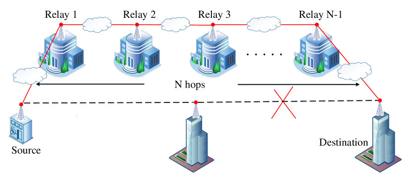
Figure 1: Multihop OWC communication system.

We consider an $N$-hop OWC system where a source terminal communicates with the destination through $N-1$ relay nodes. The transmitted signal is impaired by the multiplicative channel effects of atmospheric turbulence, pointing error, and random fog. Thus, the received signal $y_{i}$ for the $i$-th hop under the additive noise $w_{i}$ with variance $\sigma^{2}_{w_{i}}$ is given by

$$y_{i}=h_{i}s+w_{i},$$ (1)

where $s$ is the transmitted signal and $h_{i}=h_{f_{i}}h_{p_{i}}h_{t_{i}}$ is the channel coefficient of the $i$-th hop. Here, $h_{f_{i}}$ denotes the random fog, $h_{p_{i}}$ denotes the pointing error, $h_{t_{i}}$ denote the atmospheric turbulence. We use the simpler non-coherent intensity modulation/direct detection (IM/DD) scheme since heterodyne detection (HD) requires complex processing of mixing the received signal with a coherent signal produced by the local oscillator. Assuming IM/DD technique and on-off keying (OOK) modulation with $x\in\{0,\sqrt{2}P_{i}\}$ and $P_{i}$ as the average transmitted optical power, the instantaneous received electrical SNR for the $i$-th hop is given by [39]

$$\gamma_{i}^{\rm SH}=\frac{2P^{2}_{i}h_{i}^{2}}{\sigma^{2}_{w_{i}}}=\bar{\gamma}_{i}h_{i}^{2}$$ (2)

where $\bar{\gamma}_{i}$ is the average SNR of the $i$-th hop. Employing AF relaying with fixed-gain in each hop, the SNR of the $N$-th hop system is given by [40]:

$$\gamma_{\gamma_{N}}^{\rm MH}=\Bigg{(}\sum_{i=1}^{N}\prod_{j=1}^{i}\frac{C_{j}-1}{\gamma_{j}}\Bigg{)}^{-1}$$ (3)

where $C_{j}$ is constant depending on the AF gain of the $j$-th relay. Since the SNR expression in (3) is intractable for statistical analysis, we use a popular upper bound on $\gamma_{N}$ [18]:

$$\gamma^{\rm MH}_{\gamma_{N}}=\frac{1}{N}\prod_{i=1}^{N}C_{i}^{-\frac{(N-i)}{N}}\gamma_{i}^{\frac{N+1-i}{N}}$$ (4)

To analyze the statistical performance of the single-hop system in (2) and the multihop system in (4), we require density functions of the foggy channel, atmospheric turbulence, and pointing errors, which are represented in the following.

The probability density function (PDF) of the foggy channel is given as [35]:

$$f_{h_{f_{i}}}(x)=\frac{z_{i}^{k_{i}}}{\Gamma(k_{i})}\left(\log\frac{1}{x}\right)^{k_{i}-1}x^{z_{i}-1},~{}0<x\leq 1$$ (5)

where $z_{i}=4.343/\beta_{i}d_{i}$, $k_{i}>0$ is the shape parameter and $\beta_{i}>0$ is the scale parameter.

Next, we consider the Rician distribution to model non-zero boresight and random jitter of the pointing error $h_{p_{i}}$ [6, 41]

$$f_{h_{p_{i}}}(x)=\frac{\rho_{i}^{2}\exp\left(\frac{-s_{i}^{2}}{2\sigma_{i}^{2}}\right)}{A_{i}^{\rho_{i}^{2}}}x^{\rho_{i}^{2}-1}I_{0}\left(\frac{s_{i}}{\sigma_{i}^{2}}\sqrt{\frac{w^{2}_{z_{\rm{eq_{i}}}}\ln\frac{A_{i}}{x}}{2}}\right)$$ (6)

where $0\leq x\leq A_{i}$, $w^{2}_{z_{\rm{eq_{i}}}}=\frac{w^{2}_{z_{i}}\sqrt{A_{i}\pi}}{2v_{i}\exp(-v_{i}^{2})}$, $A_{i}=[\text{erf}(v_{i})]^{2}$ with $v_{i}=\sqrt{\frac{r_{i}^{2}\pi}{2w^{2}_{z_{i}}}}$ as the ratio of aperture radius $r_{i}$ and beamwidth $w_{z_{i}}$, and $\rho_{i}=\frac{w_{z_{\rm{eq_{i}}}}}{2\sigma_{i}}$ with $\sigma_{i}$ as the standard deviation of the jitter and equivalent beamwidth $w_{z_{\rm{eq_{i}}}}$. Here, $s_{i}=\sqrt{\mu^{2}_{x_{i}}+\mu^{2}_{y_{i}}}\neq 0$ models the non-zero boresight, where $\mu_{x_{i}}\neq 0$ and $\mu_{y_{i}}\neq 0$ denote the horizontal and vertical displacement between the center of the beam and the center of the detector, respectively. Note that the model in (6) is a generalized one resulting in the special case of zero boresight with $s_{i}=0$ [39].

Finally, we model the atmospheric turbulence channel $h_{t_{i}}$ using the $\mathcal{F}$-distribution model [27]:

$$f_{h_{t_{i}}}(x)=\frac{a_{i}^{a_{i}}(b_{i}-1)^{b_{i}}x^{a_{i}-1}}{\beta(a_{i},b_{i})(b_{i}-1)^{a_{i}+b_{i}}(B_{i}x+1)^{a_{i}+b_{i}}}$$ (7)

where $0<h_{t_{i}}<\infty$, $B_{i}=\frac{a_{i}}{(b_{i}-1)}$, $\beta(\cdot)$ denotes the Beta function, $a_{i}$, and $b_{i}$ are the atmospheric refractive-index structure parameters. The atmospheric refractive-index structure parameters $a_{i}=\frac{1}{\exp(\sigma_{\ln S_{i}}^{2})-1}$ and inner and outer scale parameter of turbulence $b_{i}=\frac{1}{\exp(\sigma_{\ln L_{i}}^{2})-1}+2$ depends on the small-scale $\sigma_{\ln S_{i}}^{2}$ and large-scale $\sigma_{\ln L_{i}}^{2}$ log-irradiance variances.

In what follows, we analyze the performance of single hop and multiple hop OWC system using the combined statistical characterization of fog, non-zero boresight pointing errors, and atmospheric turbulence, as given in (5), (6), and (7), respectively.

III long-range OWC System

In this section, we analyze the performance of single-hop and multihop OWC systems under the combined effect of atmospheric turbulence, pointing errors, and fog-induced fading. This is a generalized scenario where the statistical impact of all three channel impairments is considered for a better performance assessment. It is argued that fog and turbulence are inversely correlated [39], and thus the presence of one precludes the existence of the other. However, when the density of fog is not high, and the communication range is long, the impact of atmospheric turbulence cannot be ignored.

To proceed with the statistical derivation, first, we find the PDF of ${\cal{F}}$-turbulence channel combined with the non-zero boresight pointing errors $h_{tp,i}=h_{p_{i}}h_{t_{i}}$, and then include the foggy component to find the resultant PDF for the channel coefficient $h^{\rm LR}_{i}=h_{tp,i}h_{f_{i}}$. Further, we use the series expansion of modified Bessel function $I_{0}(x)=\sum_{j=0}^{\infty}\frac{\left(\frac{x}{2}\right)^{2j}}{(j!)^{2}}$ in (6) to get

$$f_{h_{p_{i}}}(x)=\frac{\rho_{i}^{2}\exp\left(\frac{-s_{i}^{2}}{2\sigma_{i}^{2}}\right)}{A_{i}^{\rho_{i}^{2}}}\sum_{j=0}^{\infty}\frac{1}{(j!)^{2}}$$

$$\left(\frac{s_{i}^{2}w^{2}_{z_{\rm{eq_{i}}}}}{8\sigma_{i}^{4}}\right)^{j}x^{\rho_{i}^{2}-1}\left(\ln\frac{A_{i}}{x}\right)^{j}$$ (8)

Note that the converging series expansion in (8) facilitates performance analysis in close form.

III-A PDF and CDF of SNR

Lemma 1

The PDF and CDF of SNR for a single-hop OWC system with the combined effect of $\cal{F}$-turbulence channels, fog-induced fading and generalized pointing errors are given as:

$$f^{\rm{LR}}_{\gamma_{i}}(\gamma)=\frac{a_{i}^{a_{i}}z_{i}^{k_{i}}\rho_{i}^{2}\exp\left(\frac{-s_{i}^{2}}{2\sigma_{i}^{2}}\right)}{2A^{a_{i}}_{i}\beta(a_{i},b_{i})(b_{i}-1)^{a_{i}}\sqrt{\gamma\bar{\gamma}_{i}}}\sum_{j=0}^{\infty}\frac{1}{j!}$$

$$\left(\frac{s_{i}^{2}w^{2}_{z_{\rm{eq_{i}}}}}{8\sigma_{i}^{4}}\right)^{j}\left(\sqrt{\frac{\gamma}{\bar{\gamma}_{i}}}\right)^{a_{i}-1}G_{2+j+k_{i},2+j+k_{i}}^{2+j+k_{i},1}$$

$$\left[\begin{array}[]{c}1-a_{i}-b_{i},\{1+\rho_{i}^{2}-a_{i}\}_{0}^{j+1},\{1+z_{i}-a_{i}\}_{1}^{k_{i}}\\ 0,\{\rho_{i}^{2}-a_{i}\}_{0}^{j+1},\{z_{i}-a_{i}\}_{1}^{k_{i}}\end{array}\left|\frac{B_{i}}{A_{i}}\sqrt{\frac{\gamma}{\bar{\gamma}_{i}}}\right.\right]$$ (11)

$$F^{\rm{LR}}_{\gamma_{i}}(\gamma)=\frac{a_{i}^{a_{i}}z_{i}^{k_{i}}\rho_{i}^{2}\exp\left(\frac{-s_{i}^{2}}{2\sigma_{i}^{2}}\right)}{A^{a_{i}}_{i}\beta(a_{i},b_{i})(b_{i}-1)^{a_{i}}}\sum_{j=0}^{\infty}\frac{1}{j!}\left(\frac{s_{i}^{2}w^{2}_{z_{\rm{eq_{i}}}}}{8\sigma_{i}^{4}}\right)^{j}$$

$$\left(\sqrt{\frac{\gamma}{\bar{\gamma}_{i}}}\right)^{a_{i}}G_{3+j+k_{i},3+j+k_{i}}^{2+j+k_{i},2}$$

$$\Bigg{[}\begin{array}[]{c}1-a_{i}-b_{i},1-a_{i},\{1+\rho_{i}^{2}-a_{i}\}_{0}^{j+1},\{1+z_{i}-a_{i}\}_{1}^{k_{i}}\\ 0,\{\rho_{i}^{2}-a_{i}\}_{0}^{j+1},\{z_{i}-a_{i}\}_{1}^{k_{i}},-a_{i}\end{array}$$ (15)

$$\left|\frac{B_{i}}{A_{i}}\sqrt{\frac{\gamma}{\bar{\gamma}_{i}}}\right.\Bigg{]}$$ (16)

Proof:

See Appendix A. ∎

It can be seen that (LABEL:combine_pdf_fpt_series) and (16) generalizes the analysis presented in [42] for zero boresight pointing errors. Further, standard functions are available in MATLAB and MATHEMATICA to compute Meijer’s G function.

For ease of presentation, we denote $\phi_{i}=N+1-i$ and $\psi_{i}=C_{i}^{-\frac{(N-i)}{N}}$ in (4), and use the method described in [43] for terahertz (THz) multihop system to develop the PDF of SNR for $N$-hop OWC system:

$$f_{\gamma_{N}}(\gamma)=\frac{1}{\gamma}\frac{1}{2\pi\jmath}\int_{\cal{L}}\frac{1}{N}\prod_{i=1}^{N}\psi_{i}\mathbb{E}[\gamma^{u}_{i}]\gamma^{-u}du$$ (17)

where $\mathbb{E}[\gamma^{u}_{i}]$ is the $u$-th moment of the SNR for the $i$-th hop given by

$$\mathbb{E}[\gamma^{u}_{i}]=\int_{0}^{\infty}\gamma^{u\frac{\phi_{i}}{N}}f_{\gamma_{i}}(\gamma)d\gamma$$ (18)

Theorem 1

The PDF and CDF of SNR for a multihop OWC system with the combined effect of $\cal{F}$-turbulence channels, fog-induced fading and generalized pointing errors are given as:

$$f_{\gamma_{N}}^{\rm LR}(\gamma)=\prod_{i=1}^{N}\frac{\psi_{i}a_{i}^{a_{i}}z_{i}^{k_{i}}\rho_{i}^{2}\exp\left(\frac{-s_{i}^{2}}{2\sigma_{i}^{2}}\right)(A_{i}\sqrt{\bar{\gamma}_{i}})^{a_{i}}}{N\gamma B^{2a_{i}}_{i}\beta(a_{i},b_{i})(b_{i}-1)^{a_{i}}}\sum_{j=0}^{\infty}\frac{1}{j!}$$

$$\left(\frac{s_{i}^{2}w^{2}_{z_{\rm{eq_{i}}}}}{8\sigma_{i}^{4}}\right)^{j}H_{1+j+k_{i},2+j+k_{i}}^{2+j+k_{i},0}$$

$$\Bigg{[}\begin{array}[]{c}\{(1+a_{i}+\rho_{i}^{2},2\frac{\phi_{i}}{N})\}_{0}^{j+1},\{(1+a_{i}+z_{i},2\frac{\phi_{i}}{N})\}_{1}^{k_{i}}\\ \{(a_{i}+\rho_{i}^{2},2\frac{\phi_{i}}{N})\}_{0}^{j+1},\{(a_{i}+z_{i},2\frac{\phi_{i}}{N})\}_{1}^{k_{i}},(2a_{i},2\frac{\phi_{i}}{N})\end{array}$$ (21)

$$\left|\prod_{i=1}^{N}\left(\frac{B_{i}}{A_{i}\sqrt{\bar{\gamma}_{i}}}\right)^{2\frac{\phi_{i}}{N}}\gamma\right.\Bigg{]}$$ (22)

$$F_{\gamma_{N}}^{\rm{LR}}(\gamma)=\prod_{i=1}^{N}\frac{\psi_{i}a_{i}^{a_{i}}z_{i}^{k_{i}}\rho_{i}^{2}\exp\left(\frac{-s_{i}^{2}}{2\sigma_{i}^{2}}\right)(A_{i}\sqrt{\bar{\gamma}_{i}})^{a_{i}}}{NB^{2a_{i}}_{i}\beta(a_{i},b_{i})(b_{i}-1)^{a_{i}}}\sum_{j=0}^{\infty}\frac{1}{j!}$$

$$\left(\frac{s_{i}^{2}w^{2}_{z_{\rm{eq_{i}}}}}{8\sigma_{i}^{4}}\right)^{j}H_{2+j+k_{i},3+j+k_{i}}^{2+j+k_{i},1}$$

$$\Bigg{[}\begin{array}[]{c}(1,1),\{(1+a_{i}+\rho_{i}^{2},2\frac{\phi_{i}}{N})\}_{0}^{j+1},\{(1+a_{i}+z_{i},2\frac{\phi_{i}}{N})\}_{1}^{k_{i}}\\ \{(a_{i}+\rho_{i}^{2},2\frac{\phi_{i}}{N})\}_{0}^{j+1},\{(a_{i}+z_{i},2\frac{\phi_{i}}{N})\}_{1}^{k_{i}},(2a_{i},2\frac{\phi_{i}}{N}),(0,1)\end{array}$$ (25)

$$\left|\prod_{i=1}^{N}\left(\frac{B_{i}}{A_{i}\sqrt{\bar{\gamma}_{i}}}\right)^{2\frac{\phi_{i}}{N}}\gamma\right.\Bigg{]}$$ (26)

Proof:

See Appendix B. ∎

In the following subsections, we use the above statistical results to derive OP and ABER for the long-range OWC system.

III-B Outage Probability

Outage probability is defined as the probability that the instantaneous SNR $\gamma$ falls below a certain threshold SNR $\gamma_{\rm th}$ and is given as

$$P_{\text{out}}=P(\gamma<\gamma_{\text{th}})=F_{\gamma}(\gamma_{\text{th}})$$ (27)

Substituting (16) in (27), we can get OP for the single-hop transmissions. We can apply the series expansion of Meijer’s G function to derive the asymptotic expression for the OP in high SNR regime $\bar{\gamma}_{i}\to\infty,\forall i$:

$$OP_{i}^{{\rm{LR}},\infty}=\frac{a_{i}^{a_{i}}z_{i}^{k_{i}}\rho_{i}^{2}\exp\left(\frac{-s_{i}^{2}}{2\sigma_{i}^{2}}\right)}{A^{a_{i}}_{i}\beta(a_{i},b_{i})(b_{i}-1)^{a_{i}}}$$

$$\sum_{j=0}^{\infty}\frac{1}{j!}\left(\frac{s_{i}^{2}w^{2}_{z_{\rm{eq_{i}}}}}{8\sigma_{i}^{4}}\right)^{j}\left(\sqrt{\frac{\gamma_{\rm th}}{\bar{\gamma}_{i}}}\right)^{a_{i}}$$

$$\sum_{j^{\prime}=1}^{2+j+k_{i}}\frac{\prod_{i^{\prime}=1,i^{\prime}\neq j^{\prime}}^{2+j+k_{i}}\Gamma(\mathcal{V}_{i^{\prime}}-\mathcal{V}_{j^{\prime}})\Gamma(a_{i}+b_{i}+\mathcal{V}_{j^{\prime}})\Gamma(a_{i}+\mathcal{V}_{j^{\prime}})}{\prod_{i^{\prime}=3}^{3+j+k_{i}}\Gamma(\mathcal{U}_{i^{\prime}}-\mathcal{V}_{j^{\prime}})\Gamma(1+a_{i}+\mathcal{V}_{j^{\prime}})}$$

$$\left(\frac{B_{i}}{A_{i}}\sqrt{\frac{\gamma_{\rm th}}{\bar{\gamma}_{i}}}\right)^{\mathcal{V}_{j^{\prime}}}$$

where $\mathcal{U}_{i}^{\prime}=\mathcal{U}_{j}^{\prime}=\{1-a_{i}-b_{i},1-a_{i},\{1+\rho_{i}^{2}-a_{i}\}_{0}^{j+1},\{1+z_{i}-a_{i}\}_{1}^{k_{i}}\}$ and $\mathcal{V}_{i}^{\prime}=\mathcal{V}_{j}^{\prime}=\{0,\{\rho_{i}^{2}-a_{i}\}_{0}^{j+1},\{z_{i}-a_{i}\}_{1}^{k_{i}},-a_{i}\}$. Compiling the exponent of $\bar{\gamma}_{i}=\bar{\gamma},\forall i$, the diversity order is derived as $DO_{i}^{\rm LR}=\min\{\frac{z_{i}}{2},\frac{\rho_{i}^{2}}{2},\frac{a_{i}}{2}\}$. Note that the diversity order is independent of the boresight parameters.

Similarly, we can substitute the CDF (as given in (26)) of multihop link in (27) to get the OP for the short-range multihop transmissions. We can apply the series expansion of single-varite Fox’s H function [44, eq. $1.8.4$] to derive the asymptotic expression for the OP in high SNR regime $\bar{\gamma}_{i}\to\infty,\forall i$:

$$OP_{N}^{{\rm{LR}},\infty}=\prod_{i=1}^{N}\frac{\psi_{i}a_{i}^{a_{i}}z_{i}^{k_{i}}\rho_{i}^{2}\exp\left(\frac{-s_{i}^{2}}{2\sigma_{i}^{2}}\right)(A_{i}\sqrt{\bar{\gamma}_{i}})^{a_{i}}}{NB^{2a_{i}}_{i}\beta(a_{i},b_{i})(b_{i}-1)^{a_{i}}}\sum_{j=0}^{\infty}\frac{1}{j!}$$

$$\left(\frac{s_{i}^{2}w^{2}_{z_{\rm{eq_{i}}}}}{8\sigma_{i}^{4}}\right)^{j}\sum_{j^{\prime}=1}^{2+j+k_{i}}\frac{1}{\mathcal{S}_{j^{\prime}}}\frac{\prod_{i^{\prime}=1,i^{\prime}\neq j^{\prime}}^{2+j+k_{i}}\Gamma\left(\mathcal{R}_{i^{\prime}}-\mathcal{R}_{j^{\prime}}\frac{\mathcal{S}_{i^{\prime}}}{\mathcal{S}_{j^{\prime}}}\right)\Gamma\left(\frac{\mathcal{R}_{j^{\prime}}}{\mathcal{S}_{j^{\prime}}}\right)}{\prod_{i^{\prime}=2}^{2+j+k_{i}}\Gamma\left(\mathcal{P}_{i^{\prime}}-\mathcal{R}_{j^{\prime}}\frac{\mathcal{Q}_{i^{\prime}}}{\mathcal{S}_{j^{\prime}}}\right)\Gamma\left(1+\frac{\mathcal{R}_{j^{\prime}}}{\mathcal{S}_{j^{\prime}}}\right)}$$

$$\left(\prod_{i=1}^{N}\left(\frac{B_{i}}{A_{i}\sqrt{\bar{\gamma}_{i}}}\right)^{2\frac{\phi_{i}}{N}}\gamma_{\rm th}\right)^{\frac{\mathcal{R}_{j^{\prime}}}{\mathcal{S}_{j^{\prime}}}}$$ (29)

where $\mathcal{P}_{i^{\prime}}=\mathcal{P}_{j^{\prime}}=\{1,\{1+a_{i}+\rho_{i}^{2}\}_{0}^{j+1},\{1+a_{i}+z_{i}\}_{1}^{k_{i}}\}$, $\mathcal{Q}_{i^{\prime}}=\mathcal{Q}_{j^{\prime}}=\{1,\{2\frac{\phi_{i}}{N}\}_{0}^{j+1},\{2\frac{\phi_{i}}{N}\}_{1}^{k_{i}}\}$, $\mathcal{R}_{i^{\prime}}=\mathcal{R}_{j^{\prime}}=\{\{a_{i}+\rho_{i}^{2}\}_{0}^{j+1},\{a_{i}+z_{i}\}_{1}^{k_{i}},2a_{i},0\}$, and $\mathcal{S}_{i^{\prime}}=\mathcal{S}_{j^{\prime}}=\{\{2\frac{\phi_{i}}{N}\}_{0}^{j+1},\{2\frac{\phi_{i}}{N}\}_{1}^{k_{i}},2\frac{\phi_{i}}{N},1\}$. Similarly, the diversity order is given as $DO_{N}^{\rm LR}=\sum_{i=1}^{N}\min\{\frac{z_{i}}{2},\frac{\rho_{i}^{2}}{2},\frac{a_{i}}{2}\}$. Comparing the diversity orders for single with the multihop transmissions, the performance scaling with $N$ can be clearly observed. Thus, the use of multiple relays enhances the OWC performance mitigating the effect of pointing errors and path loss due to fog.

III-C ABER

The ABER for a variety of binary and non-binary modulation schemes can be written using the CDF of SNR $(\gamma)$ [45, Eq. (40)] as:

$$\bar{P_{e}}=\frac{q^{p}}{2\Gamma(p)}\int_{0}^{\infty}\gamma^{p-1}\exp(-q\gamma)F^{\rm{LR}}_{\gamma_{N}}(\gamma)d\gamma$$ (30)

Substituting (16) in (30), applying the definition of Meijer’s G-function, and using $\int_{0}^{\infty}\gamma^{\frac{2p+a_{i}+u}{2}-1}\exp(-q\gamma)d\gamma=q^{-\left(\frac{2p+a_{i}+u}{2}\right)}\Gamma\left(\frac{2p+a_{i}+u}{2}\right)$, we get the ABER for long-range OWC system for the single hop

$$\bar{P}_{e,i}^{\rm{LR}}=\frac{1}{2\Gamma(p)}\frac{a_{i}^{a_{i}}z_{i}^{k_{i}}\rho_{i}^{2}\exp\left(\frac{-s_{i}^{2}}{2\sigma_{i}^{2}}\right)}{\left(A_{i}\sqrt{q\bar{\gamma}_{i}}\right)^{a_{i}}\beta(a_{i},b_{i})(b_{i}-1)^{a_{i}}}$$

$$\sum_{j=0}^{\infty}\frac{1}{j!}\left(\frac{s_{i}^{2}w^{2}_{z_{\rm{eq_{i}}}}}{8\sigma_{i}^{4}}\right)^{j}H_{3+j+k_{i},4+j+k_{i}}^{3,2+j+k_{i}}$$

$$\Big{[}\begin{array}[]{c}(1,1),\{(1-\rho_{i}^{2}+a_{i},1)\}_{0}^{j+1},\{(1-z_{i}+a_{i},1)\}_{1}^{k_{i}},(1+a_{i},1)\\ (a_{i}+b_{i},1),(a_{i},1),(p+\frac{a_{i}}{2},\frac{1}{2})\{(a_{i}-\rho_{i}^{2},1)\}_{0}^{j+1},\{(a_{i}-z_{i},1)\}_{1}^{k_{i}}\end{array}$$ (33)

$$\left|\frac{A_{i}\sqrt{q\bar{\gamma}_{i}}}{B_{i}}\right.\Big{]}$$ (34)

Similarly, substituting (26) in (30) with $\int_{0}^{\infty}\gamma^{p-u-1}\exp(-q\gamma)d\gamma=q^{-p+u}\Gamma(p-u)$, we get the ABER for long-range OWC system for multihop systen

$$\bar{P}_{e,N}^{\rm{LR}}=\frac{1}{2\Gamma(p)}\prod_{i=1}^{N}\frac{\psi_{i}a_{i}^{a_{i}}z_{i}^{k_{i}}\rho_{i}^{2}\exp\left(\frac{-s_{i}^{2}}{2\sigma_{i}^{2}}\right)(A_{i}\sqrt{\bar{\gamma}_{i}})^{a_{i}}}{NB^{2a_{i}}_{i}\beta(a_{i},b_{i})(b_{i}-1)^{a_{i}}}$$

$$\sum_{j=0}^{\infty}\frac{1}{j!}\left(\frac{s_{i}^{2}w^{2}_{z_{\rm{eq_{i}}}}}{8\sigma_{i}^{4}}\right)^{j}H_{3+j+k_{i},3+j+k_{i}}^{2+j+k_{i},2}$$

$$\Big{[}\begin{array}[]{c}(1,1),(1-p,1),\{(1+a_{i}+\rho_{i}^{2},2\frac{\phi_{i}}{N})\}_{0}^{j+1},\{(1+a_{i}+z_{i},2\frac{\phi_{i}}{N})\}_{1}^{k_{i}}\\ \{(a_{i}+\rho_{i}^{2},2\frac{\phi_{i}}{N})\}_{0}^{j+1},\{(a_{i}+z_{i},2\frac{\phi_{i}}{N})\}_{1}^{k_{i}},(2a_{i},2\frac{\phi_{i}}{N}),(0,1)\end{array}$$ (37)

$$\left|\prod_{i=1}^{N}\left(\frac{B_{i}}{A_{i}\sqrt{\bar{\gamma}_{i}}}\right)^{2\frac{\phi_{i}}{N}}\frac{1}{q}\right.\Big{]}$$ (38)

Note that an asymptotic expression for the ABER can be similarly derived by applying the series expansion of single-variate Fox’s H function [44, eq. $1.8.4$], as done for the OP.

$$OP^{\rm{SR,\infty}}_{N}=\prod_{i=1}^{N}\frac{\psi_{i}z_{i}^{k_{i}}\rho_{i}^{2}\exp\left(\frac{-s_{i}^{2}}{2\sigma_{i}^{2}}\right)}{Nm_{i}^{j+k_{i}+1}\Gamma(k_{i})}(A^{2}_{i}\bar{\gamma}_{i})^{u\frac{\phi_{i}}{N}}\sum_{j=0}^{\infty}\frac{1}{(j!)^{2}}\left(\frac{s_{i}^{2}w^{2}_{z_{\rm{eq_{i}}}}}{8\sigma_{i}^{4}}\right)^{j}\sum_{n=0}^{j}\left(\begin{array}[]{c}j\\ n\end{array}\right)(-1)^{n}\Gamma(n+k_{i})\Bigg{[}\Gamma(1+j-n)\sum_{j^{\prime}=1}^{n-j-1}$$ (41)

$$\left(\prod_{i=1}^{N}\frac{\gamma_{\rm th}}{(A^{2}_{i}\bar{\gamma}_{i})^{\frac{\phi_{i}}{N}}}\right)^{\frac{\mathcal{C}_{j^{\prime}}}{\mathcal{D}_{j^{\prime}}}}\frac{1}{\mathcal{D}_{j^{\prime}}}\frac{\prod_{i^{\prime}=1,i^{\prime}\neq j^{\prime}}^{n-j-1}\Gamma\left(\mathcal{C}_{i^{\prime}}-\mathcal{C}_{j^{\prime}}\frac{\mathcal{D}_{i^{\prime}}}{\mathcal{D}_{j^{\prime}}}\right)\Gamma\left(\frac{\mathcal{C}_{j^{\prime}}}{\mathcal{D}_{j^{\prime}}}\right)}{\prod_{i^{\prime}=2}^{n-j}\Gamma\left(\mathcal{A}_{i^{\prime}}-\mathcal{C}_{j^{\prime}}\frac{\mathcal{B}_{i^{\prime}}}{\mathcal{D}_{j^{\prime}}}\right)\Gamma\left(1+\frac{\mathcal{C}_{j^{\prime}}}{\mathcal{D}_{j^{\prime}}}\right)}-\sum_{l=0}^{n+k-1}\frac{1}{l!}\Gamma(1+j-n+l)\sum_{j^{\prime}=1}^{n-j-l-1}\left(\prod_{i=1}^{N}\frac{\gamma_{\rm th}}{(A^{2}_{i}\bar{\gamma}_{i})^{\frac{\phi_{i}}{N}}}\right)^{\frac{\mathcal{R}_{j^{\prime}}}{\mathcal{S}_{j^{\prime}}}}$$

$$\frac{1}{\mathcal{S}_{j^{\prime}}}\frac{\prod_{i^{\prime}=1,i^{\prime}\neq j^{\prime}}^{n-j-l-1}\Gamma\left(\mathcal{R}_{i^{\prime}}-\mathcal{R}_{j^{\prime}}\frac{\mathcal{S}_{i^{\prime}}}{\mathcal{S}_{j^{\prime}}}\right)\Gamma\left(\frac{\mathcal{R}_{j^{\prime}}}{\mathcal{S}_{j^{\prime}}}\right)}{\prod_{i^{\prime}=2}^{n-j-l}\Gamma\left(\mathcal{P}_{i^{\prime}}-\mathcal{R}_{j^{\prime}}\frac{\mathcal{Q}_{i^{\prime}}}{\mathcal{S}_{j^{\prime}}}\right)\Gamma\left(1+\frac{\mathcal{R}_{j^{\prime}}}{\mathcal{S}_{j^{\prime}}}\right)}\Bigg{]}$$ (42)

where $\mathcal{A}_{i^{\prime}}=\mathcal{A}_{j^{\prime}}=\{1,\{1+\frac{\rho_{i}^{2}}{m_{i}}\}_{n=0,j=0}^{n-j-1}\}$, $\mathcal{B}_{i^{\prime}}=\mathcal{B}_{j^{\prime}}=\{1,\{\frac{2\phi_{i}}{m_{i}N}\}_{n=0,j=0}^{n-j-1}\}$, $\mathcal{C}_{i^{\prime}}=\mathcal{C}_{j^{\prime}}=\{\{\frac{\rho_{i}^{2}}{m_{i}}\}_{n=0,j=0}^{n-j-1},0\}$, $\mathcal{D}_{i^{\prime}}=\mathcal{D}_{j^{\prime}}=\{\{\frac{2\phi_{i}}{m_{i}N}\}_{n=0,j=0}^{n-j-1},1\}$, $\mathcal{P}_{i^{\prime}}=\mathcal{P}_{j^{\prime}}=\{1,\{2+\frac{\rho_{i}^{2}}{m_{i}}\}_{n=0,j=0,l=0}^{n-j-l-1}\}$, $\mathcal{Q}_{i^{\prime}}=\mathcal{Q}_{j^{\prime}}=\{1,\{\frac{2\phi_{i}}{m_{i}N}\}_{n=0,j=0,l=0}^{n-j-l-1}\}$, $\mathcal{R}_{i^{\prime}}=\mathcal{R}_{j^{\prime}}=\{\{1+\frac{\rho_{i}^{2}}{m_{i}}\}_{n=0,j=0,l=0}^{n-j-l-1},0\}$, and $\mathcal{S}_{i^{\prime}}=\mathcal{S}_{j^{\prime}}=\{\{\frac{2\phi_{i}}{m_{i}N}\}_{n=0,j=0,l=0}^{n-j-l-1},1\}$.  

IV short-range OWC System

The atmospheric turbulence occurs due to the change in the refractive index of the medium when the optical signal is transmitted. It is customary to neglect the atmospheric turbulence for short-range communications, especially in foggy weather conditions. In this section, we analyze the performance of short-range OWC system over the foggy channel with generalized pointing errors.

IV-A PDF and CDF of SNR

Lemma 2

The PDF and CDF of SNR for a single-hop OWC system over fog-induced fading with non-zero boresight pointing errors are given as:

$$f^{\rm{SR}}_{\gamma_{i}}(\gamma)=\frac{{z_{i}}^{k_{i}}{\rho_{i}}^{2}\exp\left(\frac{-{s_{i}}^{2}}{2{\sigma_{i}}^{2}}\right)}{2\Gamma(k_{i})A_{i}^{\rho_{i}^{2}}\sqrt{\gamma\bar{\gamma}_{i}}}\sum_{j=0}^{\infty}\frac{1}{(j!)^{2}}\left(\frac{{s_{i}}^{2}w^{2}_{z_{\rm{eq_{i}}}}}{8\sigma_{i}^{4}}\right)^{j}$$

$$\left(\sqrt{\frac{\gamma}{\bar{\gamma}_{i}}}\right)^{\rho_{i}^{2}-1}\sum_{n=0}^{j}\left(\begin{array}[]{c}j\\ n\end{array}\right)(-1)^{n}\left(\ln\frac{A_{i}\sqrt{\bar{\gamma}_{i}}}{\sqrt{\gamma}}\right)^{j-n}$$ (45)

$$m^{-n-k_{i}}\Big{[}\Gamma(n+k_{i})-\Gamma\left(n+k_{i},m_{i}\ln\frac{A_{i}\sqrt{\bar{\gamma}_{i}}}{\sqrt{\gamma}}\right)\Big{]}$$ (46)

$$F^{\rm{SR}}_{\gamma_{i}}(\gamma)=\frac{{z_{i}}^{k_{i}}{\rho_{i}}^{2}\exp\left(\frac{-s_{i}^{2}}{2\sigma_{i}^{2}}\right)}{\Gamma(k_{i})}\sum_{j=0}^{\infty}\frac{1}{(j!)^{2}}\left(\frac{s_{i}^{2}w^{2}_{z_{\rm{eq_{i}}}}}{8\sigma_{i}^{4}}\right)^{j}$$

$$\sum_{n=0}^{j}\left(\begin{array}[]{c}j\\ n\end{array}\right)\frac{(-1)^{n}}{m_{i}^{j+k_{i}+1}}\Bigg{[}\frac{\Gamma(n+k_{i})\Gamma\left(1+j-n,\rho_{i}^{2}\ln\frac{A_{i}\sqrt{\bar{\gamma}_{i}}}{\sqrt{\gamma}}\right)}{\left(\frac{\rho_{i}^{2}}{m_{i}}\right)^{j-n+1}}$$ (49)

$$-\frac{(n+k_{i}-1)!\Gamma\left(1+j-n+l,\left(\frac{\rho_{i}^{2}}{m_{i}}+1\right)m_{i}\ln\frac{A_{i}\sqrt{\bar{\gamma}_{i}}}{\sqrt{\gamma}}\right)}{\left(\frac{\rho_{i}^{2}}{m_{i}}+1\right)^{j-n+l+1}}\Bigg{]}$$ (50)

where $0\leq\gamma\leq A_{i}^{2}\bar{\gamma}_{i}$.

Proof:

See Appendix C. ∎

It can be seen that (46) and (50) generalizes the analysis presented in [36] for zero boresight pointing errors. Thus, substituting $s=0$ in (46) and (50), we can get PDF and CDF for the zero boresight OWC system, respectively.

Similar to the previous subsection, We use (17) to develop statistical results for the short-range multihop transmissions.

Theorem 2

The PDF and CDF of SNR for a multihop OWC system over fog-induced fading with non-zero boresight pointing errors are given as:

$$f^{\rm{SR}}_{\gamma_{N}}(\gamma)=\prod_{i=1}^{N}\frac{\psi_{i}z_{i}^{k_{i}}\rho_{i}^{2}\exp\left(\frac{-s_{i}^{2}}{2\sigma_{i}^{2}}\right)}{N\gamma m_{i}^{j+k_{i}+1}\Gamma(k_{i})}\sum_{j=0}^{\infty}\frac{1}{(j!)^{2}}\times$$

$$\left(\frac{s_{i}^{2}w^{2}_{z_{\rm{eq_{i}}}}}{8\sigma_{i}^{4}}\right)^{j}\sum_{n=0}^{j}\left(\begin{array}[]{c}j\\ n\end{array}\right)(-1)^{n}\Big{[}\Gamma(n+k_{i})\Gamma(1+j-n)\times$$ (53)

$$H_{n-j-1,n-j-1}^{n-j-1,0}\left[\begin{array}[]{c}\{(1+\frac{\rho_{i}^{2}}{m_{i}},\frac{2\phi_{i}}{m_{i}N})\}_{n=0,j=0}^{n-j-1}\\ \{(\frac{\rho_{i}^{2}}{m_{i}},\frac{2\phi_{i}}{m_{i}N})\}_{n=0,j=0}^{n-j-1}\end{array}\left|\prod_{i=1}^{N}\frac{\gamma}{(A^{2}_{i}\bar{\gamma}_{i})^{\frac{\phi_{i}}{N}}}\right.\right]$$ (56)

$$-(n+k-1)!$$

$$\times\sum_{l=0}^{n+k-1}\frac{1}{l!}\Gamma(1+j-n+l)H_{n-j-l-1,n-j-l-1}^{n-j-l-1,0}$$

$$\left[\begin{array}[]{c}\{(2+\frac{\rho_{i}^{2}}{m_{i}},\frac{2\phi_{i}}{m_{i}N})\}_{n=0,j=0,l=0}^{n-j-l-1}\\ \{(1+\frac{\rho_{i}^{2}}{m_{i}},\frac{2\phi_{i}}{m_{i}N})\}_{n=0,j=0,l=0}^{n-j-l-1}\end{array}\left|\prod_{i=1}^{N}\frac{\gamma}{(A^{2}_{i}\bar{\gamma}_{i})^{\frac{\phi_{i}}{N}}}\right.\right]\Big{]}$$ (59)

$$F^{\rm{SR}}_{\gamma_{N}}(\gamma)=\prod_{i=1}^{N}\frac{\psi_{i}z_{i}^{k_{i}}\rho_{i}^{2}\exp\left(\frac{-s_{i}^{2}}{2\sigma_{i}^{2}}\right)}{Nm_{i}^{j+k_{i}+1}\Gamma(k_{i})}\sum_{j=0}^{\infty}\frac{1}{(j!)^{2}}\times$$

$$\left(\frac{s_{i}^{2}w^{2}_{z_{\rm{eq_{i}}}}}{8\sigma_{i}^{4}}\right)^{j}\sum_{n=0}^{j}\left(\begin{array}[]{c}j\\ n\end{array}\right)(-1)^{n}\Big{[}\Gamma(n+k_{i})\Gamma(1+j-n)\times$$ (62)

$$H_{n-j,n-j}^{n-j-1,1}\left[\begin{array}[]{c}(1,1),\{(1+\frac{\rho_{i}^{2}}{m_{i}},\frac{2\phi_{i}}{m_{i}N})\}_{n=0,j=0}^{n-j-1}\\ \{(\frac{\rho_{i}^{2}}{m_{i}},\frac{2\phi_{i}}{m_{i}N})\}_{n=0,j=0}^{n-j-1},(0,1)\end{array}\left|\prod_{i=1}^{N}\frac{\gamma}{(A^{2}_{i}\bar{\gamma}_{i})^{\frac{\phi_{i}}{N}}}\right.\right]$$ (65)

$$-(n+k-1)!\sum_{l=0}^{n+k-1}\frac{1}{l!}\Gamma(1+j-n+l)H_{n-j-l,n-j-l}^{n-j-l-1,1}$$

$$\left[\begin{array}[]{c}(1,1),\{(2+\frac{\rho_{i}^{2}}{m_{i}},\frac{2\phi_{i}}{m_{i}N})\}_{n=0,j=0,l=0}^{n-j-l-1}\\ \{(1+\frac{\rho_{i}^{2}}{m_{i}},\frac{2\phi_{i}}{m_{i}N})\}_{n=0,j=0,l=0}^{n-j-l-1},(0,1)\end{array}\left|\prod_{i=1}^{N}\frac{\gamma}{(A^{2}_{i}\bar{\gamma}_{i})^{\frac{\phi_{i}}{N}}}\right.\right]\Big{]}$$ (68)

Proof:

See Appendix D. ∎

IV-B Outage Probability

Substituting (50) in (27), we can get an exact OP for the single-hop transmissions. Further, we apply $\frac{\Gamma(s,x)}{x^{s-1}\exp(-x)}\rightarrow 1$ as $x\rightarrow\infty$ in (50) to find the asymptotic expression of the OP at high SNR

$$OP^{\rm{SR,\infty}}_{i}=\frac{{z_{i}}^{k_{i}}{\rho_{i}}^{2}\exp\left(\frac{-s_{i}^{2}}{2\sigma_{i}^{2}}\right)}{\Gamma(k_{i})}\sum_{j=0}^{\infty}\frac{1}{(j!)^{2}}\left(\frac{s_{i}^{2}w^{2}_{z_{\rm{eq_{i}}}}}{8\sigma_{i}^{4}}\right)^{j}$$

$$\sum_{n=0}^{j}\left(\begin{array}[]{c}j\\ n\end{array}\right)\frac{(-1)^{n}\Gamma(n+k_{i})}{m_{i}^{j+k_{i}+1}}\Bigg{[}\frac{\left(\rho_{i}^{2}\ln\frac{A_{i}\sqrt{\bar{\gamma}_{i}}}{\sqrt{\gamma_{\rm th}}}\right)^{j-n}\left(\frac{A_{i}\sqrt{\bar{\gamma}_{i}}}{\sqrt{\gamma_{\rm th}}}\right)^{-\rho_{i}^{2}}}{\left(\frac{\rho_{i}^{2}}{m_{i}}\right)^{j-n+1}}$$ (71)

$$-\frac{\left(z_{i}\ln\frac{A_{i}\sqrt{\bar{\gamma}_{i}}}{\sqrt{\gamma_{\rm th}}}\right)^{j-n+l}\left(\frac{A_{i}\sqrt{\bar{\gamma}_{i}}}{\sqrt{\gamma_{\rm th}}}\right)^{-z_{i}}}{\left(\frac{z_{i}}{m_{i}}\right)^{j-n+l+1}}\Bigg{]}$$ (72)

Compiling the exponent of $\bar{\gamma}_{i}$, the diversity order for the single-hop transmission is $DO_{i}^{\rm SR}=\min\{\frac{z_{i}}{2},\frac{\rho_{i}^{2}}{2}\}$. It can be seen that the diversity order for the single-hop OWC system is exactly the same as that of the OWC, with zero boresight pointing errors [46]. Thus, there is no impact of non-zero boresight parameter $s\neq 0$ on the diversity order of the system.

Similarly, we can substitute the CDF (as given in (68)) of multihop link in (27) to get the OP for the short-range multihop transmissions. We can apply the series expansion of single-variate Fox’s H function [44, eq. $1.8.4$] to derive the asymptotic expression for the OP in high SNR regime $\bar{\gamma}_{i}\to\infty,\forall i$ in (42).

Using (42), we can find the diversity order as $DO_{N}^{\rm LR}=\sum_{i}^{N}\ \min\{\frac{z_{i}}{2},\frac{\rho_{i}^{2}}{2}\}$, which is a special case for the long-range multihop communications. Thus, the use of multiple relays provides the capability to mitigate the effect of pointing errors and signal attenuation due to the fog.

IV-C ABER

The ABER for a variety of binary modulation schemes can be written using the PDF of SNR as

$$\bar{P_{e}}=p\int_{0}^{\infty}Q(\sqrt{q\gamma})f_{\gamma_{i}}(\gamma)d\gamma$$ (73)

where the constants $p$, $q$, provide flexibility to design various modulation schemes. Using (46) in (73) with the series expansion $\Gamma(a,t)\triangleq(a-1)!e^{-t}\sum_{m=0}^{a-1}\frac{t^{m}}{m!}$, we get

$$\bar{P}_{e,i}^{\rm SR}=p\int_{0}^{A^{2}_{i}\bar{\gamma}_{i}}Q(\sqrt{q\gamma})\frac{z_{i}^{k_{i}}\rho_{i}^{2}\exp\left(\frac{-s_{i}^{2}}{2\sigma_{i}^{2}}\right)}{2\Gamma(k_{i})A_{0}^{\rho_{i}^{2}}\sqrt{\gamma\bar{\gamma}_{i}}}\sum_{j=0}^{\infty}\frac{1}{(j!)^{2}}$$

$$\left(\frac{s_{i}^{2}w^{2}_{z_{\rm{eq_{i}}}}}{8\sigma_{i}^{4}}\right)^{j}\left(\sqrt{\frac{\gamma}{\bar{\gamma}_{i}}}\right)^{\rho_{i}^{2}-1}\sum_{n=0}^{j}\left(\begin{array}[]{c}j\\ n\end{array}\right)(-1)^{n}$$ (76)

$$\left(\ln\frac{A_{i}\sqrt{\bar{\gamma}_{i}}}{\sqrt{\gamma}}\right)^{j-n}m_{i}^{-n-k_{i}}\Bigg{[}\Gamma(n+k_{i})-(n+k_{i}-1)!$$

$$\left(\frac{A_{i}\sqrt{\bar{\gamma}_{i}}}{\sqrt{\gamma}}\right)^{-m_{i}}\sum_{l=0}^{n+k_{i}-1}\frac{\left(m_{i}\ln\frac{A_{i}\sqrt{\bar{\gamma}_{i}}}{\sqrt{\gamma}}\right)^{l}}{l!}\Bigg{]}d\gamma$$ (77)

Applying $Q(\sqrt{q\gamma})=G_{1,2}^{2,0}\left[\begin{array}[]{c}1\\ 0,\frac{1}{2}\end{array}\left|\frac{q}{2}\gamma\right.\right]=\frac{1}{2\pi i}\int_{L}\frac{\Gamma(-u)\Gamma(\frac{1}{2}-u)}{\Gamma(1-u)}\left(\frac{q}{2}\gamma\right)^{u}$ and substituting $\ln\frac{A_{i}\sqrt{\bar{\gamma}_{i}}}{\sqrt{\gamma}}=t$ and $d\gamma=-2A^{2}_{i}\bar{\gamma}_{i}\exp(-2t)dt$ in (77), we solve the integrals $\int_{0}^{\infty}t^{j-n}\exp[-(\rho^{2}_{i}+u)t]dt=\Gamma(1+j-n)\left(\frac{\Gamma(\rho^{2}_{i}+2u)}{\Gamma(1+\rho^{2}_{i}+2u)}\right)^{n-j-1}$ and $\int_{0}^{\infty}t^{j-n+l}\exp[-(z_{i}+u)t]dt=\Gamma(1+j-n+l)\left(\frac{\Gamma(z_{i}+2u)}{\Gamma(1+z_{i}+2u)}\right)^{n-j-l-1}$. Using these integral, we apply the definition of Fox’s H-function in (77) to get a closed-form expression for the ABER for the single-hop OWC system as:

$$\bar{P}_{e,i}^{\rm{SR}}=\frac{z_{i}^{k_{i}}\rho_{i}^{2}\exp\left(\frac{-s_{i}^{2}}{2\sigma_{i}^{2}}\right)}{2\Gamma(k_{i})A_{0}^{\rho_{i}^{2}}\sqrt{\gamma\bar{\gamma}_{i}}}\sum_{j=0}^{\infty}\frac{1}{(j!)^{2}}\left(\frac{s_{i}^{2}w^{2}_{z_{\rm{eq_{i}}}}}{8\sigma_{i}^{4}}\right)^{j}$$

$$\left(\sqrt{\frac{\gamma}{\bar{\gamma}_{i}}}\right)^{\rho_{i}^{2}-1}\sum_{n=0}^{j}\left(\begin{array}[]{c}j\\ n\end{array}\right)(-1)^{n}\left(\ln\frac{A_{i}\sqrt{\bar{\gamma}_{i}}}{\sqrt{\gamma}}\right)^{j-n}m_{i}^{-n-k_{i}}$$ (80)

$$\Bigg{[}\Gamma(n+k_{i})H_{n-j+1,n-j}^{n-j-1,2}\Bigg{[}\begin{array}[]{c}(1,1),(\frac{1}{2},1),\{(1+\rho^{2}_{i},2)\}^{n-j-1}\\ \{(\rho^{2}_{i},2)\}^{n-j-1},(0,1)\end{array}$$ (83)

$$\left|\frac{2}{qA^{2}_{i}\bar{\gamma}_{i}}\right.\Bigg{]}-(n+k_{i}-1)!$$

$$\sum_{l=0}^{n+k_{i}-1}\frac{\Gamma(1+j-n+l)}{l!}H_{n-j-l+1,n-j-l}^{n-j-l-1,2}$$

$$\left[\begin{array}[]{c}(1,1),(\frac{1}{2},1),\{(1+z_{i},2)\}^{n-j-l-1}\\ \{(z_{i},2)\}^{n-j-l-1},(0,1)\end{array}\left|\frac{2}{qA^{2}_{i}\bar{\gamma}_{i}}\right.\right]\Bigg{]}$$ (86)

$$\bar{P}_{e,N}^{\rm SR}=p\prod_{i=1}^{N}\frac{\psi_{i}z_{i}^{k_{i}}\rho_{i}^{2}\exp\left(\frac{-s_{i}^{2}}{2\sigma_{i}^{2}}\right)}{Nm_{i}^{j+k_{i}+1}\Gamma(k_{i})}\sum_{j=0}^{\infty}\frac{1}{(j!)^{2}}\left(\frac{s_{i}^{2}w^{2}_{z_{\rm{eq_{i}}}}}{8\sigma_{i}^{4}}\right)^{j}\sum_{n=0}^{j}\left(\begin{array}[]{c}j\\ n\end{array}\right)(-1)^{n}\Big{[}\Gamma(n+k_{i})\Gamma(1+j-n)$$ (89)

$$H_{1,0:1,2;n-j-1,n-j-1}^{0,1:2,0;n-j-1,0}\left[\begin{array}[]{c}(1,1):(1,1);\{(1+\frac{\rho_{i}^{2}}{m_{i}},\frac{2\phi_{i}}{m_{i}N})\}_{n=0,j=0}^{n-j-1}\\ (0,1):(0,1),(\frac{1}{2},1);\{(\frac{\rho_{i}^{2}}{m_{i}},\frac{2\phi_{i}}{m_{i}N})\}_{n=0,j=0}^{n-j-1}\end{array}\left|\prod_{i=1}^{N}\frac{A_{i}^{2}\bar{\gamma}_{i}q}{2},\prod_{i=1}^{N}(A^{2}_{i}\bar{\gamma}_{i})^{1-\frac{\phi_{i}}{N}}\right.\right]-(n+k-1)!\sum_{l=0}^{n+k-1}\frac{1}{l!}$$ (92)

$$\Gamma(1+j-n+l)H_{1,0:1,2;n-j-l-1,n-j-l-1}^{0,1:2,0;n-j-l-1,0}\left[\begin{array}[]{c}(1,1):(1,1);\{(2+\frac{\rho_{i}^{2}}{m_{i}},\frac{2\phi_{i}}{m_{i}N})\}_{n=0,j=0,l=0}^{n-j-l-1}\\ (0,1):(0,1),(\frac{1}{2},1);\{(1+\frac{\rho_{i}^{2}}{m_{i}},\frac{2\phi_{i}}{m_{i}N})\}_{n=0,j=0,l=0}^{n-j-l-1}\end{array}\left|\prod_{i=1}^{N}\frac{A_{i}^{2}\bar{\gamma}_{i}q}{2},\prod_{i=1}^{N}(A^{2}_{i}\bar{\gamma}_{i})^{1-\frac{\phi_{i}}{N}}\right.\right]\Big{]}$$ (95)

 

To derive the ABER for the multihop system, we substitute (59) in (73), apply $Q(\sqrt{q\gamma})=G_{1,2}^{2,0}\left[\begin{array}[]{c}1\\ 0,\frac{1}{2}\end{array}\left|\frac{q}{2}\gamma\right.\right]=\frac{1}{2\pi\jmath}\int_{\cal{L}}\frac{\Gamma(-u_{1})\Gamma(\frac{1}{2}-u_{1})}{\Gamma(1-u_{1})}\left(\frac{q}{2}\gamma\right)^{u_{1}}$ and definition of Fox’s H-function, we get

$$\bar{P}_{e,N}^{\rm SR}=p\int_{0}^{A^{2}_{i}\bar{\gamma}_{i}}\frac{1}{2\pi\jmath}\int_{\cal{L}}\frac{\Gamma(-u_{1})\Gamma(\frac{1}{2}-u_{1})}{\Gamma(1-u_{1})}\left(\frac{q}{2}\gamma\right)^{u_{1}}\prod_{i=1}^{N}$$

$$\frac{\psi_{i}z_{i}^{k_{i}}\rho_{i}^{2}\exp\left(\frac{-s_{i}^{2}}{2\sigma_{i}^{2}}\right)}{N\gamma m_{i}^{j+k_{i}+1}\Gamma(k_{i})}\sum_{j=0}^{\infty}\frac{1}{(j!)^{2}}\left(\frac{s_{i}^{2}w^{2}_{z_{\rm{eq_{i}}}}}{8\sigma_{i}^{4}}\right)^{j}$$

$$\sum_{n=0}^{j}\left(\begin{array}[]{c}j\\ n\end{array}\right)(-1)^{n}\Big{[}\Gamma(n+k_{i})\Gamma(1+j-n)$$ (98)

$$\frac{1}{2\pi\jmath}\int_{\cal{L}}\left(\frac{\Gamma\left(\frac{\rho_{i}^{2}}{m_{i}}+\frac{2\phi_{i}}{m_{i}N}u_{2}\right)}{\Gamma\left(1+\frac{\rho_{i}^{2}}{m_{i}}+\frac{2\phi_{i}}{m_{i}N}u_{2}\right)}\right)^{n-j-1}\left(\frac{\gamma}{(A^{2}_{i}\bar{\gamma}_{i})^{\frac{\phi_{i}}{N}}}\right)^{-u_{2}}$$

$$-(n+k-1)!\sum_{l=0}^{n+k-1}\frac{1}{l!}\Gamma(1+j-n+l)$$

$$\frac{1}{2\pi\jmath}\int_{\cal{L}}\Bigg{(}\frac{\Gamma(1+\frac{\rho_{i}^{2}}{m_{i}}+\frac{2\phi_{i}}{m_{i}N}u_{2})}{\Gamma(2+\frac{\rho_{i}^{2}}{m_{i}}+\frac{2\phi_{i}}{m_{i}N}u_{2})}\Bigg{)}^{n-j-l-1}\bigg{(}\frac{\gamma}{(A^{2}_{i}\bar{\gamma}_{i})^{\frac{\phi_{i}}{N}}}\bigg{)}^{-u_{2}}\Big{]}d\gamma$$ (99)

Solving the above inner integral $\int_{0}^{A^{2}_{i}\bar{\gamma}_{i}}\gamma^{u_{1}-u_{2}-1}d\gamma=\frac{(A^{2}_{i}\bar{\gamma}_{i})^{u_{1}-u_{2}}}{u_{1}-u_{2}}=\frac{\Gamma(u_{1}-u_{2})}{\Gamma(1+u_{1}-u_{2})}$ and substituting $u_{2}\rightarrow-u_{2}$, and applying the definition of bivariate Fox’s H-function [47], we get the ABER in (95).

TABLE III: Simulation Parameters

Transmitted power	$P_{t}$	$0$ to $40$ dBm
Responsitivity	$R$	$0.4$ A/W
AWGN variance	$\sigma_{w}^{2}$	$10^{-14}~{}\rm{A^{2}/GHz}$
Long-range distance	$d$	$1500$ m
Short-range distance	$d$	$1000$ m
Shape parameter of fog	$k$	{2.32, 5.49, 6.00}
Scale parameter of fog	$\beta$	{13.12, 12.06, 23.00}
Aperture diameter	$D=2a_{r}$	$10$ cm
Normalized beam-width	$w_{z}/a_{r}$	{3, 6}
Jitter standard deviation	$\sigma_{s}$	{5-20} ${\rm{cm}}$
Horizontal and vertical displacement	$\mu_{x_{i}},\mu_{y_{i}}$	$\{0.1,0.1\}$
Wavelength	$\lambda$	$1550$ nm
Turbulence parameters	$a_{i}$,$b_{i}$	{4.5916, 2.3378, 1.4321}, {7.0941, 4.5323, 3.4948}

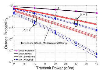
(a) OP for different turbulence conditions over light fog.

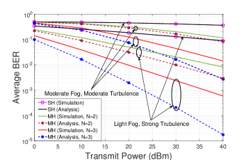
(b) ABER over different fog and turbulence conditions.

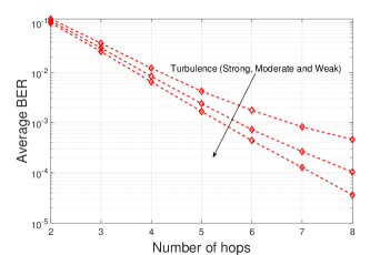
(c) ABER over light fog and different turbulence conditions at transmit power $P_{i}=10{\rm{dBm}}$.

Figure 2: Performance for long-range OWC systems over random fog, atmospheric turbulence with pointing error parameters $\frac{w_{z}}{a_{r}}=6$ and $\sigma_{s}=5~{}{\rm{cm}}$ .

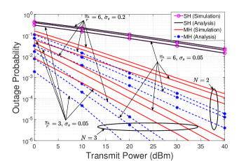
(a) OP analysis over light fog with different pointing errors conditions.

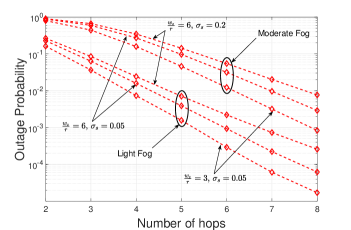
(b) OP analysis over light fog and moderate fog with different pointing errors conditions at transmit power $P_{i}=10{\rm{dBm}}$.

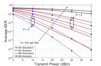
(c) ABER over moderate fog with pointing error parameters $\frac{w_{z}}{a_{r}}=6$ and $\sigma_{s}=5~{}{\rm{cm}}$.

Figure 3: Performance for short-range OWC systems over random fog and pointing errors.

V Simulation and Numerical Analysis

In this section, we investigate the performance of multihop OWC system over atmospheric turbulence and fog with generalized pointing errors using both numerical and Monte Carlo (MC) simulation (averaged over $10^{7}$ channel realizations) approaches. We use $20$ terms of the series expansion to numerically evaluate the derived expressions. We consider two simulation scenarios: short-range (link distance limited to $1000$ m) communication over fog with generalized pointing errors and long-range (link distance above $1000$ m) communication over atmospheric turbulence and fog with generalized pointing errors. We validate our derived analytical expressions with numerical and simulation results. We demonstrate the significance of multihop relaying as compared with the single-hop transmission for various link distances and channel impairments (turbulence, fog, and pointing errors). We list the simulation parameters in Table III.

In Fig. 2, we demonstrate the significance of multihop relaying for the OWC system under the combined effect of atmospheric turbulence, pointing errors, and random fog. We consider different atmospheric turbulence conditions (weak, moderate, and strong) with light fog and compare the OP with the single-hop, two hops, and three hops OWC system, as depicted in Fig. 2(a). The impact of turbulence intensity is not significant if the performance degradation with strong turbulence is compared with the weak one. Further, multihop relaying with $N=3$ significantly improves the OP.

We take two scenarios where the inverse correlation between turbulence and fog has been adopted by considering strong turbulence with light fog and moderate turbulence in the high-density moderate fog condition. We plot the ABER performance of the direct link, two hop, and three hop OWC system, as shown in Fig. 2(b). The ABER performance is extremely poor for both moderate and light foggy conditions with the direct transmission for the link distance of $1500$m. However, the ABER is significantly improved when the multihop relaying is employed. A dual-hop transmission is sufficient to achieve an acceptable ABER of $10^{-3}$ at a transmit power in light fog, where a few additional hops are required to achieve the same performance in moderate fog conditions. In Fig. 2(c), we describe the impact of the number of hops on the ABER performance for different turbulence conditions (weak, moderate, and strong). The figure shows the performance scaling with the number of hops achieving an acceptable ABER of $10^{-3}$ within $5$ hops at a $10$dBm transmit power.

In Fig. 3, we demonstrate the performance of OWC for short-range communication under the combined effect of random fog and pointing errors with negligible atmospheric turbulence. We plot the OP of the OWC system for short-range communication, as depicted in Fig. 3(a). We demonstrate the impact of fog density and pointing errors on the performance of multihop OWC system by considering a single hop (direct link), two hops, and three hops scenarios. It can be seen from Fig. 3(a) that there is a significant improvement in the OP performance with an increase in the number of hops. The figure shows that single hop transmission is not useful even at a transmit power of $40$dBm with OP more than $10^{-2}$. The dual-hop and triple-hop transmissions attain an acceptable OP in the range of $10^{-4}$ and $10^{-6}$, respectively. We can also observe the impact of pointing errors parameters ($\frac{w_{z}}{a_{r}}=\{3,6\}$ and $\sigma_{s}=\{5-20\}~{}{\rm{cm}}$) on the OP. In Fig. 3(b), we plot the OP versus the number of hops at a transmit power $10$dBm to show the scaling of performance considering light and moderate fog with different pointing errors parameters ($\frac{w_{z}}{a_{r}}=\{3,6\}$ and $\sigma_{s}=\{5-20\}~{}{\rm{cm}}$). The figure shows that the OP improves as we increase the number of hops. The number of hops required is less in the light foggy condition than the moderate fog to achieve an acceptable OP of $10^{-3}$.

In Fig. 3(c), we illustrate the ABER performance for short-range OWC system over the foggy channel with pointing errors. We demonstrate the effect of multihop relaying on the ABER performance for moderate foggy conditions and pointing errors ($\frac{w_{z}}{a_{r}}=6$ and $\sigma_{s}=5~{}{\rm{cm}}$) at two link distances ($\{d=0.8,1\}~{}{\rm{km}}$). The figure shows that the ABER is too high for practical practices in a single hop transmission for moderate fog conditions. However, the use of two relays (i.e., $N=3$ hops) significantly improves the ABER performance of the OWC system.

VI Conclusion

We analyzed the performance of a fixed-gain AF relaying based multihop OWC system over atmospheric turbulence and non-zero boresight pointing errors with fog-induced fading. We also analyzed a particular multihop system for short-range communication without considering atmospheric turbulence. We presented the OP and ABER performance for both multihop systems by deriving closed-form expressions for the PDF and CDF of the end-to-end SNR. We also developed performance metrics for the single-hop system to compare with the multihop transmission. The diversity order of the considered systems is presented using asymptotic analysis in high SNR to provide better insight into the performance dependency with various channel and system parameters. We presented extensive simulation results to demonstrate the significance of multihop relaying to extend the communication range. The single-hop transmission does not provide acceptable performance for a longer link over $1500$ m under foggy conditions. Further, there exists a gap between the derived upper bounds and simulation results when the number of hops increases. However, the OWC system requires a few hops only to achieve acceptable performance for a typical terrestrial communication advocating the significance of analytical bounds. A dual-hop transmission is sufficient to achieve an acceptable outage and error performance in light fog, where a few additional hops are required to achieve the same performance in moderate fog conditions.

We envision that the proposed multihop transmission considering generalized fading scenarios would be helpful to assess the deployment of the OWC system for terrestrial backhaul/fronthaul applications.

Appendix A: Lemma 1 (long-range and Single-Hop)

Applying the theory of product distribution, the PDF of $h_{{tp}_{i}}=h_{p_{i}}h_{t_{i}}$ can be expressed as

$$f_{h_{{tp}_{i}}}(x)=\int_{0}^{A_{i}}\frac{1}{|h_{p_{i}}|}f_{h_{t_{i}}}(x/h_{p_{i}})f_{h_{p_{i}}}(h_{p_{i}})dh_{p_{i}}$$ (100)

We use the identity $\frac{1}{(pt+1)^{q}}=G_{1,1}^{1,1}\left[\begin{matrix}1-q\\ 0\end{matrix}\bigg{|}pt\right]$ [[48], Eq. (8.4.2.5)] in (7), we express the PDF of $\cal{F}$ distribution $f_{h_{t_{i}}}(x)$ by

$$f_{h_{t_{i}}}(x)=\frac{a_{i}^{a_{i}}x^{a_{i}-1}}{\beta(a_{i},b_{i})(b_{i}-1)^{a_{i}}}G_{1,1}^{1,1}\left[\begin{matrix}1-(a_{i}+b_{i})\\ 0\end{matrix}\bigg{|}Bx\right]$$ (101)

Substituting (8) and (101) in (100), and applying the definition of Meijer’s G-function, we get

$$f_{h_{{tp}_{i}}}(x)=\frac{a_{i}^{a_{i}}\rho_{i}^{2}\exp\left(\frac{-s_{i}^{2}}{2\sigma_{i}^{2}}\right)x^{a_{i}-1}}{\beta(a_{i},b_{i})(b_{i}-1)^{a_{i}}A_{i}^{\rho_{i}^{2}}}\sum_{j=0}^{\infty}\frac{1}{(j!)^{2}}\left(\frac{s_{i}^{2}w^{2}_{z_{\rm{eq_{i}}}}}{8\sigma_{i}^{4}}\right)^{j}$$

$$\Big{(}\frac{1}{2\pi\jmath}\int_{\cal{L}}\Gamma(-u)\Gamma((a_{i}+b_{i})+u)\left(B_{i}x\right)^{u}du\Big{)}I_{1}$$ (102)

where $I_{1}=\int_{0}^{A_{i}}h^{\rho_{i}^{2}-a_{i}-u_{i}-1}_{p_{i}}\left(\ln\frac{A_{i}}{h_{p_{i}}}\right)^{j}dh_{p_{i}}$. Substituting $\log\frac{A_{i}}{h_{p_{i}}}=t$, we get $I_{1}=A^{\rho_{i}^{2}-a_{i}-u_{i}}_{i}\int_{0}^{\infty}e^{-(\rho_{i}^{2}-a_{i}-u_{i})t}t^{j}dt=A^{\rho_{i}^{2}-a_{i}-u_{i}}_{i}\frac{\Gamma(1+j)}{(\rho_{i}^{2}-a_{i}-u_{i})^{1+j}}=A^{\rho_{i}^{2}-a_{i}-u_{i}}_{i}\frac{\Gamma(1+j)[\Gamma(\rho_{i}^{2}-a_{i}-u_{i})]^{1+j}}{[\Gamma(1+\rho_{i}^{2}-a_{i}-u_{i})]^{1+j}}$. Thus, using $I_{1}$ in (102) and applying the definition of Meijer G-function, we get the combine PDF of $\cal{F}$-turbulence with the non-zero boresight pointing error

$$f_{h_{{tp}_{i}}}(x)=\frac{a_{i}^{a_{i}}\rho_{i}^{2}\exp\left(\frac{-s_{i}^{2}}{2\sigma_{i}^{2}}\right)}{A^{a_{i}}_{i}\beta(a_{i},b_{i})(b_{i}-1)^{a_{i}}}\sum_{j=0}^{\infty}\frac{1}{j!}\left(\frac{s_{i}^{2}w^{2}_{z_{\rm{eq_{i}}}}}{8\sigma_{i}^{4}}\right)^{j}$$

$$x^{a_{i}-1}G_{2+j,2+j}^{2+j,1}\left[\begin{array}[]{c}1-a_{i}-b_{i},\{1+\rho_{i}^{2}-a_{i}\}_{0}^{j+1}\\ 0,\{\rho_{i}^{2}-a_{i}\}_{0}^{j+1}\end{array}\left|\frac{Bx}{A_{i}}\right.\right]$$ (105)

Note that (105) generalizes the result presented in [28] for zero boresight model.

Similarly, we apply the product distribution of two random variables in $h_{i}=h_{{tp}_{i}}h_{f_{i}}$ to get the PDF of the combined channel $f_{h_{i}}(x)$. Using the transformation on $\gamma_{i}=\bar{\gamma}_{i}|h_{i}|^{2}$, we get the PDF of SNR for the combined channel in (LABEL:combine_pdf_fpt_series). We use (LABEL:combine_pdf_fpt_series) in $F^{\rm{LR}}_{\gamma_{i}}(\gamma)=\int_{0}^{\gamma}f^{\rm{LR}}_{\gamma_{i}}(\gamma)d\gamma$ to derive the CDF of SNR for the combined channel given in (16), which concludes the proof of Lemma 1.

Appendix B: Theorem 1 (long-range and Multihop)

First, we use (LABEL:combine_pdf_fpt_series) in (18) and substitute $\sqrt{\gamma}=t$ to get the $u$-th moment of SNR as:

$$\mathbb{E}[\gamma^{u}_{i}]=\frac{a_{i}^{a_{i}}z_{i}^{k_{i}}\rho_{i}^{2}\exp\left(\frac{-s_{i}^{2}}{2\sigma_{i}^{2}}\right)}{(A_{i}\sqrt{\bar{\gamma}_{i}})^{a_{i}}\beta(a_{i},b_{i})(b_{i}-1)^{a_{i}}}\sum_{j=0}^{\infty}\frac{1}{j!}\left(\frac{s_{i}^{2}w^{2}_{z_{\rm{eq_{i}}}}}{8\sigma_{i}^{4}}\right)^{j}$$

$$\int_{0}^{\infty}t^{2(u\frac{\phi_{i}}{N}+a_{i})-1}G_{2+j+k_{i},2+j+k_{i}}^{2+j+k_{i},1}$$

$$\Bigg{[}\begin{array}[]{c}1-a_{i}-b_{i},\{1+\rho_{i}^{2}-a_{i}\}_{0}^{j+1},\{1+z_{i}-a_{i}\}_{1}^{k_{i}}\\ 0,\{\rho_{i}^{2}-a_{i}\}_{0}^{j+1},\{z_{i}-a_{i}\}_{1}^{k_{i}}\end{array}$$ (108)

$$\left|\frac{B_{i}}{A_{i}\sqrt{\bar{\gamma}_{i}}}t\right.\Bigg{]}dt$$ (109)

Using the identity [49, eq. 07.34.21.0009.01] in (109), we get

$$\mathbb{E}[\gamma^{u}_{i}]=\frac{a_{i}^{a_{i}}z_{i}^{k_{i}}\rho_{i}^{2}\exp\left(\frac{-s_{i}^{2}}{2\sigma_{i}^{2}}\right)}{(A_{i}\sqrt{\bar{\gamma}_{i}})^{a_{i}}\beta(a_{i},b_{i})(b_{i}-1)^{a_{i}}}\sum_{j=0}^{\infty}\frac{1}{j!}\left(\frac{s_{i}^{2}w^{2}_{z_{\rm{eq_{i}}}}}{8\sigma_{i}^{4}}\right)^{j}$$

$$\frac{\big{[}\Gamma(a_{i}+\rho^{2}_{i}+2\frac{\phi_{i}}{N}u)\big{]}^{j+1}\big{[}\Gamma(a_{i}+z_{i}+2\frac{\phi_{i}}{N}u)\big{]}^{k_{i}}\Gamma(2a_{i}+2\frac{\phi_{i}}{N}u)}{\left[\Gamma\left(1+a_{i}+\rho^{2}_{i}+2\frac{\phi_{i}}{N}u\right)\right]^{j+1}\left[\Gamma\left(1+a_{i}+z_{i}+2\frac{\phi_{i}}{N}u\right)\right]^{k_{i}}}$$

$$\left(\frac{B_{i}}{A_{i}\sqrt{\bar{\gamma}_{i}}}\right)^{-2(u\frac{\phi_{i}}{N}+a_{i})}$$ (110)

Substituting (110) in (17), applying the definition of Fox’s H-function and using the transformation on $\gamma_{i}=\bar{\gamma}_{i}|h_{i}|^{2}$, we get the PDF of SNR for long-range multihop transmission in (22). Integrating the derived PDF $F^{\rm{LR}}_{\gamma_{i}}(\gamma)=\int_{0}^{\gamma}f^{\rm{LR}}_{\gamma_{i}}(\gamma)d\gamma$ with the standard mathematical procedure, we get the CDF of end-to-end SNR in (26).

Appendix C: Lemma 2 (short-range and Single-Hop)

Using the product distribution in $h_{{fp}_{i}}=h_{f_{i}}h_{p_{i}}$ for the joint PDF of the foggy channel and generalized pointing errors, we represent

$$f_{h_{{fp}_{i}}}(x)=\int_{h_{{fp}_{i}}/A_{i}}^{1}\frac{1}{|h_{f_{i}}|}f_{h_{p_{i}}}(x/h_{f_{i}})f_{h_{f_{i}}}(h_{f_{i}})dh_{f_{i}}$$ (111)

Substituting (5) and (8) in (111), we get

$$f_{h_{{fp}_{i}}}(x)=\frac{z_{i}^{k_{i}}\rho_{i}^{2}\exp\left(\frac{-s_{i}^{2}}{2\sigma_{i}^{2}}\right)}{\Gamma(k_{i})A_{i}^{\rho_{i}^{2}}}\sum_{j=0}^{\infty}\frac{1}{(j!)^{2}}\left(\frac{s_{i}^{2}w^{2}_{z_{\rm{eq_{i}}}}}{8\sigma_{i}^{4}}\right)^{j}x^{\rho_{i}^{2}-1}$$

$$\int_{h_{{fp}_{i}}/A_{i}}^{1}h^{m-1}_{f_{i}}\left(\log\frac{1}{h_{f_{i}}}\right)^{k_{i}-1}\left(\ln\frac{A_{i}h_{f_{i}}}{x}\right)^{j}dh_{f_{i}}$$ (112)

where $m_{i}=z_{i}-\rho_{i}^{2}$. Substituting $\log(1/h_{f_{i}})=t$ and using binomial expansion $(1-x)^{n}=\sum_{j=0}^{n}\left(\begin{array}[]{c}n\\ j\end{array}\right)(1)^{n-j}(-x)^{j}$ in (112), and using the definition incomplete Gamma function, we get

$$f_{h_{{fp}_{i}}}(x)=\frac{z_{i}^{k_{i}}\rho_{i}^{2}\exp\left(\frac{-s_{i}^{2}}{2\sigma_{i}^{2}}\right)}{\Gamma(k_{i})A_{i}^{\rho_{i}^{2}}}\sum_{j=0}^{\infty}\frac{1}{(j!)^{2}}\left(\frac{s_{i}^{2}w^{2}_{z_{\rm{eq_{i}}}}}{8\sigma_{i}^{4}}\right)^{j}$$

$$x^{\rho_{i}^{2}-1}\sum_{n=0}^{j}\left(\begin{array}[]{c}j\\ n\end{array}\right)(-1)^{n}\left(\ln\frac{A_{i}}{x}\right)^{j-n}{m_{i}}^{-n-k_{i}}$$ (115)

$$\left[\Gamma(n+k_{i})-\Gamma\left(n+k_{i},m_{i}\ln\frac{A_{i}}{x}\right)\right]$$ (116)

Using the transformation $\gamma_{i}=|h_{{fp}_{i}}|^{2}\bar{\gamma}_{i}$ in (116), we get the PDF of SNR for OWC system over the foggy channel with generalized pointing errors in (46). The CDF of SNR for foggy channel with generalized pointing errors can be obtained using (46) in $F^{\rm{SR}}_{\gamma_{i}}(\gamma)=\int_{0}^{\gamma}f^{\rm{SR}}_{\gamma_{i}}(\gamma)d\gamma$, which results into (50).

Appendix D: Theorem 2 (short-range and Multihop)

Using (46) in (18) and substituting $m_{i}\ln\frac{A_{i}\sqrt{\bar{\gamma}_{i}}}{\sqrt{\gamma}}=t$ and $d\gamma=-\frac{2}{m_{i}}A^{2}_{i}\bar{\gamma}_{i}\exp\left(-\frac{2}{m_{i}}t\right)dt$ and applying the series expansion of incomplete Gamma function $\Gamma(a,t)\triangleq(a-1)!e^{-t}\sum_{l=0}^{a-1}\frac{t^{l}}{l!}$[50], we get

$$\mathbb{E}[\gamma^{u}_{i}]=\frac{z_{i}^{k_{i}}\rho_{i}^{2}\exp\left(\frac{-s_{i}^{2}}{2\sigma_{i}^{2}}\right)}{m_{i}^{j+k_{i}+1}\Gamma(k_{i})}(A^{2}_{i}\bar{\gamma}_{i})^{u\frac{\phi_{i}}{N}}\sum_{j=0}^{\infty}\frac{1}{(j!)^{2}}\left(\frac{s_{i}^{2}w^{2}_{z_{\rm{eq_{i}}}}}{8\sigma_{i}^{4}}\right)^{j}$$

$$\sum_{n=0}^{j}\left(\begin{array}[]{c}j\\ n\end{array}\right)(-1)^{n}\Big{[}\Gamma(n+k_{i})\int_{0}^{\infty}t^{j-n}$$ (119)

$$\exp(-(2u\frac{\phi_{i}}{m_{i}N}+\frac{\rho^{2}_{i}}{m_{i}})t)dt-(n+k-1)!$$

$$\sum_{l=0}^{n+k-1}\frac{1}{l!}\int_{0}^{\infty}t^{j-n+l}\exp(-(2u\frac{\phi_{i}}{m_{i}N}+\frac{\rho^{2}_{i}}{m_{i}}+1)t)dt\Big{]}$$ (120)

To represent the $u$-th moment in terms of Gamma functions, we solve (120) using the identity $\int_{0}^{\infty}t^{a}\exp(-bt)dt=b^{-a-1}\Gamma(a+1)$ and $\frac{1}{u}=\frac{\Gamma(u)}{\Gamma(1+u)}$ as:

$$\mathbb{E}[\gamma^{u}_{i}]=\frac{z_{i}^{k_{i}}\rho_{i}^{2}\exp\left(\frac{-s_{i}^{2}}{2\sigma_{i}^{2}}\right)}{m_{i}^{j+k_{i}+1}\Gamma(k_{i})}(A^{2}_{i}\bar{\gamma}_{i})^{u\frac{\phi_{i}}{N}}\sum_{j=0}^{\infty}\frac{1}{(j!)^{2}}\left(\frac{s_{i}^{2}w^{2}_{z_{\rm{eq_{i}}}}}{8\sigma_{i}^{4}}\right)^{j}$$

$$\sum_{n=0}^{j}\left(\begin{array}[]{c}j\\ n\end{array}\right)(-1)^{n}\Big{[}\Gamma(n+k_{i})\Gamma(1+j-n)$$ (123)

$$\left(\frac{\Gamma\left(\frac{\rho_{i}^{2}}{m_{i}}+\frac{2\phi_{i}}{m_{i}N}u\right)}{\Gamma\left(1+\frac{\rho_{i}^{2}}{m_{i}}+\frac{2\phi_{i}}{m_{i}N}u\right)}\right)^{n-j-1}-(n+k-1)!$$

$$\sum_{l=0}^{n+k-1}\frac{1}{l!}\Gamma(1+j-n+l)\left(\frac{\Gamma\left(1+\frac{\rho_{i}^{2}}{m_{i}}+\frac{2\phi_{i}}{m_{i}N}u\right)}{\Gamma\left(2+\frac{\rho_{i}^{2}}{m_{i}}+\frac{2\phi_{i}}{m_{i}N}u\right)}\right)^{n-j-l-1}\Big{]}$$ (124)

Thus, invoking (124) in (17) and applying the definitions of Fox’s H-function, we get PDF of SNR for multihop transmission in (59). The CDF is driven by applying standard mathematical steps in $F^{\rm{SR}}_{\gamma_{i}}(\gamma)=\int_{0}^{\gamma}f^{\rm{SR}}_{\gamma_{i}}(\gamma)d\gamma$ to get (68), which concludes the proof of Theorem 2.

References

- [1] M. A. Khalighi and M. Uysal, “Survey on free space optical communication: A communication theory perspective,” IEEE Communications Surveys Tutorials, vol. 16, no. 4, pp. 2231–2258, 2014.
- [2] H. Kaushal and G. Kaddoum, “Optical communication in space: Challenges and mitigation techniques,” IEEE Communications Surveys Tutorials, vol. 19, no. 1, pp. 57–96, 2017.
- [3] M. Alzenad, M. Z. Shakir, H. Yanikomeroglu, and M.-S. Alouini, “FSO-based vertical backhaul/fronthaul framework for 5G+ wireless networks,” IEEE Communications Magazine, vol. 56, no. 1, pp. 218–224, 2018.
- [4] G. Xu and Z. Song, “Effects of solar scintillation on deep space communications: Challenges and prediction techniques,” IEEE Wireless Communications, vol. 26, no. 2, pp. 10–16, 2019.
- [5] M. Aggarwal, P. Garg, and P. Puri, “Dual-hop optical wireless relaying over turbulence channels with pointing error impairments,” Journal of Lightwave Technology, vol. 32, no. 9, pp. 1821–1828, 2014.
- [6] L. Yang, X. Gao, and M.-S. Alouini, “Performance analysis of relay-assisted all-optical FSO networks over strong atmospheric turbulence channels with pointing errors,” Journal of Lightwave Technology, vol. 32, no. 23, pp. 4613–4620, 2014.
- [7] J. Libich, M. Komanec, S. Zvanovec, P. Pesek, W. O. Popoola, and Z. Ghassemlooy, “Experimental verification of an all-optical dual-hop Gbit/s free-space optics link under turbulence regimes,” Opt. Lett., vol. 40, no. 3, pp. 391–394, Feb 2015.
- [8] E. Zedini, H. Soury, and M.-S. Alouini, “Dual-hop FSO transmission systems over Gamma–Gamma turbulence with pointing errors,” IEEE Transactions on Wireless Communications, vol. 16, no. 2, pp. 784–796, 2017.
- [9] T. A. Tsiftsis, H. G. Sandalidis, G. K. Karagiannidis, and N. C. Sagias, “Multihop free-space optical communications over strong turbulence channels,” in 2006 IEEE International Conference on Communications, vol. 6, 2006, pp. 2755–2759.
- [10] S. M. Aghajanzadeh and M. Uysal, “Multi-hop coherent free-space optical communications over atmospheric turbulence channels,” IEEE Transactions on Communications, vol. 59, no. 6, pp. 1657–1663, 2011.
- [11] M. Safari, M. M. Rad, and M. Uysal, “Multi-hop relaying over the atmospheric poisson channel: Outage analysis and optimization,” IEEE Transactions on Communications, vol. 60, no. 3, pp. 817–829, 2012.
- [12] M. A. Kashani and M. Uysal, “Outage performance and diversity gain analysis of free-space optical multi-hop parallel relaying,” Journal of Optical Communications and Networking, vol. 5, no. 8, pp. 901–909, 2013.
- [13] P. Wang, T. Cao, L. Guo, R. Wang, and Y. Yang, “Performance analysis of multihop parallel free-space optical systems over exponentiated weibull fading channels,” IEEE Photonics Journal, vol. 7, no. 1, pp. 1–17, 2015.
- [14] P. Wang, J. Zhang, L. Guo, T. Shang, T. Cao, R. Wang, and Y. Yang, “Performance analysis for relay-aided multihop BPPM FSO communication system over exponentiated weibull fading channels with pointing error impairments,” IEEE Photonics Journal, vol. 7, no. 4, pp. 1–20, 2015.
- [15] P. Wang, T. Cao, L. Guo, X. Liu, H. Fu, R. Wang, and Y. Yang, “Multihop FSO over exponentiated weibull fading channels with nonzero boresight pointing errors,” IEEE Photonics Technology Letters, vol. 28, no. 16, pp. 1747–1750, 2016.
- [16] C. Ben Issaid, K.-H. Park, and M.-S. Alouini, “A generic simulation approach for the fast and accurate estimation of the outage probability of single hop and multihop FSO links subject to generalized pointing errors,” IEEE Transactions on Wireless Communications, vol. 16, no. 10, pp. 6822–6837, 2017.
- [17] C. K. Datsikas, K. P. Peppas, N. C. Sagias, and G. S. Tombras, “Serial free-space optical relaying communications over Gamma-Gamma atmospheric turbulence channels,” Journal of Optical Communications and Networking, vol. 2, no. 8, pp. 576–586, 2010.
- [18] E. Zedini and M.-S. Alouini, “Multihop relaying over IM/DD FSO systems with pointing errors,” Journal of Lightwave Technology, vol. 33, no. 23, pp. 5007–5015, 2015.
- [19] ——, “On the performance of multihop heterodyne FSO systems with pointing errors,” IEEE Photonics Journal, vol. 7, no. 2, pp. 1–10, 2015.
- [20] X. Tang, Z. Wang, Z. Xu, and Z. Ghassemlooy, “Multihop free-space optical communications over turbulence channels with pointing errors using heterodyne detection,” Journal of Lightwave Technology, vol. 32, no. 15, pp. 2597–2604, 2014.
- [21] W. G. Alheadary, K.-H. Park, and M.-S. Alouini, “Performance analysis of multi-hop heterodyne FSO systems over malaga turbulent channels with pointing error using mixture gamma distribution,” in 2017 IEEE 85th Vehicular Technology Conference (VTC Spring), 2017, pp. 1–5.
- [22] ——, “BER analysis of multi-hop heterodyne FSO systems with fixed gain relays over general malaga turbulence channels,” in 2017 13th International Wireless Communications and Mobile Computing Conference (IWCMC), 2017, pp. 1172–1177.
- [23] W. Pang, W. Chen, Y. Song, G. Li, P. Wang, M. Duan, and S. Li, “Performance analysis for multi-hop FSO communication system over M distribution with pointing errors,” in 2021 19th International Conference on Optical Communications and Networks (ICOCN), 2021, pp. 1–3.
- [24] B. Ashrafzadeh, A. Zaimbashi, E. Soleirnani-Nasab, and M. Uysal, “On the performance of multi-hop free space optical cooperative systems,” in 2018 IEEE Global Communications Conference (GLOBECOM), 2018, pp. 1–6.
- [25] B. Ashrafzadeh, A. Zaimbashi, E. Soleimani-Nasab, and M. Uysal, “Unified performance analysis of multi-hop FSO systems over double generalized gamma turbulence channels with pointing errors,” IEEE Transactions on Wireless Communications, vol. 19, no. 11, pp. 7732–7746, 2020.
- [26] G. Karagiannidis, T. Tsiftsis, and R. Mallik, “Bounds for multihop relayed communications in nakagami-m fading,” IEEE Transactions on Communications, vol. 54, no. 1, pp. 18–22, 2006.
- [27] K. P. Peppas, G. C. Alexandropoulos, E. D. Xenos, and A. Maras, “The fischer–snedecor -distribution model for turbulence-induced fading in free-space optical systems,” Journal of Lightwave Technology, vol. 38, no. 6, pp. 1286–1295, 2020.
- [28] O. S. Badarneh, R. Derbas, F. S. Almehmadi, F. El Bouanani, and S. Muhaidat, “Performance analysis of FSO communications over F turbulence channels with pointing errors,” IEEE Communications Letters, vol. 25, no. 3, pp. 926–930, 2021.
- [29] O. S. Badarneh and R. Mesleh, “Diversity analysis of simultaneous mmWave and free-space-optical transmission over -distribution channel models,” Journal of Optical Communications and Networking, vol. 12, no. 11, pp. 324–334, 2020.
- [30] L. Han, Y. Wang, X. Liu, and B. Li, “Secrecy performance of FSO using HD and IM/DD detection technique over -distribution turbulence channel with pointing error,” IEEE Wireless Communications Letters, vol. 10, no. 10, pp. 2245–2248, 2021.
- [31] W. M. R. Shakir and M.-S. Alouini, “Secrecy performance analysis of parallel FSO/mm-wave system over unified fisher-snedecor channels,” IEEE Photonics Journal, vol. 14, no. 2, pp. 1–13, 2022.
- [32] J. Ding, X. Xie, L. Tan, J. Ma, and D. Kang, “Dual-hop RF/FSO systems over shadowed and fisher-snedecor fading channels with non-zero boresight pointing errors,” Journal of Lightwave Technology, vol. 40, no. 3, pp. 708–719, 2022.
- [33] M. Khan, M. Awan, E. Leitgeb, F. Nadeem, and I. Hussain, “Selecting a distribution function for optical attenuation in dense continental fog conditions,” in 2009 International Conference on Emerging Technologies, 2009, pp. 142–147.
- [34] M. A. Esmail, H. Fathallah, and M.-S. Alouini, “Outdoor FSO communications under fog: Attenuation modeling and performance evaluation,” IEEE Photonics Journal, vol. 8, no. 4, pp. 1–22, Aug 2016.
- [35] M. A. Esmail, H. Fathallah, and M. Alouini, “On the performance of optical wireless links over random foggy channels,” IEEE Access, vol. 5, pp. 2894–2903, 2017.
- [36] ——, “Outage probability analysis of FSO links over foggy channel,” IEEE Photonics Journal, vol. 9, no. 2, pp. 1–12, 2017.
- [37] Z. Rahman, S. M. Zafaruddin, and V. K. Chaubey, “Performance of opportunistic beam selection for OWC system under foggy channel with pointing error,” IEEE Communications Letters, vol. 24, no. 9, pp. 2029–2033, Sep. 2020.
- [38] Z. Rahman, T. N. Shah, S. M. Zafaruddin, and V. K. Chaubey, “Performance of dual-hop relaying for OWC system over foggy channel with pointing errors and atmospheric turbulence,” IEEE Transactions on Vehicular Technology, pp. 1–1, Early Access, Dec. 2021.
- [39] A. A. Farid and S. Hranilovic, “Outage capacity optimization for free-space optical links with pointing errors,” Journal of Lightwave Technology, vol. 25, no. 7, pp. 1702–1710, July 2007.
- [40] M. Hasna and M.-S. Alouini, “Outage probability of multihop transmission over nakagami fading channels,” IEEE Communications Letters, vol. 7, no. 5, pp. 216–218, 2003.
- [41] K.-J. Jung, S. S. Nam, M.-S. Alouini, and Y.-C. Ko, “Unified finite series approximation of FSO performance over strong turbulence combined with various pointing error conditions,” IEEE Transactions on Communications, vol. 68, no. 10, pp. 6413–6425, 2020.
- [42] V. K. Chapala and S. M. Zafaruddin, “Unified performance analysis of reconfigurable intelligent surface empowered free-space optical communications,” IEEE Transactions on Communications, pp. 1–1, 2021.
- [43] P. Bhardwaj and S. M. Zafaruddin, “On the performance of multihop THz wireless system over mixed channel fading with shadowing and antenna misalignment,” arXiv: 2110.15952, 2021, Submitted to IEEE Transactions on Communications.
- [44] A. Kilbas, Analytical methods and special functions, H-Transforms: Theory and Applications. New York, NY, USA: Taylor and Francis, 2004.
- [45] B. Ashrafzadeh, E. Soleimani-Nasab, M. Kamandar, and M. Uysal, “A framework on the performance analysis of dual-hop mixed FSO-RF cooperative systems,” IEEE Transactions on Communications, vol. 67, no. 7, pp. 4939–4954, 2019.
- [46] Z. Rahman, S. M. Zafaruddin, and V. K. Chaubey, “Performance of opportunistic receiver beam selection in multiaperture OWC systems over foggy channels,” IEEE Systems Journal, vol. 14, no. 3, pp. 4036–4046, 2020.
- [47] P. Mittal and K. Gupta, “An integral involving generalized function of two variables,” Proceedings of the Indian Academy of Sciences, vol. 75, no. 9, pp. 117–123, 1972.
- [48] A. P. Prudnikov, Integrals and series. vol.3, More special functions ; A.P. Prudnikov, Yu. A. Brychkov, O.I. Marichev ; translated from the Russian by G.G.Gould. Gordon and Breach, 1998.
- [49] Wolfram. (2001) The Wolfram functions site. Internet. [Online]. Available: http://functions.wolfram.com
- [50] D. Zwillinger, Table of integrals, series, and products. Elsevier, 2014.