Two-path interference in resonance-enhanced few-photon ionization of Li atoms

Abstract

We investigate the resonance-enhanced few-photon ionization of atomic lithium by linearly polarized light whose frequency is tuned near the $2s-2p$ transition. Considering the direction of light polarization orthogonal to the quantization axis, the process can be viewed as an atomic “double-slit experiment” where the 2$p$ states with magnetic quantum numbers $m_{\ell}=\pm 1$ act as the slits. In our experiment, we can virtually close one of the two slits by preparing lithium in one of the two circularly polarized $2p$ states before subjecting it to the ionizing radiation. This allows us to extract the interference term between the two pathways and obtain complex phase information on the final state. The experimental results show very good agreement with numerical solutions of the time-dependent Schrödinger equation. The validity of the two-slit model is also analyzed theoretically using a time-dependent perturbative approach.

I Introduction

Two-path interference is one of the most intriguing and intensely studied phenomena in physics. It was first demonstrated in 1801 for optical light by Thomas Young in his well-known double-slit experiment [1]. The historic importance of this experiment for the development of quantum theory is hard to overstate, because it reveals the wave nature of massive particles such as electrons [2, 3], atoms [4], and even large molecules [5], thereby supporting de Broglie’s hypothesis of wave-particle duality [6]. Until today, this phenomenon has not lost its appeal, and it has been observed in numerous systems. On one hand, it allows to extract phase information on wave functions, which is commonly not directly observable. On the other hand, it is exploited in many quantum-control schemes, because the manipulation of the relative amplitudes of the two pathways makes it possible to control the final state with high sensitivity. In atomic and molecular scattering processes, examples include well-known effects like Feshbach, shape, and Fano resonances (e.g. [7, 8, 9, 10]), or atomic-scale double-slits formed by diatomic molecules exhibiting interferences in differential ionization cross sections due to ion [11, 12, 13, 14], electron [15, 16], or photon impact [17, 18].

Multiphoton ionization processes of single atoms expose two- and multipath interferences in a particularly clean way, because of the well-defined energy and limited angular-momentum transfer in photon absorption reactions. A prominent example is RABBITT (Reconstruction of Attosecond Beating by Interference of Two-photon Transitions) spectroscopy [19, 20, 21, 22], which has become the standard tool to characterize extreme-ultraviolet (XUV) attosecond pulse trains and allows the study of attosecond atomic dynamics in the time domain. Two-color ionization schemes using (lower) harmonic radiation [23, 24, 25, 26] enable the coherent control of the reactions’ final state via two-path interferences. Recently, other schemes have been considered, where double-slit structures in so-called Kramers-Henneberger states emerge through the distortion of a bound state by an external field, once again resulting in interference patterns [27]. Two-path interference has not only been observed in laser pulses but also using two mutually incoherent (i.e., without relative phase lock) continuous-wave (cw) lasers in the two-photon ionization of rubidium atoms [28], where the photon energies are tuned to two different resonances.

In the present study, two-path interference occurs in the ground-state ionization of lithium exposed to single-color femtosecond laser pulses, which are linearly polarized in the $y$ direction. The laser spectrum has its center wavelength at 660 nm and partially overlaps with the $2s-2p$ resonance at 671 nm. For the quantization axis chosen as the $z$ direction, the absorption of a single photon results in the excitation to the 2$p$ state coherently populating the two magnetic sublevels with $m_{\ell}=+1$ and $-1$, respectively. These two eigenstates resemble the two “slits” in analogy to Young’s double-slit scheme (see Fig. 1). From these two excited levels, the atom is ionized without further resonance enhancement by the absorption of two more photons from the same laser pulse. The final result is a superposition of electronic $p$ and $f$ continuum waves.

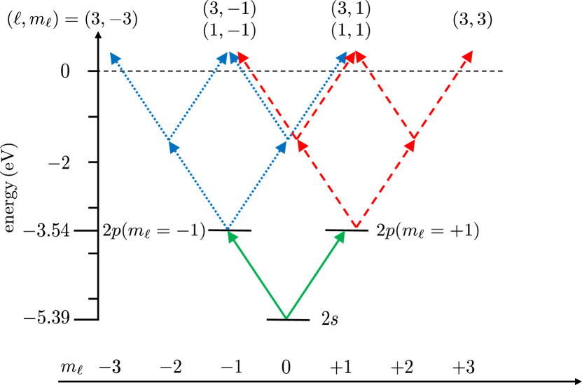
Figure 1: Few-photon ionization scheme in lowest-order perturbation theory. The ionization pathways from the 2$p$ state with $m_{\ell}=+1$ and $-1$ are shown as red dashed and blue dotted arrows, respectively. The 2$s$ ionization corresponds to the superposition of both.

It is important to note that the distinction of these two pathways relies on the choice of the quantization direction. However, this choice is motivated by the experimental capability of preparing the atoms selectively in one of the two excited and polarized magnetic sublevels of the 2$p$ state before exposing them to the femtosecond laser pulse. This enables us to measure not only the final intensity of the two interfering pathways, which corresponds to the differential cross sections for the ionization of the 2$s$ state, but also the intensity of each pathway individually via 2$p$ ionization. This fact can approximately be expressed as (see appendix A for a derivation and discussion of the validity criteria)

$$\left|\mathcal{A}_{2s}(\bm{p})\right|^{2}\approx\alpha\left|\mathcal{A}_{2p}^{+}(\bm{p})+\mathcal{A}_{2p}^{-}(\bm{p})\right|^{2},$$ (1)

where $\mathcal{A}_{2s}(\bm{p})$, $\mathcal{A}_{2p}^{+}(\bm{p})$, and $\mathcal{A}_{2p}^{-}(\bm{p})$ represent the ionization amplitudes for a photoelectron with asymptotic momentum $\bm{p}$ from the initial 2$s\,(m_{\ell}\!=\!0)$, 2$p\,(m_{\ell}\!=\!+1)$, and 2$p\,(m_{\ell}\!=\!-1)$ states, respectively, while $\alpha$ is a real factor. Equation (1) holds in our case under the assumptions that (i) the pulse is sufficiently long and the light frequency is tuned near the $2s-2p$ transition, such that only resonant transitions to the $2p$ states through the first photon absorption contribute (virtual excitations can be neglected), and (ii) the field is sufficiently weak that the ionization amplitude can be expressed through a perturbative expansion (even beyond the lowest order). While the transfer between $2s$ and $2p$ was adiabatic in our case, we found Eq. (1) to remain fairly accurate even for nonadiabatic transfer (see appendix A for more details). In addition, the experimental observations and calculations will be shown to be in excellent agreement, thereby providing further evidence of the validity of Eq. (1). Using this approach, we obtain a direct and intuitive way to extract the complex phase difference between $\mathcal{A}_{2p}^{+}$ and $\mathcal{A}_{2p}^{-}$ as a function of the electron emission angle, thereby revealing the effect of the orientation of the initial electron orbital angular momentum on the final state’s phase.

II Methods

The experimental technique and the theoretical method are identical to those reported in previous studies on very similar systems [29, 30, 31]. Therefore, only some key features are repeated here and parameters specific to the present study are mentioned.

Lithium atoms are cooled and confined in a volume of about 1 mm diameter in a near-resonant all-optical atom trap (AOT) [32] with a fraction of about 25 % being in the polarized excited $2p\,(m_{\ell}\!=\!+1)$ state and about 75 % in the 2$s$ ground state. The atoms are ionized in the field of a femtosecond laser based on a Ti:Sa oscillator with two noncollinear optical parametric amplifier (NOPA) stages. For the present study, the laser wavelength was chosen to center at 660 nm with pulse durations (FWHM of intensity) of about 65 fs and a peak intensity of about 3$\times$10¹⁰ W/cm². The three-dimensional electron momentum vectors are measured with a resolution of about 0.01 a.u. [33] in a reaction microscope, which is described in detail in [34, 35]. It is important to note that this experimental setup enables us to obtain differential cross-normalized data for the ionization of the 2$s$ and the 2$p$ initial states simultaneously.

In our theoretical model, the lithium atoms are approximated as a single active electron moving in the field of a 1$s^{2}$ ionic core. The latter is described by a static Hartree potential [36, 37], which is supplemented by phenomenological terms to account for the core polarizability as well as exchange between the valence electron and those in the core [29]. The (complex) final-state wave function is obtained after propagating the initial state in time by numerically solving the time-dependent Schrödinger equation (TDSE).

III Results and Discussion

In the present study, lithium atoms in the 2$s$ ground state and 2$p$ excited state are ionized in a laser field with a central wavelength of 660 nm at intensities well below 10¹¹ W/cm². This situation corresponds to Keldysh parameters $\gamma>20$, and hence the system is expected to be well described in a multiphoton picture. The two initial states are ionized by the absorption of (at least) three (from $2s$) or two (from $2p$) photons, respectively, resulting in a final electron energy of about 200 meV. The measured and calculated electron momentum spectra shown in Fig. 2 are in excellent agreement with each other. Before proceeding to the analysis of the two-path interference introduced above, two important features of the data should be mentioned, even though they were already reported previously in several recent studies [29, 31].

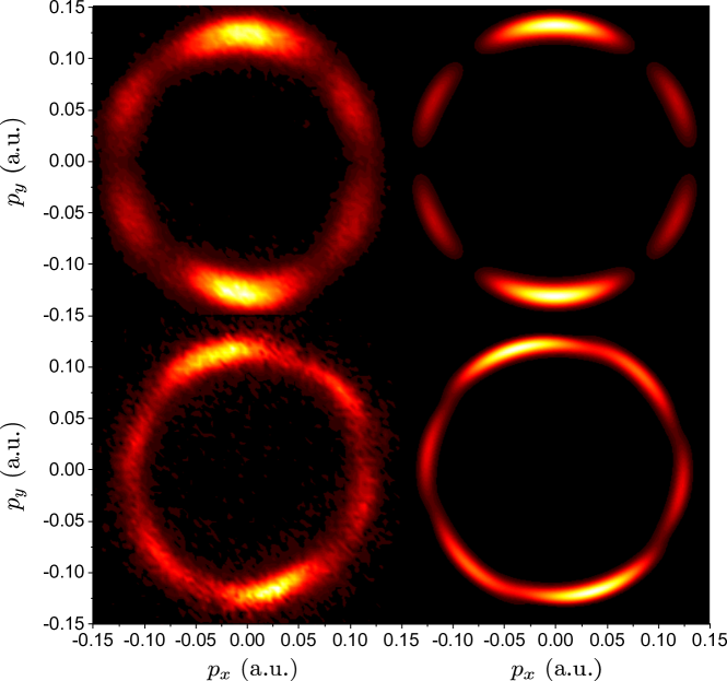
Figure 2: Experimental (left) and theoretical (right) photoelectron momentum distributions projected onto the $xy$ plane for few-photon ionization of the 2$s$ (top row) and 2$p\,(m_{\ell}\!=\!+1)$ (bottom row) initial states by linearly polarized laser pulses of 65 fs duration with a center wavelength of 660 nm and a peak intensity of 3.1$\times 10^{10}$ W/cm². The laser polarization direction is along the $y$ axis (i.e., vertical), while the atomic initial orbital angular momentum is oriented in the $z$ direction (i.e., perpendicular to the drawing plane).

First, while the photoelectron momentum distributions (PMDs) for 2$s$ ionization exhibit reflection symmetry with respect to the laser electric field direction (the vertical direction in the momentum spectra shown in Fig. 2), this symmetry is broken for ionization of the polarized 2$p$ state. Consequently, the main electron emission direction appears to be shifted. The dependence of this phenomenon, known as magnetic dichroism, on the laser wavelength and intensity was recently investigated by Acharya et al. [31]. In this earlier study, these asymmetries were explained in a partial-wave picture. They were traced back to a nonvanishing mean orientation of the final electron orbital angular momentum $\left<m_{\ell}\right>\neq 0$. This “remnant” of the initial target polarization is partially preserved throughout the ionization process. The angular shifts and observed asymmetries are a result of the interference between (phase-shifted) partial waves with different $m_{\ell}$.

Second, the azimuthal photoelectron angular distributions (PADs) for 2$p$ ionization feature six peaks. As discussed below, this indicates beyond lowest-order contributions to the ionization cross section. Generally, the dependence of the differential cross section on the azimuthal angle $\varphi$ is given by [31]

$$\frac{\mathrm{d}\sigma}{\mathrm{d}\Omega}=\left|\sum_{m_{\ell}}c_{m_{\ell}}e^{im_{\ell}\varphi}\right|^{2},$$ (2)

where the factors $c_{m_{\ell}}$ relate to the complex amplitudes of the partial waves. In lowest-order perturbation theory (LOPT), only the shortest pathways to the final state (i.e., the absorption of only the minimum number of photons needed to reach the final photoelectron energy) are considered. For the present initial 2$p\,(m_{\ell}\!=\!+1)$ state, this corresponds to two-photon absorption. In the electric dipole approximation, this results in partial waves with $m_{\ell}=-1$, $+1$, and $+3$ contributing to the final state (cf. Fig. 1). For this set of dipole-allowed $m_{\ell}$ values, therefore, the above expression results in a photoelectron angular distribution with no more than four peaks, in contrast to the six peaks observed in both the experiment and the ab initio calculation. This evident violation of LOPT close to the $2s-2p$ resonance was reported and discussed in our previous study as well: It is explained by the coupling between the 2$s$ and 2$p$ states in the external field giving rise to adiabatic population transfer between these two states and resulting in a contribution of $m_{\ell}=-3$ to the final state. Accounting for this additional pathway, the expression in Eq. (2) allows for angular distributions with up to six peaks, which is consistent with experiment and calculation.

The validity of the two-path interference expression given in Eq. (1) can be tested by using our theoretical description. In a first step, the $\mathcal{A}_{2p}^{-}$ and $\mathcal{A}_{2p}^{+}$ amplitudes for the ionization of the 2$p$ initial states with $m_{\ell}=-1$ and $+1$, respectively, are calculated. Their absolute squares, corresponding to the differential ionization cross sections, are shown as a function of the photoelectron momentum in Fig. 3 (left) considering only electron emission in the $xy$ plane (i.e., for a polar angle $\vartheta=90^{\circ}$). Due to symmetry considerations, the systems with opposite initial orbital angular momentum $m_{\ell}\!=\!+1$ and $-1$ are mirror images of one another with the mirror plane spanned by the laser polarization direction (the $y$ axis) and the direction of the initial atomic polarization (the $z$ axis). Specifically, $\mathcal{A}_{2p}^{+}(\sigma_{yz}\bm{p})=\mathcal{A}_{2p}^{-}(\bm{p})$, where $\sigma_{yz}$ is the reflection operator through the $yz$ plane.

In the second step, Eq. (1) is tested by comparing the calculated momentum distribution for 2$s$ ionization (corresponding to $\left|\mathcal{A}_{2s}\right|^{2}$) with the intensity of the superposition of the two amplitudes for 2$p$ ionization $\left|\mathcal{A}_{2p}^{+}+\mathcal{A}_{2p}^{-}\right|^{2}$. The PMDs obtained by both methods are shown in Fig. 3 (right and center, respectively). They are in overall very good agreement indeed, although the $\left|\mathcal{A}_{2s}\right|^{2}$ distribution has a slightly larger diameter. This small discrepancy is a result of slightly different (by approximately 10 %) photoelectron energies for 2$s$ and 2$p$ ionization, because the wavelength of the ionizing field is off the $2s-2p$ resonance by about 10 nm.

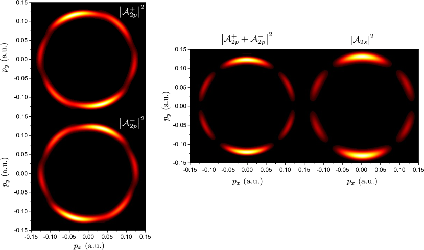
Figure 3: Absolute square of the calculated wave functions $\mathcal{A}_{2p}^{+}$ and $\mathcal{A}_{2p}^{-}$ (left), of their coherent sum $\mathcal{A}_{2p}^{+}+\mathcal{A}_{2p}^{-}$ (center), and of $\mathcal{A}_{2s}$ (right) in the $xy$ plane in momentum space. See text for details.

The discussion above shows that the final momentum distribution for 2$s$ ionization (which corresponds to $\left|\mathcal{A}_{2s}\right|^{2}$) can be calculated, to a good approximation, from the $\mathcal{A}_{2p}^{+}$ ionization amplitude by exploiting Eq. (1) and the mirror symmetry between $\mathcal{A}_{2p}^{+}$ and $\mathcal{A}_{2p}^{-}$. Evidently, this is not possible with the experimental data, because only the absolute square of the final-state wave function $|\mathcal{A}_{2p}^{+}|^{2}$ is directly measured. However, the relative phase between $\mathcal{A}_{2p}^{-}$ and $\mathcal{A}_{2p}^{+}$ can be extracted from Eq. (1) by reversing the above procedure and solving for the phase difference. This yields

$$\cos\Delta\phi(\bm{p})=\frac{\left|\mathcal{A}_{2s}(\bm{p})\right|^{2}-\alpha\left|\mathcal{A}_{2p}^{+}(\bm{p})\right|^{2}-\alpha\left|\mathcal{A}_{2p}^{-}(\bm{p})\right|^{2}}{2\alpha\left|\mathcal{A}_{2p}^{+}(\bm{p})\right|\left|\mathcal{A}_{2p}^{-}(\bm{p})\right|},$$ (3)

where $\Delta\phi(\bm{p})=\arg[\mathcal{A}_{2p}^{+*}(\bm{p})\mathcal{A}_{2p}^{-}(\bm{p})]$. The reconstruction of the phase difference $\Delta\phi$ in three-dimensional momentum space from experimental data using Eq. (3) requires matching photoelectron energies for 2$s$ and 2$p$ ionization, which is not strictly fulfilled for the present laser wavelength. The question arises whether, in spite of the small photoelectron energy mismatch, Eq. (3) is still applicable if only the dependence on the electron emission angle is considered (i.e., for the electron energy fixed at the peak energy). This can be the case, if the angular distributions do not significantly vary with small shifts of the photoelectron energy. This is tested by comparing the calculated angular distributions for 2$s$ ionization (extracted from $\left|\mathcal{A}_{2s}\right|^{2}$) with the distribution obtained for the interfering wave functions $\left|\mathcal{A}_{2p}^{+}+\mathcal{A}_{2p}^{-}\right|^{2}$.

The corresponding angular distributions are shown in Fig. 4. Indeed, the angular spectrum obtained from the interfering wave functions closely resembles the distribution calculated for 2$s$ ionization. There is only a small deviation in the relative intensity of the main peak in the polarization direction and the side peaks. Therefore, we conclude that Eq. (3) makes it possible to extract the phase difference $\Delta\phi$ (to a good approximation) as a function of the azimuthal angle for the peak photoelectron energy.

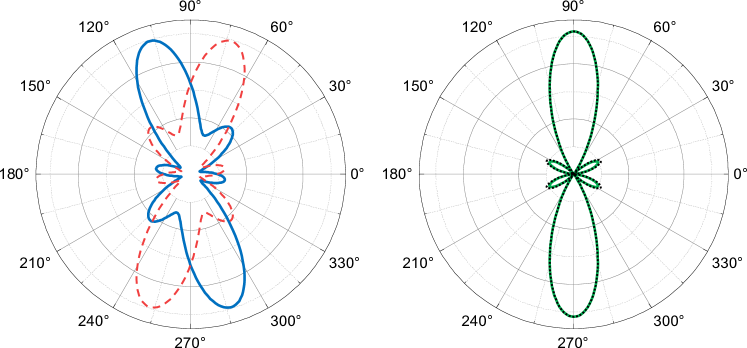
Figure 4: Angular distributions extracted from the wave functions in Fig. 3 as a function of the photelectron azimuthal angle $\varphi$. Left: angular distribution of $\left|\mathcal{A}_{2p}^{+}\right|^{2}$ (solid blue line) and $\left|\mathcal{A}_{2p}^{-}\right|^{2}$ (dashed red line). Right: $\left|\mathcal{A}_{2p}^{+}+\mathcal{A}_{2p}^{-}\right|^{2}$ (dashed black) and $\left|\mathcal{A}_{2s}\right|^{2}$ (solid green).

Before Eq. (3) can be employed to calculate the phase difference $\Delta\phi$ from the experimental data, the factor $\alpha$ must be determined. Here we can borrow an idea from Young’s double-slit experiment, where we know that the total flux is conserved, i.e., the total intensity equals the sum of the intensities going through each slit individually. In our case, this means that the momentum-integrated interference term in Eq. (1) should vanish, i.e.,

$$\int\mathrm{d}^{3}p\left|\mathcal{A}_{2p}^{+}(\bm{p})\right|\left|\mathcal{A}_{2p}^{-}(\bm{p})\right|\cos[\Delta\phi(\bm{p})]=0.$$ (4)

Equation (4) holds since the azimuthal dependence of the interference is expressed as the superposition of terms of the form $|c_{n}||c_{m}|\cos{[(n-m)\phi}]$, where $n\neq m$, and hence $\int_{0}^{2\pi}d\phi\cos{[(n-m)\phi]}=0$. Therefore, the interference term does not contribute to the total intensity, and the factor $\alpha$ is readily found as

$$\alpha=\frac{\int\mathrm{d}^{3}p\left|\mathcal{A}_{2p}^{+}(\bm{p})\right|^{2}+\int\mathrm{d}^{3}p\left|\mathcal{A}_{2p}^{-}(\bm{p})\right|^{2}}{\int\mathrm{d}^{3}p\left|\mathcal{A}_{2s}(\bm{p})\right|^{2}}.$$ (5)

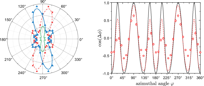
Figure 5: Left: Experimental PADs as a function of the azimuthal angle $\varphi$ for the few-photon ionization of lithium initially in the 2$s$ (solid green line) and 2$p$ state with $m_{\ell}\!=\!+1$ (blue solid line and open triangles) and $-1$ (red dashed line and solid squares). The lines are interpolating splines to guide the eye. Right: Experimental (red open circles) and theoretical (solid line) cosine of the phase difference as a function of the photoelectron azimuthal angle $\varphi$. The dashed red line is derived from the theoretical angular distributions that were convolved with the experimental resolution (see text).

The experimental PADs are shown in Fig. 5 (left). While the distributions for the ionization for the 2$s$ and the 2$p\,(m_{\ell}\!=\!+1)$ initial states are measured directly in our experiment, the data for 2$p\,(m_{\ell}\!=\!-1)$ are obtained by reflecting the data for the opposite target polarization on the laser polarization axis. Using these angular distributions, the cosine of the phase difference is calculated with Eq. (3), plotted in Fig. 5 (right), and compared to the theoretical predictions.

The distribution features six crests and troughs whose positions agree very well between theory and experiment. However, some discrepancies in the magnitude persist. While the calculated curve reaches the maximum and minimum values of +1 and $-1$, respectively, the oscillation is weaker in the experimental data. Generally, a value of $+1$ for $\cos\Delta\phi$ corresponds to maximum constructive interference, which is expected at angles where the angular distribution for 2$s$ ionization has a local maximum. Correspondingly, $\cos\Delta\phi=-1$ means complete destructive interference, which should occur at local minima in the differential 2$s$ ionization data.

There are two effects that might blur these interferences in the experimental data: (1) There is a small, but nonnegligible experimental angular uncertainty. The influence of this effect is shown by the red dashed line in the figure, which represents the $\cos\Delta\phi$ distribution derived from the theoretical angular distributions convolved with the experimental angular resolution (ca. 12^∘ FWHM). (2) The experimental data represent an average over a laser intensity range, as already discussed above. As the angular distributions are not entirely independent of the laser intensity (see Fig. 2), this will also result in a blurring of the data.

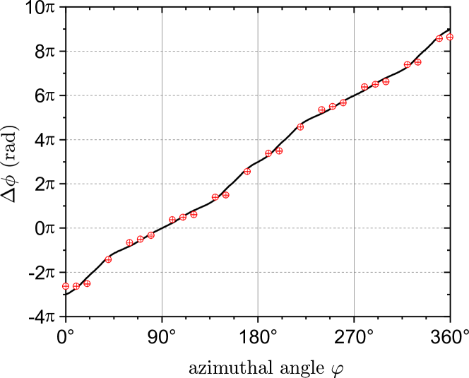
Figure 6: Theoretical (line) and experimental (open circles) phase difference of the final state wave functions after two-photon ionization of the 2$p$ initial state with $m_{\ell}=+1$ and $-1$ as a function of the photoelectron azimuthal angle.

The $\varphi$-dependence of the phase difference $\Delta\phi$ of the final-state wave functions can be derived from the data shown in Fig. 5 (right) and is presented in Fig. 6. It should be noted that extracting this phase difference is somewhat ambiguous due to the oscillatory behavior of the cosine function. In the present case we made the additional assumption that the phase increases monotonically with the azimuthal angle $\varphi$. The phase difference is $\Delta\phi=0$ at an angle of 90^∘ (i.e., in the $y$ direction) due to the symmetry $\Delta\phi(90+\varphi)=-\Delta\phi(90-\varphi)$. Overall, the phases obtained from the experimental data are consistent and in very good agreement with the theoretical prediction, thereby supporting the validity of the two-path interference picture developed here. The remaining deviations are attributed to the blurring effects discussed in the previous paragraph. It is important to note that the method used above does not allow to unambiguously extract the individual phases of the $\mathcal{A}_{2p}^{+}$ and $\mathcal{A}_{2p}^{-}$ amplitudes without using further assumptions, for example, when the angular dependence of the wave functions is expressed as a superposition of a limited set of spherical harmonics, as was done in Eq. (2).

IV Conclusions and Outlook

We studied the details of electron emission in few-photon ionization of lithium atoms initially either in the 2$s$ ground state or in the polarized 2$p\,(m_{\ell}\!=\!+1)$ excited state by radiation close to the $2s-2p$ resonance. We exploited the fact that the $2s$ state can be ionized through two possible pathways, specifically via the 2$p$ resonance with either $m_{\ell}\!=\!+1$ or $-1$. These two pathways interfere in the final state and resemble a double-slit. Because our experiment allows us to obtain the differential cross sections for the 2$s$ and the 2$p$ initial states separately, we are able to measure the final wave with both “slits” open, or with one “slit” closed. Therefore, the data make it possible to extract the interference term, thereby providing information on the relative phase of the two pathways. The experimentally obtained phase differences are in good agreement with our theoretical predictions.

Moreover, several interesting features are observed in the present data, which were reported for similar systems in preceding studies: First, the photoelectron angular distributions after ionization of the polarized 2$p$ state are not symmetric with respect to the laser polarization. Instead, the peaks are shifted. The wavelength and intensity dependence of this effect, known as magnetic dichroism, was systematically studied in [31]. Second, the peak structures in the present angle-differential spectra are in direct contradiction to the predictions of lowest-order perturbation theory, which is not applicable in resonant condition.

It is worth noting that the present method is not the only way to access information regarding the final state’s phase. Among the many possible approaches, a straightforward one is to fit the angular distributions with model functions described by a superposition of partial waves as expressed in Eq. (2). In some cases, this makes it possible to extract the relative phases between the complex amplitudes of partial waves contributing to the final state. For single-photon ionization, such complete studies were pioneered in the 1990s using polarized atomic targets [38, 39, 40]. In the multiphoton ionization regime, phase information was obtained by ionizing atoms with elliptically polarized light [41, 42] in a very similar way. In contrast, the present scheme, which exploits the resonance enhancement through two magnetic sublevels, provides direct, complete, and intuitive access to the interference term and the final-state phase.

Two- or multipath interferences in few-photon ionization are well suited for quantum control schemes, if the relative phases and intensities of the different paths can be regulated (e.g., [26]). It is interesting to conceive such a scheme for the present system. In fact, controlling the relative (complex) amplitudes of the transient 2$p\,(m_{\ell}\!=\!-1)$ and 2$p\,(m_{\ell}\!=\!+1)$ populations is experimentally straightforward. The transitions from the 2$s$ ground state to the two polarized excited 2$p$ levels are driven by left- and right-handed circularly polarized laser radiation, respectively, propagating in the $z$ direction. The superposition of these two fields with equal intensity and fixed relative phase corresponds to the linearly polarized light used in the present experiment. Changing the relative phase corresponds to a rotation of the polarization direction in the $xy$ plane.

Furthermore, a change in the relative intensities can be achieved by introducing an ellipticity to the radiation. In the present scheme, quasi-monochromatic light is used and changes of the laser polarization would also affect the ionization steps after populating the resonant 2$p$ levels. However, the effect on the excitation process and the ultimate ionization could be decoupled by using bichromatic laser fields with a weak contribution close to the $2s-2p$ resonance and a stronger contribution off resonance. Such an experiment would allow to prepare an atomic target in a coherent superposition of excited magnetic sublevels before ionizing it, thereby providing numerous possibilities to analyze and control the final state.

Appendix A Derivation and conditions of applicability of the two-pathway formula

We now derive Eq. (1) and discuss its domain of applicability. We consider the three-photon ionization amplitude $\mathcal{A}^{(3)}_{2s}(\bm{p})$ for the system initially in the Li $|2s\rangle$ ground state undergoing a transition to a photoelectron with asymptotic momentum $\bm{p}$. In the interaction picture, the amplitude is given by

$$\mathcal{A}^{(3)}_{2s}(\bm{p}) = \left(-\frac{i}{\hbar}\right)^{3}\sum_{i,j}\int_{t_{0}}^{\infty}dt_{1}\int_{t_{0}}^{t_{1}}dt_{2}\int_{t_{0}}^{t_{2}}dt_{3}$$

$$\times e^{i\frac{E}{\hbar}t_{1}}\hat{V}_{\bm{k},j}(t_{1})e^{-i\frac{E_{j}}{\hbar}(t_{1}-t_{2})}\hat{V}_{j,i}(t_{2})$$

$$\times e^{-i\frac{E_{i}}{\hbar}(t_{2}-t_{3})}\hat{V}_{i,2s}(t_{3})e^{-i\frac{E_{2s}}{\hbar}(t_{3}-t_{0})}.$$ (6)

In (6), $E_{i}$ are intermediate Li energies, $E_{2s}$ is the ground-state energy, $E={\hbar^{2}\bm{k}^{2}}/2m_{e}$ is the photoelectron energy, and $m_{e}$ is the electron mass. The summation runs over all bound and continuum electronic states. The elements $\hat{V}_{i,j}(t)=\langle i|\hat{V}(t)|j\rangle$ represent the time-dependent field-atom interaction between two electronic states $|i\rangle$ and $|j\rangle$, $\hat{V}(t)=e\bm{p}\cdot{\bm{A}}(t)$ is the dipole operator in the velocity gauge, ${\bm{A}}(t)=F(t)\sin(\omega t)\,\hat{\bm{e}}_{y}$ is the vector potential, and $F(t)$ is a smooth envelope that peaks at the maximum field strength.

Because the laser is tuned near the $2s\to 2p$ transition, we can restrict the first transition to the $|2p,m=\pm 1\rangle$ states. As a result, the amplitudes can be split into two terms

$$\mathcal{A}^{(3)}_{2s}(\bm{p}) = \mathcal{A}^{(3),+}_{2s}(\bm{p})+\mathcal{A}^{(3),-}_{2s}(\bm{p}),$$ (7)

where $\mathcal{A}^{(3),\pm}_{2s}(\bm{p})$ are the three-photon amplitudes with the first transition to one of the $|2p,m=\pm 1\rangle$ states. These amplitudes take the form

$$\mathcal{A}^{(3),\pm}_{2s}(\bm{p}) = e^{+i\frac{E_{2s}}{\hbar}t_{0}}\left(-\frac{i}{\hbar}\right)^{2}\sum_{j}\int_{t_{0}}^{\infty}dt_{1}\int_{t_{0}}^{t_{1}}dt_{2}e^{i\frac{E-E_{j}}{\hbar}t_{1}}$$ (8)

$$\times \hat{V}_{\bm{k},j}(t_{1})e^{i\frac{E_{j}-E_{2p}}{\hbar}t_{2}}\hat{V}_{j,2p\pm}(t_{2})a^{(1),\pm}_{2s\to 2p}(t_{2}),$$

where $\hat{V}_{j,2p\pm}(t_{2})=\langle j|\hat{V}(t_{2})|2p,m=\pm 1\rangle$ and $E_{2p}$ is the $2p$ state energy. In (7), we introduced the one-photon time-dependent transition amplitudes to the $2p$ states

$$a^{(1),\pm}_{2s\to 2p}(t_{2})=-\frac{i}{\hbar}\int_{t_{0}}^{t_{2}}dt_{3}\hat{V}_{2p\pm,2s}(t_{3})e^{i\frac{E_{2p}-E_{2s}}{\hbar}t_{3}}.$$ (9)

For light polarized along the $y$ axis, $a^{(1),+}_{2s\to 2p}=a^{(1),-}_{2s\to 2p}$.

We define the dynamical phase, $\Delta\phi(t)$, by

$$a^{(1),\pm}_{2s\to 2p}(t)=|a^{(1),\pm}_{2s\to 2p}(t)|e^{i[\phi_{0}+\Delta\phi(t)]}.$$ (10)

Because the detuning, $\Delta\omega=\omega-(E_{2p}-E_{2s})/\hbar$ is very small in our near-resonance condition ($\Delta\omega=30$ meV), the dynamical phase, $\Delta\phi(t)\approx(\Delta\omega)t$ varies very slowly. For weak fields, when interactions with other states are neglected (two-state model), the dynamical phase is identically zero in the resonance limit of $\Delta\omega=0$.

It is now possible to incorporate $a^{(1),\pm}_{2p\to 2p}(t_{2})$ in $\hat{V}(t_{2})$ and factor out the time-independent phase $\phi_{0}$. This leads to

$$\mathcal{A}^{(3),\pm}_{2s}(\bm{p}) = e^{i\beta}\left(-\frac{i}{\hbar}\right)^{2}\sum_{j}\int_{t_{0}}^{\infty}dt_{1}\int_{t_{0}}^{t_{1}}dt_{2}e^{i\frac{E}{\hbar}t_{1}}V_{\bm{k},j}(t_{1})$$ (11)

$$\times e^{-i\frac{E_{j}}{\hbar}(t_{1}-t_{2})}\bar{V}_{j,2p,\pm}(t_{2})e^{-i\frac{E_{2p}}{\hbar}t_{2}},$$

where $\beta=E_{2s}t_{0}/\hbar+\phi_{0}$ and $\bar{V}(t_{2})=a^{(1),\pm}_{2s\to 2p}(t_{2})\hat{V}(t_{2})$. This is the equivalent of introducing a new complex field, ${\bar{\bm{A}}}(t)=\bar{F}(t)\exp[{i\Delta\omega t}]\sin\omega t\;\hat{\bm{e}}_{y}$, for the second photon transition. Therefore, the new field has a frequency shifted by the detuning, $\pm\Delta\omega$, for emission/absorption, respectively, and a new envelope given by

$$\bar{F}(t)=F(t)|a^{(1),\pm}_{2s\to 2p}(t)|.$$ (12)

Because $|\Delta\omega|\ll\omega$ in our near-resonance condition, the frequency shift $\Delta\omega$ has a negligible effect on the second transition. In addition, for an adiabatic process as in our study, $|a^{(1),\pm}_{2s\to 2p}(t)|\propto F(t)$. Consequently, $\bar{F}(t)\propto F^{2}(t)$, which corresponds to an effective decrease of the pulse intensity and a reduction by two of the FWHM for a gaussian envelope. The broadening of the spectral width for a relatively long pulse also has a negligible impact on the final phase amplitude.

Therefore, the amplitude is simply rescaled when compared to photoionization directly from the $2p$ states with the field ${\bm{A}}(t)$, and we can write

$$\mathcal{A}^{(3),\pm}_{2s}(\bm{p})\approx\mathcal{A}_{2s\to 2p}\mathcal{A}^{(2),\pm}_{2p}(\bm{p}),$$ (13)

where $\mathcal{A}_{2s\to 2p}$ is a momentum-independent complex amplitude. The two-photon ionization amplitudes, starting from $|2p,m=\pm 1\rangle$, then take the form

$$\mathcal{A}_{2p}^{(2),\pm} = \left(-\frac{i}{\hbar}\right)^{2}\sum_{j}\int_{t_{0}}^{\infty}dt_{1}\int_{t_{0}}^{t_{1}}dt_{2}e^{i\frac{E}{\hbar}t_{1}}V_{\bm{k},j}(t_{1})$$ (14)

$$\times e^{-i\frac{E_{j}}{\hbar}(t_{1}-t_{2})}V_{j,2p,\pm}(t_{2})e^{-i\frac{E_{2p}}{\hbar}t_{2}}.$$

As a result, we obtain

$$|\mathcal{A}^{(3)}_{2s}(\bm{p})|^{2}\approx|\mathcal{A}_{2s\to 2p}|^{2}|\mathcal{A}_{2p}^{(2),+}(\bm{p})+\mathcal{A}_{2p}^{(2),-}(\bm{p})|^{2}.$$

In our case, higher-order processes might play a role even in the weak-field regime due to the near-resonance condition. However, the above reasoning applies in exactly the same way for higher-order processes. We generally obtain for the $(2n+1)$-photon amplitude

$$\mathcal{A}^{(2n+1),\pm}_{2s}(\bm{p})\approx\mathcal{A}_{2s\to 2p}\mathcal{A}^{(2n),\pm}_{2p}(\bm{p}).$$ (16)

Finally, summing up the different order terms and introducing $\alpha=|\mathcal{A}_{2s\to 2p}|^{2}$, which only depends on the $2s\to 2p$ transition, we obtain Eq. (1), i.e.

$$|\mathcal{A}_{2s}(\bm{p})|^{2}\approx\alpha|\mathcal{A}^{+}_{2p}(\bm{p})+\mathcal{A}^{-}_{2p}(\bm{p})|^{2}.$$ (17)

Numerically, we found the above relation to be quite robust against increasing the pulse intensity and, in particular, at intensities when the population transfer becomes nonadiabatic. This is explained by the fact that $\Delta\phi(t)\approx(\Delta\omega)t$ holds at higher intensities if one assumes negligible interactions with other states. Surprisingly, as Rabi oscillations become visible at slightly higher intensity ($\approx 10^{12}\,$W/cm²), Eq. (1) still remains relatively accurate. This is likely due to the fact that higher-order terms are able to describe population transfer between the $2s$ and $2p$ states. As Rabi oscillations take place, the effective envelope $\bar{F}(t)$ oscillates at the Rabi frequency $\Omega$, such that the pulse obtains two additional frequency components $\omega\pm\Omega$. This represents an alternative interpretation of the Autler-Towns splitting besides the dressed-state picture.

When the intensity keeps increasing, the perturbative expansion will break down and other states, besides $2p$, will start contributing to the first transition step. As a result, the approximation (7) will ultimately become inaccurate.

References

- Young [1802] T. Young, Philosophical Transactions of the Royal Society of London 92, 12 (1802).
- Davisson and Germer [1928] C. J. Davisson and L. H. Germer, Proceedings of the National Academy of Sciences 14, 317 (1928).
- Jönsson [1961] C. Jönsson, Zeitschrift für Physik 161, 454 (1961).
- Keith et al. [1991] D. W. Keith, C. R. Ekstrom, Q. A. Turchette, and D. E. Pritchard, Physical Review Letters 66, 2693 (1991).
- Arndt et al. [1999] M. Arndt, O. Nairz, J. Vos-Andreae, C. Keller, G. van der Zouw, and A. Zeilinger, Nature 401, 680 (1999).
- de Broglie [1927] L. de Broglie, J. Physique (serie 6) VIII, 225 (1927).
- Feshbach [1958] H. Feshbach, Annals of Physics 5, 357 (1958).
- Fano [1961] U. Fano, Physical Review 124, 1866 (1961).
- Schulz [1973] G. J. Schulz, Reviews of Modern Physics 45, 378 (1973).
- Chin et al. [2010] C. Chin, R. Grimm, P. Julienne, and E. Tiesinga, Reviews of Modern Physics 82, 1225 (2010).
- Stolterfoht et al. [2001] N. Stolterfoht, B. Sulik, V. Hoffmann, B. Skogvall, J. Y. Chesnel, J. Rangama, F. Frémont, D. Hennecart, A. Cassimi, X. Husson, A. L. Landers, J. A. Tanis, M. E. Galassi, and R. D. Rivarola, Physical Review Letters 87, 023201 (2001).
- Misra et al. [2004] D. Misra, U. Kadhane, Y. P. Singh, L. C. Tribedi, P. D. Fainstein, and P. Richard, Physical Review Letters 92, 153201 (2004).
- Egodapitiya et al. [2011] K. N. Egodapitiya, S. Sharma, A. Hasan, A. C. Laforge, D. H. Madison, R. Moshammer, and M. Schulz, Physical Review Letters 106, 153202 (2011).
- Zhang et al. [2014] S. F. Zhang, D. Fischer, M. Schulz, A. B. Voitkiv, A. Senftleben, A. Dorn, J. Ullrich, X. Ma, and R. Moshammer, Physical Review Letters 112, 023201 (2014).
- Milne-Brownlie et al. [2006] D. S. Milne-Brownlie, M. Foster, J. Gao, B. Lohmann, and D. H. Madison, Physical Review Letters 96, 233201 (2006).
- Li et al. [2018] X. Li, X. Ren, K. Hossen, E. Wang, X. Chen, and A. Dorn, Physical Review A 97, 022706 (2018).
- Cohen and Fano [1966] H. D. Cohen and U. Fano, Physical Review 150, 30 (1966).
- Kunitski et al. [2019] M. Kunitski, N. Eicke, P. Huber, J. Köhler, S. Zeller, J. Voigtsberger, N. Schlott, K. Henrichs, H. Sann, F. Trinter, L. P. H. Schmidt, A. Kalinin, M. S. Schöffler, T. Jahnke, M. Lein, and R. Dörner, Nature Communications 10, 1 (2019).
- Muller [2002] H. Muller, Applied Physics B 74, s17 (2002).
- Klünder et al. [2011] K. Klünder, J. M. Dahlström, M. Gisselbrecht, T. Fordell, M. Swoboda, D. Guénot, P. Johnsson, J. Caillat, J. Mauritsson, A. Maquet, R. Taïeb, and A. L’Huillier, Physical Review Letters 106, 143002 (2011).
- Isinger et al. [2017] M. Isinger, R. J. Squibb, D. Busto, S. Zhong, A. Harth, D. Kroon, S. Nandi, C. L. Arnold, M. Miranda, J. M. Dahlström, E. Lindroth, R. Feifel, M. Gisselbrecht, and A. L’Huillier, Science 358, 893 (2017).
- Bharti et al. [2021] D. Bharti, D. Atri-Schuller, G. Menning, K. R. Hamilton, R. Moshammer, T. Pfeifer, N. Douguet, K. Bartschat, and A. Harth, Physical Review A 103, 022834 (2021).
- Yin et al. [1992] Y.-Y. Yin, C. Chen, D. S. Elliott, and A. V. Smith, Physical Review Letters 69, 2353 (1992).
- Ehlotzky [2001] F. Ehlotzky, Physics Reports 345, 175 (2001).
- Brif et al. [2010] C. Brif, R. Chakrabarti, and H. Rabitz, New Journal of Physics 12, 075008 (2010).
- Giannessi et al. [2018] L. Giannessi, E. Allaria, K. C. Prince, C. Callegari, G. Sansone, K. Ueda, T. Morishita, C. N. Liu, A. N. Grum-Grzhimailo, E. V. Gryzlova, N. Douguet, and K. Bartschat, Scientific Reports 8, 7774 (2018).
- He et al. [2020] P.-L. He, Z.-H. Zhang, and F. He, Physical Review Letters 124, 163201 (2020).
- Pursehouse et al. [2019] J. Pursehouse, A. J. Murray, J. Wätzel, and J. Berakdar, Physical Review Letters 122, 053204 (2019).
- Silva et al. [2021a] A. H. N. C. De Silva, D. Atri-Schuller, S. Dubey, B. P. Acharya, K. L. Romans, K. Foster, O. Russ, K. Compton, C. Rischbieter, N. Douguet, K. Bartschat, and D. Fischer, Physical Review Letters 126, 023201 (2021a).
- Silva et al. [2021b] A. H. N. C. De Silva, T. Moon, K. L. Romans, B. P. Acharya, S. Dubey, K. Foster, O. Russ, C. Rischbieter, N. Douguet, K. Bartschat, and D. Fischer, Physical Review A 103, 053125 (2021b).
- Acharya et al. [2021] B. P. Acharya, M. Dodson, S. Dubey, K. L. Romans, A. H. N. C. De Silva, K. Foster, O. Russ, K. Bartschat, N. Douguet, and D. Fischer, Phys. Rev. A 104, 053103 (2021).
- Sharma et al. [2018] S. Sharma, B. P. Acharya, A. H. N. C. De Silva, N. W. Parris, B. J. Ramsey, K. L. Romans, A. Dorn, V. L. B. de Jesus, and D. Fischer, Physical Review A 97, 043427 (2018).
- Thini et al. [2020] F. Thini, K. L. Romans, B. P. Acharya, A. H. N. C. De Silva, K. Compton, K. Foster, C. Rischbieter, O. Russ, S. Sharma, S. Dubey, and D. Fischer, Journal of Physics B: Atomic, Molecular and Optical Physics 53, 095201 (2020).
- Hubele et al. [2015] R. Hubele, M. Schuricke, J. Goullon, H. Lindenblatt, N. Ferreira, A. Laforge, E. Brühl, V. L. B. de Jesus, D. Globig, A. Kelkar, D. Misra, K. Schneider, M. Schulz, M. Sell, Z. Song, X. Wang, S. Zhang, and D. Fischer, Review of Scientific Instruments 86, 033105 (2015).
- Fischer [2019] D. Fischer, in Ion-Atom Collisions, edited by M. Schulz (De Gruyter, 2019) pp. 103–156.
- Albright et al. [1993] B. J. Albright, K. Bartschat, and P. R. Flicek, Journal of Physics B: Atomic, Molecular and Optical Physics 26, 337 (1993).
- Schuricke et al. [2011] M. Schuricke, G. Zhu, J. Steinmann, K. Simeonidis, I. Ivanov, A. Kheifets, A. N. Grum-Grzhimailo, K. Bartschat, A. Dorn, and J. Ullrich, Physical Review A 83, 023413 (2011).
- Pahler et al. [1992] M. Pahler, C. Lorenz, E. v. Raven, J. Rüder, B. Sonntag, S. Baier, B. R. Müller, M. Schulze, H. Staiger, P. Zimmermann, and N. M. Kabachnik, Phys. Rev. Lett. 68, 2285 (1992).
- Becker [1998] U. Becker, Journal of Electron Spectroscopy and Related Phenomena 96, 105 (1998).
- Godehusen et al. [1998] K. Godehusen, P. Zimmermann, A. Verweyen, A. von dem Borne, P. Wernet, and B. Sonntag, Phys. Rev. A 58, R3371 (1998).
- Dulieu et al. [1995] F. Dulieu, C. Blondel, and C. Delsart, Journal of Physics B: Atomic, Molecular and Optical Physics 28, 3845 (1995).
- Wang and Elliott [2000] Z.-M. Wang and D. S. Elliott, Physical Review Letters 84, 3795 (2000).