StreamingHub: Interactive Stream Analysis Workflows

Abstract.

Reusable data/code and reproducible analyses are foundational to quality research. This aspect, however, is often overlooked when designing interactive stream analysis workflows for time-series data (e.g., eye-tracking data). A mechanism to transmit informative metadata alongside data may allow such workflows to intelligently consume data, propagate metadata to downstream tasks, and thereby auto-generate reusable, reproducible analytic outputs with zero supervision. Moreover, a visual programming interface to design, develop, and execute such workflows may allow rapid prototyping for interdisciplinary research. Capitalizing on these ideas, we propose StreamingHub, a framework to build metadata propagating, interactive stream analysis workflows using visual programming. We conduct two case studies to evaluate the generalizability of our framework. Simultaneously, we use two heuristics to evaluate their computational fluidity and data growth. Results show that our framework generalizes to multiple tasks with a minimal performance overhead.

1. Introduction

Scientific research is cumulative in nature; discoveries are made upon prior findings to broaden our understanding of the world. Often, this involves iteratively collecting data and developing, validating, and executing multiple analyses leading to tangible results. With many researchers exploring similar ideas, the landscape of scientific research is highly competitive (Fox, 1992). As a result, researchers tend to overlook the aspects of data reusability, experiment reproducibility, and result verifiability in the interest of time. To exemplify, studies have shown that most scientific publications fail to report certain information needed to replicate experiments (Nekrutenko and Taylor, 2012) and reproduce analyses (Ioannidis et al., 2009), leading to an increasing number of retracted papers (Steen, 2011) and failing clinical trials (Prinz et al., 2011). Naturally, this has led to discussions on how researchers, institutions, funding bodies, and journals can establish guidelines to increase the reusability and verifiability of research assets (Sandve et al., 2013). As a result, principles such as FAIR (Wilkinson et al., 2016) have emerged to guide researchers toward making assets Findable, Accessible, Interoperable, and Reusable through the inclusion of informative metadata. While this works in theory, manually generating FAIR metadata is a time-consuming task (Peng, 2011), meaning researchers are prone to overlooking it when FAIRness is optional. Hence, automating the process of propagating reusable metadata to facilitate reproducibility, has practical value.

Another time-consuming issue in research is having to “reinvent the wheel” when existing code is not reusable. This problem can partly be avoided by writing modular code that generates deterministic results. However, as the research gets more complex, so does managing the code base. Alternatively, one could resort to using Scientific Workflow (SWF) systems (Goble et al., 2020), which adapt the flow-based programming paradigm (Morrison, 2010) to model complex data transformations as a Directed Acyclic Graph (DAG) of simple, reusable data transformations (i.e., a workflow). SWF systems allow researchers to build and manage complex workflows, and run parameter-driven simulations and alternative experimental setups with ease. Among the multitude of SWF systems (Goble et al., 2020; Liew et al., 2016), some are code-based (e.g., Pegasus), while others are based on visual programming (Burnett and McIntyre, 1995) (e.g., Kepler, KNIME, Node-RED). Code-based SWFs are challenging for scientists with no programming background to use (Brimhall and Vanegas, 2001), whereas SWF systems based on visual programming abstract away the complexity of underlying programming with a conceptual, visual design. However, they provide no mechanism to intelligently consume metadata and propagate metadata across data transformations by default. Hence, integrating metadata propagation into SWF systems would allow researchers to build reusable workflows that transform data into reusable, reproducible analytics.

In this paper, we propose StreamingHub, a framework to build metadata propagating, interactive stream analysis workflows using visual programming. In the interest of accessiblity, we implement this framework on Node-RED, and use Data Description System (DDS) as our baseline metadata format (see Section 3.1). StreamingHub allows to propagate metadata in three forms: (a) from data sources into workflows, (b) between data transformations in a workflow, and (c) from workflows into analytic outputs. Within workflows, it records provenance information with zero supervision. We demonstrate how StreamingHub combines the ideas of reusable data, reusable workflows, and metadata propagation to auto-generate reusable, reproducible analytic outputs and thereby simplify research. Our contribution is three-fold:

1. We propose an extensible metadata format (DDS) to describe data sources, data sets, and data analytics.

2. We demonstrate how we built interactive workflows on StreamingHub for two distinct stream analysis tasks.

3. We evaluate the performance of workflows generated from StreamingHub, and discuss our findings.

2. Related Work

In this section, we first document current metadata standards for file-based and stream-based data, and several data sharing platforms that index them. Second, we document several systems for stream processing, and how they were evaluated. Third, we document several SWF systems and workflow engines that run SWFs at scale.

2.1. Metadata Standards

Metadata standards such as MARC (Avram, 1968) by the Library of Congress, Dublin Core (Kunze and Baker, 2007) by the Dublin Core Metadata Initiative (DCMI), and PMH and ORE by the Open Archive Initiative (OAI) (Lagoze et al., 2008), provide domain-agnostic metadata elements for describing digital assets. However, domain-specific metadata standards such as HCLS (Dumontier et al., 2016) for healthcare and life science data, ESML and EML (Fegraus et al., 2005) for ecological data, GeoSciML (Sen and Duffy, 2005) for geological data, and METS (Cundiff, 2004) for digital library data, also exist. The key difference between domain-agnostic and domain-specific metadata standards is in their level of specificity; the former provides generic attributes, while the latter provides attributes specific to a particular domain. Regardless, these metadata standards are based on markup languages such as XML, JSON, YAML, or RDF.

Platforms such as FAIRsharing (Sansone et al., 2019), FigShare (Thelwall and Kousha, 2016), Dataverse (King, 2007), and DataHub (Bhardwaj et al., 2015) facilitate the public distribution of open research data, and the selective distribution of confidential/copyrighted data for educational and collaborative purposes. FAIRsharing, in particular, indexes over 1546 metadata standards, 1800 databases, and 146 policies from the natural science, engineering, humanities and social science domains (FAIRsharing, 2022). Moreover, spatio-temporal data storage platforms such as Galileo (Malensek et al., 2011) mandates the use of certain attributes in metadata for efficient indexing and query evaluation. This includes domain-specific spatial metadata such as geo-coordinates, temporal metadata such as timestamps, identity metadata such as device identifiers, error-detection metadata such as checksum, and user-defined metadata such as task-specific attributes. However, a 2015 study (Roche et al., 2015) reports that 56% of natural sciences datasets had incomplete metadata, and 64% of them were archived in a manner that hindered data reuse. This suggests that while a plethora of metadata standards exist, a large proportion of digital assets lack metadata that facilitates reuse. It is thus imperative to establish routines that evaluate the quality and completeness of metadata. The FAIR Principle (Wilkinson et al., 2016), for instance, is a well-established guideline to quality-check metadata based on findability, accessibility, interoperability, and reusability. Therefore, to describe data, one should preferably use FAIR, domain-agnostic metadata standards that are extensible for domain-specific use cases. In this work, we use the Data Description System (DDS) (Jayawardana and Jayarathna, 2019, 2020) metadata format to describe data sets, data streams, and data analytics.

2.2. Metadata for Streaming

While data analysis was originally performed offline as batch jobs, time-sensitive applications such as stock prediction demand a shift towards stream-processing and online analysis. Frameworks such as Apache Flink, Apache Beam, and Google DataFlow support building both batch processing and stream processing workflows (Akidau et al., 2015). These frameworks, while particularly being geared towards stream-processing, support batch-processing as a special case of stream-processing. Studies show that having stream-level metadata could improve analysis performance (Alvarez-Coello et al., 2021; Le Gruenwald, 2005). As such, these frameworks provide APIs to access and manage stream-level metadata. Moreover, libraries such as LabStreamingLayer (GitHub, 2022) and IFoT (Yasumoto et al., 2016) facilitate the transmission of metadata alongside data streams. LabStreamingLayer, for instance, is an embeddable library for network discovery, time-synchronization, and low-latency streaming, whose APIs are already used by several device manufacturers to stream sensory data. LabStreamingLayer uses an XML-based metadata format named XDF which provides schema for generic audio/video data, and for sensory data including EEG and Gaze. Similarly, IFoT uses a metadata format with attributes such as data type, granularity, location, and tags, to unify the processing of information flows. Both libraries handle data and metadata independently for efficient query evaluation and selective data streaming. In this work, we use LabStreamingLayer to stream live data, replayed data, and synthetic data along with DDS metadata into stream analysis workflows.

Evaluating Streaming Performance: Latency, throughput, scalability, and resource utilization, specifically of memory and CPU, are commonly used measures of stream processing performance. One study (Van Dongen and Van den Poel, 2020) used them to compare the performance of stream processing frameworks under different data volumes, workloads (constant rate/bursty) and workload complexities (low/high). Another study (Nasiri et al., 2019) used latency, throughput, scalability, and resource utilization to compare distributed stream processing frameworks under different data volumes, using applications from Yahoo Streaming Benchmarks (Chintapalli et al., 2016) and RIoTBench (Shukla et al., 2017). In this work, we use latency to analyze the stream analysis performance under different data volumes, workloads, and workload complexities. We also propose two heuristics aimed at identifying computational bottlenecks in a transformation (fluidity), and measuring the change in data volume through a transformation (growth factor).

2.3. Scientific Workflow Systems

Mature SWF systems, such as Pegasus (Deelman et al., 2015) and Kepler (Altintas et al., 2004), are widely used among scientific communities. In Pegasus, workflows are described using the Directed Acyclic Graph XML (DAX) format. It also provides APIs (Python/Java/R) to define workflows in terms of replicas (where data is located), sites (where workflows are deployed), and transformations (what to do with data). A transformation specifies which files to execute and how to invoke them, to complete a portion of the workflow. Workflows defined using these APIs are later compiled into DAX format. Kepler workflows, on the other hand, are designed through a visual-programming interface, where scientists sketch each step of the workflow (i.e., actor) and wire them together. These workflows are described using the Modeling Markup Language (MoML) (Lee and Neuendorffer, 2000). Common Workflow Language (CWL) (Amstutz et al., 2016) is a SWF notation for describing SWFs regardless of their runtime. SWF runtimes such as Apache AirFlow, Apache Taverna, and Apache Airavata provide support for CWL. Pegasus also provides a converter to transform CWL workflows into Pegasus YAML format. Both Pegasus and Kepler traditionally support batch processing. However, Kepler has been used for streaming data collections as well. Both systems are file-based, which poses architectural limitations on adapting them for real-time streaming applications.

When executing SWFs at scale, scientists often require computational resources beyond what is available on a single computer. Traditionally, SWFs were executed at scale on institutional HPC clusters (or grids). Nowadays, scientists have access to multiple infrastructures such as grids, public clouds, and private clouds to execute their SWFs (Foster et al., 2008). In particular, Grid Computing infrastructures such as Open Science Grid (Pordes et al., 2007), TeraGrid (Catlett et al., 2008), and XSEDE (Towns et al., 2014) provide computational resources for scientists to run workflows. Public clouds such as AWS, and private clouds such as FutureGrid (Von Laszewski et al., 2010) have also been used to execute workflows. Pegasus workflows can be run at scale on any environment running HTCondor (Thain et al., 2005), and more recently, on AWS Batch (Amazon Web Services, 2022).

Orange (Demšar et al., 2013), KNIME (Berthold et al., 2009), VisTrails(Bavoil et al., 2005), NeuroPype (Inc., 2022), Neuromore (Co., 2022), Porcupine (Van Mourik et al., 2018) and Node-RED (Foundation, 2022) also provide visual-programming interfaces to design SWFs. Orange, KNIME, and VisTrails are geared towards exploratory data analysis and interactive data visualization, while NeuroPype, Neuromore, and Porcupine are geared towards neuroimaging applications. Orange is a standalone application, and does not support distributed execution of workflows. NeuroPype workflows can be run at scale on NeuroScale (Rosenboom and Mullen, 2019). Similarly, workflows created in Neuromore and Porcupine can be run at scale on NiPype (Gorgolewski et al., 2011), a neuroimaging data processing framework which supports distributed execution of workflows. In terms of data, Orange, KNIME, and VisTrails lack support for online stream-processing, while NeuroPype, Neuromore, and Porcupine support it. Yet, they are specialized for neuroimaging applications, and do not generalize well to other domains. Node-RED, on the other hand, is more generic, and allows to build event-driven applications and deploy them locally, on the cloud, and on the IoT (Foundation, 2022). Workflows created in Node-RED are portable, and can be exported (in JSON format), imported, and deployed among instances (Foundation, 2022). In this work, we use Node-RED as the visual programming front-end to build data analysis workflows and to import/export workflows in JSON format.

3. System Design

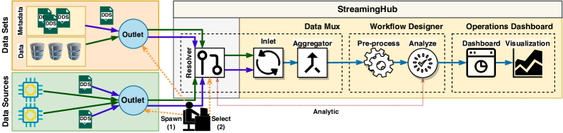
Figure 1. Component-level Overview of StreamingHub: The DataMux uses DDS metadata to convert data from connected sensors and datasets into data-streams. This data is then passed into the Workflow Designer to facilitate the design and execution of workflows. The results generated by running workflows are displayed in real-time on the Operations Dashboard.

3.1. Data Description System (DDS)

DDS is a collection of schemas to create metadata for describing data-sources, data-analytics, and data-sets. Data-source metadata provides attributes to describe data streams, such as their frequency and channels. Data-analytic metadata provides attributes to describe analytic data streams and their provenance (i.e., the hierarchy of transformations that lead to it). Data-set metadata provides attributes to describe the ownership, identification, provenance, and groups (i.e., viewpoints) of a dataset, and to reference a resolver script that maps stream-wise and/or group-wise queries into data. Table 1 provides a summary of the metadata attributes used in DDS.

Table 1. Summary of metadata attributes used in DDS

DATA SOURCE
info	version, timestamp, and checksum (for identification)
device	model, manufacturer, and category of data source
fields	dtype, name, and description of all fields
streams	information on all data streams generated from it
DATA ANALYTIC
info	version, timestamp, and checksum (for identification)
sources	pointer(s) to the data source metadata
fields	pointer(s) to the fields used in analysis
inputs	pointer(s) to the streams used in analysis
streams	information about all streams generated via analysis
DATA SET
info	version, timestamp, and checksum (for identification)
name	name of the data set
description	description of the data set
keywords	keywords describing the data set (for indexing)
authors	name, affiliation, and email of each data set author
sources	pointer(s) to the data source metadata
fields	pointer(s) to the fields used in analysis
groups	viewpoints to query different slices of the dataset
resolver	path to an executable that resolves data in the dataset

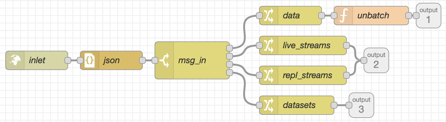
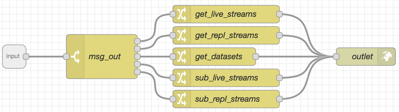
Figure 2. DataMux API Implemented on Node-RED: The DataMux In (left) sub-flow reads incoming messages from DataMux and routes them into the correct path in the workflow. The DataMux Out (right) sub-flow parses messages generated from the workflow and converts them into the format expected by DataMux.

3.2. DataMux

DataMux (see Figure 1) operates as a bridge between connected sensors, datasets, and data-streams. It uses DDS metadata to create the data-streams needed for a task, and supports three modes of execution:

• Live Mode – generate a data-stream that proxies live data from connected sensors (using data-source metadata)

• Replay Mode – generate a data-stream that replays a stored dataset (using data-source and data-set metadata)

• Simulate Mode – generate a data-stream of guided/unguided synthetic data (using data-source metadata)

In Live Mode, the DataMux uses LabStreamingLayer (GitHub, 2022) to interface with live data. The underlying functionality of each mode is encapsulated within a WebSocket API, i.e., the DataMux API. It serves as an interface to stream data into workflows and back.

Usage: The user first spawns the DataMux (server) on the local network, and opens a WebSocket connection to it. This DataMux connection is initially in awaiting state. Using this connection, the user can query for available live data-streams (which are generated from connected sensors in the local network) and replay data-streams (which are generated from datasets on the local file system). When queried for live data-streams, the DataMux discovers LabStreamingLayer outlets on the local network, and returns a list of them. When queried for replay data-streams, the DataMux first discovers DDS data-set metadata files on the local file system, and returns a list of their data-streams by calling the resolver script that each metadata file points to. From these returned data-streams, the user can subscribe to all or a subset of them, and start receiving their data. Note that data-stream discovery and subscription are kept independent to improve scalability. When a user subscribes to a data-stream, the DataMux connection transitions into streaming state, and spawns inlets to receive data. For live data-streams, each inlet connects to a LabStreamingLayer outlet, and proxies data from it in real-time. For replay data-streams, however, each inlet connects to one or more files in a dataset, and replays its data at the frequency it was recorded in. Next, data from these inlets pass through an aggregator which performs time-synchronization and merges data-streams where applicable. When merging data-streams, the aggregator adheres to the data frequencies specified in the metadata, to facilitate temporally-consistent replay and simulation. When the DataMux connection is in streaming state, the subscribed data-streams will continue streaming until the connection ends, or until the data-streams end.

3.3. Workflow Designer

The workflow designer is the visual programming front-end to build scientific workflows (see Figure 4 for an example). We use Node-RED to implement the workflow designer, as it offers a visual programming front-end to build workflows, while allowing users to import/export workflows in JSON format. This facilitates both technical and non-technical users to design workflows and share them among peers. We implemented a set of nodes to interface with the DataMux and made them available on the workflow designer. Workflows generated using this interface comprise of transformation nodes and visualization nodes that are bound in a directed graph using connectors. Transformation nodes define the operations performed on input data, and the output(s) generated from them. Each transformation node may accept multiple data streams as input, and may generate multiple data streams as output. Moreover, they propagate metadata from input data streams to output data streams, and append metadata about the transformation itself to preserve provenance. Visualization nodes, on the other hand, may accept multiple data streams as input, but instead of generating output streams, they generate visualizations. In this work, we primarily use Vega (Satyanarayan et al., 2015) to declare visualization nodes in JSON format. Additionally, a node itself can be defined as a workflow, allowing users to form hierarchies of workflows. This allows users to re-use existing workflows to form more complex workflows, which also serves as a form of abstraction (see Figure 2 for examples).

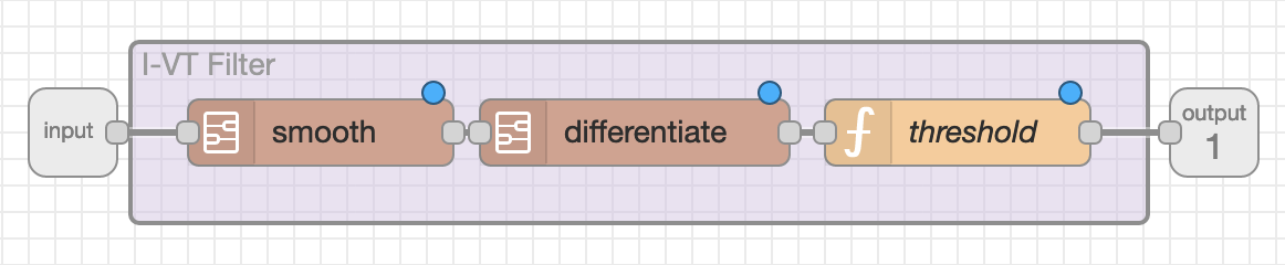
Figure 3. IVT sub-flow on Node-RED: Incoming gaze data first enters Smooth, which removes high-frequency noise via a Butterworth filter. Next, it enters Differentiate, which calculates first derivatives via a Savitzky-Golay filter. Next, it enters Threshold, which outputs fixation/saccade-labeled data using derivatives.

3.4. Operations Dashboard

The operations dashboard allows users to monitor active workflows, generate interactive visualizations, and perform data-stream control actions (see Figure 5 for a sample dashboard). We use Node-RED to implement the operations dashboard. When designing a workflow, users may add visualization nodes at any desired point in the workflow. Each visualization node, in turn, would generate a dynamic, reactive visualization on the operations dashboard. In terms of data-stream control, we propose to include five data-stream control actions: start, stop, pause, resume, and seek. These actions would enable users to navigate data streams temporally and perform visual analytics (Keim et al., 2008), a particularly useful technique to analyze high-frequency, high-dimensional data.

3.5. Platform Heuristics

As a part of this study, we propose two heuristics to quantify the workload in streaming workflows: 1) fluidity, a ratio of inbound to outbound data frequency, and 2) growth factor, a ratio of inbound to outbound data volume. These measures are similar in spirit to buffer underrun/overrun probability and packet jitter in streaming applications, with more contextual relevance to SWFs.

Fluidity (F): We propose Fluidity as a heuristic for computational bottlenecks in a transformation $T:S_{i}{\rightarrow}S_{o}$, where $S_{i}$ is the set of input streams, and $S_{o}$ is the set of output streams. Here, each $s_{o}\in S_{o}$ will have an expected frequency $f_{e}$, and a mean observed frequency $f_{\mu}$. Formally, we define Fluidity as,

$$F(s_{o},t)=1-\sqrt{1-({f_{\mu}}/{f_{e}})^{2}}$$

where, $F(s_{o},t)\in[0,1]$, and $f_{\mu}\in[0,f_{e}]$. For any output stream $s_{o}$, $f_{e}$ is constant, but $f_{\mu}$ varies with time. As $f_{\mu}$ decreases, the fluidity drops. For larger drops in $f_{\mu}$, the drop in fluidity is higher. The value of $f_{\mu}$ depends on factors including, but not limited to, hardware, concurrency, parallelism, and scheduling. Intuitively, $f_{\mu}$ can be estimated by computing the number of samples generated by $T$ in unit time. However, since this estimate can be noisy, a Kalman filter could be used. Overall, a fluidity $\ll 1$ is an indicator of computational bottlenecks, while a fluidity $\approx 1$ is an indicator of good performance. Bottlenecked transformations identified in this manner can be improved by either code-level optimization or executing in a faster runtime, which, in turn, would increase fluidity.

Growth Factor (GF): We propose Growth Factor as a heuristic for the change in data volume through a transformation $T:S_{i}{\rightarrow}S_{o}$, where $S_{i}$ is the set of input streams, and $S_{o}$ is the set of output streams. Formally, we define Growth Factor as,

$$GF(s_{i},s_{o})=\big{(}\sum\limits_{s{\in}S_{o}}{V(s)}\big{)}\big{/}\big{(}\sum\limits_{s{\in}S_{i}}{V(s)}\big{)}~{},~{}V(s)=f_{s}\sum\limits_{c_{i}}{w_{c_{i}}}$$

where, $GF(s_{i},s_{o})\in[0,\infty)$, and $V(s)\geq 0$. For any stream $s$, the data volume $V(s)$ is calculated using its frequency $f_{s}$, and the “word size” $w_{c_{i}}$ of each channel $c_{i}$ in $s$. Here, the word size $w_{c_{i}}$ represents the number of bits occupied by a sample of data from channel $c_{i}$ (e.g., if $c_{i}$ is of type int32, then $w_{c_{i}}=32$). Furthermore, $GF<1$ indicates a data compression, $GF>1$ indicates a data expansion, and $GF=1$ indicates no change. Intuitively, outputs from transformations with $GF<1$ are likely candidates for caching and transmitting over networks, as they output a lower volume of data than they receive.

4. Evaluation and Results

Using StreamingHub, we build two interactive stream analysis workflows in the domains of eye movement analysis (Jayawardena et al., 2020; Duchowski et al., 2020) and weather analysis (Dzodom et al., 2020). Here, different domains were used to test if StreamingHub generalizes across applications serving different scientific purposes. From this, we evaluate three aspects of StreamingHub.

• Can we use DDS metadata to replay stored datasets?

• Can we build workflows for domain-specific analysis tasks?

• Can we create domain-specific data visualizations?

Using three datasets, we evaluate StreamingHub on two distinct stream analysis tasks in the domains of eye movement analysis and weather analysis. Here, we describe our data source(s) using the proposed metadata format, and build stream processing workflows that leverage this metadata. Based on our observations, we discuss the utility of StreamingHub for data stream processing, and uncover challenges that inspire future work.

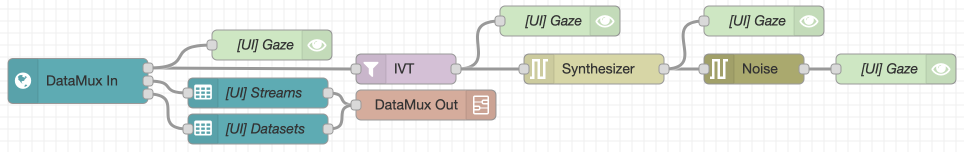
Figure 4. Eye movement analysis workflow on Node-RED: Gaze data from the DataMux In node enters an IVT node, which identifies fixations/saccades. This data enters a Synthesizer node, which synthesizes gaze data. Next, this data enters a Noise node, which adds Gaussian noise. The four [UI] Gaze nodes visualize gaze data, fixation/saccade data, synthetic gaze data, and noisy gaze data.

4.1. Eye Movement Analysis

4.1.1. Data Preparation

We use two existing datasets, ADHD-SIN (Jayawardena et al., 2020) and N-BACK (Duchowski et al., 2020), each providing gaze and pupillary measures of subjects during continuous performance tasks. We first pre-processed these datasets to provide normalized gaze positions (x,y) and pupil diameter (d) over time (t). Any missing values were filled via linear interpolation, backward-fill, and forward-fill, in order.

4.1.2. Experiment Design

In this experiment, we perform three tasks: 1) replay eye movement data, 2) obtain eye movement analytics in real-time, and 3) observe data/analytics through eye movement visualizations.

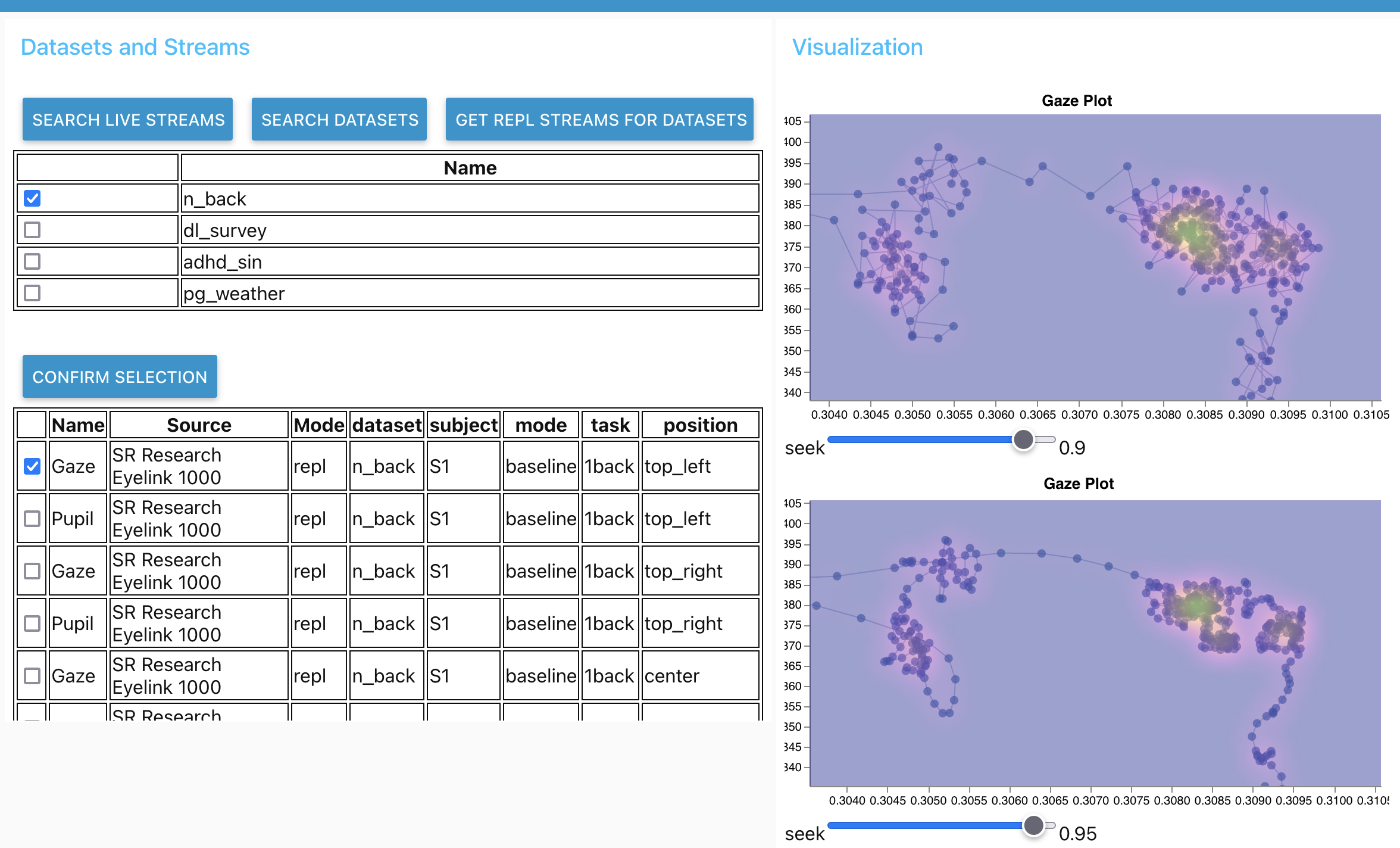
Figure 5. Operations Dashboard for Eye Movement Analysis: It visualizes, in real-time, raw (top-right) and synthesized (bottom-right) gaze data from replayed data (bottom-left) of the N-BACK dataset (top-left). The top-left buttons list available data-streams and datasets. The "Confirm Selection" button (mid-left) subscribes to selected data-streams and visualizes incoming data.

Task 1: Replay: We first generate DDS metadata for the N-BACK and ADHD-SIN datasets. Then we implement a resolver (using Python) for each dataset, which maps queries into respective data files, and references them in the metadata. Next, we use the DataMux API to list the data-streams of each dataset, and subscribe to them.

Task 2: Analytics: We create an eye movement analysis workflow on Node-RED, using visual programming. We begin by creating empty sub-flows for each transformation, and wiring them together, as shown in Figure 4. Next, we implement these sub-flows to form the complete workflow. For instance, we implement the I-VT algorithm (Salvucci and Goldberg, 2000) in the IVT sub-flow (see Figure 3) to classify data points as fixations or saccades.

Task 3: Visualization: We implement an interactive 2D gaze plot using the Vega JSON specification (Satyanarayan et al., 2015). It visualizes gaze points as a scatter plot, connects consecutive gaze points using lines, and overlays a heat map to highlight the distribution of gaze points across the 2D space. It also provides a seek bar to explore gaze data at different points in time. The resulting operations dashboard, as shown in Figure  5, displays the datasets and data-streams available for selection, the selected data-streams, and a real-time visualization of their data.

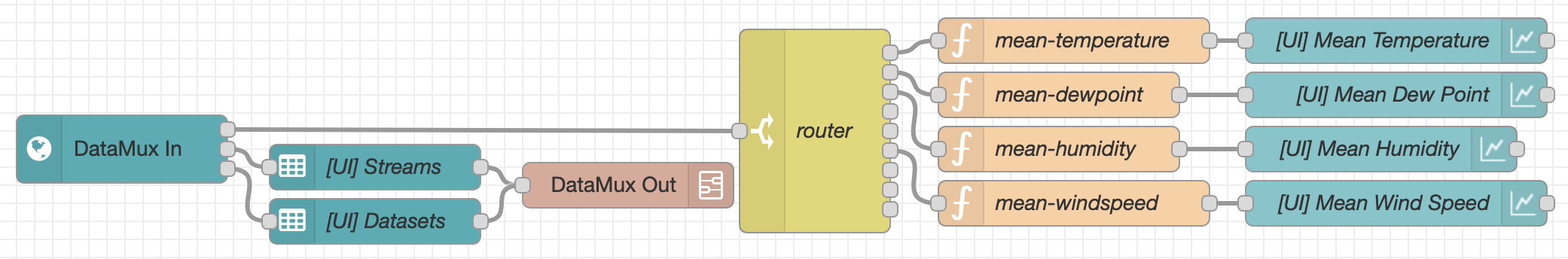
Figure 6. Weather analysis workflow on Node-RED: Weather data from the DataMux In node is passed into a Router node, which routes data (by type) into relevant visualization nodes. Only temperature, dew point, humidity, and wind speed data types are visualized.

4.2. Weather Analysis

4.2.1. Data Preparation

We use a dataset from PredictionGames (Dzodom et al., 2020) providing daily min/mean/max weather statistics (e.g., temperature, dew point, humidity, wind speed) of 49 US cities between 1950 and 2013. We first pre-processed this dataset by splitting weather data into seperate files by their city, and ordering records by their date.

4.2.2. Experiment Design

In this experiment, we perform three tasks: 1) replay weather data from different cities, 2) calculate moving average analytics in real-time, and 3) observe data/analytics through chart-based visualizations.

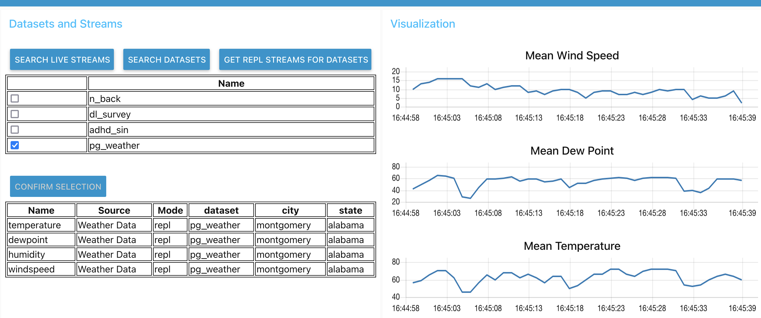
Figure 7. Operations Dashboard for Weather Analysis: It visualizes, in real-time, the mean values of wind speed, dew point, and temperature (right). All buttons and selection controls (left) offer the same functionality as described in Figure 5.

Task 1: Replay: We first create DDS metadata for the weather dataset. Here, we set the replay frequency as 1 Hz to speed up analysis (i.e., 1 day = 1 second). Then we implement a resolver (using Python) for this dataset, which maps queries into respective data files, and references them in the metadata. Next, we use the DataMux API to list the data-streams of the dataset, and subscribe to them.

Task 2: Analytics: We create a workflow to perform moving average smoothing on weather data and visualize each metric as shown in Figure 6. For the scope of this experiment, we only use the temperature, dew point, humidity, and wind speed metrics.

Task 3: Visualization: Here, we accumulate and visualize the averaged weather data through interactive charts. Figure 7 shows a snapshot of the operations dashboard while visualizing replayed weather data. It shows the datasets and data-streams available for selection, the selected data-streams, and a real-time visualization of their data.

Table 2. Mean latency ($\bar{t}$), inbound data size ($V_{i}$), and outbound data size ($V_{o}$) of four transformations ($T$) ranked by increasing compute demand ($D_{c}$) and outbound data size ($D_{s}$), in both REPLAY and LIVE modes.

$T$	$D_{c}$	$D_{s}$	$*$	REPLAY MODE			LIVE MODE
				$\bar{t}$ (ms)	$V_{i}$	$V_{o}$	$\bar{t}$ (ms)	$V_{i}$	$V_{o}$
Mean (Weather A)	1	1	w,s=50	0.018	782 MB	15.64 MB	0.024	782 MB	15.64 MB
Threshold (Eye Movement A)	2	2	I-VT filter (v=80)	0.097	782 MB	438 MB	0.132	782 MB	322.9 MB
Derivative (Eye Movement A)	3	4	int32$\rightarrow$float64	0.243	782 MB	1.54 GB	0.391	782 MB	1.54 GB
Smooth (Eye Movement A)	4	3	S-G filter (w=7)	0.645	782 MB	781.9 MB	0.726	782 MB	781.9 MB

In Table 2, we quantitatively assessed the performance of different sections of the workflows. We picked four transformations (i.e., nodes) from the workflows of both experiments, and ranked them in increasing order of their compute demand and outbound data size. Next, we sent 100,000 samples into each node at 50 Hz, and measured the mean latency $\bar{t}$, total inbound data size $V_{i}$, and total outbound data size $V_{o}$. We obtained these measurements in both replay and live modes (see Table 2).

Here, $\bar{t}$ was higher for all transformations in live mode, compared to replay mode. This may be due to differences in the underlying implementation; in live mode, data is proxied from devices using LabStreamingLayer whereas in replay mode, data is read (and cached) from files, and the frequency at which samples are replayed is regulated by a timer. This setup may be prone to I/O overhead, as seen in the results. Moreover, in both modes, the inbound and outbound data sizes are large since they are serialized in JSON format. In the future, we plan to use a space-efficient serialization format such as ProtoBuf to address this limitation.

5. Heuristic Evaluation

Here, we compare the proposed heuristics with the metrics reported in Table 2. For each transformation in this table, we send $100,000$ samples at $50\,Hz$, calculate the proposed heuristics, and compare our heuristics with the reported metrics. Based on our results, we determine if the proposed heuristics are consistent with the reported metrics.

Table 3. Comparison of performance metrics ($\bar{t}$, $V_{i}$, $V_{o}$) with heuristics ($F$, $GF$) for each transformation ($T$) on Table 2, in REPLAY mode.

$T$	$\bar{t}$ (ms)	$F$	$V_{i}$	$V_{o}$	$GF$
Mean	0.018	1.000	782 MB	15.64 MB	0.02
Threshold	0.097	0.999	782 MB	438 MB	–
Derivative	0.243	0.934	782 MB	1.54 GB	2.00
Smooth	0.645	0.742	782 MB	781.9 MB	1.00

Table 3 shows the mean latency $\bar{t}$ (ms), fluidity $F$, inbound data size $V_{i}$, outbound data size $V_{o}$, and growth factor $GF$ values obtained. For transformations with $F<1$, $\bar{t}$ was higher compared to transformations with $F=1$. Moreover, transformations with $V_{o}~{}\ll~{}V_{i}$ had $GF<1$; transformations with $V_{o}~{}\gg~{}V_{i}$ had $GF>1$; and transformations with a data-dependent $V_{o}$ had no $GF$ value.

Fluidity is based on observed frequency, and is not impacted by latency until throughput is affected. Furthermore, fluidity varies with time, but growth factor is independent of time. Thus, growth factor can be pre-calculated and used to dynamically optimize workflows for constrained resources. Moreover, both heuristics can be applied at transformation-level to determine which outputs to cache or re-generate. In this work, we only evaluated the proposed heuristics in replay mode, and not in live mode. A comprehensive evaluation should thus be performed to validate their utility across different applications.

6. Discussion

6.1. Societal Impact

One foreseeable application of this framework is to test experimental setups, both pre and post-collection. For pre-collection, one could simply stream in either random data or simulate test cases to verify that workflows run as expected. For post-collection, one could replay data through a workflow and verify that experimental results match. Overall, this provides an ecosystem to build robust, error-tolerant, and most importantly, reproducible real-time applications.

6.2. Limitations

In this study, our goal was to conceptualize metadata propagation and demonstrate how it facilitates reusable, reproducible analytics in scientific workflows with zero supervision. For this reason, our evaluation was focused on functionality and performance heuristics, and not user experience. In the future, we plan to conduct a user study to obtain feedback on (a) the workflow design experience and (b) the benefits of added reusability and reproducibility.

When developing our framework, we relied on the DDS metadata schema, which was purpose-built for metadata propagation. While creating DDS metadata for live data is relatively straightforward, doing so for stored data requires additional effort. In particular, it requires one to code resolver scripts that map queries to data. Despite being a one-time effort, this may limit the adoption of our framework outside real-time settings.

6.3. Future Work

Promoting Reuse: In this study, we implemented domain-specific sub-flows to execute our case studies (e.g., Fixation Detector, Gaze Synthesizer). In the future, we plan to refine these sub-flows and make them publicly available. Through this, we aim to promote the reuse of domain-specific workflows.

Improving Communication: In our framework, we used LabStreamingLayer to create, discover, and subscribe to data streams. In the future, we plan to explore alternative communication methods including, but not limited to, message brokers like MQTT (Hunkeler et al., 2008), and messaging protocols like protobuf (Blyth et al., 2019).

Time Synchronization: Our framework currently relies on LabStreamingLayer to synchronize different data streams in time. Internally, LabStreamingLayer uses the Precision Time Protocol (PTP) to perform this. In the future, we plan to implement such protocols as Node-RED sub-flows to promote flexibility and reuse.

Distributed Execution: At present, our framework only supports standalone workflow execution. In the future, we plan to integrate a workflow engine (e.g., Apache Flink, Amazon Kinesis) to enable distributed execution, and evaluate two aspects of it: workflow chaining (where analytic outputs of workflows are consumed by secondary workflows), and workload sharing (where components of workflows are executed across nodes) (see Figure 8). Moreover, since workload distribution is better optimized with knowledge of the underlying data, workload, and compute power (Isah et al., 2019), we plan to leverage fluidity and growth factor heuristics for such optimization.

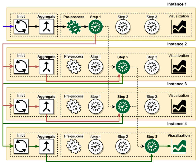
Figure 8. Distributed Execution of Workflows with workflow chaining (solid arrows) and workload sharing (dotted arrows).

7. Conclusion

We developed a framework (StreamingHub) to build stream analysis workflows that intelligently consume data, propagate metadata to downstream tasks, and thereby auto-generate reusable, reproducible analytic outputs with zero supervision. We also developed a metadata format (DDS) which facilitates metadata propagation in this framework, and proposed two heuristics to quantify computational aspects of a workflow built using it. We discussed how we implemented this framework using DDS, Node-RED, LabStreamingLayer, and WebSockets. We explained how it propagates metadata, and how it facilitates replaying datasets as data streams, passing data streams into workflows, performing data stream control, and conducting exploratory data analysis. We applied this framework for two case studies: eye movement analysis, and weather analysis. For eye movement analysis, we developed a workflow to detect fixations, simulate gaze data from fixations, and visualize gaze data. For weather analysis, we developed a workflow to visualize weather-related statistics, and replay data at different frequencies than recorded. We showed that the proposed heuristics indicate computational bottlenecks and estimate the expansion/compression of data in workflows. To promote reuse, our code is publicly available on https://github.com/nirdslab/streaminghub.

References

- (1)
- Akidau et al. (2015) Tyler Akidau, Robert Bradshaw, Craig Chambers, Slava Chernyak, Rafael J. Fernández-Moctezuma, et al. 2015. The Dataflow Model: A Practical Approach to Balancing Correctness, Latency, and Cost in Massive-Scale, Unbounded, Out-of-Order Data Processing. Proceedings of the VLDB Endowment 8 (2015), 1792–1803.
- Altintas et al. (2004) Ilkay Altintas, Chad Berkley, Efrat Jaeger, Matthew Jones, Bertram Ludascher, et al. 2004. Kepler: an extensible system for design and execution of scientific workflows. In Proceedings. 16th International Conference on Scientific and Statistical Database Management, 2004. IEEE, New York, NY, USA, 423–424.
- Alvarez-Coello et al. (2021) Daniel Alvarez-Coello, Daniel Wilms, Adnan Bekan, and Jorge Marx Gómez. 2021. Generic semantization of vehicle data streams. In 2021 IEEE 15th International Conference on Semantic Computing (ICSC). IEEE, New York, NY, USA, 112–117.
- Amazon Web Services (2022) Inc. Amazon Web Services. 2022. AWS Batch. Retrieved Apr 30, 2022 from https://aws.amazon.com/batch/
- Amstutz et al. (2016) Peter Amstutz, Michael R. Crusoe, Nebojša Tijanić, Brad Chapman, John Chilton, et al. 2016. Common Workflow Language, v1.0. https://doi.org/10.6084/m9.figshare.3115156.v2
- Avram (1968) Henriette D Avram. 1968. The MARC Pilot Project. Final Report. Technical Report. Library of Congress, Washington D.C.
- Bavoil et al. (2005) Louis Bavoil, Steven P Callahan, Patricia J Crossno, Juliana Freire, Carlos E Scheidegger, et al. 2005. Vistrails: Enabling interactive multiple-view visualizations. In VIS 05. IEEE Visualization, 2005. IEEE, New York, NY, USA, 135–142.
- Berthold et al. (2009) Michael R Berthold, Nicolas Cebron, Fabian Dill, Thomas R Gabriel, Tobias Kötter, et al. 2009. KNIME-the Konstanz information miner: version 2.0 and beyond. AcM SIGKDD explorations Newsletter 11, 1 (2009), 26–31.
- Bhardwaj et al. (2015) Anant Bhardwaj, Amol Deshpande, Aaron J. Elmore, David Karger, Sam Madden, et al. 2015. Collaborative Data Analytics with DataHub. Proceedings of the VLDB Endowment 8, 12 (2015), 1916–1919. https://doi.org/10.14778/2824032.2824100
- Blyth et al. (2019) David Blyth, J Alcaraz, Sébastien Binet, and Sergei V Chekanov. 2019. ProIO: An event-based I/O stream format for protobuf messages. Computer Physics Communications 241 (2019), 98–112.
- Brimhall and Vanegas (2001) G.H. Brimhall and A. Vanegas. 2001. Removing Science Workflow Barriers to Adoption of Digital Geologic Mapping by Using the GeoMapper Universal Program and Visual User Interface. In Digital Mapping Techniques. U.S. Geological Survey Open-File Report 01-223, Tuscaloosa, AL, USA, 103–115.
- Burnett and McIntyre (1995) Margaret M Burnett and David W McIntyre. 1995. Visual programming. COMPUTER-LOS ALAMITOS- 28 (1995), 14–14.
- Catlett et al. (2008) Charlie Catlett, William E Allcock, Phil Andrews, Ruth Aydt, Ray Bair, et al. 2008. Teragrid: Analysis of organization, system architecture, and middleware enabling new types of applications. In High performance computing and grids in action. IOS Press BV, Amsterdam, Netherlands, 225–249.
- Chintapalli et al. (2016) Sanket Chintapalli, Derek Dagit, Bobby Evans, Reza Farivar, Thomas Graves, et al. 2016. Benchmarking streaming computation engines: Storm, flink and spark streaming. In IEEE international parallel and distributed processing symposium workshops (IPDPSW). IEEE, New York, NY, USA, 1789–1792.
- Co. (2022) Neuromore Co. 2022. Neuromore. Retrieved Apr 30, 2022 from https://www.neuromore.com/
- Cundiff (2004) Morgan V Cundiff. 2004. An introduction to the metadata encoding and transmission standard (METS). Library Hi Tech 22, 1 (2004), 52–64. https://doi.org/10.1108/07378830410524495
- Deelman et al. (2015) Ewa Deelman, Karan Vahi, Gideon Juve, Mats Rynge, Scott Callaghan, et al. 2015. Pegasus: a Workflow Management System for Science Automation. Future Generation Computer Systems 46 (2015), 17–35. https://doi.org/10.1016/j.future.2014.10.008 Funding Acknowledgements: NSF ACI SDCI 0722019, NSF ACI SI2-SSI 1148515 and NSF OCI-1053575.
- Demšar et al. (2013) J. Demšar, T. Curk, A. Erjavec, Č. Gorup, et al. 2013. Orange: data mining toolbox in Python. The Journal of Machine Learning Research 14, 1 (2013), 2349–2353.
- Duchowski et al. (2020) Andrew T Duchowski, Krzysztof Krejtz, Nina A Gehrer, Tanya Bafna, and Per Bækgaard. 2020. The Low/High Index of Pupillary Activity. In Proceedings of the 2020 CHI Conference on Human Factors in Computing Systems. Association for Computing Machinery, New York, NY, USA, 1–12.
- Dumontier et al. (2016) Michel Dumontier, Alasdair JG Gray, M Scott Marshall, Vladimir Alexiev, Peter Ansell, et al. 2016. The health care and life sciences community profile for dataset descriptions. PeerJ 4 (2016), e2331.
- Dzodom et al. (2020) Gabriel Dzodom, Akshay Kulkarni, Catherine C Marshall, and Frank M Shipman. 2020. Keeping People Playing: The Effects of Domain News Presentation on Player Engagement in Educational Prediction Games. In Proceedings of the 31st ACM Conference on Hypertext and Social Media. Association for Computing Machinery, New York, NY, USA, 47–52.
- FAIRsharing (2022) FAIRsharing. 2022. FAIRSharing Standards. Retrieved Apr 30, 2022 from https://fairsharing.org/summary-statistics/
- Fegraus et al. (2005) Eric H Fegraus, Sandy Andelman, Matthew B Jones, and Mark Schildhauer. 2005. Maximizing the value of ecological data with structured metadata: an introduction to Ecological Metadata Language (EML) and principles for metadata creation. The Bulletin of the Ecological Society of America 86, 3 (2005), 158–168.
- Foster et al. (2008) Ian Foster, Yong Zhao, Ioan Raicu, and Shiyong Lu. 2008. Cloud computing and grid computing 360-degree compared. In 2008 grid computing environments workshop. IEEE, New York, NY, USA, 1–10.
- Foundation (2022) OpenJS Foundation. 2022. Node-RED. Retrieved Apr 30, 2022 from https://nodered.org/
- Fox (1992) Mary Frank Fox. 1992. Research, teaching, and publication productivity: Mutuality versus competition in academia. Sociology of education 65 (1992), 293–305.
- GitHub (2022) GitHub. 2022. Lab streaming layer (LSL). Retrieved Apr 30, 2022 from https://github.com/sccn/labstreaminglayer/
- Goble et al. (2020) Carole Goble, Sarah Cohen-Boulakia, Stian Soiland-Reyes, Daniel Garijo, Yolanda Gil, et al. 2020. FAIR computational workflows. Data Intelligence 2, 1-2 (2020), 108–121.
- Gorgolewski et al. (2011) Krzysztof Gorgolewski, Christopher D Burns, Cindee Madison, Dav Clark, Yaroslav O Halchenko, et al. 2011. Nipype: a flexible, lightweight and extensible neuroimaging data processing framework in python. Frontiers in neuroinformatics 5 (2011), 13.
- Hunkeler et al. (2008) Urs Hunkeler, Hong Linh Truong, and Andy Stanford-Clark. 2008. MQTT-S–A publish/subscribe protocol for Wireless Sensor Networks. In 2008 3rd International Conference on Communication Systems Software and Middleware and Workshops (COMSWARE’08). IEEE, New York, NY, USA, 791–798.
- Inc. (2022) Syntrogi Inc. 2022. NeuroPype. Retrieved Apr 30, 2022 from https://www.neuropype.io/
- Ioannidis et al. (2009) John PA Ioannidis, David B Allison, Catherine A Ball, Issa Coulibaly, Xiangqin Cui, et al. 2009. Repeatability of published microarray gene expression analyses. Nature genetics 41, 2 (2009), 149–155.
- Isah et al. (2019) Haruna Isah, Tariq Abughofa, Sazia Mahfuz, Dharmitha Ajerla, Farhana Zulkernine, et al. 2019. A survey of distributed data stream processing frameworks. IEEE Access 7 (2019), 154300–154316.
- Jayawardana and Jayarathna (2019) Yasith Jayawardana and Sampath Jayarathna. 2019. DFS: a dataset file system for data discovering users. In 2019 ACM/IEEE Joint Conference on Digital Libraries (JCDL). IEEE, New York, NY, USA, 355–356.
- Jayawardana and Jayarathna (2020) Yasith Jayawardana and Sampath Jayarathna. 2020. Streaming Analytics and Workflow Automation for DFS. In Proceedings of the ACM/IEEE Joint Conference on Digital Libraries in 2020. Association for Computing Machinery, New York, NY, USA, 513–514.
- Jayawardena et al. (2020) Gavindya Jayawardena, Anne Michalek, Andrew Duchowski, and Sampath Jayarathna. 2020. Pilot study of audiovisual speech-in-noise (sin) performance of young adults with adhd. In ACM Symposium on Eye Tracking Research and Applications. Association for Computing Machinery, New York, NY, USA, 1–5.
- Keim et al. (2008) Daniel Keim, Gennady Andrienko, Jean-Daniel Fekete, Carsten Görg, Jörn Kohlhammer, et al. 2008. Visual analytics: Definition, process, and challenges. In Information visualization. Springer, Cham, Switzerland, 154–175.
- King (2007) Gary King. 2007. An introduction to the dataverse network as an infrastructure for data sharing. Sociological Methods & Research 36, 2 (2007), 173–199.
- Kunze and Baker (2007) John Kunze and Thomas Baker. 2007. The Dublin core metadata element set. RFC 5013. Internet Engineering Task Force.
- Lagoze et al. (2008) Carl Lagoze, Herbert Van de Sompel, Michael L. Nelson, Simeon Warner, Robert Sanderson, et al. 2008. Object Re-Use & Exchange: A Resource-Centric Approach. arXiv:0804.2273 [cs.DL]
- Le Gruenwald (2005) Mihail Halatchev Le Gruenwald. 2005. Estimating missing values in related sensor data streams. Technical Report. University of Oklahoma.
- Lee and Neuendorffer (2000) Edward A Lee and Steve Neuendorffer. 2000. MoML — A Modeling Markup Language in XML - Version 0.4. Technical Report. University of California at Berkeley.
- Liew et al. (2016) Chee Sun Liew, Malcolm P Atkinson, Michelle Galea, Tan Fong Ang, Paul Martin, et al. 2016. Scientific workflows: moving across paradigms. ACM Computing Surveys (CSUR) 49, 4 (2016), 1–39.
- Malensek et al. (2011) Matthew Malensek, Sangmi Lee Pallickara, and Shrideep Pallickara. 2011. Galileo: A framework for distributed storage of high-throughput data streams. In 2011 Fourth IEEE International Conference on Utility and Cloud Computing. IEEE, New York, NY, USA, 17–24.
- Morrison (2010) J. Paul Morrison. 2010. Flow-Based Programming, 2nd Edition: A New Approach to Application Development. CreateSpace, Scotts Valley, CA.
- Nasiri et al. (2019) Hamid Nasiri, Saeed Nasehi, and Maziar Goudarzi. 2019. Evaluation of distributed stream processing frameworks for IoT applications in Smart Cities. Journal of Big Data 6, 1 (2019), 1–24.
- Nekrutenko and Taylor (2012) Anton Nekrutenko and James Taylor. 2012. Next-generation sequencing data interpretation: enhancing reproducibility and accessibility. Nature Reviews Genetics 13, 9 (2012), 667–672.
- Peng (2011) Roger D Peng. 2011. Reproducible research in computational science. Science 334, 6060 (2011), 1226–1227. https://doi.org/10.1126/science.1213847
- Pordes et al. (2007) Ruth Pordes, Don Petravick, Bill Kramer, Doug Olson, Miron Livny, et al. 2007. The open science grid. Journal of Physics: Conference Series 78 (July 2007), 012057. https://doi.org/10.1088/1742-6596/78/1/012057
- Prinz et al. (2011) Florian Prinz, Thomas Schlange, and Khusru Asadullah. 2011. Believe it or not: how much can we rely on published data on potential drug targets? Nature reviews Drug discovery 10, 9 (2011), 712–712.
- Roche et al. (2015) Dominique G Roche, Loeske EB Kruuk, Robert Lanfear, and Sandra A Binning. 2015. Public data archiving in ecology and evolution: how well are we doing? PLoS Biol 13, 11 (2015), e1002295.
- Rosenboom and Mullen (2019) David Rosenboom and Tim Mullen. 2019. More than one - Artistic explorations with multi-agent BCIs. In Brain Art. Springer, Cham, Switzerland, 117–143.
- Salvucci and Goldberg (2000) Dario D Salvucci and Joseph H Goldberg. 2000. Identifying fixations and saccades in eye-tracking protocols. In Proceedings of the 2000 symposium on Eye tracking research & applications. Association for Computing Machinery, New York, NY, USA, 71–78.
- Sandve et al. (2013) Geir Kjetil Sandve, Anton Nekrutenko, James Taylor, and Eivind Hovig. 2013. Ten simple rules for reproducible computational research. PLoS computational biology 9, 10 (2013), e1003285.
- Sansone et al. (2019) Susanna-Assunta Sansone, Peter McQuilton, Philippe Rocca-Serra, Alejandra Gonzalez-Beltran, Massimiliano Izzo, et al. 2019. FAIRsharing as a community approach to standards, repositories and policies. Nature biotechnology 37, 4 (2019), 358–367.
- Satyanarayan et al. (2015) Arvind Satyanarayan, Ryan Russell, Jane Hoffswell, and Jeffrey Heer. 2015. Reactive Vega: A Streaming DataFlow Architecture for Declarative Interactive Visualization. IEEE transactions on visualization and computer graphics 22, 1 (2015), 659–668.
- Sen and Duffy (2005) Marcus Sen and Tim Duffy. 2005. GeoSciML: development of a generic geoscience markup language. Computers & geosciences 31, 9 (2005), 1095–1103.
- Shukla et al. (2017) Anshu Shukla, Shilpa Chaturvedi, and Yogesh Simmhan. 2017. RIoTBench: An IoT benchmark for distributed stream processing systems. Concurrency and Computation: Practice and Experience 29, 21 (2017), e4257. https://doi.org/10.1002/cpe.4257
- Steen (2011) R Grant Steen. 2011. Retractions in the scientific literature: is the incidence of research fraud increasing? Journal of medical ethics 37, 4 (2011), 249–253.
- Thain et al. (2005) Douglas Thain, Todd Tannenbaum, and Miron Livny. 2005. Distributed computing in practice: the Condor experience. Concurrency and computation: practice and experience 17, 2-4 (2005), 323–356.
- Thelwall and Kousha (2016) Mike Thelwall and Kayvan Kousha. 2016. Figshare: a universal repository for academic resource sharing? Emerald Group Publishing Limited, UK.
- Towns et al. (2014) John Towns, Timothy Cockerill, Maytal Dahan, Ian Foster, Kelly Gaither, et al. 2014. XSEDE: accelerating scientific discovery. Computing in science & engineering 16, 5 (2014), 62–74.
- Van Dongen and Van den Poel (2020) Giselle Van Dongen and Dirk Van den Poel. 2020. Evaluation of stream processing frameworks. IEEE Transactions on Parallel and Distributed Systems 31, 8 (2020), 1845–1858.
- Van Mourik et al. (2018) Tim Van Mourik, Lukas Snoek, Tomas Knapen, and David G Norris. 2018. Porcupine: a visual pipeline tool for neuroimaging analysis. PLoS computational biology 14, 5 (2018), e1006064.
- Von Laszewski et al. (2010) Gregor Von Laszewski, Geoffrey C Fox, Fugang Wang, Andrew J Younge, Archit Kulshrestha, et al. 2010. Design of the futuregrid experiment management framework. In 2010 Gateway Computing Environments Workshop (GCE). IEEE, New York, NY, USA, 1–10.
- Wilkinson et al. (2016) Mark D Wilkinson, Michel Dumontier, IJsbrand Jan Aalbersberg, Gabrielle Appleton, Myles Axton, et al. 2016. The FAIR Guiding Principles for scientific data management and stewardship. Scientific data 3 (2016), 160018.
- Yasumoto et al. (2016) Keiichi Yasumoto, Hirozumi Yamaguchi, and Hiroshi Shigeno. 2016. Survey of real-time processing technologies of iot data streams. Journal of Information Processing 24, 2 (2016), 195–202.