Optimal Projection Filters

Abstract

We present the two new notions of projection of a stochastic differential equation (SDE) onto a submanifold, as developed in Armstrong, Brigo e Rossi Ferrucci (2019, 2018) [10, 9]: the Itô-vector and Itô-jet projections. This allows one to systematically and optimally develop low dimensional approximations to high dimensional SDEs using differential geometric techniques. Our new projections are based on optimality arguments and yield a well-defined “optimal” approximation to the original SDE in the mean-square sense. We also show that the earlier Stratonovich projection satisfies an optimality criterion that is more ad hoc and less natural than the criteria satisfied by the new projections. As an application, we consider approximating the solution of the non-linear filtering problem within a given manifold of densities, using either the Hellinger or $L^{2}$ direct metrics and related Information Geometry structures on the space of densities. The Stratonovich projection had yielded the projection filters studied in Brigo, Hanzon and Le Gland (1998, 1999) [20, 21], while the new projections lead to the optimal projection filters. The optimal projection filters have been introduced in [10], where numerical examples for the Gaussian case are given and where they are compared to more traditional nonlinear filters.

Keywords: Stochastic differential equations, Jets, SDEs projection on a submanifold, Stratonovich projection, Itô-vector projection, Itô-jet projection, Optimal Projection, Nonlinear Filtering, Projection Filters, Optimal Projection Filters.

AMS classification codes: 62M20, 93E11, 60G35, 62B10, 58J65, 60H10, 65D18, 58A20

1 Introduction and history

1.1 Information geometry as the differential geometric approach to statistics

Information Geometry is an informal term to describe the differential geometric approach to statistics, or more precisely to study the differential geometric properties of sets of probability distributions, on which a manifold structure is usually built, leading to so called statistical manifolds. The beginning of information geometry is usually attributed to the legendary mathematician and statistician, C. R. Rao, starting with his 1945 paper [49]. The theory has as one of its originating points the interpretation of the Fisher matrix for a parametric family of distributions as a Riemannian metric on the given finite-dimensional statistical manifold, the dimension being usually related to the number of parameters. The Fisher information matrix is related naturally to the Hellinger distance on more general infinite-dimensional spaces of probability measures, a distance based on the $L^{2}$ structure of sets of square roots of probability densities. Nand Lal Aggarwal (1974)[1], Shun'ichi Amari (1985) [3], Ole Barndorff-Nielsen (1978) [13] and Giovanni Pistone (Pistone and Sempi 1995 [48]) are key initial references, among others, that contributed to the development of information geometry.

1.2 Information geometry and filtering dynamics

Our work concerns the application of information geometry to approximation of dynamics of probability distributions, in most cases stemming from the stochastic filtering problem.

To state it in basic terms, in stochastic filtering one observes a random signal perturbed by random noise. The unperturbed random signal cannot be observed but needs to be estimated. For example, the perturbed signal could be the radar reading of the position of a spacecraft, which would not provide the exact position of the spacecraft due to several disturbances (“noise”) in the radar observations. It would then be necessary to estimate the real position of the spacecraft from the noisy radar readings. This is a filtering problem. A filtering algorithm was used in the Apollo 11 mission (Cipra 1993 [26]), the first human landing on the moon. Filtering has also applications in areas such as water level estimation and prediction, submarine navigation, econometrics, target tracking and many others. A good historical book on filtering with an eye to applications is Jazwinski (1970) [37], see also Maybeck (1982) [44], while the mathematical aspects are considered fully in Liptser and Shiryayev (1978) [42]. More recent monographs on filtering are Ahmed (1998) [2] and Bain and Crisan (2009) [12].

The general solution of the filtering problem at a given time is given by the probability density of the unperturbed state of the system at that time, conditional on the perturbed observations up to the given time. When the unobserved signal and the observed signal evolve in continuous time, the filter density follows a stochastic partial differential equation (SPDE). It has been shown that this probability density, the solution of the SPDE, does not evolve in a finite dimensional statistical manifold, except in very special cases. For example, if the dynamics of the unobserved system is linear, the observations are linear, the noises are Gaussian and the initial condition of the unperturbed signal is also Gaussian (or deterministic), then the filter is Gaussian and its density can be characterized by a finite dimensional set of parameters, namely the mean vector and variance-covariance matrix of the resulting Gaussian distribution. This leads to the celebrated Kalman filter. However, this does not happen usually, in the non-linear case, and the filter is infinite dimensional in general, as shown for the cubic sensor example by Hazewinkel, Marcus and Sussmann (1983) [35].

1.3 Classic projection filters: Stratonovich–Hellinger projection

Enters information geometry. Can information geometry provide us with a method to approximate the infinite-dimensional filter with a finite-dimensional approximation that is close to the original filter? The idea to apply the Fisher Metric and Hellinger distance to this problem was first sketched in an article of Bernard Hanzon (1987) [33] while he was working at the Technical University of Delft. Hanzon suggested to project the SPDE equation in Stratonovich form for the evolution of the filter density onto a finite dimensional statistical manifold, using the Fisher metric/Hellinger distance. We call this “Stratonovich projection” and it consists in projecting the separate vector fields of the SPDE corresponding to the drift and diffusion part of the Stratonovich version. The projected equation would describe a finite dimensional density evolution, called projection filter, approximating the full filter evolution associated with the optimal filter. The paper was presented to a key conference in Lancaster whose proceedings were edited by Christopher T. J. Dodson, in a volume with the almost prophetic title “Geometrization of Statistical Theory”. The following year, on August 22, 1988, Hanzon presented the idea at a seminar in Tokyo University called “The Projection Filter” while visiting Shun'ichi Amari. A few years later, in 1991, Hanzon and a PhD student Ruud Hut also from Technical University of Delft, wrote the paper Hanzon and Hut [32] with new results on the projection filter on Gaussian densities, showing that for the Gaussian family the projection filter coincides with a heuristic-based family of finite dimensional filters, the assumed density filters, previously studied by Harold Kushner (1967) [39], see also [44].

The projection filter idea was formulated precisely, extended and made fully rigorous in subsequent works, during the PhD studies of Damiano Brigo with Bernard Hanzon at the Free University of Amsterdam and with Francois LeGland at IRISA/INRIA, in Rennes, France, in 1993–1996 [17]. In these studies it was shown, among other things, that exponential families played a very particular role in the projection filter, allowing for the correction step of the filtering algorithm to be exact, and also fully generalizing the equivalence to the assumed density filters. The filters were tested numerically on some examples. During his PhD, Brigo also authored other papers on small observation noise for the Gaussian projection filter [16, 18] and on approximations of the Fokker-Planck-Kolmogorov equation, as well as formulations of the filter in discrete time using the Kullback Leibler information, with application to volatility modeling in finance [19]. The main results on the projection filters were published later in Brigo, Hanzon and LeGland (1998, 1999) [20, 21].

One of the key issues, from the start, was making sure that the given approximated equation for the filter density would stay on the chosen statistical manifold. The Stratonovich projection ensured this, but scholars had been studying the behaviour of stochastic differential equations on manifolds independently of the filtering application above. Among those, we refer to David Elworthy (1988) [27], Michel Emery (1989) [29], and more recently Elton Hsu (2002) [36]. We also notice that Elworthy, Le Jan and Li (2010) would discuss geometric aspects of filtering theory in [28], although their book does not deal with projection filters.

1.4 Classic projection filters: Stratonovich–direct $L^{2}$ projection

The cold war had ended, the military applications of filtering were receiving less and less funding, and many stochastic analysts who had previously worked on filtering turned to other areas, and many turned to mathematical finance. Brigo turned to a career in mathematical finance, but returned to the filtering problem as a side project in 2011 after he moved from a managing director position in the financial industry to a full academic position as Gilbart Chair at the Department of Mathematics of King’s College London, earlier in 2010. There, in 2011 he met a new colleague, John Armstrong, a differential geometry PhD from Oxford who had worked on almost Kähler geometry and who also had spent several years in the financial industry and was now turning to a full-time academic career. Brigo explained the filtering problem to Armstrong, who grasped immediately the essential ideas and the mathematics. Brigo had already written a preprint on his new idea of applying the direct $L^{2}$ structure without square roots to obtain a new type of projection filter, showing equivalence with Galerkin-based filters when using mixtures of distributions. Armstrong refined the idea and implemented the filter numerically, studying the cubic sensor problem. This led to a second wave of projection filters based on the direct $L^{2}$ metric as opposed to the Hellinger distance. It turned out that, as anticipated in the preprint, while the original Hellinger-based filters worked well with exponential families, being equivalent to assumed density filters, the direct $L^{2}$ filters worked best with mixture families, being equivalent to Galerkin-based filters. This research went on in 2011-2013 and was published in Armstrong and Brigo (2016) [6]. By 2012 Brigo had moved to Imperial College, so this had become a cooperation between the Mathematics Departments at King’s College London and Imperial College London. During the review of [6], one of the reviewers asked in which sense, or according to which criterion, the projection filter was providing an optimal approximation of the true filter. Armstrong immediately grasped the problem, while Brigo realized that while he had taken the Stratonovich projection for granted, he could not really tell in which sense it was optimal for the approximation of the true filter SPDE as a whole.

1.5 Is the classic projection filter an optimal approximation?

The essence of the problem of optimality of the approximation was based on the way the filtering equation was projected in the projection filter works published until then, mainly [20, 21, 6]. There are two stochastic calculi, Ito and Stratonovich. The two different calculi are suited to different applications, but from a probabilistic point of view the Ito calculus has a more clear interpretation of the stochastic equation coefficients in terms of local mean and local standard deviation, linked to the martingale property. Also, it is believed that even when one works with Stratonovich calculus, under the formalism one can argue that it is still the Ito calculus that “does all the work” (Rogers and Williams (1987) [50], Chapter V.30, p. 184). The problem with Ito calculus is that it violates the chain rule for change of variables. When changing variables, one has to use the famous Ito’s formula, involving a second order term in the transformation.

The true, infinite dimensional filter equation (taking the form of a stochastic partial differential equation, or SPDE) had always been written in Stratonovich form in the previous projection filter works, because in a Stratonovich stochastic equation the two parts describing the drift term and the diffusion coefficient term obey the chain rule under change of variables. This means that they can be interpreted as vector fields and be projected without problems on the tangent space of a submanifold, obtaining vector fields in the submanifolds that would form the approximating finite dimensional stochastic differential equation.

Projecting directly the Ito equation does not work, because the change of variables includes second order terms that do not resemble the behaviour of vector fields. Projection becomes then impossible to perform directly in Ito form. One could re-write the Ito true filter stochastic equation in Stratonovich form, project it, obtain a finite dimensional approximated filter, and transform back this approximate filter equation from Stratonovich to Ito form. But in what sense is this approximation optimal? What criterion does it minimize?

Brigo had never thought about this in depth because, in the back of his mind, he believed the projection of a vector field to always provide the best approximation of the original vector field. But a stochastic equation is given by two terms, the drift and the diffusion part, and if one puts the equation in Stratonovich form, the drift and the diffusion coefficients become described by two vector fields and as such can be projected. As the two vector fields are projected, each projected vector field will be the best approximation of the original vector field, but what does this mean for the solution of the stochastic equation as a whole? The stochastic equation is not just the pair of vector fields. In fact, when the equation is in Ito form, the drift and the diffusion coefficients interact when changing variables or coordinates, involving second order terms in the transformation. The fact that Stratonovich is “less good” probabilistically means that putting together two optimal projections of the coefficients to form a single Stratonovich equation does not provide a solution that is optimal in a probabilistic sense, for example in mean square.

1.6 Finding optimal projection filters

Armstrong had previously noticed that an Ito equation behaved exactly as a geometric object he was familiar with, called a 2-jet. Brigo, while helping Armstrong in developing the 2-jet interpretation of stochastic differential equations, started looking at the two other known ways to model stochastic equations in Ito form on manifolds, the Schwartz Morphism [29] and the Ito Bundle [14, 31], see also [25]. Focussing specifically on the Schwartz morphism, as studied in Emery (1989) [29], Brigo studied its relationship with the 2-jet approach and found them to be very close. The 2-jet interpretation was published in Armstrong and Brigo (2017, 2018) [7, 8], which led next to Armstrong and Brigo investigating how one could project a stochastic differential equation on a sub-manifold in an optimal way. Based on Ito Taylor expansions, two different projections satisfying two different types of optimality were found, the Ito-vector and the Ito-jet projections. The Ito-jet projection is superior in terms of optimality, in that it has a higher order of optimality in a precise sense. These results were presented at ICMS in Edinburgh by Armstrong and Brigo (2016) [5], at a conference co-organized in 2015 again by Dodson, almost thirty years after the original conference he had organized in Lancaster where the projection filter idea had first been presented. The ICMS conference was co-organized with Frank Critchley and Frank Nielsen. The two projections were studied further and some technical problems concerning tubular neighborhoods were solved with the help of the PhD student Emilio Rossi Ferrucci, leading to the publication Armstrong, Brigo and Rossi Ferrucci (2019) [10], see also Armstrong, Brigo and Rossi Ferrucci (2018) [9], where Rossi Ferrucci helped re-derive the optimal projections through constrained optimizations as opposed to Ito Taylor expansions, and where ambient coordinates are used.

In this last paper [10], information geometry comes back as an application of the now optimal projections both in Hellinger distance and direct $L^{2}$ metric, comparing them in a numerical case with the traditional Stratonovich projection of previous works. It turns out that Stratonovich is also optimal for a particular criterion that is, however, not a particularly interesting or natural one, so that the Ito-jet projection filter should be preferred in general.

In this paper we will first present a literature review of projection filtering as done by other authors, following the original papers [20, 21], and then we will detail the above history as much as possible, with derivations, equations and references. We will finally sketch future problems where information geometry might give a contribution. For the reader convenience, we summarize the different projection filtering approaches in Table 1.

Metric $\rightarrow$	Hellinger	Direct $L^{2}$
Projection $\downarrow$
Stratonovich	Stratonovich “classic” PF	Stratonovich “classic” PF
projection	exponential families [20, 21]	mixture families [6]
Ito-vector	Optimal Ito-vector PF	Optimal Ito-vector PF
projection	Gaussian familiy [10]	Gaussiam family [10]
	exponential families?	mixture families?
Ito-jet	Optimal Ito-jet PF	Optimal Ito-jet PF
projection	Gaussian familiy [10]	Gaussiam family [10]
	exponential families?	mixture families?

Table 1: A simplified classification of projection filters (PFs).

2 Other works based on the classic projection filters

Our original work on projection filters was further studied and applied to several fields by subsequent authors. Here we mention only a few examples to illustrate the breadth of the possible use of information geometry and dynamics in applications.

Eagle and Soatto (2011) [38] briefly mention the projection filter as one of the possible algorithms for on-line estimation in the context of visual-inertial navigation, mapping and localization. Lermusiaux (2006) [41] mentions the projection filter as a possible tool for estimation of uncertainties for ocean dynamics. Kutschireiter, Rast, and Drugowitsch (2022)[40] apply the projection filter to continuous time circular filtering. Projection filters have been applied to quantum systems for example in van Handel and Mabuchi (2005) [53] and in Gao, Zhang and Petersen (2019) [30]. Ma, Zhao, Chen and Chang (2015) [43] apply projection filters to hazard position estimation. Vellekoop and Clark (2006)[54] extend the projection filter theory to deal with changepoint detection. Tronarpand and Särkkä (2019) [52] present a projection filter for systems with discrete time measurement having arbitrary likelihoods. Surace and Pfister (2017) [51] apply the Gaussian projection filter to estimate the parameters of a partially observed diffusion. Harel, Meir and Opper (2015)[34] apply the assumed density filters, equivalent to the projection filters, to the filtering of optimal point processes with applications to neural encoding. Azimi-Sadjadi and Krishnaprasad (2005)[11] apply projection filter algorithms to navigation. Bröcker and Parlitz (2000)[24] apply projection filter techniques to address noise reduction in chaotic time series. Zhang, Wang, Wu and Xu (2014)[55] apply the Gaussian projection filter as part of their estimation technique to deal with measurements of fiber diameters in melt-blown nonwovens. The projection filter further attracted the attention of the Swedish Defense Research Agency, that summarized and studied it in 2003 in the report [15].

3 Optimal projection of stochastic differential equations

To study the optimal approximation of the filtering problem equation, we first introduce three different types of projections on submanifolds for SDEs. For simplicity we illustrate the differences with $n$-dimensional submanifolds $M$ of $\mathbb{R}^{r}$ but we will then apply this with $L^{2}$ replacing $\mathbb{R}^{r}$ and our chosen statistical manifold replacing $M$.

Figure 1 illustrates our SDE setting.

Here we will keep the exposition simple and will not provide all the mathematical details. The full exposition would require tubular neighborhoods, exit times, and constrained optimizations, see [9].

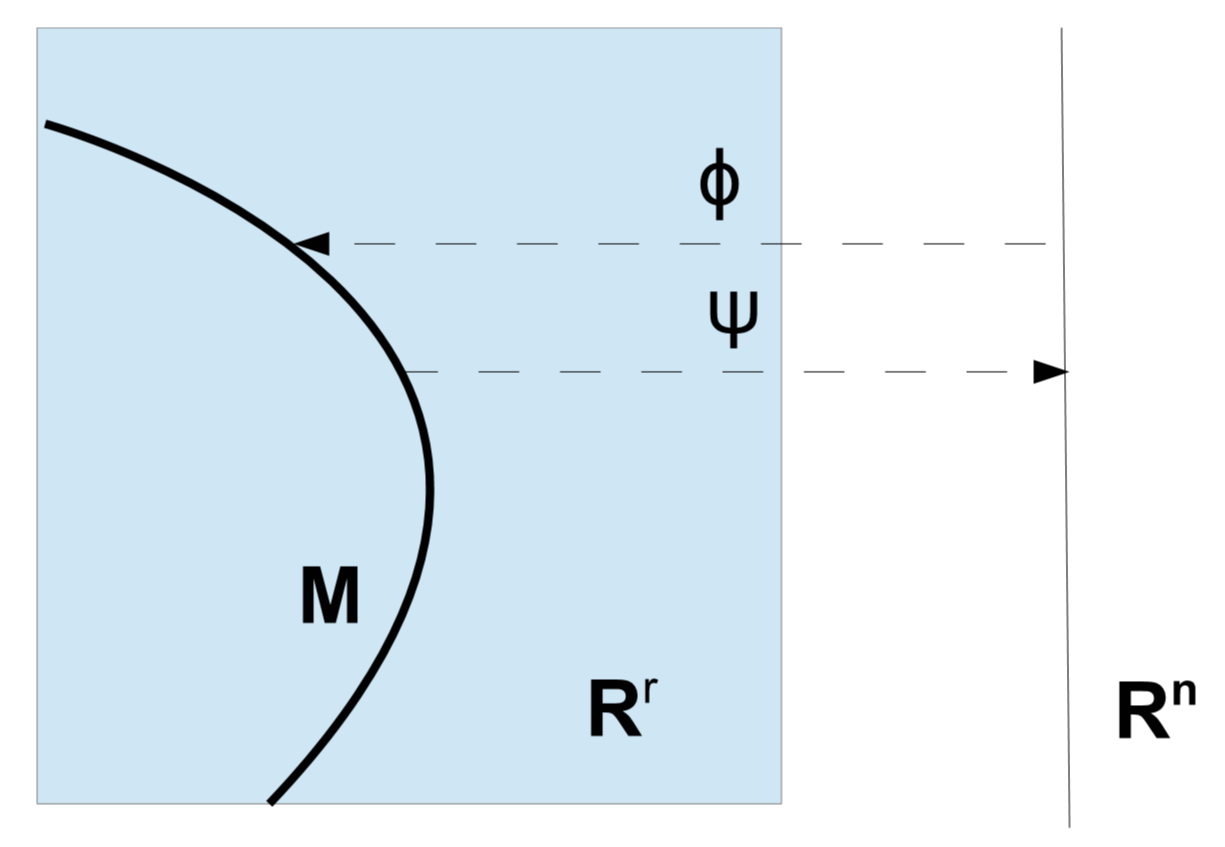
Figure 1: Approximate SDE
$dX=a(X)dt+b_{\alpha}(X)dW^{\alpha}$
in $\mathbb{R}^{r}$ with $\phi(Y)\in M$, where
$dY=A(Y)dt+B_{\alpha}(Y)dW^{\alpha}$
is SDE in $\mathbb{R}^{n}$, $X_{0}=\phi(Y_{0})\in M$, $n$-dimensional manifold of $\mathbb{R}^{r}$. $\psi$ is the specific chart, $\phi=\psi^{-1}$.

Our problem: given a SDE for $X$ on $\mathbb{R}^{r}$, $dX=a(X)dt+b_{\alpha}(X)dW^{\alpha}$ (Einstein convention applies, so $b_{\alpha}(X)dW^{\alpha}=\sum_{\alpha}b_{\alpha}(X)dW^{\alpha}$), with $M\subset\mathbb{R}^{r}$ an $n$-dimensional manifold of $\mathbb{R}^{r}$, and $X_{0}\in M$, we wish to find a SDE $\phi(Y)$ in $M$ starting at $\phi(Y_{0})=X_{0}$, $dY=A(Y)dt+B_{\alpha}(Y)dW^{\alpha}$ being the $\mathbb{R}^{n}$ coordinates SDE, whose solution approximates $X$ in some optimal way. Clearly, $r>n$. For brevity, we will often write $a$ for $a(X)$ and $b$ for $b(X)$, and similarly $A$ for $A(Y)$ and $B$ for $B(Y)$.

In the Stratonovich projection, the above Ito SDE is first transformed in Stratonovich form, obtaining the Stratonovich SDE for $X$ on $\mathbb{R}^{r}$,

$dX=\bar{a}(X)dt+b_{\alpha}(X)\circ dW^{\alpha}$, where $\bar{a}$ is the transformed drift for the Stratonovich version.

The full derivation of the optimal approximation and the theory on which this is based is given in full detail in Armstrong, Brigo and Rossi Ferrucci (2019, 2018)[10, 9], to which we refer for full details.

3.1 Stratonovich projection via tangent space projection

Figure 2: A pictorial representation of the tangent projection $\Pi$ of vector fields on a (red) circle that is used directly in the Stratonovich and Ito-vector projections.

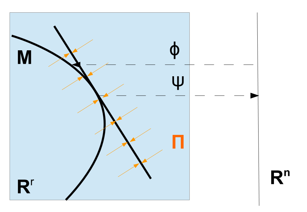
Figure 3: Stratonovich projection. Write the Ito SDE for $X$ in Stratonovich form
$dX=\bar{a}\ dt+b_{\alpha}\circ dW^{\alpha}\ \ \mbox{in}\ \ \mathbb{R}^{r}$,
$X_{0}\in M$. Apply the tangent space projection $\Pi$ on $M$ to obtain the $M$-SDE
for $Z=\phi(Y),Z_{0}=X_{0}$,
$dZ=\Pi_{Z}[\bar{a}]\ dt+\Pi_{Z}[b_{\alpha}]\circ dW^{\alpha}$

The Stratonovich projection is based on projection on the tangent space of the manifold $M$ of the vector fields $\bar{a}$ and $b_{\alpha}$’s. This is illustrated in Figure 3. For an expression in coordinates we have that the resulting Stratonovich projection SDE is $dY=\hat{A}(Y)dt+B_{\alpha}(Y)\circ dW^{\alpha}$ where

$$B_{\alpha}(Y_{t},t) = (\psi_{*})_{\phi(Y_{t})}\Pi_{\phi(Y_{t})}b_{\alpha}(\cdot,t),$$

$$\hat{A}(Y_{t},t) = (\psi_{*})_{\phi(Y_{t})}\Pi_{\phi(Y_{t})}\bar{a}(\cdot,t).$$

As one can see, in the Stratonovich projection we project the $dt$ and $dW_{t}$ vector fields separately, and get a new Stratonovich SDE that stays on the manifold. This is the projection that was used in the classic projection filter works (1987-2016) we mentioned in Sections 1.3 and 1.4. Also, all the references in Section 2 consider the Stratonovich projection filters. The use of the Stratonovich projection as a first method to derive a finite dimensional evolution equation is understandable, given its simplicity. One simply projects the two vector fields separately, and obtains automatically a new SDE on the submanifold. This is the main reason why one uses the Stratonovich projection. It also behaves well under change of coordinates, as coefficients are really vector fields.

However, given that Stratonovich SDEs do not behave as well as Ito SDEs probabilistically, what does this projection achieve for the SDE solution as a whole, rather than for the $dt$ and $dW$ vector fields taken separately? How do we justify the Stratonovich projection for $X$ as a whole?

Initially, when struggling with the problem of optimality, we thought the Stratonovich projection had no optimality. A first but somewhat weak justification for the Stratonovich projection is that for $b=0$ it coincides with the optimal ODE projection, minimizing the leading term of the Taylor expansion for $|\phi(Y)-X|^{2}$. However, if $b\neq 0$ and we are really dealing with a SDE rather than a ODE, is there any other sense where the Stratonovich projection is optimal? We found out there is a criterion, after all, for which this projection is optimal.

The Stratonovich projected SDE has a solution minimizing the leading ($t$-term) coefficient of the Taylor expansion of

$$\frac{1}{2}\left(\mathbb{E}[|{X_{-t}}-\phi(Y_{-t})|^{2}]+\mathbb{E}[|{X_{t}}-\phi(Y_{t})|^{2}]\right)$$

or of

$$\frac{1}{2}\left(\mathbb{E}[|{\pi(X_{-t})}-\phi(Y_{-t})|_{r}^{2}]+\mathbb{E}[|{\pi(X_{t})}-\phi(Y_{t})|_{r}^{2}]\right)$$

where $\pi$ is the metric projection from $\mathbb{R}^{r}$ on $M$, where in general if

$$d\xi_{t}=a(t,\xi_{t})dt+b_{\alpha}(t,\xi_{t})\circ dW^{\alpha}$$

then

$$\xi_{-t}:=\zeta_{t},\ \ d\zeta_{t}=-a(t,\zeta_{t})dt-b_{\alpha}(t,\zeta_{t})\circ d\bar{W}^{\alpha}$$

where $\bar{W}$ is a new Brownian motion independent of $W$. Clearly this is inspired by time symmetry, it is not very natural and is actually quite ad hoc, using time $0$ and the initial condition as an anchor point. This is not very helpful in practical applications. It is a somewhat artificial criterion of optimality that is not very interesting.

3.2 Ito-vector projection via tangent space projection

The idea of the Ito vector projection and the criterion it minimizes are summarized in Figure 4.

Figure 4: Itô vector projection. Minimize leading ($t$-term) coeff. of Taylor expansion of $\mathbb{E}[|{X_{t}}-\phi(Y_{t})|^{2}]$, to get $B$, but that coefficient does not vanish, so the error stays order $t$ rather than $t^{2}$. Fixing that $B$ in a neighborhood, get $A$ by minimizing the next leading term coeff ($t^{2}$-term). This results also in $A$ minimizing (regardless of $B$), up to order $t$, the weak error $|\mathbb{E}[{X_{t}}-\phi(Y_{t})]|^{2}$.

The coefficients $A$ and $B$ for the SDE on $\mathbb{R}^{n}$ such that $\phi(Y)$ is the Ito-vector projection of $X$ on $M$ are

$$B_{\alpha}(Y_{t},t)=(\psi_{*})_{\phi(Y_{t})}\Pi_{\phi(Y_{t})}b_{\alpha}(\cdot,t)\ \ \mbox{(same as Stratonovich proj.)}$$

$$A(Y_{t},t)=(\psi_{*})_{\phi(Y_{t})}\Pi_{\phi(Y_{t})}\left(a(\cdot,t)-\frac{1}{2}(\nabla_{B_{\alpha}(Y_{t},t)}\phi_{*})B_{\beta}(Y_{t},t)g^{\alpha\beta}_{E}\right).$$

The term $B$ is essentially the same as in the Stratonovich projection, consisting of the projection of the vector field $b$ on the tangent space of the manifold $M$.

The matrix $g^{\alpha,\beta}_{E}=1_{\{\alpha=\beta\}}$, or more generally it is the symmetric $2$-form defining the Euclidean metric on $\mathbb{R}^{m}$ in the non-orthonormal case. It may be helpful to recall that in Euclidean space notation (with orthonormal coordinates) we have

$$(\nabla_{B_{\alpha}}f_{i,\ast})B_{\beta}g^{\alpha,\beta}_{E}=\mbox{Trace}[B^{T}(Hf_{i})B]$$

with $H$ the Hessian operator. Given the drawback pointed out in Figure 4 of this projection being optimal only up to order $t$ rather than $t^{2}$, can we find another projection that, differently from the Itô vector projection, is consistently optimal up to order $t^{2}$?

The third and most optimal of the three projections will achieve this and will be based on the metric projection, rather than the tangent projection. A pictorial representation of the metric projection is presented in Figure 5.

3.3 Ito jet projection via metric projection

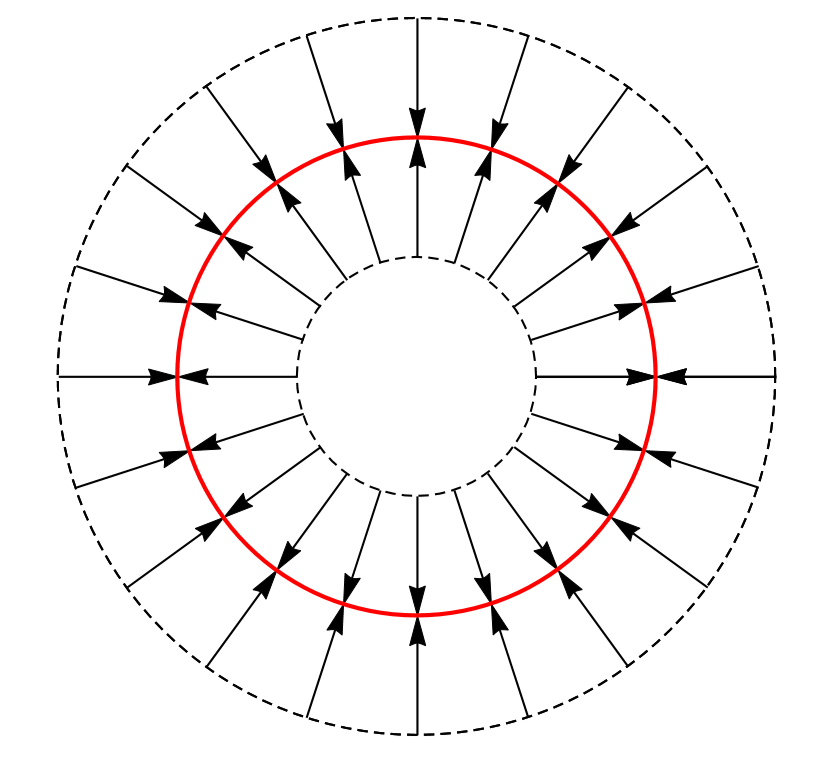
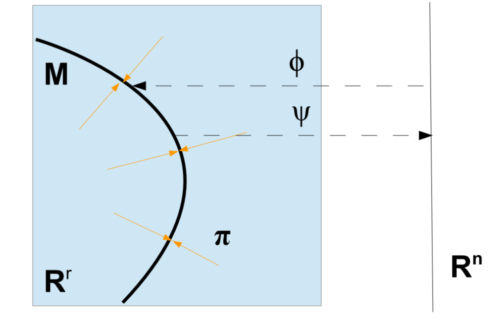
Figure 5: Above: A pictorial representation of the metric projection $\pi$ on a (red) circle $M$ that is used in the Ito-jet projection.
Below: $\pi$ is the metric projection
$\pi:\mathbb{R}^{r}\rightarrow M$,
defined on a tubular neighborhood of $M$, of which the earlier linear projection $\Pi$ is the first order component.
Using the chart $\psi$, set $\tilde{\pi}=\psi\circ\pi$. In the Itô jet projection we make the $t$ coefficient of the expansion vanish and minimize the leading $t^{2}$ coefficient of the Taylor expansion for the error $\mathbb{E}[d_{M}({\pi(X_{t})},\phi(Y_{t}))^{2}]$ or
$E[|{\pi(X_{t})}-\phi(Y_{t})|_{r}^{2}]$ for small $t$, so that we attain optimality up to order $2$. $d_{M}$ is the distance on $M$.

With this criterion, $B$ is as before, as in the Stratonovich and Ito vector projections, so we do not repeat it, while $A$ is given by

$$A(Y_{t},t)=\tilde{\pi}_{*}(a(\phi(Y_{t}),t))+\frac{1}{2}(\nabla_{b_{\alpha(\phi(Y_{t}),t)}}\tilde{\pi}_{*})b_{\beta}(\phi(Y_{t}),t)g^{\alpha\beta}_{E}.$$

In Armstrong, Brigo and Ferrucci-Rossi (2019) [10] we show the detailed calculations for $A$, which are very long and laborious. They involve the expansion of the metric projection. In short, define the metric tensor in a tubular neighborhood of $M$,

$$h_{ab}=\frac{\partial\phi^{\alpha}}{\partial x^{a}}\frac{\partial\phi^{\alpha}}{\partial x^{b}}$$ (1)

and call $h^{ab}$ the inverse of $h$. The differential ${\tilde{\pi}}_{*}$ of ${\tilde{\pi}}$ is well known to be given by the linear projection onto $\operatorname{Im}\phi_{*}$ composed with the map $\phi_{*}^{-1}$. Hence ${\tilde{\pi}}_{*}$ is the unique linear map with ${\tilde{\pi}}_{*}\circ\phi_{*}$ equal to the identity and with kernel equal to the orthogonal complement of $\operatorname{Im}\phi_{*}$. We deduce that ${\tilde{\pi}}_{*}$ has the following components:

$$\Pi^{a}_{b}:=({\tilde{\pi}}_{*})^{a}_{b}=\frac{\partial\phi^{b}}{\partial x^{\alpha}}h^{a\alpha},\qquad a\leq n,\alpha\leq n,b\leq r.$$ (2)

We note that the differential or tangent map ${\tilde{\pi}}_{*}$ is the best linear approximation of the metric projection ${\tilde{\pi}}$ around the relevant point $x=\phi(y)\in M$, and it coincides with the classic linear projection $\Pi_{\phi(y)}$ on the tangent space of $M$.

$$A^{i}=\Pi^{i}_{\alpha}a^{\alpha}+\left(-\frac{1}{2}\frac{\partial^{2}\phi^{\gamma}}{\partial x^{\alpha}\partial x^{\beta}}\Pi^{i}_{\gamma}\Pi^{\alpha}_{\delta}\Pi^{\beta}_{\epsilon}+\frac{\partial^{2}\phi^{\epsilon}}{\partial x^{\alpha}\partial x^{\beta}}\Pi^{\beta}_{\delta}h^{i\alpha}-\frac{\partial^{2}\phi^{\gamma}}{\partial x^{\alpha}\partial x^{\beta}}\Pi^{\beta}_{\epsilon}\Pi^{\eta}_{\gamma}\Pi^{\zeta}_{\delta}h_{\eta\zeta}h^{i\alpha}\right)\times b^{\delta}_{\kappa}b^{\epsilon}_{\iota}[W^{\kappa},W^{\iota}]_{t}.$$

We summarize the different projections and the optimality criteria used to determine their drifts in Table 2 in the conclusions. The diffusion coefficient is identical for all three projections.

4 Application to Non-linear Filtering via Information Geometry

We studied the application of the new projections to nonlinear filtering via information geometry in Armstrong, Brigo and Rossi Ferrucci (2019) [10]. Here we summarize the results of that paper, showing how our new projection methods work for stochastic filtering. As explained in the introduction, this enhances optimality of the approximations compared to our previous works in [20], [21] and [6].

Let us first summarize the filtering problem for diffusions. One has a signal $X$ that evolves according to a SDE, and observes a process $Y$ which is a function of this signal plus noise. This is standard notation, but these $X$ and $Y$ are not to be confused with the processes we used earlier in the paper, in that they are not the $\mathbb{R}^{r}$ process to be approximated and its $\mathbb{R}^{n}$ approximation.

The filtering problem consists in estimating the signal $X$ given the present and past observations $Y$. If $t$ is the current time, the solution of the filtering problem is the probability density of the state $X_{t}$ conditional on the observations from time 0 to time $t$, call this density $p_{t}$. The density $p_{t}$ follows the Kushner-Stratonovich (or alternatively the Zakai) stochastic partial differential equation (SPDE) that, under some technical assumptions, can be seen as a stochastic differential equation in the infinite dimensional $L^{2}$ space of square roots of densities (Hellinger metric) or of densities themselves (direct $L^{2}$ metric).

The process we wish to approximate on a low dimensional manifold is $p_{t}$, which represents the $X_{t}$ of our earlier sections. The $\mathbb{R}^{r}$ space of our earlier sections is the $L^{2}$ infinite dimensional space, while the submanifold $M$ is a finite dimensional family of probability densities parametrized by $\theta$, acting as coordinates: $\{p(\cdot,\theta),\ \theta\in\Theta\subset\mathbb{R}^{n}\}$. $\theta_{t}$ plays the role of what we were calling $Y_{t}$ earlier in the paper. For brevity, we will often omit the argument and write $p(\cdot,\theta)=p_{\theta}$. We aim at finding a SDE for $\theta$ such that $p_{\theta_{t}}$ approximates the optimal filter $p_{t}(\cdot)$ in an optimal way. Note that in the previous part of the paper we had a dimensionality reduction from $r$ to $n$, whereas now we go from infinite dimensional $p_{t}$ to $n$-dimensional $\theta_{t}$.

We discuss in [10] how the setting can be generalized from $\mathbb{R}^{r}$ to $L^{2}$.

4.1 The Kushner Stratonovich equation

We suppose that the state $X_{t}\in\mathbb{R}^{m}$ of a system evolves according to the equation:

$$\mathrm{d}X_{t}=f(X_{t},t)\,\mathrm{d}t+\sigma(X_{t},t)\,\mathrm{d}W_{t}$$

where $f$ and $\sigma$ are smooth $\mathbb{R}^{m}$ valued functions and $W_{t}$ is a Brownian motion. One typically adds growth conditions to ensure a global existence and uniqueness result for the signal equation, see for example [6] and references therein for the details.

We suppose that an associated process, the observation process, $Y_{t}\in\mathbb{R}^{d}$ evolves according to the equation:

$$\mathrm{d}Y_{t}=b(X_{t},t)\,\mathrm{d}t+\mathrm{d}V_{t}$$

where $b$ is a smooth $\mathbb{R}^{d}$ valued function and $V_{t}$ is a Brownian motion independent of $W_{t}$. Note that the filtering problem is often formulated with an additional constant in terms of the observation noise. For simplicity we have assumed that the system is scaled so that this can be omitted.

The filtering problem is to compute the conditional distribution of $X_{t}$ given a prior distribution for $X_{0}$ and the values of $Y$ for all times up to and including $t$.

Subject to various bounds on the growth of the coefficients of this equation, the assumption that the distribution has a density $p_{t}$ and suitable bounds on the growth of $p_{t}$ one can show that $p_{t}$ satisfies the Kushner–Stratonovich SPDE:

$$\mathrm{d}p={\cal L^{*}}p\ \mathrm{d}t+p[b-E_{p}(b)]^{T}[\mathrm{d}Y-E_{p}(b)\mathrm{d}t]$$ (3)

where $E_{p}$ denotes the expectation with respect to the density $p$,

$E_{p}[f]=\int f(x)p(x)dx$, and the forward diffusion operator ${\cal L}^{*}_{t}$ is defined by:

$${\cal L}_{t}^{*}\phi=-\frac{\partial}{\partial x^{i}}[f_{i}(x,t)\phi]+\frac{1}{2}\frac{\partial^{2}}{\partial x^{i}\partial x^{j}}[a_{ij}(x,t)\phi]$$ (4)

where $a=\sigma\sigma^{T}$. Note that we are using the Einstein summation convention in this expression.

In the event that the coefficient functions $f$ and $b$ are all linear and $\sigma$ is a deterministic function of time one can show that so long as the prior distribution for $X$ is Gaussian, or deterministic, the density $p$ will be Gaussian at all subsequent times. This allows one to reduce the infinite dimensional equation (3) to a finite dimensional stochastic differential equation for the mean and covariance matrix of this normal distribution. This finite dimensional problem solution is known as the Kalman filter.

For more general coefficient functions, however, equation (3) cannot be reduced to a finite dimensional problem [35]. Instead one might seek approximate solutions of (3) that belong to some given statistical family of densities. This is a very general setup and includes, for example, approximating the density using piecewise linear functions to derive a finite difference approximation or approximating the density with Hermite polynomials to derive a spectral method. Other examples include exponential families (considered in [21, 20]) and mixture families (considered in [4, 6]).

Our projection theory tells us how one can find good approximations on a given statistical family with respect to a given metric on the space of distributions. We illustrate this by writing down the Itô-vector and Itô-jet projection of (3) for the $L^{2}$ and Hellinger metrics onto a general manifold.

We will then examine some numerical results regarding the very specific case of seeking approximate solutions using Gaussian distributions. The idea of approximating the solution to the filtering problem using a Gaussian distribution has been considered by numerous authors who have derived variously, the extended Kalman filter [47], assumed density filters [39] and Stratonovich projection filters [20]. Some of these are related, for example the assumed density filters and Stratonovich projection filters in Hellinger metrics for Gaussian (and more generally exponential) families coincide [21]. Using our new projection methods, we will be able to derive projection filters which outperform all these other filters (assuming performance is measured over small time intervals using the appropriate Hilbert space metric).

We note that (3) is an infinite dimensional SDE driven by a continuous semi-martingale. The definitions and results given in Section 3 were only stated in the finite dimensional case for SDEs driven by Brownian motion. The definition of Itô–Taylor series can be generalized straightforwardly to this situation and hence the definition of the Itô projections can be applied in this context also.

More generally, for the the geometry of approximations to the infinite dimensional filtering problems based on $L^{2}$ or Orlicz charts we refer for example to [20, 21, 6, 10, 22, 23, 45, 46].

4.2 Stratonovich projections

The Stratonovich projection filters have been abundantly studied in [20, 21] in Hellinger metric, and in [6] in direct metric, see also references in Section 2 for the Hellinger case. Here we briefly summarize them. For this method, the optimal filter SPDE is given by putting the optimal filter equation (3) in Stratonovich form, obtaining

$$dp={\cal L}^{\ast}\,p\,dt-\frac{1}{2}\,p\,[|b|^{2}-E_{p}\{|b|^{2}\}]\,dt+p\,[b-E_{p}\{b\}]^{T}\circ dY\ .$$ (5)

4.2.1 Stratonovich projection filter in $L^{2}$ direct metric

We use first the $L^{2}$ direct metric, by assuming densities are squared integrable, and view densities are elements of $L^{2}$ with the related inner product. For a discussion on conditions under which a unnormalized version of the density $p_{t}$ of the optimal filter (3) is in $L^{2}$ (Zakai Equation) see for example [2].

In the case of two probability density functions $p(x)$ and $q(x)$ on $\mathbb{R}^{m}$, we assume them to be in $L^{2}$, and the $L^{2}$ squared direct distance is

$$\int({p(x)}-{q(x)})^{2}\,\mathrm{d}x.$$

We wish to consider an $n$-dimensional family of distributions $p_{\theta}$ parameterized by $n$ real valued parameters $\theta^{1}$, $\theta^{2}$, $\ldots$, $\theta^{n}$. For example, for a scalar state space $x$, one may consider the 2 dimensional Gaussian family:

$$p_{\theta}(x)=\frac{1}{(\theta^{2})\sqrt{2\pi}}\exp\left(-\frac{(x-(\theta^{1}))^{2}}{2(\theta^{2})^{2}}\right).$$ (6)

For more general exponential or mixture families see [20, 21, 6]. Note that we have chosen to follow the differential geometry convention and use upper indices for the coordinate functions $\theta^{i}$ so we have been careful to distinguish powers from indices using brackets.

Once the family is chosen, in the Stratonovich projection we can project directly the $dt$ and the $dY$ terms of the optimal filter equation (5) on the tangent space of the chosen manifold $p_{\theta}$ in direct metric, as both terms behave as vector fields.

More formally, an $n$-dimensional family is given by a smooth embedding $\phi:\mathbb{R}^{n}\rightarrow L^{2}(\mathbb{R}^{m})$. The tangent vectors $\phi_{*}\frac{\partial}{\partial\theta^{i}}\in L^{2}(\mathbb{R}^{m})$ are simply the partial derivatives

$$\frac{\partial p_{\theta}}{\partial\theta^{i}}.$$

Let us write:

$$g_{ij}(\theta)=\int_{\mathbb{R}^{m}}\frac{\partial p_{\theta}(x)}{\partial\theta^{i}}\frac{\partial p_{\theta}(x)}{\partial\theta^{j}}\,\mathrm{d}x.$$

This defines the induced metric tensor on the manifold $\phi(\mathbb{R}^{n})$. We will write $g^{ij}$ for the inverse of the matrix $g_{ij}$. The projection operator $\Pi_{\phi(\theta)}$ is then given by

$$\begin{split}\Pi_{\phi(\theta)}(v)&=\sum_{i,j=1}^{n}g^{ij}(\theta)\left\langle v,\phi_{*}\frac{\partial}{\partial\theta^{i}}\right\rangle_{L^{2}}\phi_{*}\frac{\partial}{\partial\theta^{j}}\\ &=\sum_{i,j=1}^{n}g^{ij}(\theta)\left(\int_{\mathbb{R}^{m}}v(x)\frac{\partial p_{\theta}(x)}{\partial\theta^{i}}\,\mathrm{d}x\right)\phi_{*}\frac{\partial}{\partial\theta^{j}}\,.\end{split}$$

Thus

$$\phi_{*}^{-1}\Pi_{\phi(\theta)}(v)=\sum_{i,j=1}^{n}g^{ij}(\theta)\left(\int_{\mathbb{R}^{m}}v(x)\frac{\partial p_{\theta}}{\partial\theta^{i}}\,\mathrm{d}x\right)\frac{\partial}{\partial\theta^{j}}\,.$$

We can now write down the Stratonovich projection of (5) with respect to the $L^{2}$ metric. It is:

$$\mathrm{d}\theta^{i}=\hat{A}^{i}(\theta)\,\mathrm{d}t+B^{i}(\theta)\circ\,\mathrm{d}Y_{t}$$

where:

$$B^{i}(\theta)=\sum_{j=1}^{n}g^{ij}(\theta)\left(\int_{\mathbb{R}^{m}}(p_{\theta}(x)(b(x)-E_{p_{\theta}}(b)))^{T}\frac{\partial p_{\theta}(x)}{\partial\theta^{j}}\,\mathrm{d}x\right)$$

and

$$\hat{A}^{i}(\theta)=\sum_{j=1}^{n}g^{ij}(\theta)\left(\int_{\mathbb{R}^{m}}\left({\cal L}^{*}p_{\theta}-\frac{1}{2}p_{\theta}(|b|^{2}-E_{p_{\theta}}[|b|^{2}])\right)\frac{\partial p_{\theta}}{\partial\theta^{j}}\,\mathrm{d}x\right).$$

4.2.2 Stratonovich projection filter in Hellinger metric

If we use instead projection under the Hellinger distance, we need to work with square roots of densities. Indeed, the Hellinger metric is a metric on probability measures. In the case of two probability density functions $p(x)$ and $q(x)$ on $\mathbb{R}^{m}$, that now need only be in $L^{1}$, the Hellinger distance is given by the square root of:

$$\frac{1}{2}\int(\sqrt{p(x)}-\sqrt{q(x)})^{2}\,\mathrm{d}x.$$

In other words, up to the constant factor of $\frac{1}{2}$ the Hellinger metric corresponds to the $L^{2}$ norm on the square root of the density function rather than on the density itself (as in the previous case of the direct metric). The Hellinger metric has the important advantage of making the metric independent of the particular background density that is used to express measures as densities. The $L^{2}$ direct distance introduced earlier does not satisfy this background independence.

To get the equation for the square root of the optimal filter density $p$, we can now use the chain rule, as Stratonovich calculus satisfies it. We get

$$d\sqrt{p}=\frac{1}{2\sqrt{p}}\circ\ dp$$

or

$$d\sqrt{p}=\frac{1}{2\sqrt{p}}{\cal L}^{\ast}\,p\,dt-\frac{1}{4}\,\sqrt{p}\,[|b|^{2}-E_{p}\{|b|^{2}\}]\,dt+\frac{1}{2}\sqrt{p}\,[b-E_{p}\{b\}]^{T}\circ dY\ .$$ (7)

A family of distributions now corresponds to an embedding $\phi$ from $\mathbb{R}^{n}$ to $L^{2}(\mathbb{R}^{m})$ but now $p_{\theta}=\phi(\theta)^{2}$. The tangent space is spanned by the vectors:

$$\phi_{*}\frac{\partial}{\partial\theta^{i}}=\frac{\partial\sqrt{p_{\theta}}}{\partial\theta^{i}}.$$

We define a metric on the tangent space by:

$$h_{ij}(\theta)=\int_{\mathbb{R}^{m}}\frac{\partial\sqrt{p_{\theta}(x)}}{\partial\theta^{i}}\frac{\partial\sqrt{p_{\theta}(x)}}{\partial\theta^{j}}\,\mathrm{d}x.$$

We write $h^{ij}$ for the inverse matrix of $h_{ij}$. The projection operator with respect to the Hellinger metric is:

$$\begin{split}\Pi_{\phi(\theta)}(v)&=\sum_{i,j=1}^{n}h^{ij}(\theta)\left(\int_{\mathbb{R}^{m}}v(x)\frac{\partial\sqrt{p_{\theta}(x)}}{\partial\theta^{i}}\,\mathrm{d}x\right)\phi_{*}\frac{\partial}{\partial\theta^{j}}.\end{split}$$

We can now write down the Stratonovich projection of (7) with respect to the Hellinger metric. It is:

$$\mathrm{d}\theta^{i}=\hat{A}^{i}(\theta)\,\mathrm{d}t+B^{i}(\theta)\,\circ\mathrm{d}Y_{t}$$

where:

$$B^{i}(\theta)=\sum_{j=1}^{n}h^{ij}(\theta)\left(\int_{\mathbb{R}^{m}}\frac{1}{2}\sqrt{p_{\theta}(x)}(b(x)-E_{p_{\theta}}(b))^{T}\frac{\partial\sqrt{p_{\theta}(x)}}{\partial\theta^{j}}\,\mathrm{d}x.\right)$$

and

$$\hat{A}^{i}(\theta)=\sum_{j=1}^{n}h^{ij}(\theta)\left(\int_{\mathbb{R}^{m}}\left(\frac{{\cal L}^{*}p_{\theta}(x)}{2\sqrt{p_{\theta}(x)}}-\frac{1}{4}\,\sqrt{p_{\theta}(x)}\,[|b(x)|^{2}-E_{p_{\theta}}\{|b|^{2}\}]\right)\frac{\partial\sqrt{p_{\theta}(x)}}{\partial\theta^{j}}\,\mathrm{d}x.\right).$$

This is the Stratonovich SDE for $\theta_{t}$, the Stratonovich projection of the optimal filter on our family $p_{\theta}$ in Hellinger metric.

In the next sections we will derive the optimal Ito projections. These will be somehow more complicated and we will thus omit functions arguments such as $\theta$ and $x$ where obvious.

4.3 Itô-vector projections

4.3.1 The Itô-vector projection filter in the $L^{2}$ direct metric

Let us suppose again that the optimal filter density $p$ lies in $L^{2}$ and so we can use the $L^{2}$ norm to measure the accuracy of an approximate solution to equation (3).

We can now write down the Itô-vector projection of (3) with respect to the $L^{2}$ metric. It is:

$$\mathrm{d}\theta^{i}=A^{i}\,\mathrm{d}t+B^{i}\,\mathrm{d}Y_{t}$$

where:

$$B^{i}=\sum_{j=1}^{n}g^{ij}\left(\int_{\mathbb{R}^{m}}(p(b-E_{p(\theta)}(b)))^{T}\frac{\partial p}{\partial\theta^{j}}\,\mathrm{d}x\right)$$

and

$$A^{i}=\sum_{j=1}^{n}g^{ij}\left(\int_{\mathbb{R}^{m}}\left({\cal L}^{*}p-p(b-E_{p(\theta)}(b))^{T}E_{p(\theta)}(b)-\frac{1}{2}\sum_{k=1}^{n}\frac{\partial^{2}p}{\partial\theta^{j}\partial\theta^{k}}B^{k}\right)\frac{\partial p}{\partial\theta^{j}}\,\mathrm{d}x\right).$$

4.3.2 The Itô-vector projection filter in the Hellinger metric

Now, to compute the Itô-vector projection with respect to the Hellinger metric we first want to write down an Itô equation for the evolution on $\sqrt{p}$.

Applying Itô’s lemma to equation (3) we formally obtain:

$$\begin{split}\mathrm{d}\sqrt{p}&=\left(\frac{{\cal L}^{*}p-p(b-E_{p}(b))^{T}E_{p}(b)}{2\sqrt{p}}-\frac{p^{2}(b-E_{p}(b))^{T}(b-E_{p}(b))}{8p\sqrt{p}}\right)\,\mathrm{d}t\\ &{}+\left(\frac{p(b-E_{p}(b))^{T}}{2\sqrt{p}}\right)\mathrm{d}Y_{t}.\\ &=\left(\frac{{\cal L}^{*}p}{2\sqrt{p}}-\frac{1}{8}\sqrt{p}(b-E_{p}(b))^{T}(b+3E_{p}(b))\right)\,\mathrm{d}t\\ &{}+\left(\frac{1}{2}\sqrt{p}(b-E_{p}(b))^{T}\right)\mathrm{d}Y_{t}.\end{split}$$

A family of distributions now corresponds to an embedding $\phi$ from $\mathbb{R}^{n}$ to $L^{2}(\mathbb{R}^{m})$ but now $p=\phi(\theta)^{2}$. The tangent space is spanned by the vectors:

$$\phi_{*}\frac{\partial}{\partial\theta^{i}}=\frac{\partial\sqrt{p}}{\partial\theta^{i}}.$$

We define a metric on the tangent space by:

$$h_{ij}=\int_{\mathbb{R}^{m}}\frac{\partial\sqrt{p}}{\partial\theta^{i}}\frac{\partial\sqrt{p}}{\partial\theta^{j}}\,\mathrm{d}x.$$

We write $h^{ij}$ for the inverse matrix of $h_{ij}$. The projection operator with respect to the Hellinger metric is:

$$\begin{split}\Pi_{\phi(\theta)}(v)&=\sum_{i,j=1}^{n}h^{ij}\left(\int_{\mathbb{R}^{m}}v(x)\frac{\partial\sqrt{p}}{\partial\theta^{i}}\,\mathrm{d}x\right)\phi_{*}\frac{\partial}{\partial\theta^{j}}.\end{split}$$

We can now write down the Itô-vector projection of (3) with respect to the Hellinger metric. It is:

$$\mathrm{d}\theta^{i}=A^{i}\,\mathrm{d}t+B^{i}\,\mathrm{d}Y_{t}$$

where:

$$B^{i}=\sum_{j=1}^{n}h^{ij}\left(\int_{\mathbb{R}^{m}}\frac{1}{2}\sqrt{p}(b-E_{p(\theta)}(b))^{T}\frac{\partial\sqrt{p}}{\partial\theta^{j}}\,\mathrm{d}x.\right)$$

and

$$\begin{split}A^{i}&=\sum_{j=1}^{n}h^{ij}\left(\int_{\mathbb{R}^{m}}\left(\frac{{\cal L}^{*}p}{2\sqrt{p}}-\frac{1}{8}\sqrt{p}(b-E_{p(\theta)}(b))^{T}(b+3E_{p(\theta)}(b))\right.\right.\\ &\qquad\left.\left.-\frac{1}{2}\sum_{k=1}^{n}\frac{\partial^{2}\sqrt{p}}{\partial\theta^{j}\partial\theta^{k}}B^{k}\right)\frac{\partial\sqrt{p}}{\partial\theta^{j}}\,\mathrm{d}x.\right).\end{split}$$

4.4 Itô-jet projections

Using the formulae from Section 3.3 together with formulae and techniques analogous to those of Section 4.3 we can explicitly calculate the Itô-jet projections of the filtering equation in both the $L^{2}$ and Hellinger metrics.

To minimize notation, let us concentrate on the $1$-dimensional state space filtering problem and project using the $L^{2}$ metric.

We can formally write the filtering equation in the form:

$$\mathrm{d}p_{t}=\mu(p_{t})\mathrm{d}t+\Sigma(p_{t})\mathrm{d}Y_{t}$$ (8)

where $p_{t}$ is an $L^{2}$ function and

$$\begin{split}\mu(p)(x)&:=\frac{1}{2}\frac{\mathrm{d}^{2}(\sigma(x)^{2}p(x))}{\mathrm{d}x^{2}}-\frac{\mathrm{d}(f(x)p(x))}{\mathrm{d}x}\\ &{}\quad-p(x)\left(b(x)-\int_{\mathbb{R}}p(t)b(t)\mathrm{d}t\right)\int_{\mathbb{R}}p(t)b(t)\mathrm{d}t,\\ \Sigma(p)(x)&:=p(x)\left(b(x)-\int_{\mathbb{R}}p(t)b(t)\mathrm{d}t\right).\end{split}$$ (9)

We now suppose that $p_{t}$ is parameterized as $p_{t}(x)=\phi(\theta)(x)$ as in Section 4.3. Using results in Section 3.3 we can write down the Itô-jet projection which is an SDE for the components of $\theta$.

To write down the result it will be useful to define functions $\pi^{i}(\theta)$ by:

$$\pi^{i}(\theta)=h^{ij}\frac{\partial\phi}{\partial\theta^{j}}(\theta).$$

We will also use angle brackets to denote the $L^{2}$ inner product. With this understood, the Itô-jet projection of the filtering equations in the $L^{2}$ metric is given by:

$$\mathrm{d}\theta^{i}_{t}=A^{i}(\theta)\mathrm{d}t+B^{i}(\theta)\mathrm{d}Y_{t}$$

where we have in turn

$$B^{i}(\theta)=\langle\pi^{i}(\theta),\Sigma(\phi(\theta))\rangle$$

and

$$\begin{split}A^{i}(\theta)&=\langle\pi^{i}(\theta),\mu(\phi(\theta))\rangle\\ &\quad-\frac{1}{2}\left\langle\frac{\partial^{2}\phi}{\partial\theta^{\alpha}\partial\theta^{\beta}}(\theta),\pi^{i}(\theta)\right\rangle\langle\Sigma(\theta),\pi^{\alpha}(\theta)\rangle\langle\Sigma(\theta),\pi^{\beta}(\theta)\rangle\\ &\quad+\left\langle\frac{\partial^{2}\phi}{\partial\theta^{\alpha}\partial\theta^{\beta}}(\theta),\Sigma(\phi(\theta))\right\rangle\langle\pi^{\beta}(\theta),\Sigma(\phi(\theta))\rangle h^{i\alpha}(\theta)\\ &\quad-\left\langle\frac{\partial^{2}\phi}{\partial\theta^{\alpha}\partial\theta^{\beta}},\pi^{\eta}(\theta)\right\rangle\langle\pi^{\beta}(\theta),\Sigma(\phi(\theta))\rangle\langle\pi^{\xi}(\theta),\Sigma(\phi(\theta))\rangle h_{\eta\xi}(\theta)h^{i\alpha}(\theta)\end{split}$$

The Itô-jet projection of the filtering equation in the Hellinger metric can be computed in the same way. Indeed we can formally write the filtering equation in the form:

$$\mathrm{d}q_{t}=\mu(q_{t})\mathrm{d}t+\Sigma(q_{t})\mathrm{d}Y_{t}$$ (10)

where $q_{t}$ is the square root of the density and the coefficients now satisfy

$$\begin{split}\mu(q)(x)&:=\frac{1}{2q(x)}\left(\frac{1}{2}\frac{d^{2}(\sigma(x)^{2}q(x)^{2})}{\mathrm{d}x^{2}}-\frac{\mathrm{d}(f(x)q(x)^{2})}{\mathrm{d}x}\right)\\ &\quad-\frac{1}{8}q(x)\left(b(x)-\int_{\mathbb{R}}q(t)^{2}b(t)\mathrm{d}t\right)\left(b(x)+3\int_{\mathbb{R}}q(t)^{2}b(t)\mathrm{d}t\right),\\ \Sigma(q)(x)&:=\frac{1}{2}q(x)\left(b(x)-\int_{\mathbb{R}}q(t)^{2}b(t)\mathrm{d}t\right).\end{split}$$ (11)

Thus we can use the same formulae as above to compute the Hellinger projection except we must use the coefficients from (11) rather than those from (9).

4.5 Comparison of filters

In [10] we compare the different projection filters with each other in a case of cubic sensor perturbing a linear system (where, without perturbation, the Kalman filter would work well). In other words, the state equation is trivial, $dX=dW$, while the observation function is $b(x)=x+\varepsilon x^{3}$. For small $\varepsilon$, this will be close to a linear system and the extended Kalman filter and other Gaussian filters are supposed to perform well. We make the comparison in [10], comparing the different projection filters with the extended Kalman filter and with the Ito assumed density filter (ADF) with assumed Gaussian density.

First of all, our explicit calculations for the cubic sensor show that the two Itô projections give rise to new, distinct, Gaussian approximations which are different from all previous filters, so we have indeed introduced new approximate filters.

The explicit calculations in [10] show that all the resulting filters for the cubic sensor $b(x,t)=x+\varepsilon x^{3}$ are equal when $\varepsilon=0$. This provides a basic sanity check that our formulae correspond to the Kalman filter in the case of a linear sensor. In general, if we know that the solution lies in a particular manifold and we project onto that manifold, the three projection methods will all be exact.

We simulated the example problem $b(x)=x+\varepsilon x^{3}$ for all of the above approximate filters with $\epsilon=0.05$. We also computed an “exact” solution using a finite difference method. We define the $L^{2}$ residual to be the $L^{2}$ direct distance between the approximate solution and the “exact” solution. We define the Hellinger residual similarly, as the $L^{2}$ distance between the square roots of the solution densities.

In [10] we compare first the $L^{2}$ residuals for the various methods. All the projection methods shown are taken using the $L^{2}$ metric in this case. The Itô-vector projection in the $L^{2}$ metric results in the lowest residuals over short time horizons. The Stratonovich projection comes a close second. Over medium time horizons, the Itô-jet projection out performs the Itô-vector projection. The projection methods out-performed all other methods like extended Kalman filter or assumed density filters.

Second, in [10] we compared the Hellinger residuals for different filters, where projection filters are w.r.t. the Hellinger metric. This second analysis indicates that the Itô ADF and the Itô-jet projection are almost indistinguishable in their performance. A look at the explicit formulae reveals that the difference between these two equations in the cubic sensor example with Gaussian densities is of order $\epsilon^{2}$ whereas the difference between the other equations is of order only $\epsilon$. Over the short term, the Itô-vector projection gives the best results. Over medium term, the Itô-jet projection and the Itô ADF give the best results.

We also note that in previous works such as [20, 21, 6] where we only studied the Stratonovich projection filter, filtering problems for systems like the cubic and quadratic sensors were studied. For such systems, the optimal filter density would often turn out to be bimodal and a projection filter based on a manifold consisting of mixtures of two Gaussians or of exponential families with fourth order polynomial exponents would track the optimal filter well, while approximated filters such as the Extended Kalman filter, Gaussian Assumed Density filters and even particle filters with the same number of parameters as the projection filters would fare worse than the projection filters in terms of $L^{2}$, Hellinger or Lévy–Prokhorov norms of errors.

5 Conclusions and further work

The notion of projecting a vector field onto a manifold is unambiguous. By contrast, there are multiple distinct generalizations of this notion to SDEs, as summarized in Table 2.

The two Itô projections we introduced in this work can both be derived from minimization arguments. However, the Itô-jet projection has some clear advantages.

• The Itô-jet projection is the best approximation to the metric projection of the true solution and leads to a mean-squared error of order $O(t^{2})$. By contrast, the Itô-vector projection only tracks the true solution with an accuracy of $O(t)$ for the mean-square error.

• The Itô-jet projection gives a more intuitive answer than the Itô-vector projection for the low dimensional example of the cross-diffusion considered in [10].

• The Itô-jet projection gives better numerical results in the longer term than the Itô-vector projection in our application to filtering.

• The Itô-jet projection has an elegant definition when written in terms of $2$-jets, which is described in [10].

We have also seen that the Stratonovich projection satisfies an ad hoc minimization that is less appealing than the ones of the Itô projections, since it requires a deterministic anchor point at time $0$. The Itô-jet and Itô-vector projection arguments allow one to derive new Gaussian approximations to non-linear filters, and new exponential and mixture filters more generally, although the more general cases have not been explored in [10]. Some of the possibilities with different projections, metrics and manifolds are shown in Table 1. This could be investigated in further work to complete the table. In the Gaussian case we do explore in [10] applying the methods summarized in this review, unlike previous Gaussian approximations to non-linear filters, the projection approximations are derived by fully explicit minimization arguments rather than heuristic arguments. Thus, the notion of projecting an SDE onto a manifold, coupled with information geometry, is able to give new results even for this well-worn topic of approximate nonlinear filtering.

A final investigation line could be in deriving approximations based on approximating bases that are not made of densities or their square roots. Working with densities has the advantage of allowing information geometry to act clearly, but at the same time puts strong constraints on the approximating bases. As a simple example, one might wish to use “mixtures” of Hermite polynomials, which are not densities, as a basis for the approximation. One might wish to investigate to what extent it is possible to use non-density bases while retaining an information geometric approach.

Projection	Properties of drift term
Itô-vector	(i) Minimizes order 1 Taylor expansion (in $t$) of norm of the expectation of the difference between $X$ & $\phi(Y)$, namely $|E[X_{t}-\phi(Y_{t})]|$. (ii) Given $B$ minimizing (but not zeroing) the $t$ term of the expansion for the mean square difference $E[|X_{t}-\phi(Y_{t})|^{2}]$, finds $A$ that minimizes the $t^{2}$ term while holding that $B$ fixed.
Itô-jet	Zeroes $t$ term and minimizes $t^{2}$ term of Taylor expansion of the mean square of the distance in $\mathbb{R}^{r}$ or $M$ between $\pi(X)$ & $\phi(Y)$, namely $\mathbb{E}[d_{M}({\pi(X_{t})},\phi(Y_{t}))^{2}]$ or $E[|{\pi(X_{t})}-\phi(Y_{t})|_{r}^{2}]$.
Stratonovich	Similar to Itô vector but for the Taylor series of the “time-symmetric” mean square difference between $X$ and its lower dimensional approximation $\phi(Y)$: $$\frac{1}{2}\left(\mathbb{E}[|{X_{-t}}-\phi(Y_{-t})|^{2}]+\mathbb{E}[|{X_{t}}-\phi(Y_{t})|^{2}]\right)\ \ \mbox{or}\ \$$ $$\frac{1}{2}\left(\mathbb{E}[|{\pi(X_{-t})}-\phi(Y_{-t})|_{r}^{2}]+\mathbb{E}[|{\pi(X_{t})}-\phi(Y_{t})|_{r}^{2}]\right)$$ where negative time processes are defined ad hoc by propagating a second input Brownian motion backward in time.

Table 2: Projections and the associated optimality criteria

References

- [1] Nand Lal Aggarwal. Sur l’information de fisher. In J. Kampé de Fériet and C. F. Picard, editors, Théories de l’Information, pages 111–117. Springer, Berlin Heidelberg, 1974.
- [2] Nasir Uddin Ahmed. Linear and Nonlinear Filtering for Scientists and Engineers. World Scientific, Singapore, 1998.
- [3] Shun’ichi Amari. Differential Geometrical Methods in Statistics, volume 28 of Lecture Notes in Statistics. Springer Verlag, 1985.
- [4] John Armstrong and Damiano Brigo. Stochastic filtering via L2 projection on mixture manifolds with computer algorithms and numerical examples. arXiv preprint arXiv:1303.6236, 2013.
- [5] John Armstrong and Damiano Brigo. Extrinsic projection of Itô SDEs on submanifolds with applications to non-linear filtering. In: Nielsen, F., Critchley, F., & Dodson, K. (Eds), Computational Information Geometry for Image and Signal Processing, Springer Verlag, 2016.
- [6] John Armstrong and Damiano Brigo. Nonlinear filtering via stochastic PDE projection on mixture manifolds in direct metric. Mathematics of Control, Signals and Systems, 28(1):1–33, 2016.
- [7] John Armstrong and Damiano Brigo. Ito stochastic differential equations as 2-jets. In Geometric Science of Information, Proceedings of the 2017 Conference, Paris, France, pages 543–551. Springer, 2017.
- [8] John Armstrong and Damiano Brigo. Intrinsic stochastic differential equations as jets. Proceedings of the Royal Society A: Mathematical, Physical and Engineering Sciences, 474, 2018.
- [9] John Armstrong, Damiano Brigo, and Emilio Rossi Ferrucci. Projection of SDEs onto submanifolds. arXiv preprint arXiv:1810.03923, 2018.
- [10] John Armstrong, Damiano Brigo, and Emilio Rossi Ferrucci. Optimal approximation of sdes on submanifolds: the ito-vector and ito-jet projections. Proceedings of the London Mathematical Society, 119(1):176–213, 2019.
- [11] Babak Azimi-Sadjadi and P.S. Krishnaprasad. Approximate nonlinear filtering and its application in navigation. Automatica, 41(6):945–956, 2005.
- [12] Alan Bain and Dan Crisan. Fundamentals of stochastic filtering, volume 3. Springer, 2009.
- [13] Ole Barndorff-Nielsen. Information and Exponential Families. John Wiley & Sons, New York, 1978.
- [14] Ya. Belopolskaja and Yu. Dalecky. Stochastic Equations and Differential Geometry. Mathematics and Its Applications, Vol. 30. Dordrecht, Kluwer Academic Publishers, Boston, London, 1990.
- [15] F. Berefelt, Johan Hamberg, and John W.C. Robinson. Geometric aspects of nonlinear filtering. Tech. rep., Swedish Defence Research Agency, 2003.
- [16] Damiano Brigo. On the nice behaviour of the gaussian projection filter with small observation noise. Systems & Control Letters, 26(5):363–370, 1995.
- [17] Damiano Brigo. Filtering by Projection on the Manifold of Exponential Densities. Free University of Amsterdam, PhD dissertation, 1996.
- [18] Damiano Brigo. New results on the gaussian projection filter with small observation noise. Systems & Control Letters, 28(5):273–279, 1996.
- [19] Damiano Brigo and Bernard Hanzon. On some filtering problems arising in mathematical finance. Insurance: Mathematics and Economics, 22(1):53–64, 1998.
- [20] Damiano Brigo, Bernard Hanzon, and François LeGland. A differential geometric approach to nonlinear filtering: the projection filter. IEEE Transactions on Automatic Control, 43(2):247–252, 1998.
- [21] Damiano Brigo, Bernard Hanzon, and François LeGland. Approximate nonlinear filtering by projection on exponential manifolds of densities. Bernoulli, 5(3):495–534, 1999.
- [22] Damiano Brigo and Giovanni Pistone. Dimensionality reduction for measure-valued evolution equations in statistical manifolds. In Proceedings of the conference on Computational Information Geometry for Image and Signal Processing. Springer, 2016.
- [23] Damiano Brigo and Giovanni Pistone. Optimal approximations of the Fokker-Planck-Kolmogorov equation: projection, maximum likelihood eigenfunctions and Galerkin methods. arXiv preprint arXiv:1603.04348, 2016.
- [24] Jochen Bröcker and Ulrich Parlitz. Noise reduction and filtering of chaotic time series. Proc. NOLTA 2000, 2000.
- [25] Z. Brzeźniak and K. D. Elworthy. Stochastic differential equations on Banach manifolds. Methods Funct. Anal. Topology, 6(1):43–84, 2000.
- [26] Barry Cipra. Engineers look to Kalman Filtering for Guidance. SIAM News, 26, 1993.
- [27] David Elworthy. Geometric aspects of diffusions on manifolds. In École d’Été de Probabilités de Saint-Flour XV–XVII, 1985–87, pages 277–425. Springer, 1988.
- [28] David Elworthy, Yves Le Jan, and Xue-Mei Li. The Geometry of Filtering. Frontiers in Mathematics. Birkhauser, 2010.
- [29] Michel Emery. Stochastic calculus in manifolds. Springer-Verlag, Heidelberg, 1989.
- [30] Qing Gao, Guofeng Zhang, and Ian R. Petersen. An exponential quantum projection filter for open quantum systems. Automatica, 99:59–68, 2019.
- [31] Yuri E. Gliklikh. Global and Stochastic Analysis with Applications to Mathematical Physics. Theoretical and Mathematical Physics. Springer, London, 2011.
- [32] B. Hanzon and R. Hut. New results on the Projection Filter. In Proceedings of the European Control Conference, Grenoble, France, pages 623–628. ECC91, 1991.
- [33] Bernard Hanzon. A differential-geometric approach to approximate nonlinear filtering. In C.T.J. Dodson, editor, Geometrization of Statistical Theory, pages 219–223. ULMD Publications, University of Lancaster, 1987.
- [34] Yuval Harel, Ron Meir, and Manfred Opper. A tractable approximation to optimal point process filtering: Application to neural encoding. In C. Cortes, N. Lawrence, D. Lee, M. Sugiyama, and R. Garnett, editors, Advances in Neural Information Processing Systems, volume 28. Curran Associates, Inc., 2015.
- [35] Michiel Hazewinkel, Steven I. Marcus, and H.J. Sussmann. Nonexistence of finite-dimensional filters for conditional statistics of the cubic sensor problem. Systems & control letters, 3(6):331–340, 1983.
- [36] Elton P. Hsu. Stochastic Analysis on Manifolds. Contemporary Mathematics. American Mathematical Society, 2002.
- [37] Andrew H. Jazwinski. Stochastic Processes and Filtering Theory. Academic Press, New York, 1970.
- [38] Eagle S. Jones and Stefano Soatto. Visual-inertial navigation, mapping and localization: A scalable real-time causal approach. The International Journal of Robotics Research, 30(4):407–430, 2011.
- [39] Harold J. Kushner. Approximations to optimal nonlinear filters. Automatic Control, IEEE Transactions on, 12(5):546–556, 1967.
- [40] Anna Kutschireiter, Luke Rast, and Jan Drugowitsch. Projection filtering with observed state increments with applications in continuous-time circular filtering. IEEE Transactions on Signal Processing, 70, 2022.
- [41] Pierre F.J. Lermusiaux. Uncertainty estimation and prediction for interdisciplinary ocean dynamics. Journal of Computational Physics, 217(1):176–199, 2006.
- [42] R.S Liptser and A.N. Shiryayev. Statistics of Random Processes I, General Theory. Springer Verlag, Berlin, 1978.
- [43] Yan Ma, Yu-xin Zhao, Li-juan Chen, and Chang Shuai. Hazard position estimation of sudden accidents based on projection filter. Systems Engineering - Theory & Practice, 35(3):651, 2015.
- [44] Peter S. Maybeck. Stochastic models, estimation, and control, volume 3. Academic press, 1982.
- [45] Nigel J. Newton. An infinite-dimensional statistical manifold modelled on Hilbert space. J. Funct. Anal., 263(6):1661–1681, 2012.
- [46] Nigel J. Newton. Information geometric nonlinear filtering. Infin. Dimens. Anal. Quantum Probab. Relat. Top., 2(18):1550014, 24, 2015.
- [47] Étienne Pardoux. Filtrage non linéaire et équations aux dérivées partielles stochastiques associées. In Ecole d’Eté de Probabilités de Saint-Flour XIX 1989, pages 68–163. Springer, 1991.
- [48] Giovanni Pistone and Carlo Sempi. An infinite-dimensional geometric structure on the space of all the probability measures equivalent to a given one. Ann. Statist., 23(5):1543–1561, 10 1995.
- [49] C. R. Rao. Information and accuracy attainable in the estimation of statistical parameters. Bull. Calcutta Math. Soc., pages 81–91, 1945.
- [50] L. C. G. Rogers and David Williams. Diffusions, Markov processes, and martingales. Vol. 2: Ito calculus. Cambridge University Press, 1987.
- [51] Simone Surace and Jean-Pascal Pfister. Online maximum likelihood estimation of the parameters of partially observed diffusion processes. IEEE Transactions on Automatic Control, 64, 09 2017.
- [52] Filip Tronarp and Simo Särkkä. Updates in bayesian filtering by continuous projections on a manifold of densities. In ICASSP 2019 - 2019 IEEE International Conference on Acoustics, Speech and Signal Processing (ICASSP), pages 5032–5036, 2019.
- [53] Ramon van Handel and Hideo Mabuchi. Quantum projection filter for a highly nonlinear model in cavity QED. Journal of Optics B: Quantum and Semiclassical Optics, 7, 2005.
- [54] M. H. Vellekoop and J. M. C. Clark. A nonlinear filtering approach to changepoint detection problems: Direct and differential-geometric methods. SIAM Review, 48(2):329–356, 2006.
- [55] Xian Miao Zhang, Rong Wu Wang, Hai Bo Wu, and Bugao Xu. Automated measurements of fiber diameters in melt-blown nonwovens. Journal of Industrial Textiles, 43(4):593–605, 2014.