In silico modeling for personalized stenting in aortic coarctation

Abstract

Stent intervention is a recommended therapy to reduce the pressure gradient and restore blood flow for patients with coarctation of the aorta (CoA). In this work, we developed a framework for personalized stent intervention in CoA using in silico modeling, combining computational fluid dynamics (CFD) and image-based prediction of the geometry of the aorta after stent intervention. Firstly, the blood flow in the aorta, whose geometry was reconstructed from magnetic resonance imaging (MRI) data, was numerically modeled using the lattice Boltzmann method (LBM). Both large eddy simulation (LES) and direct numerical simulation (DNS) were considered to adequately resolve the turbulent hemodynamics, with boundary conditions extracted from phase-contrast flow MRI. By comparing the results from CFD and 4D-Flow MRI in 3D-printed flow phantoms, we concluded that the LBM based LES is capable of obtaining accurate aortic flow with acceptable computational cost. In silico stent implantation for a patient with CoA was then performed by predicting the deformed geometry after stent intervention and predicting the blood flow. By evaluating the pressure drop and maximum wall shear stress, an optimal stent can be selected.

Keywords aorta, stent intervention, large eddy simulation, direct numerical simulation, magnetic resonance imaging

1 Introduction

Coarctation of the aorta (CoA) refers to a local narrowing of the aortic arch. It makes up 6 - 8$\%$ of all congenital heart diseases [1], and is often associated with other cardiovascular diseases, such as aortic arch hypoplasia, subaortic stenosis, ventricular and atrial septal defects [2, 3, 4]. The coarctation leads to high blood pressure and thus heart damage. Stent intervention, which is generally performed based on clinical experience, is a recommended therapy to reduce the pressure gradient and restore blood flow.

With increasing computational power, in silico modeling is emerging as a promising tool to help clinicians with intervention planning and to evaluate the outcome of therapies, such as stenting for intracranial aneurysm [5, 6], abdominal aortic aneurysm [7], and type-B aortic dissection [8, 9]. By taking personalized information as input, modeling also supports the design of patient-specific medical implants [10].

For in silicio modeling of personalized stent intervention in CoA, a protocol for virtual geometry deformation [11] and a validated numerical method to accurately predict the blood flow in the aorta are required. Regardless of the erythrocytes, leukocytes, and platelets in blood, the flow in the aorta is normally modelled as Newtonian fluid [12] considering the relatively large Reynolds number $Re$, which is proportional to the flow velocity and aorta diameter and inversely proportional to the blood viscosity. Computational fluid dynamics (CFD) plays an important role in resolving hemodynamics [13]. Due to the personalized and complex 3D geometry and jet flows induced by heart contraction and local narrowing, laminar flow, turbulent flow and transition between them may coexist spatiotemporally [14, 15]. Thus, to accurately resolve such aortic flow, both turbulence and complex geometry should be considered in CFD simulations. Three approaches, including Reynolds-averaged Navier–Stokes equations (RANS), large eddy simulation (LES), and direct numerical simulation (DNS), are typically used for turbulence modeling. From RANS to DNS, both the accuracy and computational demand increases due to more and more degrees of freedoms that need to be resolved.

So far, mainly RANS and LES were used to study aortic flow in literature [16]. With a transitional model, RANS was adopted to resolve flows in patient-specific thoracic aortic aneurysm by Tan et al. [17] and aortic dissection by Cheng et al. [18, 19]. Simulations were carried out using ANSYS CFX, a commercial finite volume-based solver. Kouseral et al. studied flow stability in a normal aorta using the same numerical method, and compared their numerical results with experimental data from in vivo magnetic resonance imaging (MRI) [20]. They concluded that the RANS based shear stress transport transitional model was capable of capturing the correct flow state when low inflow turbulence intensity (1.0%) was specified. Miyazaki et al. validated three CFD models for aortic flows in the aorta of a healthy adult and a child with double aortic arch [21]. Laminar, LES and the renormalization group (RNG) k-$\varepsilon$ model were considered and compared. Simulations were performed using another finite volume-based solver, ANSYS Fluent. Their results show that the RNG k-$\varepsilon$ model has the highest correlation with data from 4D flow MRI. Recently, Manchester et al. used LES to study the blood flow in patient-specific aorta with aortic valve stenosis [22]. Here, the finite volume based open-source library OpenFOAM, was used. After investigating the fluctuating kinetic energy, wall shear stress (WSS) and energy loss, they concluded that turbulence played an important role in aortic hydrodynamics.

It should be noted that severe turbulence will be encountered in CoA due to a more complex geometry and larger $Re$, which might lead to higher requirements on the CFD method. The aforementioned conventional CFD methods are based on discretizations of macroscopic governing equations, such as the Navier-Stokes (NS) equations. Alternatively, the lattice Boltzmann method (LBM) is based on the mesoscopic Boltzmann equation and has multiple advantages, including simply handling of complex geometric shapes, ease of programming, and suitability for parallelization [23, 24, 25]. Therefore, the LBM is increasingly used for the simulation of turbulent flow [26] and biological fluid flows [27]. Hennt et al. simulated the unsteady blood flow in a patient-specific geometry with a moderate thoracic aortic coarctation, and demonstrated that the LBM based DNS was capable of resolving such complex flow [28]. Recently, Mirzaee et al. studied aortic flows for 12 patients with CoA using the LBM based LES, particularly with the Smagorinsky turbulence model [29]. A reasonable agreement for pressure drop between the numerical results and the catheter measurements was achieved. Nevertheless, to guide in silico stent intervention for CoA, a comprehensive validation for the LBM based LES for complex flow is still missing.

Since the 1970s and 1980s, MRI has become an important clinical and scientific tool that is widely used for diagnosis, monitoring of treatment procedures, and for biomedical research [30]. Compared with X-ray and computed tomography, one of the advantages of MRI is the use of non-ionizing radiation [31, 32]. In addition to obtaining anatomical information, MRI can also be used for quantitative flow measurements using phase-contrast imaging [33, 34, 35] including measurement of aortic blood flow [21, 36].

In this study, the LBM based LES and DNS were adopted to resolve blood flow in the human aorta. Geometries for a patient-specific aorta with CoA, before and after stent intervention, were considered and physical phantoms were created using 3D printing for use in MRI flow experiments. Flow measurements obtained with MRI scans were then used as boundary conditions for simulations. Obtained numerical results using LES and DNS were then compared with experimental 4D-Flow data. To further validate the LBM based LES, we also compared with in vivo data. We demonstrated that LES is capable of accurately simulating complex aortic flow and further applied it for in silico stent implantation. Details of the methodology are given in Section 2. Numerical results and experimental measurements for aortic flows are presented and comapred in Section 3. The application for stent selection is provided in Section 4. Discussion and conclusions can be found in Section 5.

2 Methodology

2.1 MRI Experiments

The anatomical structure of the aorta and the flows therein were acquired by MRI, which provided realistic geometries and boundary conditions for CFD simulations. Comparison between CFD and phase-contrast flow MRI for flows in 3D-printed phantoms and in vivo aorta were performed respectively.

For the phantoms, the 3D anatomies of the heart and aorta of a 14-year-old patient with CoA, before and after stent intervention, were reconstructed from images obtained by a Magnetom Skyra 3T (Siemens Healthineers, Erlangen, Germany). The stent (diameter = 12 mm) used in this patient was a covered Cheatham-platinum (CP) stent made of platinum-iridium (NuMed, Orlando, USA). The sequence parameters are listed in Table 1. Using ITK-SNAP [37], the geometry that starts from the aortic root and ends above the diaphragm was segmented based on the grey values and exported as STL file. The main branches, such as the right subclavian, the left subclavian, the right carotid artery and the left carotid artery, were included. To have an uniform surface mesh, the generated geometries were then remeshed using Autodesk Meshmixer [38]. The schematic diagram of the experiment is shown in Fig. 1. Two aortic models, including the pre-interventional and post-interventional geometries, were printed using the Stratasys’ high-end 3D laser printer Connex 3 using biocompatible MED610 as material. The phantoms were connected to a pump. Forced water flows therein were then measured using 4D phase-contrast Flow MRI [30, 39, 40]. The sequence parameters can be found in Table 1. Every case was measured three times with about 30 mins per measurement. The averaged flow fields were then used for comparison.

For the in vivo validation, the aortic blood flow of a 3-year-old patient, was obtained using a 2D flow sequence instead of a 4D flow sequence, to reduce the duration of measurement. In the 2D measurement, the through-plane velocity of the flow was measured in two planes located in the ascending aorta and descending aorta respectively. All in vivo measurements were made with the use of ECG triggering and respiratory gating. More details can be found in Table 2. For further CFD simulation, the aortic geometry was segmented and reconstructed using the same procedure as mentioned above.

Table 1: MRI sequences used for the flow-phantom study: In vivo MRI scans were performed pre and post intervention to obtain the anatomical structure. These geometries were used for 3D-printing a phantom then used for 4D-flow MRI measurements.

	Geometry (pre)	Geometry (post)	4D flow MRI (pre)	4D flow MRI (post)
Sequence type	3D FLASH (TWIST)	3D T1 weighted FLASH	3D Cartesian FLASH	3D Cartesian FLASH
Acceleration	3 $\times$ 2	2 $\times$ 2	-	-
Matrix size	352 $\times$ 246	448$\times$252	384 $\times$504	416$\times$364
Number of slices	80	88	144	144
Slice thickness (mm)	1.30	1.20	0.77	0.77
Pixel size (mm2)	1.02$\times$1.02	0.89$\times$0.89	0.77$\times$0.77	0.77$\times$0.77
Repetition time (ms)	2.75	3.70	36.40	70.40
Echo time (ms)	1.00	1.31	4.61	7.46
Flip angle (∘)	20	25	7	7
Velocity encoding (cm/s)	-	-	50	40

Table 2: MRI sequences for geometry and 2D flow for in vivo validation.

	Geometry	2D flow MRI
Sequence type	3D T1 weighted FLASH	2D T1 weighted FLASH
Acceleration	3$\times$2	2 $\times$ 2
Matrix size	320$\times$260	192$\times$119
Number of slices	88	30
Slice thickness (mm)	1.00	5.00
Pixel size (mm2)	1.00$\times$1.00	1.56$\times$1.56
Repetition time (ms)	312.01	39.44
Echo time (ms)	1.64	2.67
Flip angle (∘)	20	20
Velocity encoding (cm/s)	-	200

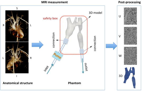
Figure 1: Schematic diagram of the phantom measurement. Left: anatomical 3D structures of a heart and great vessels (with CoA) were segmented and reconstructed based on MRI images to obtain the geometry of the aorta. Middle: 4D-Flow MRI of 3D printed phantoms connected to a pump were performd for pre-interventional and post-interventional geometries. Right: 4D-Flow MRI yields three components (U, V, W) of the instantaneous flow velocity at each voxel.

2.2 Numerical Modeling

The CFD simulations in this study were performed using the LBM, which is based on the kinetic theory, particularly the Boltzmann equation which describes the movements of fluid particles [23, 24, 25, 41]. For simulations, the space and time are discretized into finite nodes and time steps. Starting from an initial state, the configuration of the fluid particles at each time step evolves in two sub-steps, streaming and collision. During streaming, fluid particles at a node move to the neighbouring nodes along specified discrete directions as defined by the lattice. The streamed particles at a node collide with each other and change their velocity distribution functions [42]. For 3D flows, the most popular lattice is the D3Q19, which is used in this work.

Different operators, such as the single-relaxation time BGK [43] and the multi-relaxation-time (MRT) operators [44], can be used to approximate the particle collision. We chose the MRT operator due to its better numerical stability. The governing equation for the LBM with MRT operator reads

$$f_{i}\left(\mathbf{x}+\mathbf{e}_{i}\Delta t,t+\Delta t\right)-f_{i}(\mathbf{x},t)=\Lambda_{ij}(f_{j}^{eq}(\mathbf{x},t)-f_{j}(\mathbf{x},t)),$$ (1)

in which $f_{i}$ is the particle velocity distribution function along the $i$th direction; $\mathbf{x}$ and $t$ are the spatial coordinate and time respectively; $\Delta t$ is time step; $\mathbf{e}_{i}$ is the discrete velocity of the lattice along the $i$th direction. The right-hand side of Eq. (1) represents the collision process in momentum space. $\Lambda_{ij}=\mathbf{M}^{-1}\mathbf{S}\mathbf{M}$; $\mathbf{M}$ is a given transformation matrix for the lattice; $\mathbf{S}$ is a diagonal matrix. Macroscopic parameters, such as the fluid density, pressure and velocity, are moments of $f_{i}$.

The left-hand side and right-hand side of Eq. (1) represent the streaming and the collision processes respectively. The simplicity of this equation implies that the LBM is readily parallelizable as the non-local streaming is linear while the non-linear collision is local [23, 24, 25]. Thus, the LBM is increasingly used for turbulence modeling, especially DNS with high performance modern computers. Additionally, due to its particle feature, even with a simple Cartesian grid the LBM can resolve flow with complex geometry, such as the patient-specific aortas considered in this study.

The LBM based DNS and LES were investigated in this study, based on the open-source library Palabos [45]. DNS resolves the flow at all scales without empirical model, thus is regarded as a kind of numerical experiment. As mentioned before, the calculation cost of DNS is very high especially for flows with large Reynolds number [46, 27]. Alternatively, LES explicitly solves large eddy current and implicitly calculates small eddies by using a sub-grid scale (SGS) model, thus balancing accuracy and computational cost. The Smagorinsky SGS model [47] was incorporated into the LBM in this study.

For all simulations, the inlet velocity with Poiseuille profile was specified at the ascending aorta. The flow rates were given based on MRI measurements and can be found in the following sections. Outlet boundary condition with a reference pressure was applied to the descending aorta. The curved aortic wall was assumed to be no-slip and treated with an extrapolation scheme [48].

3 Validation and Comparison

3.1 Phantom Experiments

The two phantoms filled with water were used in the MRI experiments and compared to CFD simulations of the same geometries. The main branch blood vessels were closed, to reduce their influence. Inlet and outlet of the geometries were extended artificially for the connection of the water pipe. Water is incompressible and Newtonian. Its density and kinematic viscosity are 1.0 kg/m³ and 1.0 $\times 10^{-6}\text{m}^{2}\text{/s}$, respectively. The averaged velocity at the inlet is 0.1 m/s. Different spatial resolutions were considered for every single case. After mesh independence tests, 12.30 million (DNS) and 3.45 million (LES) lattice nodes were selected for the pre-interventional geometry and 5.12 million (DNS) and 1.25 million (LES) lattice nodes for the post-interventional one.

Due to the complex geometry, e.g. multiple plane curvatures and branches, blood flow in the patient-specific aorta is unsteady and complicated. Instantaneous velocity contours on a sagittal plane and a coronal plane in the pre-interventional geometry are given in Fig. 2. Due to the relatively low temporal resolution of 4D flow MRI, here only results from DNS and LES are presented. It can be seen that the flow therein is turbulent. Because of the local narrowing in the stenosis, flow is accelerated in the pre-interventional geometry and the local Reynolds number on the stenosis plane is more than 2500. Jet flow, which leads to high blood pressure and high wall shear stress (WSS), is observed. DNS provides more flow details due to higher spatial resolution.

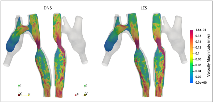
Figure 2: Instantaneous velocity contours on a sagittal plane and a coronal plane in the pre-interventional geometry of an aorta of a patient with CoA simulated by CFD. Left: DNS; right: LES.

As the flow is unsteady, temporal averaging was performed for both CFD and MRI results and the following comparison is based on the time-averaged flow fields. The main flow features can be found in Fig. 3. The visualization of 3D streamlines and velocity vectors on the sagittal plane (insets) shows the complexity of the flow within the patient’s aorta, especially where the stenosis occurs. Again, jet flow and recirculation are observed in the pre-interventional geometry in the streamlines and highlighted in the zoomed-in insets. Helical streamlines can also be found in all cases. For the MRI results, some streamlines start from the vessel wall as no-slip boundary condition is not guaranteed in MRI data. Nevertheless, all methods, including DNS, LES and MRI, resolved the main flow features. Moreover, as the aorta is deformed and flattened after stent implantation, the flow resistance in the post-interventional geometry is reduced. The pressure drop is reduced from 790 Pa (DNS) and 778 Pa (LES) to 9 Pa (DNS) and 8 Pa (LES), respectively. Those results indicate that stent implantation restored the aortic flow effectively.

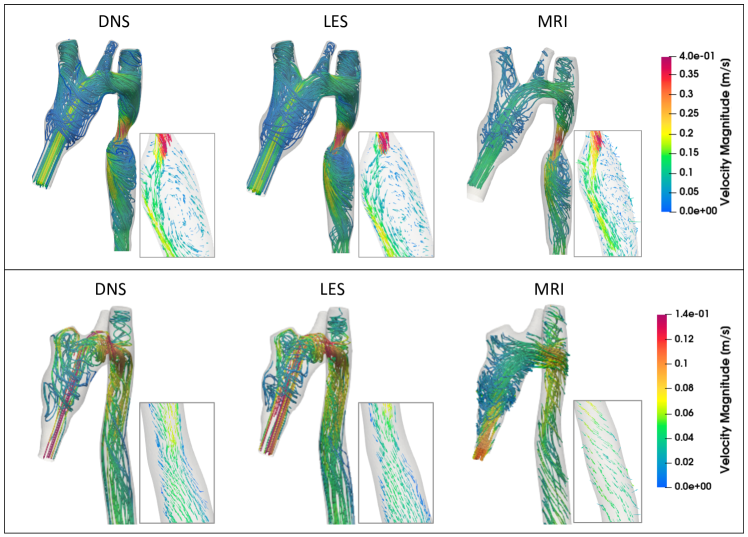
Figure 3: Streamlines of the flow computed with CFD simulations of the aorta compared to MRI measurements of the flow in the 3D-printed phantoms. The time-averaged flow is shown. The insets show the velocity vectors on the sagittal planes. Top: pre-interventional geometry; bottom: post-interventional geometry.

Figure 4 presents quantitative comparison of mean velocity magnitude on six specified cross-sectional planes. These six planes, as shown in the left panel of Fig. 4, represent the ascending, arch, pre-stenosis, on-stenosis, post-stenosis and descending of the aorta respectively. The mean velocity magnitude was calculated according to $\sum_{i=1}^{N}\sqrt{U_{i}^{2}+V_{i}^{2}+W_{i}^{2}}$ $/N$, with $N$ the number of points on a cross plane. It can be seen from the right panel of Fig. 4 that the MRI results are a little larger than the numerical ones on planes Pre 2, Pre 3 and Pre 5. Using MRI results as reference, the relative deviations for LES and DNS are $4-28\%$ and $7-27\%$ respectively. Largest deviation can be found on Pre 5, mainly due to the difficulty for the MRI measurement induced by the recirculation after the stenosis. On Pre 4, MRI data is between the DNS ($-4\%$) and LES ($7\%$) ones. For the post-interventional geometry, CFD results agree with the experimental data well on all planes, with relative derivations less than 10$\%$.

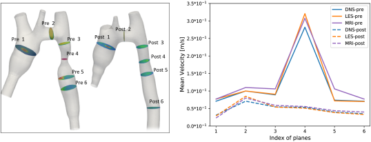
Figure 4: Comparison of mean velocity magnitude on specified planes for the pre-interventional and post-interventional aorta geometry. Left: six specified cross planes, including ascending, arch, pre-stenosis, on-stenosis, post-stenosis and descending of aorta. Right: The time-averaged mean velocities from 4D flow MRI and the CFD simulations.

Velocity contours on those specified planes, in pre-interventional and post-interventional geometries, are given in Figs. 5 and 6 respectively. Generally, flow patterns are qualitatively well-matched among LES, DNS and MRI for both geometries. Both LES and DNS provide more details and smoother fields due to higher spatial resolution compared with MRI. Discrepancy between the CFD results and MRI one is observed on Pre 4 and 5. We believe this is because of the complexity induced by the jet flow and recirculation after the stenosis, which is visualized in Figs. 2 and 3. Nevertheless, the results from LES agree very well with those from DNS on all specified planes.

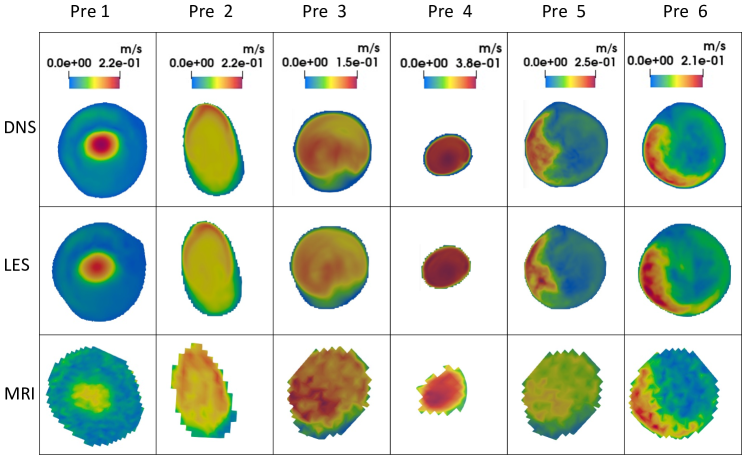
Figure 5: Flows in pre-interventional aorta. Velocity magnitude distributions were compared among CFD simulations and 4D Flow MRI on six planes as shown in Fig. 4. Time-averaged results.

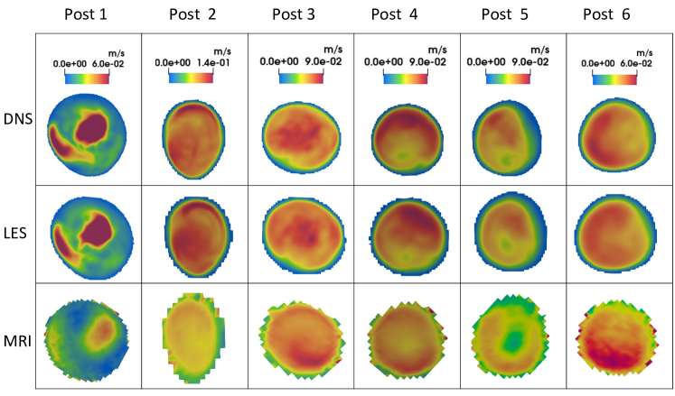
Figure 6: Flows in post-interventional aorta. Velocity magnitude distributions were compared among CFD simulations and 4D Flow MRI on six planes as shown in Fig. 4. Time-averaged results.

Velocities along the centerlines of the pre-interventional and post-interventional geometries were also compared. The centerline was extracted using the VMTK extension for 3D Slicer [49]. Since velocity in the pre-interventional geometry changes more acutely because of the stenosis, here only the results for pre-interventional geometry are presented. Discrete points along the centerline, starting from the ascending aorta after the artificial extension, are considered and can be found in the left panel of Fig. 7. Velocity components and magnitude are given in the right panel. It can be seen that velocity components change sharply in the stenosis region which leads to a peak in the profiles of velocity magnitudes. Results from LES, DNS, and MRI agree with each other in most region of the aorta, except the coarctation. Similarly to Fig. 5, discrepancy mainly happens in the MRI result around the stenosis, while good agreement between DNS and LES is always achieved.

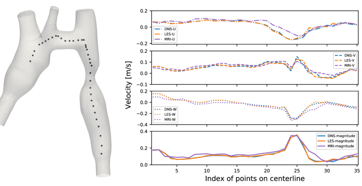
Figure 7: Comparison of flow velocity along the centerline of the pre-interventional aorta. Left: locations of the points starting from the ascending aorta. Right: from top to bottom, velocity components and magnitude. Time-averaged results.

Based on the above comparisons, it can be concluded that CFD (LES and DNS) results agree with the data from 4D-Flow MRI. More information, such as pressure drop and WSS can be easily generated from the CFD results. Since LES needs less computational resource but provides acceptable accuracy, we conclude that LES is capable in resolving aortic flow and adopt it for the following research.

3.2 In vivo Validation

To further validate the numerical modeling, we also used in vivo measurements in addition to the phantom study. The patient-specific aortic flow was compared between LES and flow MRI. Considering the long measurement duration needed by 4D-Flow MRI [50], 2D flow MRI was used for the in vivo scans. Velocities, thus flow rates, on specified planes perpendicular to the main flow direction were measured with 2D phase-contrast flow MRI. The experimentally obtained flow rate on a plane in the acceding aorta is shown in the left panel of Fig. 8. The two time instants, $t_{1}$ and $t_{2}$ during systole, were considered and their flow rates were used as inlet boundary condition for the LES simulations. The experimentally recorded velocity distributions in the descending aorta at these two instants were used for comparison.

In numerical simulations, the aortic geometry was segmented based on the MRI slices. We didn’t consider the deformation of the aorta, or fluid-solid interaction, and assumed that the wall was not moving. A parabolic velocity profile based on the experimentally recorded flow rate was specified as inlet. The opening in the descending aorta was defined as outlet with a reference pressure. Since the vessel branches were open in this test, the difference of flow rates between the inlet and outlet were assigned to the branches according to their cross areas [29, 51].

The time-averaged flow fields are given in the right panel of Fig. 8. At $t_{1}$ (the instant with peak flow rate), the through-plane component of mean velocity from LES is 0.69 m/s, with relative deviation 8$\%$ in reference to the MRI result, 0.75 m/s. Similarly, at $t_{2}$, the through-plane component of mean velocities are 0.55 m/s (LES) and 0.49 m/s (MRI). Thus, good agreement between LES and MRI was achieved also in vivo. Moreover, LES with proper boundary condition could provide more flow details due to higher spatial resolution, as shown in both in vivo and phantom tests.

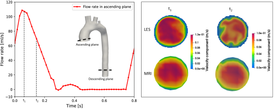
Figure 8: Comparison of in vivo aortic flow between LES and 2D flow MRI. Left: the experimentally recorded flow rate crossing the ascending plane; locations of the specified ascending plane and descending plane are given in the inset. Right: he through-plane component of velocity distributions on the descending plane at two different time instants during the cardiac cycle.

4 Application for Stent Selection

The main motivation for silico stent implantation is to help clinicians to evaluate the surgical plans based on predicted results and to be able to select an optimal stent already before surgery. A fast virtual stenting approach proposed by Neugebauer et al. [11] was implemented in this work to generate virtually deformed geometries. Several parameters, such as the aorta bending resistance, aorta stiffness, stent stiffness, stent position and diameter were considered in this approach to represent the interaction between aorta and stent. The deformed geometry deformation was then obtained based on the deformed centerline and deformed surface vertices. The original pre-interventional geometry and its deformed versions can be found in the left panel of Fig. 9. The deformed geometries were exported as STL files, which were remeshed and further imported into the CFD solver for flow simulation. It should be noted that in this study the physician chose a stent with diameter 12 mm independently and without input from the in slicio model. We compared the virtually deformed geometry based on this stent with the post-interventional one reconstructed from MRI images in the right panel of Fig. 9. Centerlines for both geometries were obtained and the distance ( $\leq 1.60$ mm) between two centerlines is presented. Similarly, the spatial dependent diameters are also given, with deviation less than 0.65 mm. It can be concluded that the virtually deformed geometry agrees with the clinically deformed one quantitatively.

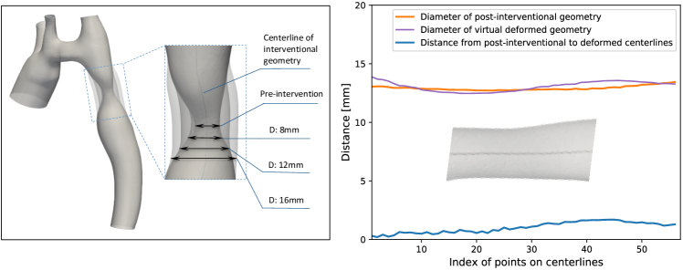
Figure 9: Virtual stent implantation and validation of deformation. Left: pre-interventional geometry, virtually deformed geometries with stent diameter 8 mm, 12 mm, and 16 mm respectively. Right: validation of virtual stent implantation, with inset showing the realistic post-interventional geometry.

The above validated LES was used to resolve the flows in the pre-interventional geometry and the virtually deformed ones. We used the same boundary conditions as mentioned in subsection 3.2, with flow rate 13.2 ml/s at the inlet. The numerically obtained results are presented in Figs. 10-11. The color coded streamlines in Fig. 10 show that a stent with diameter 8 mm is inadequate to reduce the stenosis and jet flow with a large local flow still can be observed in the narrowing region. For stent diameter 12 mm or 16 mm, the jet flow disappears, with substantially reduced maximum velocity compared to the pre-interventional geometry. The WSS distributions are given in Fig. 11. WSS describes the mechanical force generated by blood flow on the vessel wall, thus plays an important role in chronic adaption and remodelling [52]. It is defined as $\tau_{y=0}=\mu\frac{\partial u}{\partial y}\mid_{y=0}$, where $\mu$ is the dynamic viscosity of the flow, $u$ is the flow velocity along the wall and $y$ is the height above the wall. As shown in Fig. 11, high WSS is observed in the stenosis region in the pre-interventional geometry and the deformed one with stent diameter 8 mm. After the stenosis, high WSS is also found in a part of the descending aorta due to the impact of high-speed jet flow (see Fig. 10 for reference). A stent with diameter 16 mm enlarges the stenosis most and therefor leads to the smallest WSS in the same region. However, as this stent is larger than the size of the aorta, it also leads to a relatively large WSS before the stent, compared to the case with stent diameter of 12 mm.

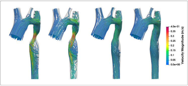
Figure 10: Streamlines in the pre-interventional and virtually deformed aortas. Time-averaged results. From left to right: pre-interventional geometry, virtually deformed geometries with stent diameter 8 mm, 12 mm, and 16 mm respectively.

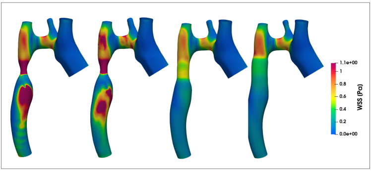
Figure 11: WSS on the pre-interventional and virtually deformed walls. Time-averaged results. From left to right: pre-interventional geometry, virtually deformed geometries with stent diameter 8 mm, 12 mm, and 16 mm respectively.

To quantitatively compare the four cases with different stent diameter, the pressure drop and maximum WSS are given in Fig. 12. It can be seen that the pressure drop is 119 Pa in the pre-surgical geometry, and is reduced to 34 Pa and 28 Pa in the geometry with stent diameter 12 mm and 16 mm respectively. For the maximum WSS on the aortic wall, the geometry with stent diameter 12 mm provides the smallest value, 1.07 Pa. It is understandable that a larger diameter stent results in less flow resistance thus smaller pressure drop, assuming that the aortic wall is always deformable. On the other hand, size of the aorta wall and its nonlinear response to possible strain should also be considered. If a stent is too large for the aorta, it is conceivable that in addition to flow there will be external mechanical force from the stent acting on the aortic wall. Thus a stent with diameter 12 mm should be the optimal solution for the current patient-specific aorta, which agrees with the physicians’ independent choice in this case.

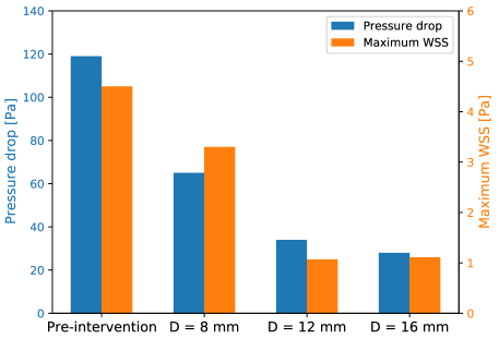
Figure 12: Quantitative comparison of pressure drop and maximum WSS in the aortas before and after deformation.

5 Discussion and Conclusion

Image-based in silico stent implantation [7, 8, 9, 11] and CFD [5, 6] together provide a new framework for stent planning and interventional procedure evaluation. Besides a protocol for virtual geometry deformation, a CFD method is needed to accurately resolve the flows in the aortic geometries. However, blood flow in patient-specific aorta is complicated [14, 15]. Laminar flow, turbulent flow and transition between them may coexist spatiotemporally. In our study, we firstly evaluated the accuracy of LES to predict such complicated flow. Two CFD methods, the LBM based LES and DNS, in cooperation with flow MRI, were considered. Both phantom and in vivo validations show that the LBM based LES, which keeps a balance between numerical accuracy and computational requirement, is a reasonable choice for resolving aortic flow. The validated LES was then used to predict the flows in virtually deformed geometries with different stent diameters. By comparing the flow fields, pressure drop, and maximum WSS, it was found that the optimal stent was the one with diameter 12 mm, which agrees with the physicians’ independent choice.

To restore blood flow, in addition to numerical methods, accurate geometry and boundary conditions are also important. Based on MRI scans, aortic geometry can be segmented and reconstructed from high-quality image slices [53, 54, 9]. Furthermore, flow MRI is used for visualization and quantification of aortic flow. 2D flow MRI with through-plane velocity encoding is usually performed in clinical applications [50, 55, 56]. But the 2D flow measurement is affected by the selection of the cross-sectional plane. 4D flow MRI, alternatively, is able to obtain time-dependent 3D blood flow, which is resolved in all three dimensions of space and the dimension of time during the cardiac cycle. It can used for the estimation of the flow pathways and the WSS. But 4D flow imaging takes a significant amount of time, which prevents wide clinical application. Thus for patient-specific in silico stent implantation, MRI and LES need to work together and both are indispensable. Particularly, MRI provides data for geometry and boundary conditions, while LES predicts aortic flows for further evaluation.

In this work, we validated the LBM based LES with both phantom and in vivo experiments, and provided a realistic example of the in silico stent implantation. There are still many improvements possible which could be considered in the future. Firstly, the aortic flow is unsteady, but we didn’t consider time dependent boundary condition in our simulations. We argue that current boundary conditions are enough for us to compare different methods and provide results for stent evaluation. By modeling the realistic cardiac cycle, one may get more instantaneous flow information at the cost of longer computation time. Secondly, we assigned the flow rates to the vessel branches according to their cross areas. An alternative is the Windkessel model which considers resistance and capacitance of the vessel network. Thirdly, we used a fast geometric method to mimic the complex interaction between the aortic wall and the stent. Ideally, one would take into account the mechanical properties of the aortic wall and the stent, and model their interaction using finite element method. Unfortunately it is still a big challenge to get accurate orthotropic properties of the fiber reinforced aortic wall and to model the contact problem numerically. Thus a simplified geometric method is a reasonable start. Finally, this methodology could also be extended to other stenosis, such as cerebral artery stenosis.

Conflict of interest

The authors have no conflict to disclose.

Ethics Declarations

This article does not describe studies with human or animal subjects. The anonymous images used in this article were obtained from a clinical database. Informed consent of the patients that permits research use of their data has been obtained beforehand.

References

- [1] Deniz Rafieianzab, Mohammad Amin Abazari, M. Soltani, and Mona Alimohammadi. The effect of coarctation degrees on wall shear stress indices. Scientific Reports, 11(1):1–13, 2021.
- [2] Julien I.E. Hoffman and Samuel Kaplan. The incidence of congenital heart disease. Journal of the American College of Cardiology, 39(12):1890–1900, 2002.
- [3] Mark D. Reller, Matthew J. Strickland, Tiffany Riehle-Colarusso, William T. Mahle, and Adolfo Correa. Prevalence of Congenital Heart Defects in Metropolitan Atlanta, 1998-2005. Journal of Pediatrics, 153(6):807–813, 2008.
- [4] Wail Alkashkari, Saad Albugami, and Ziyad M. Hijazi. Management of coarctation of the aorta in adult patients: State of the art. Korean Circulation Journal, 49(4):298–313, 2019.
- [5] Jingru Zhong, Yunling Long, Huagang Yan, Qianqian Meng, Jing Zhao, Ying Zhang, Xinjian Yang, and Haiyun Li. Fast Virtual Stenting with Active Contour Models in Intracranical Aneurysm. Scientific Reports, 6(February):1–9, 2016.
- [6] Philipp Berg, Sylvia Saalfeld, Gábor Janiga, Olivier Brina, Nicole M. Cancelliere, Paolo Machi, and Vitor M. Pereira. Virtual stenting of intracranial aneurysms: A pilot study for the prediction of treatment success based on hemodynamic simulations. International Journal of Artificial Organs, 41(11):698–705, 2018.
- [7] Aymeric Pionteck, Baptiste Pierrat, Sébastien Gorges, Jean-Noël Albertini, and Stéphane Avril. Evaluation and Verification of Fast Computational Simulations of Stent-Graft Deployment in Endovascular Aneurysmal Repair. Frontiers in Medical Technology, 3:704806, 2021.
- [8] Duanduan Chen, Jianyong Wei, Yiming Deng, Huanming Xu, Zhenfeng Li, Haoye Meng, Xiaofeng Han, Yonghao Wang, Jia Wan, Tianyi Yan, Jiang Xiong, and Xiaoying Tang. Virtual stenting with simplex mesh and mechanical contact analysis for real-time planning of thoracic endovascular aortic repair. Theranostics, 8(20):5758–5771, 2018.
- [9] Xiaoxin Kan, Tao Ma, Zhihui Dong, and Xiao Yun Xu. Patient-Specific Virtual Stent-Graft Deployment for Type B Aortic Dissection: A Pilot Study of the Impact of Stent-Graft Length. Frontiers in Physiology, 12(July), 2021.
- [10] R. McCloy and R. Stone. Science, medicine, and the future: Virtual reality in surgery. BMJ, 323(7318):912–915, 2001.
- [11] Mathias Neugebauer, Martin Glöckler, Leonid Goubergrits, Marcus Kelm, Titus Kuehne, and Anja Hennemuth. Interactive virtual stent planning for the treatment of coarctation of the aorta. International Journal of Computer Assisted Radiology and Surgery, 11(1):133–144, 2016.
- [12] T. J. Pedley. The Fluid Mechanics of Large Blood Vessels. Cambridge Monographs on Mechanics. Cambridge University Press, 1980.
- [13] T.R. Taha. An Introduction to Parallel Computational Fluid Dynamics, volume 6. 2005.
- [14] P. D. Stein and H. N. Sabbah. Turbulent blood flow in the ascending aorta of humans with normal and diseased aortic valves. Circulation Research, 39(1):58–65, 1976.
- [15] David N. Ku. Blood flow in arteries. Annual Review of Fluid Mechanics, 29:399–434, 1997.
- [16] A. D. Caballero and S. Laín. A Review on Computational Fluid Dynamics Modelling in Human Thoracic Aorta. Cardiovascular Engineering and Technology, 4(2):103–130, 2013.
- [17] F. P.P. Tan, A. Borghi, R. H. Mohiaddin, N. B. Wood, S. Thom, and X. Y. Xu. Analysis of flow patterns in a patient-specific thoracic aortic aneurysm model. Computers and Structures, 87(11-12):680–690, 2009.
- [18] Zhuo Cheng, Celia Riga, Joyce Chan, Mohammad Hamady, Nigel B. Wood, Nicholas J.W. Cheshire, Yun Xu, and Richard G.J. Gibbs. Initial findings and potential applicability of computational simulation of the aorta in acute type B dissection. Journal of Vascular Surgery, 57(2 SUPPL.):35S–43S, 2013.
- [19] Zhuo Cheng, Nigel B. Wood, Richard G.J. Gibbs, and Xiao Y. Xu. Geometric and Flow Features of Type B Aortic Dissection: Initial Findings and Comparison of Medically Treated and Stented Cases. Annals of Biomedical Engineering, 43(1):177–189, 2015.
- [20] C. A. Kousera, N. B. Wood, W. A. Seed, R. Torii, D. O’Regan, and X. Y. Xu. A Numerical Study of Aortic Flow Stability and Comparison With In Vivo Flow Measurements. Journal of Biomechanical Engineering, 135(1), 12 2012. 011003.
- [21] Shohei Miyazaki, Keiichi Itatani, Toyoki Furusawa, Teruyasu Nishino, Masataka Sugiyama, Yasuo Takehara, and Satoshi Yasukochi. Validation of numerical simulation methods in aortic arch using 4D Flow MRI. Heart and Vessels, 32(8):1032–1044, 2017.
- [22] Emily L. Manchester, Selene Pirola, Mohammad Yousuf Salmasi, Declan P. O’Regan, Thanos Athanasiou, and Xiao Yun Xu. Analysis of Turbulence Effects in a Patient-Specific Aorta with Aortic Valve Stenosis. Cardiovascular Engineering and Technology, 12(4):438–453, 2021.
- [23] Timm Krüger, Halim Kusumaatmaja, Alexandr Kuzmin, Orest Shardt, Goncalo Silva, and Erlend Magnus Viggen. The lattice boltzmann method. 2017.
- [24] Yaling He, Yong Wang, and Qing Li. Lattice boltzmann method: Theory and applications, 2009.
- [25] Shiyi Chen and Gary D Doolen. Lattice boltzmann method for fluid flows. Annual review of fluid mechanics, 30(1):329–364, 1998.
- [26] Hudong Chen, Satheesh Kandasamy, Steven Orszag, Rick Shock, Sauro Succi, and Victor Yakhot. Extended Boltzmann kinetic equation for turbulent flows. Science, 301(5633):633–636, 2003.
- [27] Yong Wang and S. Elghobashi. On locating the obstruction in the upper airway via numerical simulation. Respiratory Physiology and Neurobiology, 193(1):1–10, 2014.
- [28] Thomas Henn, Vincent Heuveline, Mathias J. Krause, and Sebastian Ritterbusch. Aortic coarctation simulation based on the lattice Boltzmann method: Benchmark results. In Lecture Notes in Computer Science (including subseries Lecture Notes in Artificial Intelligence and Lecture Notes in Bioinformatics), volume 7746 LNCS, pages 34–43, 2013.
- [29] Hanieh Mirzaee, Thomas Henn, Mathias J. Krause, Leonid Goubergrits, Christian Schumann, Mathias Neugebauer, Titus Kuehne, Tobias Preusser, and Anja Hennemuth. MRI-based computational hemodynamics in patients with aortic coarctation using the lattice Boltzmann methods: Clinical validation study. Journal of Magnetic Resonance Imaging, 45:139–146, 2017.
- [30] Michael Markl, Alex Frydrychowicz, Sebastian Kozerke, Mike Hope, and Oliver Wieben. 4D flow MRI. Journal of Magnetic Resonance Imaging, 36(5):1015–1036, 2012.
- [31] Graves MJ Prince MR McRobbie DW, Moore EA. MRI from Picture to Proton. Cambridge University Press, 2007.
- [32] Karl Landheer, Rolf F. Schulte, Michael S. Treacy, Kelley M. Swanberg, and Christoph Juchem. Theoretical description of modern 1h in vivo magnetic resonance spectroscopic pulse sequences. Journal of Magnetic Resonance Imaging, 51(4):1008–1029, 2020.
- [33] PR Moran. A flow velocity zeugmatographic interlace for nmr imaging in humans. Magnetic Resonance Imaging, 1(197–203), 1982.
- [34] M O’Donnell. Nmr blood flow using multiecho, phase contrast sequences. Medical Physics, 12(59–64), 1982.
- [35] Gilles Soulat, Patrick McCarthy, and Michael Markl. 4D Flow with MRI. Annual Review of Biomedical Engineering, 22:103–126, 2020.
- [36] Simone Saitta, Selene Pirola, Filippo Piatti, Emiliano Votta, Federico Lucherini, Francesca Pluchinotta, Mario Carminati, Massimo Lombardi, Christian Geppert, Federica Cuomo, Carlos Alberto Figueroa, Xiao Yun Xu, and Alberto Redaelli. Evaluation of 4D flow MRI-based non-invasive pressure assessment in aortic coarctations. Journal of Biomechanics, 94:13–21, 2019.
- [37] Paul A. Yushkevich, Joseph Piven, Heather Cody Hazlett, Rachel Gimpel Smith, Sean Ho, James C. Gee, and Guido Gerig. User-guided 3d active contour segmentation of anatomical structures: Significantly improved efficiency and reliability. NeuroImage, 31(3):1116–1128, 2006.
- [38] Singh K Schmidt R. Meshmixer: an interface for rapid mesh composition. In: ACM SIGGRAPH Talks; 2010; Los Angeles, NY, USA, 301, 2003.
- [39] Petter Dyverfeldt, Malenka Bissell, Alex J. Barker, Ann F. Bolger, Carl-Johan Carlhäll, Tino Ebbers, Christopher J. Francios, Alex Frydrychowicz, Julia Geiger, Daniel Giese, Michael D. Hope, Philip J. Kilner, Sebastian Kozerke, Saul Myerson, Stefan Neubauer, Oliver Wieben, and Michael Markl. 4D flow cardiovascular magnetic resonance consensus statement. Journal of Cardiovascular Magnetic Resonance, 17(1):1–19, 2015.
- [40] Wouter V Potters, Merih Cibis, Henk A Marquering, Ed VanBavel, Frank Gijsen, Jolanda J Wentzel, and Aart J Nederveen. 4D MRI-based wall shear stress quantification in the carotid bifurcation: a validation study in volunteers using computational fluid dynamics. Journal of Cardiovascular Magnetic Resonance, 2014.
- [41] Xiaoyi He and Lishi Luo. Theory of the lattice Boltzmann method: From the Boltzmann equation to the lattice Boltzmann equation. Physical Review E, 55(6):6811–6820, 1997.
- [42] Roberto Benzi, Sauro Succi, and Massimo Vergassola. The lattice Boltzmann equation: theory and application. Physics Reports, 222(3):145–197, 1992.
- [43] Yuehong Qian, Dominique D’Humières, and Pierre Lallemand. Lattice BGK models for Navier-Stokes equation. EPL, 17(6):479–484, 1992.
- [44] Dominique D’Humières, Irina Ginzburg, Manfred Krafczyk, Pierre Lallemand, and Lishi Luo. Multiple-relaxation-time lattice Boltzmann models in three dimensions. Philosophical Transactions of the Royal Society A: Mathematical, Physical and Engineering Sciences, 360(1792):437–451, 2002.
- [45] Jonas Latt, Orestis Malaspinas, Dimitrios Kontaxakis, Andrea Parmigiani, Daniel Lagrava, Federico Brogi, Mohamed Ben Belgacem, Yann Thorimbert, Sébastien Leclaire, Sha Li, Francesco Marson, Jonathan Lemus, Christos Kotsalos, Raphaël Conradin, Christophe Coreixas, Rémy Petkantchin, Franck Raynaud, Joël Beny, and Bastien Chopard. Palabos: Parallel lattice boltzmann solver. Computers & Mathematics with Applications, 81:334–350, 2021.
- [46] Parviz Moin and Krishnan Mahesh. Direct numerical simulation: A tool in turbulence research. Annual Review of Fluid Mechanics, 30(1):539–578, 1998.
- [47] J Smagorinsky. General circulation experiments with the primitive equations. part i, the basic experiment. Monthly Weather Review, 91(3):99–164, 1963.
- [48] Zhaoli Guo, Chuguang Zheng, and Baochang Shi. An extrapolation method for boundary conditions in lattice Boltzmann method. Physics of Fluids, 14(6):2007–2010, 2002.
- [49] Csaba Pinter, Andras Lasso, and Gabor Fichtinger. Polymorph segmentation representation for medical image computing. Computer Methods and Programs in Biomedicine, 171:19–26, 2019.
- [50] Zoran Stankovic, Bradley D Allen, Julio Garcia, and Kelly Jarvis. 4d flow imaging with mri. Cardiovascular diagnosis and therapy, 4(2):173–192, 2014.
- [51] S. Pirola, Z. Cheng, O. A. Jarral, D. P. O’Regan, J. R. Pepper, T. Athanasiou, and X. Y. Xu. On the choice of outlet boundary conditions for patient-specific analysis of aortic flow using computational fluid dynamics. Journal of Biomechanics, 60:15–21, 2017.
- [52] Jay D. Humphrey and Martin A. Schwartz. Vascular mechanobiology: Homeostasis, adaptation, and disease. Annual Review of Biomedical Engineering, 23:1–27, 2021.
- [53] Marwa M. A. Hadhoud, Mohamed I. Eladawy, Ahmed Farag, Franco M. Montevecchi, and Umberto Morbiducci. Left Ventricle Segmentation in Cardiac MRI Images. American Journal of Biomedical Engineering, 2(3):131–135, 2012.
- [54] MR Avendi, Arash Kheradvar, and Hamid Jafarkhani. Fully automatic segmentation of heart chambers in cardiac MRI using deep learning. Journal of Cardiovascular Magnetic Resonance, 18(S1):2–4, 2016.
- [55] Motonao Tanaka, Tsuguya Sakamoto, Shigeo Sugawara, Hiroyuki Nakajima, Takeyoshi Kameyama, Yoshiaki Katahira, Shigeo Ohtsuki, and Hiroshi Kanai. Spiral systolic blood flow in the ascending aorta and aortic arch analyzed by echo-dynamography. Journal of Cardiology, 56(1):97–110, 2010.
- [56] Andrew L. Wentland, Thomas M. Grist, and Oliver Wieben. Repeatability and Internal Consistency of Abdominal 2D and 4D Phase Contrast MR Flow Measurements. Academic Radiology, 20(6):699–704, 2013.