An Energy-dependent Electro-thermal Response Model of CUORE Cryogenic Calorimeter

Abstract

The Cryogenic Underground Observatory for Rare Events (CUORE) is the most sensitive experiment searching for neutrinoless double-beta decay ($0\nu\beta\beta$) in ${}^{130}\text{Te}$. CUORE uses a cryogenic array of 988 TeO₂ calorimeters operated at $\sim$10 mK with a total mass of 741 kg. To further increase the sensitivity, the detector response must be well understood. Here, we present a non-linear thermal model for the CUORE experiment on a detector-by-detector basis. We have examined both equilibrium and dynamic electro-thermal models of detectors by numerically fitting non-linear differential equations to the detector data of a subset of CUORE channels which are well characterized and representative of all channels. We demonstrate that the hot-electron effect and electric-field dependence of resistance in NTD-Ge thermistors alone are inadequate to describe our detectors’ energy dependent pulse shapes. We introduce an empirical second-order correction factor in the exponential temperature dependence of the thermistor, which produces excellent agreement with energy-dependent pulse shape data up to $6\text{\,}\mathrm{MeV}$. We also present a noise analysis using the fitted thermal parameters and show that the intrinsic thermal noise is negligible compared to the observed noise for our detectors.

1 Introduction

Neutrino-less double beta decay ($0\nu\beta\beta$) is a second-order nuclear process which, if observed, will violate the lepton number conservation in the Standard Model of particle physics. An observation of $0\nu\beta\beta$ decay would imply that at least one neutrino is Majorana in nature [1], place constraints on the neutrino masses [2], and will have fundamental implications for both neutrino and beyond Standard Model physics [3]. A constraint on the $0\nu\beta\beta$ decay half-life, even if the process is not directly observed, can still be converted into an inference on the effective neutrino mass[4]. The process also provides insight on how the imbalance between matter and anti-matter was created in early universe [5].

CUORE (Cryogenic Underground Observatory for Rare Events) is an ongoing tonne-scale experiment [6] searching for $0\nu\beta\beta$ in ¹³⁰Te. The detector contains a total 19 towers of $\text{TeO}_{2}$ crystals, each tower consisting of 52 $5\times 5\times 5\ $\text{\,}\mathrm{c}\mathrm{m}^{3}$$ cubic crystals. The low heat capacity of the crystals at cryogenic temperatures $\sim$10 mK provides measurable temperature changes for energy deposition events. The $\text{TeO}_{2}$ crystals are used as the source of double beta decays [7] coming from ${}^{130}\text{Te}$.

CUORE has placed a 90% Confidence Interval (CI) lower limit on the half life of ${}^{130}\text{Te}$ $0\nu\beta\beta$ as $2.2\text{\times}{10}^{25}\text{\,}\mathrm{y}\mathrm{r}$, a world-leading one regarding the process in ${}^{130}\text{Te}$ [8]. CUORE’s detection principle, the calorimetric approach, takes advantage of the fact that the energy for each detected radioactive event causes a sudden temperature increase in the $\text{TeO}_{2}$ crystal (absorber). CUORE uses Neutron Transmutation Doped (NTD) Germanium thermistors glued to the crystal to detect the subtle change in temperature [9, 10].

If the energy deposited is small enough, the response of the detector system can be solved exactly using a system of linear differential equations, with the signal pulse rise and decay time constants being a combination of different eigenvalues of the coefficient matrix. However, in CUORE there have been observed changes in pulse shape for events across a wide range of energies [11], from few tens of keV to $$6\text{\,}\mathrm{[}$]{\mega}$. We ascribe such changes to a different response of the whole system beyond the small-signal limit for high energy depositions. Since the region of interest (ROI) for CUORE is around[8] $Q_{\beta\beta}=$2527.518\pm 0.013\text{\,}\mathrm{keV}$$, which is in the middle of our energy range, it is imperative for us to better understand the behavior of the detector. Thus, we have developed an energy-dependent thermal model with physical parameters. Furthermore, because the energy interpreted for a generic calorimetric detectors depends on the pulse height, we find it advantageous to build a generic mathematical model framework for these calorimetric detectors. For CUORE, understanding the detector response is a prerequisite for pulse shape analysis (PSA). PSA enables effective filtering of energy-dependent pulse shapes, discriminates energy deposition based on particle type [12] and allows efficient triggering at low energies. With a model for the detector response, we can reproduce the pulses with higher fidelity and lower noise, potentially reducing timing jitter for each event. In addition, a model that describes the pulse shapes will be beneficial for machine learning algorithms for training and classification purposes.

The non-linear model is built on previous efforts that studied NTD-Ge thermistors in the linear (small-signal) regime. [13, 10, 14, 15, 16], and is able to predict the energy-dependence of the pulse shape. We adopt a combined model of both electrical field effect and hot electron effect to describe the electro-thermal property of the NTD-Ge semiconductor. In the thermal circuit, we also account for temperature-dependent heat capacities and thermal conductance. The simulated response is shown to be in close agreement with the observed signals across an extensive energy range if we include an additional second-order temperature correction to the NTD-Ge resistivity.

We conclude with a discussion on the noise response of the system based on the fitted model parameters. We observe excess noise in the CUORE measured noise power spectrum compared to the simulation. In our simulated noise model, a dominant contributor is the biasing resistor in the electrical circuit. Assuming additional $1/f$ and linear noise, the noise model can reproduce the continuous noise power spectra. However, because the CUORE electronics was designed to mitigate the $1/f$ noise, we are investigating the sources of the additional noise terms.

2 Electro-thermal Models

Thermal modeling for macrocalorimeters applies classical thermodynamics to the components of the calorimeters: the readout device (e.g. a thermistor) and its electrical circuit. Previous studies have extensively covered near-equilibrium calorimeters [17, 13, 18, 19, 20, 21, 22]. These studies provide comprehensive techniques of analyzing sensitive thermistors in small excursion from their equilibrium states, resulting in a handful of useful linear theories. However, the linear thermal models have a limitation that the response pulse shape is independent of event energy. We wish to find a non-linear model so that the pair annihilation peak, fully-contained high-energy $\gamma$ events (around $1$ to $2\text{\,}\mathrm{MeV}$) and $\alpha$ signals (around $6\text{\,}\mathrm{MeV}$) can be reproduced with the same set of parameters, similar to one of the previous studies [23] but in finer detail. We go to second order Taylor expansion near the equilibrium point of the detector to study the energy-dependent response of the calorimeter.

2.1 Electrical and Thermal Circuit

Each CUORE readout channel consists of a $\text{TeO}_{2}$ crystal, an NTD-Ge thermistor for temperature readout, a silicon-based heater for thermal gain stabilization, and several PTFE spacers for isolating the crystal from the heat-sink. The NTD-Ge thermistors have a dimension of $3.0\times 2.9\times 0.9\ $\text{\,}\mathrm{m}\mathrm{m}^{3}$$ ($L\times W\times H$) [24]. Figure 1 provides a qualitative description of the energy deposition process: the temperature of the crystal rises and so does the temperature of the thermistor system. The small heat capacity of the thermistor ensures that it closely follows the crystal temperature. In a few seconds, deposited energy flows out of the system through the thermal paths from the detector to the heat sink (the PTFE support and/or the NTD gold wires).

Figure 1: Simplified block diagram for CUORE thermal model. The crystal is modeled as a single object with heat capacity $C$ coupled to the heat-sink (with constant temperature $T_{0}$) through the PTFE support. When there is an energy deposition $E_{0}$ the heat flows through the PTFE support ($G_{1}$, $G_{2}$) and/or the NTD gold wires ($G_{4}$) and eventually to the heat-sink.

We start from a common readout circuit for thermal detectors as shown in Figure 2, where the bias resistor, together with a biasing voltage, determines the operational resistance of the detector. The bias resistor should be large compared to the thermistor so that the biasing circuit acts as a quasi-constant current source. In the case of extra energy deposition, the thermistor’s resistance decreases as its temperature increases. In this approximation, the current through the thermistor is held constant, and the thermistor’s self-heating power decreases along with the decrease in resistance, thus forming a negative thermal feedback that tends to stabilize the system. Realisitically, in such systems, the parasitic capacitance is also seen as a load, inserting possible instabilities at the frequency where the modulus of its impedance is equal to the thermistor impedance.

Figure 2: CUORE Detector electrical circuit. The two bias resistors before and after the NTD-Ge, labelled $R_{\rm{bol}}$, can be combined into one equivalent resistor $R_{\rm{bias}}$.

Additionally, the readout circuit, positioned outside the cryostat at 300K, holds some residual cable capacitance. The parasitic capacitance was measured and determined [25, 26] to be $C_{\textrm{p}}\approx$500\text{\,}\mathrm{pF}$$ between the detector cold stages at $10\text{\,}\mathrm{mK}$ and the front-end (FE) board. Therefore, we add the wire capacitance here in parallel with the thermistor in Figure 2. The corresponding electrical equation is:

$$C_{\textrm{p}}R_{\rm{bias}}\dot{V}_{\rm{bol}}(t)+\frac{V_{\rm{bol}}(t)}{R_{\rm{bol}}(t)}R_{\rm{bias}}+V_{\rm{bol}}(t)-V=0,$$ (2.1)

where $V$ is the constant voltage source bias. We note that the thermistor $R_{\rm{bol}}(V_{\rm{bol}}(t),T(t))$ is temperature and voltage dependent. This is our window to the thermal circuit.

Additionally, the output signal (NTD-Ge voltage $V_{\rm{bol}}$) is amplified and filtered through a 6-order Bessel filter. The transfer function of the Bessel filter is [26, 27]:

$$H(\sigma)=\frac{10395}{\sigma^{6}+21\sigma^{5}+210\sigma^{4}+1260\sigma^{3}+4725\sigma^{2}+10395\sigma+10395},$$ (2.2)

with $\sigma=2.703395061j\omega/(2\pi f_{c})$ and $f_{c}=$120\text{\,}\mathrm{H}\mathrm{z}$$. All our simulations producing $V_{\rm{bol}}$ are digitally amplified and filtered to match the true amplification and Bessel filter in the electronics readout chain.

The thermal power between materials of different temperatures usually takes the form of:

$$P_{i-j}=\int_{T_{j}}^{T_{i}}dT\,G_{i-j}(T)=g_{i-j}(T_{i}^{a_{i-j}}-T_{j}^{a_{i-j}}),$$ (2.3)

with the power flowing from node $i$ to node $j$ in the above equation. We use $G$ to denote the thermal conductance at a certain temperature, and $g$ to represent the thermal conductivity coefficient.

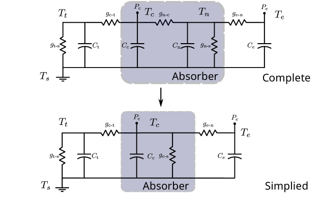
Figure 3: Thermal circuit for a single CUORE unit. The top diagram shows the components: PTFE support, the $\text{TeO}_{2}$ crystal, the NTD-Ge lattice, and the Ge electrons. The bottom diagram shows the crystal node simplified with the combination of the $\text{TeO}_{2}$ and NTD-Ge lattice.

Figure 3 shows the complete thermal circuit (top) and its simplified version (bottom) used in this work. The illustrated nodes from left to right are: PTFE support for the crystal, the $\text{TeO}_{2}$ crystal absorber, the NTD-Ge lattice glued to the crystal surface, and the electron system in the NTD-Ge lattice. There are gold wires connecting the NTD-Ge lattice to the copper frame (heat-sink) for NTD-Ge biasing and read-out, and thus we represent the conductivity term by its coefficient $g_{n-s}$. Similarly, $g_{n-c}$ represents the glue conductivity term connecting the NTD-Ge and the $\text{TeO}_{2}$ crystal, and $g_{e-n}$ represents the electron-phonon thermal coupling coefficient within the NTD-Ge sensor. We have neglected the thermal coupling from the Ge electrons directly to the heat-sink, since its effect is likely to be small compared to other thermal couplings, mainly the ones denoted by $g_{n-c}$, $g_{n-s}$, and $g_{e-n}$ [28, 27]. We further simplify the model by absorbing the NTD-Ge lattice node into the $\text{TeO}_{2}$ crystal node, as shown in the bottom part of Figure 3, effectively assuming that both nodes will always be at similar temperatures. We justify this by noting the tiny heat capacity of the NTD-Ge lattice, compared to that of the $\text{TeO}_{2}$ crystal, and the large thermal coupling between the Ge and the $\text{TeO}_{2}$ due to the glue. We have tabulated the estimated heat capacities for the calorimetric components in Table 1. Similarly, the effect of glue conductance is absorded in $g_{e-n}$, which now represents an effective conductance between the sensor electron system and the main absorber crystal.

Table 1: Table of estimated heat capacities of different components for CUORE crystals and NTD-Ges. The tiny capacity of the NTD-Ge lattice compared to the crystal and the electron system justifies its assimilation into the crystal node. The temperature dependence of the heat capacities are also revealed in the capacity matrix $C(T+\delta y)$.

Component Estimated Heat Capacity at $T=$10\text{\,}\mathrm{mK}$$ $[$\mathrm{J}\mathrm{/}\mathrm{K}$]$ Electrons [29, 30] $$1\text{\times}{10}^{-10}$\propto T$ NTD-Ge Lattice [31, 32] $$2.5\text{\times}{10}^{-14}$\propto T^{3}$ Crystal [33, 32] $$2.2\text{\times}{10}^{-9}$\propto T^{3}$ PTFE Support [34, 24] $$2.1\text{\times}{10}^{-8}$\propto T$

The combined node will have an additional thermal coupling to the heat-sink due to the gold wires bond to the Ge lattice. For book-keeping purposes, this conductivity coefficient is relabelled as $g_{c-s}$, and the electron-phonon coupling in the NTD-Ge lattice is relabelled as $g_{e-c}$. Apart from keeping the number of free parameters to a minimum, there is another reason for using three thermal nodes: in small signal limit, where the linear theory and solutions can be applied, the solution in the frequency domain with four poles and one zero is able to describe the CUORE pulses [35, 36]. Our choice of three thermal nodes plus one electrical read-out node fits comfortably in this picture.

2.2 Circuit Equations

We label the self-heating of the thermistor as $P_{e}$ and the power deposited on the crystal as $P_{c}$. Reading from the circuit, we have the following set of equations:

$$C_{e}\dot{T}_{e}=P_{e}-g_{e-c}\left(T^{a_{e-c}}_{e}-T^{a_{e-c}}_{c}\right),$$ (2.4)

$$C_{c}\dot{T}_{c}=P_{c} +g_{e-c}\left(T^{a_{e-c}}_{e}-T^{a_{e-c}}_{c}\right)$$ (2.5)

$$-g_{c-t}\left(T^{a_{c-t}}_{c}-T^{a_{c-t}}_{t}\right)$$

$$-g_{c-s}\left(T^{a_{c-s}}_{c}-T^{a_{c-s}}_{s}\right),$$

$$C_{t}\dot{T}_{t}= g_{c-t}\left(T^{a_{c-t}}_{c}-T^{a_{c-t}}_{t}\right)$$ (2.6)

$$-g_{t-s}\left(T^{a_{t-s}}_{t}-T^{a_{t-s}}_{s}\right).$$

If we expand eq. (2.1) near the equilibrium state (noted as "eq"), and denote:

$$R_{\rm{bol}} \to\overline{R}_{\rm{bol}}(eq)+\delta r_{\rm{bol}}(t),$$

$$V_{\rm{bol}} \to\overline{V}_{\rm{bol}}(eq)+\delta v_{\rm{bol}}(t),$$

we obtain a dynamic equation describing the changes in the terms of interest $R_{\rm{bol}}$ and $V_{\rm{bol}}$:

$$C_{\textrm{p}}R_{\rm{bias}}\dot{\delta v}_{\rm{bol}}+\frac{\delta v_{\rm{bol}}\overline{R}_{\rm{bol}}-\overline{V}_{\rm{bol}}\delta r_{\rm{bol}}}{\left(\overline{R}_{\rm{bol}}+\delta r_{\rm{bol}}\right)\overline{R}_{\rm{bol}}}R_{\rm{bias}}+\delta v_{\rm{bol}}=0.$$ (2.7)

We will present the thermistor’s dependence of $T_{e}$ and $V_{\rm{bol}}$ later in Section 2.3.

Regarding the thermal circuits eqs. (2.4) to (2.6), we follow a similar expansion around equilibrium to arrive at:

$$C\dot{\delta y}=\Delta P+\delta P_{i-j},$$ (2.8)

with

$$\delta P_{i-j}= g_{i-j}\left[(\overline{T}_{i}+\delta t_{i})^{a_{i-j}}-(\overline{T}_{j}+\delta t_{j})^{a_{i-j}}\right]$$ (2.9)

$$-g_{i-j}\left[\overline{T}_{i}^{a_{i-j}}-\overline{T}_{j}^{a_{i-j}}\right],$$

where $\delta t_{i}$ and $\delta t_{j}$ are the small changes in temperature from equilibrium $\overline{T}_{i}$, $\overline{T}_{j}$, and $\delta y$ represents a general vector of excursions from the equilibrium. The heat capacities $C$ are functions of temperature: $C=C(\overline{T}(eq)+\delta y)$. The $\Delta P$ term specifically denotes the electro-thermal feedback from the Joule heating of the NTD-Ge thermistor. This is the change in heating power of the thermistor when there is a change in electron temperature or voltage across the thermistor. Quantitatively:

$$\Delta P =\frac{(\overline{V}_{\rm{bol}}+(\delta v_{\rm{bol}}))^{2}}{\overline{R}_{\rm{bol}}+(\delta r_{\rm{bol}})}-\frac{\overline{V}_{\rm{bol}}^{2}}{\overline{R}_{\rm{bol}}}$$ (2.10)

$$=\frac{\overline{V}_{\rm{bol}}^{2}+2\overline{V}_{\rm{bol}}(\delta v_{\rm{bol}})+(\delta v_{\rm{bol}})^{2}}{\overline{R}_{\rm{bol}}+(\delta r_{\rm{bol}})}-\overline{P}.$$

In general we find a system of equations in the form:

$$C(\overline{T}+\delta y)\dot{\delta y}=f(\delta y)+x,$$ (2.11)

with

$$\delta y=\begin{bmatrix}\delta v_{\rm{bol}}\\ \delta t_{e}\\ \delta t_{c}\\ \delta t_{t}\end{bmatrix},C=\begin{bmatrix}C_{\rm{p}}\\ C_{e}(\overline{T_{e}}+\delta t_{e})\\ C_{c}(\overline{T_{c}}+\delta t_{c})\\ C_{t}(\overline{T_{t}}+\delta t_{t})\end{bmatrix}.$$ (2.12)

In eq. (2.11), $x$ is some additional injected power vector, such as the power injection due to some energy deposition in the crystal. The full form will be presented at the end of Section 2.3.

2.3 NTD-Ge Characteristics

NTD-Ge resistivity depends on its charge-carrier temperature ($T_{e}=\overline{T}_{e}+\delta t_{e}$) and applied voltage ($V_{\rm{bol}}=\overline{V}_{\rm{bol}}+\delta v_{\rm{bol}}$) across the chip. Since the temperature dependence of NTD-Ge is exponential, the behavior of the thermistor is expected to make a large contribution to the non-linearity we aim to study.

Starting from the Shklovskii-Efros law [13, 37] we obtain thermistor resistivity under zero bias voltage:

$$R(T_{e})=R_{0}\exp\left(\frac{T_{0}}{T_{e}}\right)^{\gamma}.$$ (2.13)

For low temperatures, $\gamma=0.5$ is the common value in literature [38]. It has also been observed that for extremely low temperatures (such as 10 mK), even injected power as low as $10^{-14}\ $\text{\,}\mathrm{W}$$ can induce non-ohmic behavior (i.e. deviation from eq. (2.13)) on the thermistor’s voltage-current (V-I) curve [32]. Usually such deviation at low temperature is attributed to electron-phonon thermal decoupling between the electrons and the NTD-Ge lattice [10] when the electrical field is small. That is, there exists a thermal resistance between the electrons and the NTD-Ge lattice, and their temperatures are related by:

$$P_{e}=I_{\rm{bol}}V_{\rm{bol}}=g_{e-n}(T_{e}^{a}-T_{n}^{a})=g_{e-c}(T_{e}^{a}-T_{c}^{a}).$$ (2.14)

We use the last equality when we combine the NTD-Ge lattice into the $\text{TeO}_{2}$ crystal node. Typical value for $a$ is around 5 to 6 [14]. However, studies have found that considering an additional term with E-field-induced hopping conduction often gives better agreement with data [15, 16]. We take the most widely accepted form derived by Hill [16, 39] for the modified resistivity:

$$R(V_{\rm{bol}},T_{e}) =R(0,T_{e})\exp\left(\frac{-eEL_{h}}{k_{B}T_{e}}\right)$$ (2.15)

$$=R_{0}\exp\left(\frac{T_{0}}{T_{e}}\right)^{0.5}\exp\left(\frac{-eV_{\rm{bol}}\lambda_{0}}{k_{B}T^{1.5}_{e}W}\right).$$

Here $L_{h}$ is the characteristic hopping length at a given temperature, which should, in theory scale with [40] $T^{-\gamma}=T^{-0.5}$. After changing the field strength $E$ into $V_{\rm{bol}}/W$ ($W$ being the effective thermistor width), we now describe the field correction term with a single unknown parameter $\lambda_{0}$.

Expanding eq. (2.15) near equilibrium but keeping the exponential, we obtain:

$$\overline{R}_{\rm{bol}}+\delta r_{\rm{bol}} =R_{0}\exp\left(\frac{T_{0}}{\overline{T}_{e}+\delta t_{e}}\right)^{\gamma}\exp\left[\frac{-C_{\lambda}\left(\overline{V}_{\rm{bol}}+\delta v_{\rm{bol}}\right)}{\left(\overline{T}_{e}+\delta t_{e}\right)^{\gamma+1}}\right]$$ (2.19)

$$=R_{0}\exp\left[\left(\frac{T_{0}}{\overline{T}_{e}}\right)^{\gamma}\left(1-\gamma\frac{\delta t_{e}}{\overline{T}_{e}}+...\right)\right]$$

$$\qquad\qquad\times\exp\left[-C_{\lambda}\frac{\overline{V}_{\rm{bol}}}{\overline{T}_{e}^{\gamma+1}}-C_{\lambda}\frac{\delta v_{\rm{bol}}}{\overline{T}_{e}^{\gamma+1}}+C_{\lambda}(\gamma+1)\frac{\delta t_{e}\overline{V}_{\rm{bol}}}{\overline{T}_{e}^{\gamma+2}}+...\right]$$

$$=\overline{R}_{\rm{bol}}\exp\left[-\eta\left(\frac{\delta t_{e}}{\overline{T}_{e}}\right)+C_{\lambda}(\gamma+1)\frac{\overline{V}_{\rm{bol}}}{\overline{T}_{e}^{\gamma+1}}\left(\frac{\delta t_{e}}{\overline{T}_{e}}\right)\right.$$

$$\left.\qquad\qquad\qquad-C_{\lambda}\frac{\overline{V}_{\rm{bol}}}{\overline{T}_{e}^{\gamma+1}}\left(\frac{\delta v_{\rm{bol}}}{\overline{V}_{\rm{bol}}}\right)+\mathcal{O}\left(\delta t_{e}^{2},\delta v_{\rm{bol}}^{2},\delta t_{e}\delta v_{\rm{bol}}\right)\right]$$

$$\equiv\overline{R}_{\rm{bol}}\exp(-\alpha),$$

where $\eta=\gamma\left(\frac{T_{0}}{T_{e}}\right)^{\gamma}$ is the temperature sensitivity, and $C_{\lambda}=e\lambda_{0}/k_{B}W$. Substituting the above results into eqs. (2.7) and (2.10), we have:

$$C_{\textrm{p}}R_{\rm{bias}}\dot{\delta v}_{\rm{bol}}+\delta v_{\rm{bol}}\frac{R_{\rm{bias}}}{\overline{R}_{\rm{bol}}}e^{\alpha} -\overline{V}_{\rm{bol}}\frac{R_{\rm{bias}}}{\overline{R}_{\rm{bol}}}\left(1-e^{\alpha}\right)+\delta v_{\rm{bol}}=0.$$

The thermal equation regarding the electrons becomes:

$$C_{e}\dot{\delta t}_{e}=\overline{P}_{e}\left(e^{\alpha}-1\right)+2\delta v_{\rm{bol}}\frac{\overline{V}_{\rm{bol}}}{\overline{R}_{\rm{bol}}}e^{\alpha}+\frac{\delta v_{\rm{bol}}^{2}}{\overline{R}_{\rm{bol}}}e^{\alpha}-\delta P_{e-c}.$$ (2.20)

We now summarize the system below (the bars are dropped for clarity):

$$C(T+\delta y)\dot{\delta y}\ =\begin{bmatrix}{\displaystyle-\delta v_{\rm{bol}}\left(\frac{e^{\alpha}}{R_{\rm{bol}}}+\frac{1}{R_{\rm{bias}}}\right)-\frac{V_{\rm{bol}}}{R_{\rm{bol}}}\left(e^{\alpha}-1\right)}\\[10.0pt] {\displaystyle P_{e}\left(e^{\alpha}-1\right)+\frac{2\delta v_{\rm{bol}}V_{\rm{bol}}}{R_{\rm{bol}}}e^{\alpha}+\frac{\delta v_{\rm{bol}}^{2}}{R_{\rm{bol}}}e^{\alpha}-\delta P_{e-c}}\\[10.0pt] {\displaystyle\delta P_{e-c}-\delta P_{c-t}-\delta P_{c-s}}\\[10.0pt] {\displaystyle\delta P_{c-t}-\delta P_{t-s}}\end{bmatrix}+x.$$ (2.21)

Specifically, $x=E_{0}\delta(t)$ is an event with energy $E_{0}$, with $\delta(t)$ being the Dirac delta. We use the SciPy solve_ivp [41] numerical solver that takes in an initial condition such that the crystal node starts with a change in temperature $t_{c}=E_{0}/C_{c}(\overline{T}_{c})$, with crystal heat capacity $C_{c}$ evaluated at equilibrium temperature $\overline{T}_{c}$.

Since our heat capacities are temperature dependent, and they are sensitive to the absolute temperature of the nodes, fitting these capacities is a method to infer the absolute temperature of the nodes at equilibrium. Linearization of the system around equilibrium can be simplified if we assume a constant capacity matrix at equilibrium $C(T)$ (which easily holds in our system for the equilibrium condition), and just taking the Jacobian of the right hand side $f(\delta y)$, we get:

(2.23)

Note $f(T)=0$ by the fact that at equilibrium the deviation is 0. We will refer to this linear system in the noise analysis in Section 5.

3 Equilibrium Model

In order to find an optimized operational resistance to achieve the best signal-to-noise (SNR) ratio and stability at a given temperature, CUORE incrementally tests the biasing voltage $V$ in eq. (2.1) and records the NTD-Ge voltage and current.

For details of how the V-I curves are taken and how errors are propagated, we refer to the work by Alfonso, et al [36]. The errors on the data are limited by the 10% accuracy of the bias resistor [35].

We use the equilibrium model to complement the dynamic model and to check the consistency of our fitted parameters. We used the bottom diagram of Figure 3 as the thermal circuit, and solve the temperature of each node in the thermal circuits eqs. (2.4) to (2.6) by setting the left hand side to 0 so that it is time independent. The electron temperature is then used to calculate the NTD-Ge resistance along with the NTD-Ge biasing voltage recorded in the V-I curves. The calculated resistances are fitted to the V-I curve resistances by minimizing the least squares between them.

During the CUORE optimization campaign, V-I curves at several temperatures (from $12\text{\,}\mathrm{mK}$ to $27\text{\,}\mathrm{mK}$) were acquired only for 78 of the 988 detectors, which were identified as representative channels for the whole array. Our analyses in the rest of the paper apply to these 78 channels. The NTD-Ge types in these towers cover all types used in CUORE (tower 8 — NTD 41C, tower 9 — NTD 39C, tower 10 — NTD 39D). As the NTD-Ge thermistors in the same tower are diced from the same wafer, we make the assumption that NTD-Ge parameters obtained from the same tower share common parameter distributions, and consequently they can be used on a tower basis to characterize the same type of NTD-Ge thermistors in other towers. We summarize the fit results by NTD batches in Table 2. All NTD batches are nominally irradiated to the same neutron fluence of about $3.4\text{\times}{10}^{18}\text{\,}\mathrm{n}\mathrm{/}\mathrm{c}\mathrm{m}^{2}$ at MIT Nuclear Research Laboratory, but the position with respect to the neutron beam and the number of irradiation passes are different. The errors in the table are standard deviations of the parameter spread in the same tower.

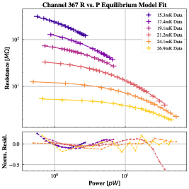
(a) Channel 367 from tower 8.

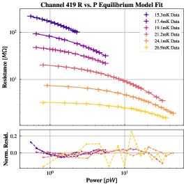
(b) Channel 419 from tower 9.

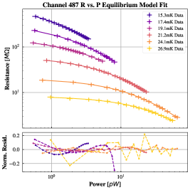
(c) Channel 487 from tower 10.

Figure 4: V-I fits for three sample channels from tower 8, 9, and 10 of CUORE. Each tower represents a different batch of produced NTD-Ge. Each V-I curve was taken at different heat-sink temperatures. The electron-phonon coupling within the NTD-Ge thermistor is much weaker than other couplings between the calorimeter components.

Table 2: Summary of NTD-Ge V-I curve fits by NTD-Ge batch.

$P_{\textrm{os}}\ [$\mathrm{W}$]$ $R_{0}\ [$\mathrm{\SIUnitSymbolOhm}$]$ $T_{0}\ [$\mathrm{K}$]$ $a_{e-c}$ $g_{e-c}\ [$\mathrm{W}\mathrm{/}\mathrm{K}^{a_{e-c}}$]$ $\lambda_{0}\ [$\mathrm{n}\mathrm{m}\cdot\mathrm{K}^{0.5}$]$ NTD batch $\left(7.70\pm 0.62\right)\times 10^{-13}$ $0.474\pm 0.035$ $7.04\pm 0.19$ $5.36\pm 0.13$ $0.0154\pm 0.0082$ $13.8\pm 2.6$ 39C $\left(7.8\pm 1.5\right)\times 10^{-13}$ $0.58\pm 0.15$ $7.58\pm 0.15$ $5.81\pm 0.42$ $0.11\pm 0.15$ $7.9\pm 7.6$ 39D $\left(6.90\pm 0.80\right)\times 10^{-13}$ $0.622\pm 0.053$ $6.78\pm 0.16$ $5.70\pm 0.18$ $0.042\pm 0.020$ $3.8\pm 4.3$ 41C

We have observed that for the electron-phonon coupling within the NTD-Ge thermistor, its thermal conductance G is much smaller than the thermal conductances for coupling between the $\text{TeO}_{2}$ crystal and the heat-sink, and general coupling between the PTFE support and the heat-sink. This observation implies that the V-I data alone could not determine the power law of thermal coupling beyond that of the electron-phonon coupling. The fitting is not sensitive to changes in initial values for coupling between the $\text{TeO}_{2}$ crystal and the heat-sink or the coupling between the PTFE support and the heat-sink. We plot the fits on sample channels in Figure 4.

We also note that the $T_{0}$ values, as appearing in eq. (2.13), are about one to two Kelvins higher than previously reported measurements [42], while the $R_{0}$ values are lower than previous characterizations. The $R_{0}$ parameter is highly anti-correlated with $T_{0}$ by the nature of the eq. (2.13), which should explain the fits’ underestimation. The electron-phonon coupling power law coefficient $a_{e-c}$, and $\lambda_{0}$ are close to expectation: $a_{e-c}$ values are between 5 and 6, while $\lambda_{0}$ parameters [16] are on the order of $10\text{\,}\mathrm{n}\mathrm{m}\cdot\mathrm{K}^{0.5}$.

4 Dynamic Model

The dynamic model aims to explain the energy dependence of calorimeter signal pulses. A linear system has a constant conductivity matrix $G(T)$ and a constant capacity matrix $C(T)$ in eq. (2.3), and thus it does not predict any change in pulse shape regardless of the input energy because eigenvalues of the these two matrices are fixed. This is not true for CUORE pulses, and we seek to model the detector response using eq. (2.21) for pulses up to the alpha region ($<6$ MeV) in this section.

We use the same model as we have verified using the V-I curves in Section 3. For a given base temperature and NTD working point, we group a set of 5 pulses with different energies together and perform a simultaneous fit on each group of 5 pulses to increase our model sensitivity towards energy dependence of the pulse shape. Each group includes energies ranging from $511\text{\,}\mathrm{keV}$ to $5407\text{\,}\mathrm{keV}$, which are chosen from the energy spectrum peaks of the dataset. We input these energies as the initial condition for the simulations, and fit by minimizing the squared difference between the raw pulses and simulations. We are also fitting the heat-sink temperature, assuming that the heat-sink temperatures for all of the pulses are close enough so that the five pulses can be described by the same heat-sink temperature. The model is tested on the same 78 channels as introduced in Section 3. Each channel has 40 "groups" of simultaneous fits. To correct for signal baseline drifts, we have added two corrections for each pulse: a linear correction parametrized by $V_{\rm{lin}}=m(t-b)$, where $m$ is the slope and $b$ is the intercept; and an exponential tail correction parametrized by $V_{\rm{exp}}=Ae^{-t/\tau}$, where $A$ is the initial amplitude at time 0 and $\tau$ is the characteristic decay time. The linear correction is often caused by thermal drifts of the detector or changes of the cryostat’s noise environment, especially vibration noises at low frequencies, whereas the exponential correction usually results from the decay of a previous event sufficiently close to the examined one. The fit results for key model parameters are listed in Table 3.

Table 3: Table of key parameter initial values used in the fit. If the parameter has an error estimation in the table, then a parameter is given a prior. The prior is assumed to be gaussian and given a boosted weighting of 100, as otherwise we find it hard for the priors to be effective in constraining the fit parameters. The parameter expectation values are confined by previous measurements [28, 27, 23, 11].

Parameter Name Symbol Unit Value Pulse Time $t_{\textrm{p}}$ $\mathrm{s}$ $3$ Parasitic Capacitance $c_{\textrm{p}}$ $\mathrm{pF}$ $500\pm 100$ Electron Heat Capacity [35, 24] $c_{e}$ $\mathrm{J}\mathrm{/}\mathrm{K}$ $8.6\text{\times}{10}^{-11}$ $\text{TeO}_{2}$ Crystal Heat Capacity $c_{c}$ $\mathrm{J}\mathrm{/}\mathrm{K}^{4}$ $(2.2\pm 0.2)\text{\times}{10}^{-3}$ PTFE Support Heat Capacity $c_{t}$ $\mathrm{J}\mathrm{/}\mathrm{K}^{2}$ $(2.1\pm 0.2)\text{\times}{10}^{-6}$ Electron-Phonon Thermal Conductivity $g_{e-c}$ $\mathrm{W}\mathrm{/}\mathrm{K}^{a_{e-c}}$ From Table 2 (NTD-dependent) Crystal-PTFE Thermal Conductivity $g_{c-t}$ $\mathrm{W}\mathrm{/}\mathrm{K}^{a_{c-tef}}$ $1\text{\times}{10}^{-8}$ PTFE-heat-sink Thermal Conductivity $g_{t-s}$ $\mathrm{W}\mathrm{/}\mathrm{K}^{a_{tef-s}}$ $1\text{\times}{10}^{-8}$ Electron-Phonon Conductivity Power Exponent $a_{e-c}$ N/A From Table 2 (NTD-dependent) Absorber-PTFE Conductivity Power Exponent $a_{c-t}$ N/A $1$ (Fixed) PTFE-hea-sink Conductivity Power Exponent $a_{t-s}$ N/A $1$ (Fixed) NTD-Ge Characteristic Temperature $T_{0}$ $\mathrm{K}$ From Table 2 (NTD-dependent) NTD-Ge Characteristic Hopping Length $\lambda_{0}$ $\mathrm{n}\mathrm{m}\cdot\mathrm{K}^{0.5}$ From Table 2 (NTD-dependent) Heat-sink Temperature $T_{\rm{base}}$ $\mathrm{K}$ $0.010\sim 0.015$

During the fitting process, we find that despite the use of simultaneous fit, the least square loss converges slowly if too many input parameters are provided. Therefore, we set the thermal coupling between the $\text{TeO}_{2}$ crystal and the heat-sink to zero, and have also fixed both power exponents of the coupling between the crystal and its PTFE support and the coupling between the PTFE support and the heat-sink to 1 so that the heat conductance becomes independent of temperature. Both changes have no noticeable effects on the fit results. The equivalent thermal circuit diagram is shown in figure Figure 5.

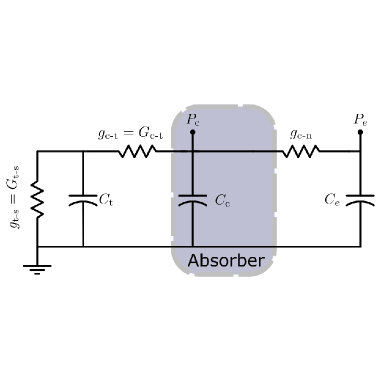
Figure 5: The thermal circuit used in the dynamic model. The direct coupling between the crystal and heat-sink has been removed because the fit is not sensitive to this parameter.

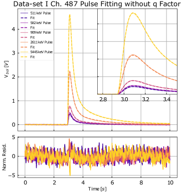
Figure 6: Grouped pulse fit for sample channel 487 for data-set I ($15.3\text{\,}\mathrm{mK}$). The residual normalized with the standard deviation of the first 2 seconds of the waveform is plotted at the bottom. The inset shows a zoomed portion of the peak.

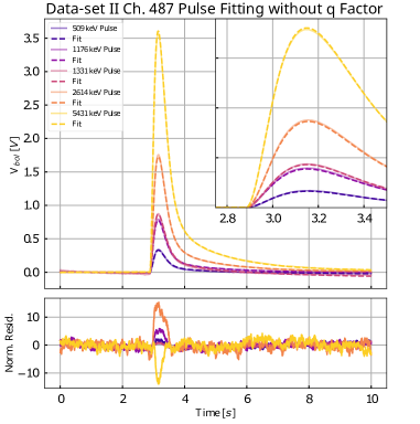
Figure 7: Grouped pulse fit for sample channel 487 for data-set II ($11.9\text{\,}\mathrm{mK}$). The normalized residuals are large near the peak of the signal pulses. This means the model pulse is over-shooting the peak in the highest energy, while the other pulses are underestimating the peak. The model without the $q$ factor cannot address this deviation.

Figure 6 (for data-set I, $15.3\text{\,}\mathrm{mK}$) and Figure 7 (for data-set II, $11.9\text{\,}\mathrm{mK}$) both show one of the sample group fits. To compare with the equilibrium model, we tabulate the mean and the standard deviation of key fit parameters in Table 4. We note that almost all key parameters from the V-I curve model are close to the fitting results from the dynamic model, suggesting that the dynamic model is consistent with the earlier equilibrium model.

Table 4: Principal fit parameters of the dynamic model, grouped by NTD-Ge batch. The Roman numeral subscript after $T_{s}$ denotes the data-set number. The parameter fit values for both data-sets are compatible with each other and thus combined.

$c_{\textrm{p}}\ [$\mathrm{pF}$]$ $g_{e-c}\ [$\mathrm{W}\mathrm{/}\mathrm{K}^{a_{e-c}}$]$ $a_{e-c}$ $T_{0}\ [$\mathrm{K}$]$ $\lambda_{0}\ [$\mathrm{n}\mathrm{m}\cdot\mathrm{K}^{0.5}$]$ $T_{s,I}\ [$\mathrm{mK}$]$ $T_{s,II}\ [$\mathrm{mK}$]$ NTD batch $511\pm 17$ $0.026\pm 0.002$ $5.07\pm 0.07$ $7.039\pm 0.009$ $12.3\pm 0.9$ $13.1\pm 0.8$ $12.2\pm 1.4$ 39C $501\pm 9$ $0.17\pm 0.02$ $5.52\pm 0.10$ $7.576\pm 0.004$ $8.6\pm 4.2$ $13.0\pm 0.9$ $11.3\pm 0.6$ 39D $514\pm 14$ $0.058\pm 0.002$ $5.34\pm 0.06$ $6.771\pm 0.007$ $2.0\pm 1.3$ $13.3\pm 0.4$ $11.3\pm 0.6$ 41C

Table 5: Principal fit parameters of the dynamic model with $q$ factor, grouped by NTD batch.

$c_{\textrm{p}}\ [$\mathrm{pF}$]$ $g_{e-c}\ [$\mathrm{W}\mathrm{/}\mathrm{K}^{a_{e-c}}$]$ $a_{e-c}$ $T_{0}\ [$\mathrm{K}$]$ $\lambda_{0}\ [$\mathrm{n}\mathrm{m}\cdot\mathrm{K}^{0.5}$]$ $q$ $T_{s,I}\ [$\mathrm{mK}$]$ $T_{s,II}\ [$\mathrm{mK}$]$ NTD batch $513\pm 18$ $0.026\pm 0.002$ $5.05\pm 0.07$ $7.039\pm 0.008$ $12.4\pm 0.9$ $-34\pm 15$ $12.8\pm 0.9$ $10.7\pm 1.2$ 39C $507\pm 10$ $0.17\pm 0.02$ $5.48\pm 0.10$ $7.577\pm 0.004$ $10.5\pm 3.8$ $-32\pm 11$ $12.7\pm 1.0$ $10.6\pm 1.2$ 39D $523\pm 15$ $0.059\pm 0.002$ $5.34\pm 0.06$ $6.770\pm 0.007$ $2.7\pm 1.4$ $-32\pm 10$ $13.2\pm 0.4$ $11.1\pm 0.7$ 41C

However, the residuals stray away from zero near the peak of the pulses. We find that introducing an empirical second-order correction term to the NTD-Ge resistivity expansion, defined in eq. (2.19), produces better fitting results. To test if the additional second-order correction can be explained by the standard law, i.e. eq. (2.15), we separate its expansion to the second order so that:

$$\alpha\to\alpha -\frac{3}{4}\eta\left(\frac{\delta t_{e}}{T_{e}}\right)^{2}+\frac{15}{8}C_{\lambda}\frac{V_{\rm{bol}}}{T_{e}^{1.5}}\left(\frac{\delta t_{e}}{T_{e}}\right)^{2}$$ (4.24)

$$-\frac{3}{2}C_{\lambda}\frac{V_{\rm{bol}}}{T_{e}^{1.5}}\left(\frac{\delta t_{e}}{T_{e}}\right)\left(\frac{\delta v_{\rm{bol}}}{V_{\rm{bol}}}\right)+q\left(\frac{\delta t_{e}}{T_{e}}\right)^{2}.$$

Our null hypothesis is that the additional $q$ factor is 0. Fit results on data-sets I and II with the inclusion of the $q$ factor have notably improved, as can be inferred from the comparison of the histograms of reduced $\chi^{2}$ figure-of-merit in Figure 8. Figure 9 showing the fitting of the same group of pulses as those in Figure 7 confirms this observation.

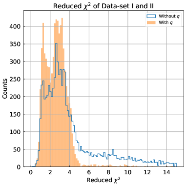
Figure 8: Comparison between the histograms of the reduced $\chi^{2}$ values for the simultaneous fits performed on data-sets I and II. The higher reduced $\chi^{2}$ peak in the "double-bump" feature corresponds to channels in the NTD batches 41C and 39C, which in general show a poorer quality of fit even without the $q$ factor.

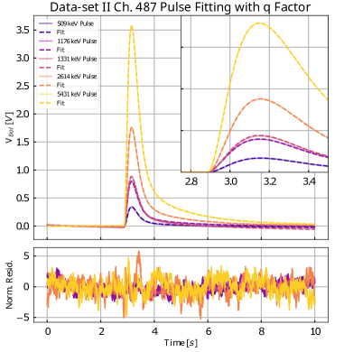
Figure 9: Grouped pulse fit for sample channel 487 for data-set II with $q$ factor. Cf. Figure 7. The normalized residuals for all the pulses are closer to being evenly distributed around 0.

The parameters in the modified dynamic model are summarized in Table 5, where we have applied a reduced $\chi^{2}$ cut of 5 in the fitting results for filtering out spurious pulses when calculating the statistics. Pulses with high reduced $\chi^{2}$ could be caused by unstable baseline or pileups. The cutoff is supposed to exclude these not well-fitted pulses so that the fit parameters are more credible.

As listed in the table, the $q$ factors have distributions not compatible with the null hypothesis and are negative. This result suggests possible unaccounted correction terms in the NTD-Ge characteristic function. It is not likely that such factor arises from subtleties in the thermal couplings between the crystal and the PTFE support or the heat-sink, as they affect the long pulse decay time constant. Since a negative $q$ factor means that the expansion $\alpha$ is more concave down, it could implie a larger $\gamma$ value in eq. (2.13). More experimental efforts are necessary in the future to determine the origin of this correction.

At the end of this section, by comparing to the equilibrium model results in Table 2, we note that most values we obtain in Table 5 are consistent. The heat-sink temperature fitting results have systematic deviations of around $\mathrm{-}\mathrm{1}$ to $-2.5\text{\,}\mathrm{mK}$. Another difference is that the power law exponents $a_{e-c}$ are universally lower in the dynamic model than in the equilibrium model. This implies that other thermal couplings with smaller power exponents may be present in the system.

5 Noise

Obtaining the physical parameters allows us to analyze major noise contributions from both thermal and electrical circuits. The numerical simulation can be carried out in the frequency domain. We begin by performing a Fourier transformation on the linear system eq. (2.3):

$$(i\omega C-G)Y(\omega)=X(\omega).$$ (5.1)

The right hand side of the equation represents the noise input, and with appropriate input vector the output vector $Y$ simulates the detector response.

There are two major kinds of noises: Thermal Fluctuation Noise (TFN) and Johnson noise from the readout circuit. Both have frequency-independent power spectra, but TFN has a stronger temperature dependency. We can use the TFN between charge carriers and NTD-Ge lattice as an example of incorporating TFN. The noise source features the following spectrum [13]:

$$p^{2}_{T-e-n}=4kT^{2}GF_{\textrm{link}},$$ (5.2)

where

$$F_{\textrm{link}}=\frac{(T_{e}/T_{n})^{\beta+2}+1}{2},$$ (5.3)

and where $\beta$ is the temperature dependence of $G$ and we note here that $P\sim gT^{\beta+1}$. For TFN between two nodes at equilibrium with each other, the link term $F_{\textrm{link}}=1$. In our system (radiative limit), the link term accounts for the temperature gradient at the two ends.

Then our input vector is:

$$X(\omega)=\begin{bmatrix}0\\ p_{T-e-c}\\ -p_{T-e-c}\\ 0\end{bmatrix}.$$ (5.4)

We note that an increase of power for the charge carriers in the context of noise indicates a decrease of power on the opposite side, and hence the minus sign before $p_{T-e-c}$. The absolute value of the output vector is the average noise power due to electron-phonon TFN.

To evaluate the contribution of the Johnson noise, there are two parts: the bias resistor and the thermistor. We refer to a similar study on transition-edge sensors (TES) for the derivation [18]. Noise from the bias resistor can be expressed as an external voltage source, as shown in Figure 10.

Figure 10: Equivalent Johnson noise generation circuits for the bias resistor $R_{\rm{bias}}$ and NTD-Ge thermistor $R_{\rm{bol}}$.

We emphasize that the physical dimension of the input $X$ is equivalent to $GY$ and is in $\mathrm{A}\mathrm{/}\sqrt{\mathrm{Hz}}$ for the electrical node, so we need to use the noise current (the voltage divided by resistance) instead of voltage:

$$i_{J-L}=\frac{e_{J-L}}{R_{\rm{bias}}}.$$ (5.5)

In general the linearized system takes care of the electro-thermal feedback through the matrix $G$, and thus the input is:

$$X(\omega)=\begin{bmatrix}i_{J-L}\\ 0\\ 0\\ 0\end{bmatrix}.$$ (5.6)

Regarding the Johnson noise for NTD-Ge, we refer to the right plot of Figure 10 for the noise circuit. The effective input on the electrical node is still current input, but this time there is an additional power correction $-\overline{I}_{b}v_{J-b}$ as the measured voltage includes the voltage across the thermistor (responsible for electro-thermal feedback) plus the voltage noise. The input vector is then:

$$X(\omega)=\begin{bmatrix}i_{J-b}\\ -\overline{I}_{b}v_{J-b}\\ 0\\ 0\end{bmatrix}.$$ (5.7)

Incorporating other thermal fluctuation noises, we find the noise input vector as the following:

$$X(\omega)=\begin{bmatrix}i_{J-L}+i_{J-b}\\ -\overline{I}_{b}v_{J-b}+p_{T-e-c}\\ -p_{T-e-c}+-p_{T-c-tef}\\ p_{T-c-tef}+p_{T-tef-s}\end{bmatrix}.$$ (5.8)

Figure 11a and Figure 11b show the total noise simulation along with the measured noise power spectrum (NPS) for both data-sets, before the amplifier gain but with the Bessel filter. The system noise floor is set by the digitizer ADC range and thus changes with different system gains for the two data-sets. To give a better sense of the noise level, we also include the NPS plot of channel 474 in Figure 11c, which is more representative of the CUORE channels. In Table 6, we have also listed the bias circuit settings and digitization system (i.e. the front-end board) data, such as the resistance of the NTD-Ge thermistor at the biasing point, the system gain, and total root-mean-square (RMS) voltage when there are no pulses for the sample channel. The sample channel is selected as the same one in Section 4. We can observe that the Johnson noise from the bias resistor is the major noise source. However, the considered total noise only account for approximately 1/10 of the measured NPS. The figures also show that the continuous power spectrum contains a $1/f$ component. This component cannot arise from the white Johnson noise alone because with the capacitance matrix in eq. (5.1), white noise input spectrum always outputs $1/f^{2}$ power spectrum. We thus add two extra input current noise terms:

$$i^{2}_{\rm{ext}}=C_{1}f+\frac{C_{2}}{f}.$$ (5.9)

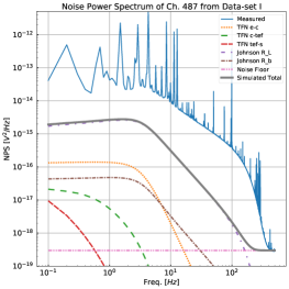
(a) Channel 487, data-set I.

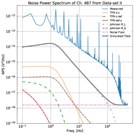
(b) Channel 487, data-set II.

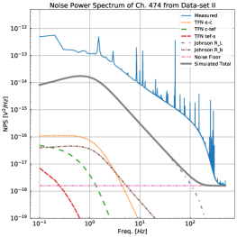
(c) Channel 474, data-set II.

Figure 11: Left and Middle: Simulated NPS for channel 487 overlaid with measured NPS from data-set I and II. Right: NPS for channel 474 from data-set II. We include this channel because it is more representative of an average CUORE channel. Spectra are divided by the gain of the amplification chain and multiplied with the Bessel filter transfer function.

Table 6: Bias circuit settings and digitization system data of channel 487 used in the NPS plots. The $V$ column lists the total biasing voltage of the electrical circuit in Figure 2. The gain column denotes the gain of the front-end amlification stage. The scaled baseline RMS is the raw baseline RMS scaled by the system gain.

$R_{\rm{bias}}(R_{\rm{L}})\ [$\mathrm{G\SIUnitSymbolOhm}$]$ $V\ [$\mathrm{V}$]$ $R_{\rm{bol}}\ [$\mathrm{M\SIUnitSymbolOhm}$]$ Raw Baseline RMS [$\mathrm{\SIUnitSymbolMicro V}$] Gain Scaled Baseline RMS [$\mathrm{mV}$] Data-set I $60$ $4.71$ $250.3$ 1.5 5150 7.9 Data-set II $60$ $1.79$ $906.2$ 1.3 2060 2.8

As shown in Figure 12, if we were to match the noise with the measured NPS, the coefficient values are around $C_{1}=$7.1\text{\times}{10}^{-31}\text{\,}\mathrm{A}^{2}\mathrm{/}\mathrm{Hz}^{2}$$ and $C_{2}=$1.4\text{\times}{10}^{-30}\text{\,}\mathrm{A}^{2}$$. These values are specific for this channel, but we have taken observations on other fitted channels and they behave in a similar way: the $C_{1}$ and $C_{2}$ values are around the same order of magnitude as channel 487. We also observe that the same set of parameters for one channel would produce good agreement with the measurements from both data-sets.

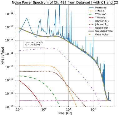
(a) Channel 487, data-set I.

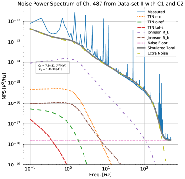
(b) Channel 487, data-set II.

Figure 12: Left: Simulated NPS with estimated $C_{1}$ and $C_{2}$ coefficients for the sample channel 487, compared to measured NPS from data-set I. Right: Simulated NPS with the same estimated $C_{1}$ and $C_{2}$ coefficients, compared to measured NPS from data-set II. We note that the same set of coefficients both produce good agreement with the measurement.

Others [43] have shown similar additional $1/f$ and $f$ noise components that have to be considered in the input spectrum in large resistors:

$$e^{2}_{J-L}=4kTR_{\rm{bias}}+\underbrace{K_{f}}_{R_{\rm{bias}}^{2}C_{1}}f+\underbrace{\beta V^{2}_{\rm{bias}}R_{\rm{bias}}}_{R_{\rm{bias}}^{2}C_{2}}\frac{1}{f}.$$ (5.13)

Specifically, the $R_{\rm{bias}}^{2}C_{2}$ term is voltage and resistance dependent. The bias resistors of CUORE are custom designed to minimize noise and for them, $K_{f}$ and $\beta$ parameters are [43]: $K_{f}=$5\text{\times}{10}^{-13}\text{\,}\mathrm{V}^{2}\mathrm{/}\mathrm{Hz}^{2}$$ and $\beta=$1.96\text{\times}{10}^{-11}\text{\,}\mathrm{\SIUnitSymbolOhm}^{-1}$$. We have found little change in the noise power spectrum with these values. Moreover, we changed the bias resistors to higher values (from $60\text{\,}\mathrm{G\SIUnitSymbolOhm}$ to $240\text{\,}\mathrm{G\SIUnitSymbolOhm}$) in a few channels and saw no appreciable change in the NPS. We have also measured the noise on channel 487’s dummy resistor at room temperature substituting the NTD-Ge. The dummy resistor is $4\text{\,}\mathrm{M\SIUnitSymbolOhm}$ and is under similar bias conditions of the NTD-Ges. The result showed only white noise behavior for the dummy resistor, as shown in Figure 13. These tests suggest that the frequency-dependent noise sources mentioned in eq. (5.9) do not have resistance dependence.

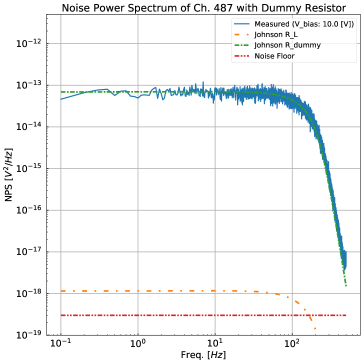
Figure 13: The simulated and measured NPS for channel 487’s $$4\text{\,}\mathrm{[}$]{\mega}$ dummy resistor, along with $R_{\rm{bias}}=$240\text{\,}\mathrm{G\SIUnitSymbolOhm}$$ (labelled $R_{\rm{L}}$) and a total biasing voltage of $$10\text{\,}\mathrm{[}$]{}$. The white noise behavior with the Bessel filter roll-off agrees well with the data.

We should mention that a hypothetical source of excess noise could be vibration heating, as studied in another manuscript [44]. Although the cryogenic set-up of CUORE is very different from the above work, vibrations are known sources of excess noise for low temperature detectors [45]. We integrated the residual noise power in the following frequency bands: 0 to 1 Hz, 1 to 20 Hz, 20 to 250 Hz (excluding 50 Hz and corresponding harmonics) and 250 to 500 Hz. The residual power for sample channels of data-set I is plotted against the floor level in Figure 14.

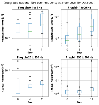
Figure 14: Residual noise power for the sample channels versus detector floor level. Higher floor level corresponds to positions closer to the mixing chamber plate. We note the trend that the closer the channels are to the mixing chamber plate, the more noisy they tend to become. The dots represent outlier channels with excessive integrated noise power.

As the plot shows, the residual power increases with floor level in the detector, which increases when the crystal is closer to cryostat thermal stages. Similar trend is also observed for data-set II. The residual noise in the 20 to 250 Hz band have almost no floor level dependence, suggesting that other noise sources besides the vibrations may have contributed in the band.

It is difficult to ascertain $1/f$ component of the vibration noise from flicker noise ($1/f^{-\gamma}$) because they are both non-stationary and extremely correlated in nature. A detailed analysis of $1/f^{-\gamma}$ noise in our experiment is out of scope for this paper and will be covered in future studies.

6 Conclusion

We have studied both the equilibrium and dynamic states of a macroscopic calorimeter, and have analyzed our model’s consistency from both perspectives. We have confirmed that our three-node thermal model is able to describe the equilibrium state of the detector, and that for the NTD-Ge thermistors used by the CUORE experiment the thermistor resistivity is a function of both the electron temperature and applied bias voltage. We have found that the thermal coupling between the electron gas and the Ge lattice is weaker than expected and dominates the electro-thermal response of the calorimeter.

The dynamic model is able to predict the energy dependent pulse shape up to at least $5407\text{\,}\mathrm{keV}$ with an additional second-order temperature dependence correction term denoted as the $q$ factor. This correction is approximately a few percent when compared to the first order terms. We have made several trials with different models, including ones with more nodes and thermal couplings, and come to the conclusion that the correction term is most likely the effect of a slight change in the NTD-Ge resistivity law, for example an increase of the $\gamma$ factor in eq. (2.13) from the standard value of 0.5. The fit parameters for each channel are close even at two different heat-sink temperatures, indicating that the dynamic model is consistent with the equilibrium model.

As an application of the physical parameters obtained by the model, we have also studied the noise power spectrum for the macro-calorimeters. In the noise analysis, we find excess noise power present in the measurements than expected, and modelled it. Further study is necessary to determine the origin. We, now, have verified that the residual noise power increases with proximity to the mixing chamber and the pulse tubes. Further usage of this model could include the generation of simulated pulses for CUORE to implement a machine-learning pulse energy identifier, and the potential to optimize the detector response in the CUORE Upgrade with Particle ID (CUPID) experiment.

Data Availability

Raw data were generated at the National Energy Research Scientific Computing Center (NERSC) large scale facility. Derived data supporting the findings of this study are available from the corresponding author upon reasonable request.

References

- [1] J. Schechter and J.W.F. Valle, Neutrinoless double- decay in SU(2)×U(1) theories, Physical Review D 25 (1982) 2951.
- [2] M.J. Dolinski, A.W. Poon and W. Rodejohann, Neutrinoless double-beta decay: Status and prospects, Annual Review of Nuclear and Particle Science 69 (2019) 219.
- [3] M. Moe and P. Vogel, Double beta decay, Annual Review of Nuclear and Particle Science 44 (1994) 247.
- [4] J.D. Vergados, H. Ejiri and F. Šimkovic, Neutrinoless double beta decay and neutrino mass, International Journal of Modern Physics E 25 (2016) 1630007 [1612.02924].
- [5] M. Fukugita and T. Yanagida, Barygenesis without grand unification, Physics Letters B 174 (1986) 45.
- [6] M. Martinez, Status of CUORE: An observatory for neutrinoless double beta decay and other rare events, in Proceedings, 12th Patras Workshop on Axions, WIMPs and WISPs (PATRAS 2016): Jeju Island, South Korea, June 20-24, 2016, pp. 112–115, 2017, DOI.
- [7] K. Alfonso, D.R. Artusa, F.T. Avignone, O. Azzolini, M. Balata, T.I. Banks et al., Search for Neutrinoless Double-Beta Decay of 130Te with CUORE-0, Physical Review Letters 115 (2015) .
- [8] The CUORE Collaboration, D.Q. Adams, C. Alduino, K. Alfonso, F.T. Avignone, O. Azzolini et al., Search for Majorana neutrinos exploiting millikelvin cryogenics with CUORE, Nature 604 (2022) 53.
- [9] E. Haller, N. Palaio, M. Rodder, W. Hansen and E. Kreysa, NTD germanium: A novel material for low temperature bolometers, in Neutron Transmutation Doping of Semiconductor Materials, pp. 21–36, Springer (1984).
- [10] N. Wang, F.C. Wellstood, B. Sadoulet, E.E. Haller and J. Beeman, Electrical and thermal properties of neutron-transmutation-doped Ge at 20 mK, Physical Review B 41 (1990) 3761.
- [11] M. Carrettoni and M. Vignati, Signal and noise simulation of CUORE bolometric detectors, Journal of Instrumentation 6 (2011) P08007.
- [12] L. Gironi, Pulse Shape Analysis with Scintillating Bolometers, Journal of Low Temperature Physics 167 (2012) 504.
- [13] D. McCammon, Semiconductor Thermistors, in Cryogenic Particle Detection, C. Enss, ed., (Berlin, Heidelberg), pp. 35–62, Springer Berlin Heidelberg (2005).
- [14] J. Soudée, D. Broszkiewicz, Y. Giraud-Héraud, P. Pari and M. Chapellier, Hot Electrons Effect in a #23 NTD Ge Sample, Journal of Low Temperature Physics 110 (1998) 1013.
- [15] J. Zhang, W. Cui, M. Juda, D. McCammon, R.L. Kelley, S.H. Moseley et al., Non-Ohmic effects in hopping conduction in doped silicon and germanium between 0.05 and 1 K, Physical Review B 57 (1998) 4472.
- [16] M. Piat, J.P. Torre, J.W. Beeman, J.M. Lamarre and R.S. Bhatia, Modelling and Optimizing of High Sensitivity Semiconducting Thermistors at Low Temperature, Journal of Low Temperature Physics 125 (2001) 189.
- [17] M. Galeazzi and D. McCammon, Microcalorimeter and bolometer model, Journal of Applied Physics 93 (2003) 4856.
- [18] E. Figueroa-Feliciano, Complex microcalorimeter models and their application to position-sensitive detectors, Journal of Applied Physics 99 (2006) 114513.
- [19] J.C. Mather, Electrical self-calibration of nonideal bolometers, Applied Optics 23 (1984) 3181.
- [20] J.C. Mather, Bolometer noise: Nonequilibrium theory, Applied Optics 21 (1982) 1125.
- [21] J.C. Mather, Bolometers: Ultimate sensitivity, optimization, and amplifier coupling, Applied Optics 23 (1984) 584.
- [22] R.C. Jones, The general theory of bolometer performance, Journal of The Optical Society of America 43 (1953) 1.
- [23] A. Alessandrello, C. Brofferio, D. Camin, O. Cremonesi, A. Giuliani, M. Pavan et al., An electrothermal model for large mass bolometric detectors, IEEE Transactions on Nuclear Science 40 (1993) 649.
- [24] C. Alduino, K. Alfonso, D. Artusa, F.A. III, O. Azzolini, M. Balata et al., CUORE-0 detector: Design, construction and operation, Journal of Instrumentation 11 (2016) P07009.
- [25] E. Andreotti, C. Arnaboldi, M. Barucci, C. Brofferio, C. Cosmelli, L. Calligaris et al., The low radioactivity link of the CUORE experiment, Journal of Instrumentation 4 (2009) P09003.
- [26] C. Arnaboldi, P. Carniti, L. Cassina, C. Gotti, X. Liu, M. Maino et al., A front-end electronic system for large arrays of bolometers, Journal of Instrumentation 13 (2018) P02026.
- [27] M. Vignati, Model of the Response Function of CUORE Bolometers, Ph.D. thesis, Sapienza Università di Roma, Dec., 2009.
- [28] M. Pedretti, The Single Module for CUORICINO and CUORE Detectors: Tests, Construction, and Modelling, Ph.D. thesis, Università degli Studi dell’Insubria, Mar., 2004.
- [29] E. Olivieri, M. Barucci, J. Beeman, L. Risegari and G. Ventura, Excess Heat Capacity in NTD Ge Thermistors, Journal of Low Temperature Physics 143 (2006) 153.
- [30] É. Aubourg, A. Cummings, T. Shutt, W. Stockwell, P.D. Barnes, A. Da Silva et al., Measurement of Electron-Phonon Decoupling Time in Neutron-Transmutation Doped Germanium at 20 mK, Journal of Low Temperature Physics 93 (1993) 289.
- [31] P.H. Keesom and G. Seidel, Specific Heat of Germanium and Silicon at Low Temperatures, Physical Review 113 (1959) 33.
- [32] G. Ventura and L. Risegari, The Art of Cryogenics: Low-Temperature Experimental Techniques, Elsevier, Amsterdam ; Boston, 1st ed ed. (2008).
- [33] M. Barucci, C. Brofferio, A. Giuliani, E. Gottardi, I. Peroni and G. Ventura, Measurement of Low Temperature Specific Heat of Crystalline TeO2 for the Optimization of Bolometric Detectors, Journal of Low Temperature Physics 123 (2001) 303.
- [34] V. Singh, A. Garai, S. Mathimalar, N. Dokania, V. Nanal, R. Pillay et al., Specific heat of Teflon, Torlon 4203 and Torlon 4301 in the range of 30–400mK, Cryogenics 67 (2015) 15.
- [35] I. Nutini, The CUORE Experiment: Detector Optimization and Modelling and CPT Conservation Limit, Ph.D. thesis, Gran Sasso Science Institute, Oct., 2018.
- [36] K. Alfonso, C. Bucci, L. Canonica, P. Carniti, S. Di Domizio, A. Giachero et al., A highly automated system to define the best operating settings of cryogenic calorimeters, July, 2020.
- [37] A.L. Efros and B.I. Shklovskii, Coulomb gap and low temperature conductivity of disordered systems, Journal of Physics C: Solid State Physics 8 (1975) L49.
- [38] D. McCammon, Thermal Equilibrium Calorimeters – An Introduction, in Cryogenic Particle Detection, C. Enss, ed., (Berlin, Heidelberg), pp. 1–34, Springer Berlin Heidelberg (2005), DOI.
- [39] R.M. Hill, Hopping conduction in amorphous solids, Philosophical Magazine 24 (1971) 1307.
- [40] T.W. Kenny, P.L. Richards, I.S. Park, E.E. Haller and J.W. Beeman, Bias-induced nonlinearities in the dc I-V characteristics of neutron-transmutation-doped germanium at liquid 4He temperatures, Physical Review B 39 (1989) 8476.
- [41] P. Virtanen, R. Gommers, T.E. Oliphant, M. Haberland, T. Reddy, D. Cournapeau et al., SciPy 1.0: Fundamental algorithms for scientific computing in python, Nature Methods 17 (2020) 261.
- [42] C. Rusconi, Optimization of the bolometric performances of the CUORE-0/CUORE and LUCIFER detectors for the neutrinoless double beta decay search, Ph.D. thesis, Insubria U., Varese, July, 2011.
- [43] C. Amaboldi, C. Bucci, O. Cremonesi, A. Fascilla, A. Nucciotti, M. Pavan et al., Low-Frequency Noise Characterization of Very Large Value Resistors, IEEE Transactions on Nuclear Science 49 (2002) 1808.
- [44] S. Pirro, A. Alessandrello, C. Brofferio, C. Bucci, O. Cremonesi, E. Coccia et al., Vibrational and thermal noise reduction for cryogenic detectors, Nuclear Instruments and Methods in Physics Research Section A: Accelerators, Spectrometers, Detectors and Associated Equipment 444 (2000) 331.
- [45] A. D’Addabbo, C. Bucci, L. Canonica, S. Di Domizio, P. Gorla, L. Marini et al., An active noise cancellation technique for the CUORE Pulse Tube Cryocoolers, Cryogenics 93 (2018) 56.