A hybridizable discontinuous Galerkin method for the fully coupled time-dependent Stokes/Darcy–transport problem

Abstract.

We present a high-order hybridized discontinuous Galerkin (HDG) method for the fully coupled time-dependent Stokes–Darcy-transport problem where the fluid viscosity and source/sink terms depend on the concentration and the dispersion/diffusion tensor depends on the fluid velocity. This HDG method is such that the discrete flow equations are compatible with the discrete transport equation. Furthermore, the HDG method guarantees strong mass conservation in the $H^{\rm div}$ sense and naturally treats the interface conditions between the Stokes and Darcy regions via facet variables. We employ a linearizing decoupling strategy where the Stokes/Darcy and the transport equations are solved sequentially by time-lagging the concentration. We prove well-posedness and optimal a priori error estimates for the velocity and the concentration in the energy norm. We present numerical examples that respect compatibility of the flow and transport discretizations and demonstrate that the discrete solution is robust with respect to the problem parameters.

1. Introduction

Coupled free fluid and porous media flow is encountered in many engineering applications [24, 34] and can be modeled by the Stokes/Darcy equations. Adding a transport equation to this coupled system brings forth a model that can be used to simulate the spread of contaminants towards groundwater resources [4] or biochemical transport in hemodynamics [21].

The accuracy and stability of numerical discretizations of the stationary Stokes/Darcy equations [25, 37, 11, 13, 12, 3, 29, 39, 41] and advection-diffusion type transport equations [40, 10, 20, 52] are well studied. However, accuracy and stability are not automatically guaranteed when these discretizations are coupled. In particular, compatible discretizations, as defined by [22], are desired to avoid loss of accuracy and loss of conservation properties of the numerical methods used for the transport equation.

The first numerical study on the coupling of the stationary Stokes/Darcy equations with a transport equation was given in [51] where a mixed finite element method (MFEM) is used for the flow problem and the local discontinuous Galerkin method is used for the transport problem. They considered one-way coupling; the concentration is affected by the flow velocity, but the velocity is not affected by a change in concentration. The same problem was studied in [43] by using discontinuous Galerkin (DG) methods for both flow and transport equations. In [28], Ervin et. al considered a fully time-dependent version of the one-way coupled problem where they developed partitioned time-stepping methods by imposing the interface conditions weakly using penalties. One-way coupling was considered also in [16] in which the flow problem was discretized by a strongly mass conservative Embedded-Hybridized DG (EDG-HDG) method while the transport equation was discretized by an EDG method.

Less studied is the fully-coupled problem in which, apart from the transport equation depending on the flow velocity, the flow solution is time-dependent and the fluid viscosity and source/sink terms depend on the concentration. To the best of our knowledge, there are only two papers that focus on this fully coupled problem. First, [14] presented an analysis of a weak solution for the case where free flow is governed by the Navier–Stokes equations. The analysis in [14], however, also holds when free flow is governed by the Stokes equations. The only numerical paper on this topic, [45], introduced a stabilized mixed finite element method using nonconforming piece-wise linear Crouzeix–Raviart finite elements for the velocity, a piece-wise constant approximation for the pressure, and a conforming, piece-wise linear, finite element method for the transport equation based on a skew-symmetric formulation.

In this paper, we extend the work in [16] to the fully coupled case. To deal with the non-linearity, we consider a linearizing decoupling strategy, where the Stokes/Darcy and the transport equations are solved sequentially by time-lagging the concentration. We use HDG methods [19] for both the Stokes/Darcy and transport sub-problems at each time step and prove well-posedness and a priori error estimates. These results can easily be extended to the EDG-HDG discretization used for the Stokes/Darcy problem in [16]. Our HDG method for the flow problem provides the transport sub-problem at each time step with an exactly mass conserving and $H({\rm div})$-conforming velocity field. This renders our scheme robust with respect to the problem parameters. By choosing the polynomial degree in a specific way our flow/transport scheme is also compatible.

Here is an outline for the remainder of this article. In Section 2, we present the fully coupled Stokes/Darcy-transport model and specify the assumptions on the problem parameters. Section 3 sets notation, describes in detail the semi-discrete HDG scheme, and lists the attractive properties of the numerical discretization. Next, Section 4 summarizes standard inequalities and shows continuity, coercivity, and the inf-sup condition for the discretization of the Stokes/Darcy sub-problem. A full discretization of the problem based on a sequential decoupling strategy is introduced in Section 5 while the main results, i.e., a priori error estimates for the velocity, pressure, and concentration, are presented in Section 6. Finally, we present some numerical experiments in Section 7 followed by conclusions in Section 8.

2. The Stokes/Darcy–transport system

Let $\Omega\subset\mathbb{R}^{\dim}$, ${\dim}=2,3$, be a bounded polygonal domain.

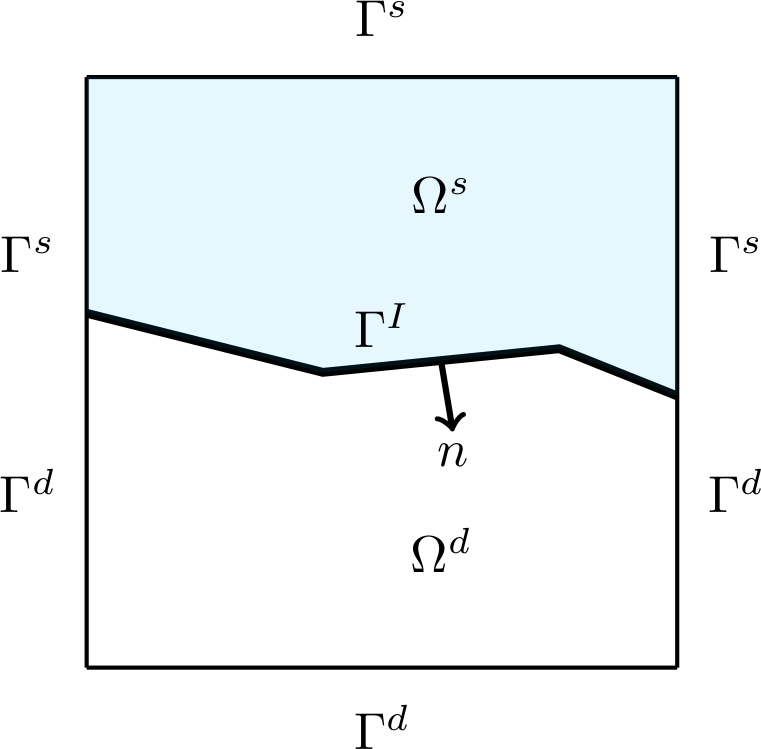
Figure 1. A depiction of a domain $\Omega\subset\mathbb{R}^{2}$ with its two sub-domains $\Omega^{s}$ and $\Omega^{d}$.

We denote its boundary by $\partial\Omega$ and the outward unit normal to $\partial\Omega$ by $n$. Domain $\Omega$ consists of two non-overlapping polygonal regions, a free flow region $\Omega^{s}$ and a Darcy flow region $\Omega^{d}$, such that $\Omega=\Omega^{s}\cup\Omega^{d}$. The polygonal interface between $\Omega^{s}$ and $\Omega^{d}$ is denoted by $\Gamma^{I}$ and the external boundary of $\Omega^{j}$ is denoted by $\Gamma^{j}\mathrel{\mathop{\mathchar 58\relax}}=\partial\Omega\cap\partial\Omega^{j}$, $j=s,d$. See Figure 1 for a depiction of a domain when ${\dim}=2$.

We denote the time interval of interest by $J=[0,T]$. The fully coupled Stokes/Darcy–transport system for the velocity field $u\mathrel{\mathop{\mathchar 58\relax}}\Omega\times J\to\mathbb{R}^{\dim}$, fluid pressure $p\mathrel{\mathop{\mathchar 58\relax}}\Omega\times J\to\mathbb{R}$ and concentration $c\mathrel{\mathop{\mathchar 58\relax}}\Omega\times J\rightarrow\mathbb{R}$ is given by

$$\partial_{t}u-\nabla\cdot(2\mu(c)\varepsilon(u))+\nabla p =f^{s}(c) \text{in}\ \Omega^{s}\times J,$$ (1a)

$$\mathbb{K}^{-1}(c)u+\nabla p =\mathbb{K}^{-1}(c)f^{d}(c) \text{in}\ \Omega^{d}\times J,$$ (1b)

$$-\nabla\cdot u =\raisebox{2.0pt}{$\chi$}_{d}(g_{p}-g_{i}) \text{in}\ \Omega\times J,$$ (1c)

$$\phi\partial_{t}c+\nabla\cdot(cu-\widetilde{D}(u)\nabla c) =\raisebox{2.0pt}{$\chi$}_{d}(c_{I}g_{i}-cg_{p}) \text{in}\ \Omega\times J,$$ (1d)

$$u =0 \text{on}\ \Gamma^{s}\times J,$$ (1e)

$$u\cdot n =0 \text{on}\ \Gamma^{d}\times J,$$ (1f)

$$\widetilde{D}(u)\nabla c\cdot n =0 \text{on}\ \partial\Omega\times J,$$ (1g)

where $\varepsilon(u)\mathrel{\mathop{\mathchar 58\relax}}=\mathinner{\left(\nabla u+(\nabla u)^{T}\right)}/2$ is the strain rate tensor and $\raisebox{2.0pt}{$\chi$}_{d}$ is the characteristic function that takes the value 1 in $\Omega^{d}$ and 0 in $\Omega^{s}$. Here the fluid viscosity $\mu$, the matrix $\mathbb{K}=\frac{\kappa}{\mu}$, where $\kappa$ is the permeability matrix of the porous medium, and the body force terms $f^{s}$ and $f^{d}$ are concentration dependent functions. The porosity $\phi$ of the medium in $\Omega^{d}$ is a spatially varying function. In $\Omega^{s}$ we set $\phi=1$. The functions $g_{i}$ and $g_{p}$ denote the source and sink terms related to injection and production wells and $c_{I}$ is the injected concentration. Furthermore, in the Stokes region $\widetilde{D}(u)=d\mathbb{I}$, where $\mathbb{I}$ is the $\dim\times\dim$ identity matrix and $d$ is the diffusion coefficient. In the Darcy region $\widetilde{D}(u)=D(u)$, where $D(u)$ denotes the diffusion dispersion tensor in $\Omega^{d}$.

We will denote the restriction of the velocity $u$, pressure $p$, and concentration $c$ to sub-domain $\Omega^{j}$, $j=s,d$ by, respectively, $u^{j}$, $p^{j}$, and $c^{j}$. Then, on the interface $\Gamma^{I}$, choosing the unit normal vector $n$ to be pointing from $\Omega^{s}$ to $\Omega^{d}$, we prescribe the following interface conditions that hold for $t\in J$:

$$u^{s}\cdot n =u^{d}\cdot n,$$ (2a)

$$p^{s}-(2\mu(c^{s})\varepsilon(u^{s})n)\cdot n =p^{d},$$ (2b)

$$-2(\varepsilon(u^{s})n)\cdot\tau^{\ell} =\gamma^{\ell}u^{s}\cdot\tau^{\ell},\quad\ell=1,\ldots,{\dim}-1,$$ (2c)

$$c^{s} =c^{d},$$ (2d)

$$d\nabla c^{s}\cdot n =D(u^{d})\nabla c^{d}\cdot n,$$ (2e)

where $\tau^{\ell}$, $\ell=1,\ldots,{\dim}-1$ denote the unit tangent vectors on $\Gamma^{I}$. These conditions enforce the normal continuity of the velocity (2a), the normal continuity of the normal component of the stress (2b), continuity of the concentration (2d), and normal continuity of the concentration flux (2e). Equation 2c, where $\gamma^{\ell}=\alpha/\sqrt{\tau^{\ell}\cdot\kappa\tau^{\ell}}$ with $\alpha>0$ a constant, is the Beavers–Joseph–Saffman law which enforces a condition on the tangential component of the normal stress [5, 46].

To close the model, we assume the following initial conditions:

$$u^{s}(x,0) =u^{s}_{0}(x) \text{in}\ \Omega^{s},$$ (3a)

$$c(x,0) =c_{0}(x) \text{in}\ \Omega.$$ (3b)

We end this section by discussing some assumptions we make on the various functions used in the Stokes/Darcy–transport model. The dispersion-diffusion tensor $D(u)$ in $\Omega^{d}$ satisfies for $u,v\in\mathbb{R}^{\dim}$:

$$D_{\min}|\xi|^{2} \leq\xi^{T}D(u)\xi\quad\forall\xi\in\mathbb{R}^{\dim},$$ (4a)

$$|D(u)| \leq C(1+\mathinner{\!\left\lvert u\right\rvert}),$$ (4b)

$$\mathinner{\!\left\lvert D(u)-D(v)\right\rvert} \leq C\mathinner{\!\left\lvert u-v\right\rvert},$$ (4c)

where $D_{\min}$ and $C$ are positive constants and $|\cdot|$ denotes the Euclidean norm. We assume that $\mu$ is Lipschitz continuous in $c$ with Lipschitz constant $\mu_{L}$ and that there exist constants $\phi_{*},\phi^{*},\mu_{*},\mu^{*}>0$ such that

$$\phi_{*}\leq\phi(x) \leq\phi^{*} \forall x\in\Omega^{d},$$ (5a)

$$\mu_{*}\leq\mu(c) \leq\mu^{*} \forall c\in\mathbb{R}.$$ (5b)

The permeability matrix $\kappa$ is symmetric, uniformly bounded, and elliptic, that is, there exist positive constants $\kappa_{*}<\kappa^{*}$ such that

$$\kappa_{*}|\xi|^{2}\leq\xi^{T}\kappa(x)\xi\leq\kappa^{*}|\xi|^{2}\quad\forall\xi\in\mathbb{R}^{\dim},\quad\forall x\in\bar{\Omega}^{d}.$$ (6)

From (6) and (5b), we deduce that

$$K_{*}|\xi|^{2}\leq\xi^{T}\mathbb{K}(c,x)\xi\leq K^{*}|\xi|^{2}\quad\forall\xi\in\mathbb{R}^{\dim},\quad\forall(c,x)\in\mathbb{R}\times\bar{\Omega}^{d},$$ (7)

where $K_{*}=\kappa_{*}/\mu^{*}$ and $K^{*}=\kappa^{*}/\mu_{*}$.

The body force functions $f^{s}$ and $f^{d}$ are assumed to be Lipschitz continuous in $c$ with Lipschitz constants $L_{f}^{s}$ and $L_{f}^{d}$. Note that $f^{s}$ and $f^{d}$ depend on $x$ and $c$, but they do not depend explicitly on $t$. We will further assume that $0\leq c_{I}\leq 1$ a.e. in $\Omega^{d}$ and that $g_{i},g_{p}\geq 0$, $g_{i},g_{p}\in L^{\infty}(J;L^{2}(\Omega^{d}))$ are such that

$$\int_{\Omega^{d}}(g_{i}(x,t)-g_{p}(x,t))\operatorname{d\!}x=0\quad\forall t\in J.$$

A weak formulation of the problem defined by eqs. 1, 2 and 3 was presented in [45]. The analysis for a weak solution of a more general version of this problem, in which the free fluid flow is governed by the Navier–Stokes equations, can be found in [14].

3. The hybridized discontinuous Galerkin method

3.1. Preliminaries

We use the same notation that we used previously in [17, 16]. Let $\mathcal{T}^{j}\mathrel{\mathop{\mathchar 58\relax}}=\mathinner{\left\{K\right\}}$ be a shape-regular triangulation of $\Omega^{j}$, $j=s,d$, into non-overlapping elements (we only consider simplices) such that $\mathcal{T}^{s}$ and $\mathcal{T}^{d}$ match at the interface $\Gamma^{I}$. We define the triangulation of the entire domain $\Omega$ as $\mathcal{T}\mathrel{\mathop{\mathchar 58\relax}}=\mathcal{T}^{s}\cup\mathcal{T}^{d}$. The maximum diameter over all elements is $h=\max_{K\in\mathcal{T}}h_{K}$, where $h_{K}$ stands for the diameter of an element $K$. The boundary of an element $K$ and its outward unit normal are denoted by $\partial K$ and $n$, respectively. A facet of an element boundary is an interior facet if it is shared by two neighboring elements and it is a boundary facet if it is a part of $\partial\Omega$. The set of all interior facets and all boundary facets in $\bar{\Omega}^{j}$ are denoted by $\mathcal{F}_{i}^{j}$ and $\mathcal{F}_{b}^{j}$, $j=s,d$, respectively. We also collect the facets that lie on the interface $\Gamma^{I}$ in the set $\mathcal{F}^{I}$. The set of all facets that lie in $\bar{\Omega}$ and in $\bar{\Omega}^{j}$ are denoted by $\mathcal{F}$ and $\mathcal{F}^{j}$, respectively. We point out that $\mathcal{F}^{j}=\mathcal{F}_{i}^{j}\cup\mathcal{F}_{b}^{j}\cup\mathcal{F}^{I}$, $j=s,d$. Furthermore, we define $\Gamma_{0}\mathrel{\mathop{\mathchar 58\relax}}=\cup_{F\in\mathcal{F}}F$ and $\Gamma_{0}^{j}\mathrel{\mathop{\mathchar 58\relax}}=\cup_{F\in\mathcal{F}^{j}}F$, $j=s,d$.

The finite element function spaces on $\Omega$ for the velocity and pressure are given by

$$\begin{split}V_{h}&\mathrel{\mathop{\mathchar 58\relax}}=\mathinner{\bigl{\{}v_{h}\in\mathinner{[L^{2}(\Omega)]}^{\dim}\mathrel{\mathop{\mathchar 58\relax}}\ v_{h}\in\mathinner{[P_{k_{f}}(K)]}^{\dim},\ \forall\ K\in\mathcal{T}\bigr{\}}},\\ Q_{h}&\mathrel{\mathop{\mathchar 58\relax}}=\mathinner{\bigl{\{}q_{h}\in L^{2}(\Omega)\mathrel{\mathop{\mathchar 58\relax}}\ q_{h}\in P_{k_{f}-1}(K),\ \forall\ K\in\mathcal{T}\bigr{\}}}\cap L^{2}_{0}(\Omega),\end{split}$$ (8)

where $P_{k}(K)$ denotes the space of polynomials of degree at most $k$ defined on the element $K$. The finite element spaces for the velocity and pressure traces are given by

$$\begin{split}\bar{V}_{h}&\mathrel{\mathop{\mathchar 58\relax}}=\mathinner{\bigl{\{}\bar{v}_{h}\in\mathinner{[L^{2}(\Gamma_{0}^{s})]}^{\dim}\mathrel{\mathop{\mathchar 58\relax}}\ \bar{v}_{h}\in\mathinner{[P_{k_{f}}(F)]}^{\dim}\ \forall\ F\in\mathcal{F}^{s},\ \bar{v}_{h}=0\ \mbox{on}\ \Gamma^{s}\bigr{\}}},\\ \bar{Q}_{h}^{j}&\mathrel{\mathop{\mathchar 58\relax}}=\mathinner{\bigl{\{}\bar{q}_{h}^{j}\in L^{2}(\Gamma_{0}^{j})\mathrel{\mathop{\mathchar 58\relax}}\ \bar{q}_{h}^{j}\in P_{k_{f}}(F)\ \forall\ F\in\mathcal{F}^{j}\bigr{\}}},\quad j=s,d.\end{split}$$ (9)

Here $P_{k}(F)$ denotes the space of polynomials of degree at most $k$ defined on the facet $F$. Note that functions in $\bar{V}_{h}$ are not defined on $\Gamma_{0}^{d}\backslash\Gamma_{I}$. The finite element function spaces for the concentration and its trace are defined as

$$\begin{split}C_{h}=\mathinner{\{c_{h}\in L^{2}(\Omega)\mathrel{\mathop{\mathchar 58\relax}}\ c_{h}\in P_{k_{c}}(K),\ \forall\ K\in\mathcal{T}\}},\quad\bar{C}_{h}=\mathinner{\{\bar{c}_{h}\in L^{2}(\Gamma_{0})\mathrel{\mathop{\mathchar 58\relax}}\ \bar{c}_{h}\in P_{k_{c}}(F)\ \forall\ F\in\mathcal{F}\}}.\end{split}$$ (10)

The semi-discrete and fully-discrete HDG methods for the flow and transport equations considered in this article are compatible when $k_{c}=k_{f}-1$ [16]. For this reason we set $k_{c}=k_{f}-1$.

To reduce the notational burden, we define $\boldsymbol{V}_{h}\mathrel{\mathop{\mathchar 58\relax}}=V_{h}\times\bar{V}_{h}$, $\boldsymbol{Q}_{h}\mathrel{\mathop{\mathchar 58\relax}}=Q_{h}\times\bar{Q}_{h}^{s}\times\bar{Q}_{h}^{d}$, and $\boldsymbol{Q}_{h}^{j}\mathrel{\mathop{\mathchar 58\relax}}=Q_{h}^{j}\times\bar{Q}_{h}^{j}$, $j=s,d$. We denote elements in these product spaces by $\boldsymbol{v}_{h}\mathrel{\mathop{\mathchar 58\relax}}=(v_{h},\bar{v}_{h})\in\boldsymbol{V}_{h}$, $\boldsymbol{q}_{h}\mathrel{\mathop{\mathchar 58\relax}}=(q_{h},\bar{q}_{h}^{s},\bar{q}_{h}^{d})\in\boldsymbol{Q}_{h}$, and $\boldsymbol{q}_{h}^{j}\mathrel{\mathop{\mathchar 58\relax}}=(q_{h}^{j},\bar{q}_{h}^{j})\in\boldsymbol{Q}_{h}^{j}$, $j=s,d$. In addition, we set $\boldsymbol{X}_{h}\mathrel{\mathop{\mathchar 58\relax}}=\boldsymbol{V}_{h}\times\boldsymbol{Q}_{h}$. Similarly, we introduce $\boldsymbol{C}_{h}=C_{h}\times\bar{C}_{h}$ and denote the corresponding elements by $\boldsymbol{c}_{h}\mathrel{\mathop{\mathchar 58\relax}}=(c_{h},\bar{c}_{h})\in\boldsymbol{C}_{h}$.

Next, let us define the function spaces

$$V \mathrel{\mathop{\mathchar 58\relax}}=\big{\{}v\in[L^{2}(\Omega)]^{\dim}\ \mathrel{\mathop{\mathchar 58\relax}}\ v^{s}\in\mathinner{[H^{2}(\Omega^{s})]}^{\dim},\ v^{d}\in\mathinner{[H^{1}(\Omega^{d})]}^{\dim},$$

$$\hskip 99.58464ptv=0\ \text{on}\ \Gamma^{s},\ v\cdot n=0\ \text{on}\ \Gamma^{d},\ v^{s}\cdot n=v^{d}\cdot n\ \text{on}\ \Gamma^{I}\big{\}},$$

$$Q \mathrel{\mathop{\mathchar 58\relax}}=\big{\{}q\in L_{0}^{2}(\Omega)\ \mathrel{\mathop{\mathchar 58\relax}}\ q^{s}\in H^{1}(\Omega^{s}),\ q^{d}\in H^{2}(\Omega^{d})\big{\}},$$

$$C \mathrel{\mathop{\mathchar 58\relax}}=H^{2}(\Omega),$$

and set $X\mathrel{\mathop{\mathchar 58\relax}}=V\times Q$. As before, we use a superscript ^j to specify the restriction of these spaces to $\Omega^{j}$, $j=s,d$. The trace spaces of $V$ restricted to $\Gamma_{0}^{s}$, $Q^{j}$ restricted to $\Gamma_{0}^{j}$, and $C$ restricted to $\Gamma_{0}$ are denoted by, respectively, $\bar{V}$, $\bar{Q}^{j}$, and $\bar{C}$. The trace operator $\gamma_{V}\mathrel{\mathop{\mathchar 58\relax}}V^{s}\to\bar{V}$ restricts functions in $V^{s}$ to $\Gamma_{0}^{s}$, and similarly the trace operators $\gamma_{Q^{j}}\mathrel{\mathop{\mathchar 58\relax}}Q^{j}\to\bar{Q}^{j}$ restrict functions in $Q^{j}$ to $\Gamma_{0}^{j}$, $j=s,d$. However, when it is clear from the context, we omit the subscript in the trace operator. Analogous to the discrete case, we introduce $\boldsymbol{V}\mathrel{\mathop{\mathchar 58\relax}}=V\times\bar{V}$, $\boldsymbol{Q}\mathrel{\mathop{\mathchar 58\relax}}=Q\times\bar{Q}^{s}\times\bar{Q}^{d}$, and $\boldsymbol{C}\mathrel{\mathop{\mathchar 58\relax}}=C\times\bar{C}$. We then define extended function spaces as

$$\boldsymbol{V}(h)\mathrel{\mathop{\mathchar 58\relax}}=\boldsymbol{V}_{h}+\boldsymbol{V},\quad\boldsymbol{Q}(h)\mathrel{\mathop{\mathchar 58\relax}}=\boldsymbol{Q}_{h}+\boldsymbol{Q},\quad\boldsymbol{C}(h)\mathrel{\mathop{\mathchar 58\relax}}=\boldsymbol{C}_{h}+\boldsymbol{C},$$

and set $\boldsymbol{X}(h)\mathrel{\mathop{\mathchar 58\relax}}=\boldsymbol{V}(h)\times\boldsymbol{Q}(h)$.

We close this section by listing various norms on the spaces described above. We refer the reader to [1] for the definitions of the standard Sobolev spaces $W^{m,p}(D)$ and their corresponding norms $\|\cdot\|_{W^{m,p}(D)}$. For ease of notation, we write $\|\cdot\|_{m,p,D}$ instead of $\|\cdot\|_{W^{m,p}(D)}$ with the following simplifications. When $m=0$, $W^{0,p}(D)$ coincides with $L^{p}(D)$ and when $p=2$, $H^{m}(D)=W^{m,p}(D)$. For $p=2$, we write $\|\cdot\|_{m,D}$ to denote $\|\cdot\|_{W^{m,2}(D)}$ and for $m=0$, $p=2$, we write $\|\cdot\|_{D}$ instead of $\|\cdot\|_{0,D}$.

On $\boldsymbol{V}^{s}(h)$ we define the standard HDG-norm and its strengthened version as follows:

$$\mathopen{|\mkern-1.5mu|\mkern-1.5mu|}\boldsymbol{v}\mathclose{|\mkern-1.5mu|\mkern-1.5mu|}_{v,s}^{2}\mathrel{\mathop{\mathchar 58\relax}}=\sum_{K\in\mathcal{T}^{s}}\mathinner{\bigl{(}\mathinner{\lVert\nabla v\rVert}_{K}^{2}+h_{K}^{-1}\mathinner{\!\left\lVert v-\bar{v}\right\rVert}^{2}_{\partial K}\bigr{)}},\quad\mathopen{|\mkern-1.5mu|\mkern-1.5mu|}\boldsymbol{v}\mathclose{|\mkern-1.5mu|\mkern-1.5mu|}_{v^{\prime},s}^{2}\mathrel{\mathop{\mathchar 58\relax}}=\mathopen{|\mkern-1.5mu|\mkern-1.5mu|}\boldsymbol{v}\mathclose{|\mkern-1.5mu|\mkern-1.5mu|}_{v,s}^{2}+\sum_{K\in\mathcal{T}^{s}}h_{K}^{2}\mathinner{\!\left\lvert v\right\rvert}_{H^{2}(K)}^{2}.$$

On $\boldsymbol{V}(h)$ we then introduce the norms

$$\begin{split}\mathopen{|\mkern-1.5mu|\mkern-1.5mu|}\boldsymbol{v}\mathclose{|\mkern-1.5mu|\mkern-1.5mu|}_{v}^{2}&\mathrel{\mathop{\mathchar 58\relax}}=\mathopen{|\mkern-1.5mu|\mkern-1.5mu|}\boldsymbol{v}\mathclose{|\mkern-1.5mu|\mkern-1.5mu|}_{v,s}^{2}+\mathinner{\!\left\lVert v\right\rVert}_{\Omega^{d}}^{2}+\sum_{j=1}^{\dim}\gamma^{j}\|\bar{v}\cdot\tau_{j}\|^{2}_{\Gamma^{I}},\\ \mathopen{|\mkern-1.5mu|\mkern-1.5mu|}\boldsymbol{v}\mathclose{|\mkern-1.5mu|\mkern-1.5mu|}_{v^{\prime}}^{2}&\mathrel{\mathop{\mathchar 58\relax}}=\mathopen{|\mkern-1.5mu|\mkern-1.5mu|}\boldsymbol{v}\mathclose{|\mkern-1.5mu|\mkern-1.5mu|}_{v}^{2}+\sum_{K\in\mathcal{T}^{s}}h_{K}^{2}\mathinner{\!\left\lvert v\right\rvert}_{H^{2}(K)}^{2}=\mathopen{|\mkern-1.5mu|\mkern-1.5mu|}\boldsymbol{v}\mathclose{|\mkern-1.5mu|\mkern-1.5mu|}_{v^{\prime},s}^{2}+\mathinner{\!\left\lVert v\right\rVert}_{\Omega^{d}}^{2}+\sum_{j=1}^{\dim}\gamma^{j}\|\bar{v}\cdot\tau_{j}\|^{2}_{\Gamma^{I}},\end{split}$$

and note that $\mathopen{|\mkern-1.5mu|\mkern-1.5mu|}\boldsymbol{v}\mathclose{|\mkern-1.5mu|\mkern-1.5mu|}_{v}$ and $\mathopen{|\mkern-1.5mu|\mkern-1.5mu|}\boldsymbol{v}\mathclose{|\mkern-1.5mu|\mkern-1.5mu|}_{v^{\prime}}$ are equivalent on $\boldsymbol{V}_{h}$ due to the fact that $\mathopen{|\mkern-1.5mu|\mkern-1.5mu|}\cdot\mathclose{|\mkern-1.5mu|\mkern-1.5mu|}_{v,s}$ and $\mathopen{|\mkern-1.5mu|\mkern-1.5mu|}\cdot\mathclose{|\mkern-1.5mu|\mkern-1.5mu|}_{v^{\prime},s}$ are equivalent on $\boldsymbol{V}_{h}^{s}$ (see, for example, [52, eq. (5.5)]).

On the pressure spaces $\boldsymbol{Q}^{j}(h)$, $j=s,d$ and $\boldsymbol{Q}(h)$, we define, respectively,

$$\mathopen{|\mkern-1.5mu|\mkern-1.5mu|}\boldsymbol{q}^{j}\mathclose{|\mkern-1.5mu|\mkern-1.5mu|}_{p,j}^{2}\mathrel{\mathop{\mathchar 58\relax}}=\mathinner{\!\left\lVert q\right\rVert}_{\Omega^{j}}^{2}+\sum_{K\in\mathcal{T}^{j}}h_{K}\mathinner{\lVert\bar{q}^{j}\rVert}_{\partial K}^{2},\qquad\mathopen{|\mkern-1.5mu|\mkern-1.5mu|}\boldsymbol{q}\mathclose{|\mkern-1.5mu|\mkern-1.5mu|}_{p}^{2}\mathrel{\mathop{\mathchar 58\relax}}=\sum_{j=s,d}\mathopen{|\mkern-1.5mu|\mkern-1.5mu|}\boldsymbol{q}^{j}\mathclose{|\mkern-1.5mu|\mkern-1.5mu|}^{2}_{p,j}.$$

Finally, for $\boldsymbol{w}_{h}\in\boldsymbol{C}(h)$, we define the following semi-norm:

$$\mathopen{|\mkern-1.5mu|\mkern-1.5mu|}\boldsymbol{w}_{h}\mathclose{|\mkern-1.5mu|\mkern-1.5mu|}_{c}^{2}=\sum\limits_{K\in\mathcal{T}}(\|\nabla w_{h}\|_{K}^{2}+h_{K}^{-1}\|w_{h}-\bar{w}_{h}\|_{\partial K}^{2}).$$ (11)

3.2. Semi-discrete HDG scheme

The semi-discrete method we propose for the Stokes/Darcy–transport system in eqs. 1 and 2 is as follows: for $t>0$, find $\big{(}\boldsymbol{u}_{h}(t),\boldsymbol{p}_{h}(t)\big{)}\in\boldsymbol{X}_{h}$ and $\boldsymbol{c}_{h}(t)\in\boldsymbol{C}_{h}$ such that

$$\sum_{K\in\mathcal{T}^{s}}\int_{K}\partial_{t}u_{h}\cdot v_{h}\operatorname{d\!}x+B_{h}^{sd}(\boldsymbol{c}_{h};(\boldsymbol{u}_{h},\boldsymbol{p}_{h}),(\boldsymbol{v}_{h},\boldsymbol{q}_{h}))=\sum_{K\in\mathcal{T}^{s}}\int_{K}f^{s}(c_{h})\cdot v_{h}\operatorname{d\!}x\\ +\sum_{K\in\mathcal{T}^{d}}\int_{K}\mathbb{K}^{-1}(c_{h})f^{d}(c_{h})\cdot v_{h}\operatorname{d\!}x+\sum_{K\in\mathcal{T}^{d}}\int_{K}(g_{p}-g_{i})\,q_{h}\operatorname{d\!}x$$ (12a)

and

$$\sum_{K\in\mathcal{T}}\int_{K}\phi\,\partial_{t}c_{h}w_{h}\operatorname{d\!}x+B_{h}^{tr}(u_{h};\boldsymbol{c}_{h},\boldsymbol{w}_{h})+\sum_{K\in\mathcal{T}^{d}}\int_{K}c_{h}\,g_{p}\,w_{h}\operatorname{d\!}x=\sum_{K\in\mathcal{T}^{d}}\int_{K}c_{I}\,g_{i}\,w_{h}\operatorname{d\!}x,$$ (12b)

for all $\big{(}\boldsymbol{v}_{h},\boldsymbol{q}_{h}\big{)}\in\boldsymbol{X}_{h}$ and $\boldsymbol{w}_{h}\in\boldsymbol{C}_{h}$.

The form $B_{h}^{sd}$ in eq. 12a collects the discretization terms for the Stokes/Darcy momentum and mass conservation equations as follows:

$$B_{h}^{sd}(\boldsymbol{c};(\boldsymbol{u},\boldsymbol{p}),(\boldsymbol{v},\boldsymbol{q}))\mathrel{\mathop{\mathchar 58\relax}}=a_{h}(\boldsymbol{c};\boldsymbol{u},\boldsymbol{v})+\sum_{j=s,d}\mathinner{\left(b_{h}^{j}(\boldsymbol{p}^{j},v)+b_{h}^{I,j}(\bar{p}^{j},\bar{v})\right)}+\sum_{j=s,d}\mathinner{\left(b_{h}^{j}(\boldsymbol{q}^{j},u)+b_{h}^{I,j}(\bar{q}^{j},\bar{u})\right)}.$$ (13)

Here $a_{h}(\cdot,\cdot)$ is defined as

$$a_{h}(\boldsymbol{c};\boldsymbol{u},\boldsymbol{v})\mathrel{\mathop{\mathchar 58\relax}}=a_{h}^{s}(c;\boldsymbol{u},\boldsymbol{v})+a_{h}^{d}(c;u,v)+a_{h}^{I}(\bar{c};\bar{u},\bar{v}),$$ (14)

where

$$a_{h}^{s}(c;\boldsymbol{u},\boldsymbol{v})\mathrel{\mathop{\mathchar 58\relax}}= \sum_{K\in\mathcal{T}^{s}}\int_{K}2\mu(c)\varepsilon(u)\mathrel{\mathop{\mathchar 58\relax}}\varepsilon(v)\operatorname{d\!}x+\sum_{K\in\mathcal{T}^{s}}\int_{\partial K}\frac{2\beta_{s}\mu(c)}{h_{K}}(u-\bar{u})\cdot(v-\bar{v})\operatorname{d\!}s$$

$$-\sum_{K\in\mathcal{T}^{s}}\int_{\partial K}2\mu(c)\varepsilon(u)n^{s}\cdot(v-\bar{v})\operatorname{d\!}s-\sum_{K\in\mathcal{T}^{s}}\int_{\partial K}2\mu(c)\varepsilon(v)n^{s}\cdot(u-\bar{u})\operatorname{d\!}s,$$

$$\ a_{h}^{d}(c;u,v)\mathrel{\mathop{\mathchar 58\relax}}= \int_{\Omega^{d}}\mathbb{K}^{-1}(c)u\cdot v\operatorname{d\!}x,$$

$$a_{h}^{I}(\bar{c};\bar{u},\bar{v})\mathrel{\mathop{\mathchar 58\relax}}= \sum_{\ell=1}^{\rm{\dim}-1}\int_{\Gamma^{I}}\gamma^{\ell}\mu(\bar{c})(\bar{u}\cdot\tau^{\ell})(\bar{v}\cdot\tau^{\ell})\operatorname{d\!}s,$$

and $\beta_{s}>0$ is a penalty parameter. The bilinear forms $b_{h}^{j}(\cdot,\cdot)$ and $b_{h}^{I,j}(\cdot,\cdot)$ in eq. 13, $j=s,d$ are defined as

$$b_{h}^{j}(\boldsymbol{p}^{j},v) \mathrel{\mathop{\mathchar 58\relax}}=-\sum_{K\in\mathcal{T}^{j}}\int_{K}p\nabla\cdot v\operatorname{d\!}x+\sum_{K\in\mathcal{T}^{j}}\int_{\partial K}\bar{p}^{j}v\cdot n^{j}\operatorname{d\!}s,$$ (15a)

$$b_{h}^{I,j}(\bar{p}^{j},\bar{v}) \mathrel{\mathop{\mathchar 58\relax}}=-\int_{\Gamma^{I}}\bar{p}^{j}\bar{v}\cdot n^{j}\operatorname{d\!}s.$$ (15b)

Before defining the terms related to the transport equation, we point out that eqs. 13, 14 and 15 are the same as in [17] when the viscosity and $\kappa$ are both constants.

The form $B_{h}^{tr}(u;\boldsymbol{c}(t),\boldsymbol{w})$ in eq. 12b discretizes the advective and diffusive parts of the transport equation:

$$B_{h}^{tr}(u;\boldsymbol{c},\boldsymbol{w})=B_{h}^{a}(u;\boldsymbol{c},\boldsymbol{w})+B_{h}^{d}(u;\boldsymbol{c},\boldsymbol{w}).$$ (16)

The advective part is defined as

$$B_{h}^{a}(u;\boldsymbol{c},\boldsymbol{w})\mathrel{\mathop{\mathchar 58\relax}}=-\sum_{K\in\mathcal{T}}\int_{K}c\,u\cdot\nabla w\operatorname{d\!}x+\sum_{K\in\mathcal{T}}\int_{\partial K}c\,u\cdot n\,(w-\bar{w})\operatorname{d\!}s-\sum_{K\in\mathcal{T}}\int_{\partial K^{\rm in}}u\cdot n\,(c-\bar{c})\,(w-\bar{w})\operatorname{d\!}s,$$ (17)

where $\partial K^{\rm in}$ denotes the inflow portion of the boundary on which $u_{h}\cdot n<0$, and the diffusive part is defined as

$$B_{h}^{d}(u;\boldsymbol{c},\boldsymbol{w})\mathrel{\mathop{\mathchar 58\relax}}=\sum_{K\in\mathcal{T}}\int_{K}\widetilde{D}(u)\nabla c\cdot\nabla w\operatorname{d\!}x+\sum_{K\in\mathcal{T}}\tfrac{\beta_{tr}}{h_{K}}\int_{\partial K}[\widetilde{D}(u)n](c-\bar{c})\cdot(w-\bar{w})n\operatorname{d\!}s\\ -\sum_{K\in\mathcal{T}}\int_{\partial K}[\widetilde{D}(u)\nabla c]\cdot n\,(w-\bar{w})\operatorname{d\!}s-\sum_{K\in\mathcal{T}}\int_{\partial K}([\widetilde{D}(u)\nabla w]\cdot n)\,(c-\bar{c})\operatorname{d\!}s,$$ (18)

where $\beta_{tr}>0$ is a penalty parameter. Here we pause again to mention that eqs. 16, 17 and 18 are the same as in [16], and a standard extension of the discretization analyzed in [52].

To complete the discretization, we project the initial conditions $u_{0}$ and $c_{0}$ eq. 3 into $\boldsymbol{V}_{h}$ and $\boldsymbol{C}_{h}$, respectively.

3.3. Properties of the numerical scheme

The semi-discrete HDG scheme presented in Section 3.2 has various attractive features. Besides local momentum conservation, a property of all HDG methods, this particular HDG method also conserves mass strongly, according to the definition defined in [35].

To be specific, the discrete velocity enjoys the following properties:

$$-\nabla\cdot u_{h} =\chi^{d}\Pi_{Q}(g_{p}-g_{i}) \forall x\in K,\ \forall K\in\mathcal{T},$$ (19a)

$$\llbracket u_{h}\cdot n\rrbracket =0 \forall x\in F,\ \forall F\in\mathcal{F}\backslash\mathcal{F}^{I},$$ (19b)

$$u_{h}^{j}\cdot n =\bar{u}_{h}\cdot n \forall x\in F,\ \forall F\in\mathcal{F}^{I},\,j=s,d,$$ (19c)

where $\llbracket\cdot\rrbracket$ is the usual jump operator and $n$ is the unit normal vector on $F$. Note that eqs. 19b and 19c imply that $u_{h}$ is $H(\text{div})$-conforming on the whole domain. More details on eq. 19 can be found in [17, Section 3.3]. Additionally, the scheme is consistent, that is, the solution to eqs. 1, 2 and 3 satisfies eq. 12, as we discuss next. [Consistency] Suppose that the solution $(u,p,c)$ to the Stokes/Darcy–transport system eqs. 1, 2 and 3 satisfies $(u,p)\in L^{2}(0,T;X)$, $\partial_{t}u\in L^{2}(0;T;L^{2}(\Omega^{s}))$, $c\in L^{2}(0,T;C)$, and $\partial_{t}c\in L^{2}(0,T;L^{2}(\Omega))$. Then $(\boldsymbol{u}(t),\boldsymbol{p}(t),\boldsymbol{c}(t))$, where $\boldsymbol{u}\mathrel{\mathop{\mathchar 58\relax}}=(u,\gamma(u))$, $\boldsymbol{p}\mathrel{\mathop{\mathchar 58\relax}}=(p,\gamma(p^{s}),\gamma(p^{d}))$, $\boldsymbol{c}\mathrel{\mathop{\mathchar 58\relax}}=(c,\gamma(c))$, satisfy the semi-discrete HDG scheme eq. 12 for all $t>0$.

Proof.

The proof is as in [17, Lemma 1] and [16, Lemma 6] with minor modifications. We do not repeat the proof here, but mention that it is based on integration by parts in $a_{h}^{s}(c;\boldsymbol{u},\boldsymbol{v})$, $\sum_{j=s,d}b_{h}^{j}(\boldsymbol{p}^{j},v)$, $B_{h}^{a}(u,\boldsymbol{c},\boldsymbol{w})$, and $B_{h}^{d}(u,\boldsymbol{c},\boldsymbol{w})$, using $\gamma(u)=u$ on $\Gamma_{0}^{s}$, $\gamma(p^{j})=p^{j}$ on $\Gamma_{0}^{j}$, $j=s,d$, $\gamma(c)=c$ on $\Gamma_{0}$, the smoothness of the solution, the continuity of $\mu$ and $D$, and eqs. 1 and 2. ∎

4. Continuity, coercivity, and an inf-sup condition

Let us recollect various known inequalities. Throughout this article we denote by $C>0$ a generic constant that is independent of the mesh size and the time step. From [23, Lemma 1.46, Remark 1.47], for any $K\in\mathcal{T}$, we have

$$\mathinner{\!\left\lVert v\right\rVert}_{\partial K}\leq Ch_{K}^{-1/2}\mathinner{\!\left\lVert v\right\rVert}_{K}\quad\forall v\in P_{k}(K).$$ (20)

We will also use the following versions of the continuous trace inequality [8, Theorem 1.6.6,(10.3.8)]:

$$\mathinner{\!\left\lVert v\right\rVert}_{\partial K}^{2} \leq C\mathinner{\bigl{(}h_{K}^{-1}\mathinner{\!\left\lVert v\right\rVert}_{K}^{2}+h_{K}\mathinner{\!\left\lVert v\right\rVert}_{1,K}^{2}\bigr{)}} \forall v\in H^{1}(K),$$ (21)

$$\mathinner{\!\left\lVert v\right\rVert}_{0,\infty,\partial K} \leq C \forall v\in W^{1,\infty}(K),$$ (22)

where $C$ in eq. 22 depends on $\|v\|_{1,\infty,K}.$ Regarding the trace on the interface, we have [31, (1.24)], [8, Theorem 1.6.6]:

$$\mathinner{\!\left\lVert v\right\rVert}_{\Gamma^{I}} \leq C\mathinner{\lVert\nabla v\rVert}_{\Omega^{s}} \forall v\in\mathinner{\bigl{\{}v\in H^{1}(\Omega^{s})\ \mathrel{\mathop{\mathchar 58\relax}}\ v=0\ \text{on}\ \Gamma^{s}\bigr{\}}},$$ (23)

$$\mathinner{\!\left\lVert v\right\rVert}_{\Gamma^{I}} \leq C\mathinner{\lVert v\rVert}_{1,\Omega^{s}} \forall v\in H^{1}(\Omega^{s}).$$ (24)

Furthermore, by [31, Theorem 4.4], for any $\boldsymbol{v}_{h}\in\boldsymbol{V}_{h}$, for $k_{f}\geq 1$,

$$\|v_{h}^{s}\|_{\Gamma^{I}}\leq C\mathopen{|\mkern-1.5mu|\mkern-1.5mu|}\boldsymbol{v}_{h}\mathclose{|\mkern-1.5mu|\mkern-1.5mu|}_{v,s}\leq C\mathopen{|\mkern-1.5mu|\mkern-1.5mu|}\boldsymbol{v}_{h}\mathclose{|\mkern-1.5mu|\mkern-1.5mu|}_{v}.$$ (25)

Similarly, for any $w_{h}\in C_{h}$, for $k_{c}\geq 1$,

$$\|w_{h}^{s}\|_{\Gamma^{I}}\leq C\mathopen{|\mkern-1.5mu|\mkern-1.5mu|}\boldsymbol{w}_{h}\mathclose{|\mkern-1.5mu|\mkern-1.5mu|}_{c}.$$ (26)

Next, we recall some inverse inequalities from [23, Lemma 1.44, Lemma 1.50]:

$$\|\nabla v\|_{K} \leq Ch_{K}^{-1}\|v\|_{K} \forall v\in P_{k}(K),$$ (27)

$$\|v\|_{0,\infty,K} \leq Ch_{K}^{-{\dim}/2}\|v\|_{K} \forall v\in P_{k}(K).$$ (28)

The following Poincaré-type inequality follows from [31, Proposition 4.5], [6, Remark 1.1]:

$$\|v\|_{\Omega^{s}}\leq C\mathopen{|\mkern-1.5mu|\mkern-1.5mu|}\boldsymbol{v}\mathclose{|\mkern-1.5mu|\mkern-1.5mu|}_{v,s}\quad\forall\boldsymbol{v}\mathrel{\mathop{\mathchar 58\relax}}=(v,\mu)\in H^{1}(\mathcal{T}_{h}^{s})\times\bar{V}_{h}.$$ (29)

The following version of Korn’s first inequality is a consequence of [7, (1.19)], [31, Proposition 4.7], [42, p.110]:

$$\mathopen{|\mkern-1.5mu|\mkern-1.5mu|}\boldsymbol{v}_{h}\mathclose{|\mkern-1.5mu|\mkern-1.5mu|}_{v,s}\leq C\sum_{K\in\mathcal{T}^{s}}(\|\varepsilon(v_{h})\|_{K}^{2}+h_{K}^{-1}\|v_{h}-\bar{v}_{h}\|_{\partial K}^{2}).$$ (30)

Continuity and coercivity $a_{h}(\cdot,\cdot)$, follow from [17, Lemma 2, Lemma 3] keeping in mind that $\mu$ satisfies eq. 5b and $\mathbb{K}$ satisfies eq. 7. They can be stated as follows: [Continuity and coercivity of $a_{h}$] There exists a constant $C>0$, independent of $h$, such that for all $\boldsymbol{u},\boldsymbol{v}\in\boldsymbol{V}(h)$ and $\boldsymbol{c}\in\boldsymbol{C}(h)$,

$$a_{h}(\boldsymbol{c};\boldsymbol{u},\boldsymbol{v}) \leq C\mathopen{|\mkern-1.5mu|\mkern-1.5mu|}\boldsymbol{u}\mathclose{|\mkern-1.5mu|\mkern-1.5mu|}_{v^{\prime}}\mathopen{|\mkern-1.5mu|\mkern-1.5mu|}\boldsymbol{v}\mathclose{|\mkern-1.5mu|\mkern-1.5mu|}_{v^{\prime}}.$$ (31)

In addition, there exists a constant $C_{a}>0$, independent of $h$ but dependent on $\kappa^{*},\mu_{*}$, and $\mu^{*}$, and a constant $\beta^{s}_{0}>0$ such that if $\beta_{s}>\beta^{0}_{s}$, then

$$a_{h}(c_{h};\boldsymbol{v}_{h},\boldsymbol{v}_{h})\geq C_{a}\mathopen{|\mkern-1.5mu|\mkern-1.5mu|}\boldsymbol{v}_{h}\mathclose{|\mkern-1.5mu|\mkern-1.5mu|}_{v}^{2}\quad\forall\boldsymbol{v}_{h}\in\boldsymbol{V}_{h},\quad\forall c_{h}\in C_{h}.$$ (32)

The inf-sup condition on the discrete spaces $\boldsymbol{V}_{h}$ and $\boldsymbol{Q}_{h}$ was proved in [17] in the case of a continuous discrete velocity trace space $\bar{V}_{h}\cap\mathinner{[C^{0}(\Gamma_{0}^{s})]}^{\dim}$. It is straightforward to show that the inf-sup condition also holds when the discrete velocity trace space is the larger discontinuous $\bar{V}_{h}$ space. There exists a constant $c_{{\rm inf}}^{\star}>0$, independent of $h$, such that for any $\boldsymbol{q}_{h}\in\boldsymbol{Q}_{h}$,

$$c_{{\rm inf}}^{\star}\mathopen{|\mkern-1.5mu|\mkern-1.5mu|}\boldsymbol{q}_{h}\mathclose{|\mkern-1.5mu|\mkern-1.5mu|}_{p}\leq\sup_{\begin{subarray}{c}\boldsymbol{v}_{h}\in\boldsymbol{V}_{h}\\ \boldsymbol{v}_{h}\neq\boldsymbol{0}\end{subarray}}\frac{\sum_{j=s,d}\mathinner{\bigl{(}b_{h}^{j}(\boldsymbol{q}_{h}^{j},v_{h})+b_{h}^{I,j}(\bar{q}_{h}^{j},\bar{v}_{h})\bigr{)}}}{\mathopen{|\mkern-1.5mu|\mkern-1.5mu|}\boldsymbol{v}_{h}\mathclose{|\mkern-1.5mu|\mkern-1.5mu|}_{v}}.$$ (33)

Note that the proof of this theorem as well as the error analysis requires appropriate interpolation operators onto $V_{h}$ and $\bar{V}_{h}$. For $V_{h}$ we consider the BDM interpolation operator $\Pi_{V}\mathrel{\mathop{\mathchar 58\relax}}\mathinner{[H^{1}(\Omega)]}^{\dim}\rightarrow V_{h}$ which is such that if $u\in\mathinner{[H^{k_{f}+1}(K)]}^{\dim}$, $K\in\mathcal{T}$, then (see, for example, [33, Lemma 7] and [9, Section III.3]):

$$\int_{K}q(\nabla\cdot u-\nabla\cdot\Pi_{V}u)\operatorname{d\!}x =0, \forall q\in P_{k_{f}-1}(K),$$ (34a)

$$\int_{F}\bar{q}(u-\Pi_{V}u)\cdot n\operatorname{d\!}s =0, \forall\bar{q}\in P_{k_{f}}(F),\ F\subset\partial K,$$ (34b)

$$\Pi_{V}u \in H({\rm div};\Omega),$$ (34c)

$$\mathinner{\!\left\lVert u-\Pi_{V}u\right\rVert}_{m,K} \leq Ch_{K}^{\ell-m}\mathinner{\!\left\lVert u\right\rVert}_{\ell,K}, m=0,1,2\ m\leq\ell\leq k_{f}+1,$$ (34d)

where we remark that $F$ is an edge if $\dim=2$ and a face if $\dim=3$. Furthermore, for $u\in W^{1,\infty}(K)$, [32, (2.33)],

$$\|u-\Pi_{V}u\|_{\infty,K}+h_{K}\|\nabla(u-\Pi_{V}u)\|_{\infty,K}\leq Ch_{K}\|u\|_{1,\infty,K}.$$ (35)

The interpolant onto the trace space $\bar{V}_{h}$ is defined by $\bar{\Pi}_{V}\mathrel{\mathop{\mathchar 58\relax}}\mathinner{[H^{1}(\Omega^{s})]}^{\dim}\to\bar{V}_{h}$ such that

$$\bar{\Pi}_{V}u=\begin{cases}(P_{\bar{V}}u)|_{F}&\text{ if }F\in\mathcal{F}^{s}\backslash\mathcal{F}^{I},\\ (\Pi_{V}u)^{s}|_{F}&\text{ if }F\in\mathcal{F}^{I},\end{cases}$$

where $P_{\bar{V}}$ is the $L^{2}$-projection onto $\bar{V}_{h}$. It is straightforward to deduce the following estimates using eq. 21 and the fact that $h=\max_{K\in\mathcal{T}}h_{K}$: For $v\in\mathinner{[H^{\ell}(\Omega^{s})]}^{\dim}$, $1\leq\ell\leq k_{f}+1$,

$$\mathinner{\lVert v-\bar{\Pi}_{V}v\rVert}_{\partial K} \leq Ch_{K}^{\ell-1/2}\mathinner{\lVert v\rVert}_{\ell,K},$$ (36)

$$\mathinner{\lVert\Pi_{V}v-\bar{\Pi}_{V}v\rVert}_{\partial K} \leq Ch_{K}^{\ell-1/2}\mathinner{\lVert v\rVert}_{\ell,K}.$$ (37)

We finish this section by noting that by eqs. 34a, 34b and 34c the solution $u$ of eqs. 1 and 2 under the assumption that $u\in[H^{k+1}(K)]^{\dim}$, for all $K\in\mathcal{T}$, satisfies

$$\sum_{j=s,d}\big{(}b_{h}^{j}(\boldsymbol{q}_{h}^{j},u-\Pi_{V}u)+b_{h}^{I,j}(q_{h}^{j},\gamma(u^{s})-\bar{\Pi}_{V}u)\big{)}=0\quad\forall\boldsymbol{q}_{h}\in\boldsymbol{Q}_{h}.$$ (38)

5. Fully discrete numerical scheme

Let us now describe the fully discrete HDG method and decoupling strategy used to solve the Stokes/Darcy and transport problems sequentially. For the time discretization, we partition the time interval $J$ as: $0=t^{0}<t^{1}<\ldots<t^{N}=T$. For simplicity, we assume a uniform partition with $t^{n+1}-t^{n}=\Delta t$ for $0\leq n\leq N-1$. We denote a function $h(t)$ at time level $t^{n}$ by $h^{n}\mathrel{\mathop{\mathchar 58\relax}}=h(t^{n})$ and for a sequence $\mathinner{\left\{u^{n}\right\}}_{n\geq 1}$ we denote by $d_{t}u^{n}=(u^{n}-u^{n-1})/\Delta t$ a first order difference operator.

In the first step of our sequential algorithm, given an initial velocity $u_{h}^{0}$ in the Stokes domain and an initial concentration $\boldsymbol{c}_{h}^{0}$, we solve the Stokes/Darcy problem and obtain a velocity in the entire region. This velocity, with properties given by eq. 19, is then substituted into the concentration problem. This approach is repeated for all time steps with the initial velocity and concentration being replaced by the last computed velocity and concentration solutions. We summarize the fully discrete problem in Algorithm 1.

Algorithm 1 Sequential algorithm

Set $u_{h}^{0}=\Pi_{V}u_{0}$, $\boldsymbol{c}_{h}^{0}=(\Pi_{C}c_{0},\bar{\Pi}_{C}c_{0})$.  

for $n=1,\ldots,N$ do

     1. Find $(\boldsymbol{u}_{h}^{n},\boldsymbol{p}_{h}^{n})\in\boldsymbol{X}_{h}$ such that for all $(\boldsymbol{v}_{h},\boldsymbol{q}_{h})\in\boldsymbol{X}_{h}$

$$\sum_{K\in\mathcal{T}^{s}}\int_{\partial K}d_{t}u_{h}^{n}\cdot v_{h}\operatorname{d\!}x+B_{h}^{sd}(\boldsymbol{c}_{h}^{n-1};(\boldsymbol{u}_{h}^{n},\boldsymbol{p}_{h}^{n}),(\boldsymbol{v}_{h},\boldsymbol{q}_{h}))=\sum_{K\in\mathcal{T}^{s}}\int_{K}f^{s}(c_{h}^{n-1})\cdot v_{h}\operatorname{d\!}x\\ +\sum_{K\in\mathcal{T}^{d}}\int_{K}\mathbb{K}^{-1}(c_{h}^{n-1})f^{d}(c_{h}^{n-1})\cdot v_{h}\operatorname{d\!}x+\sum_{K\in\mathcal{T}^{d}}\int_{K}(g_{p}^{n}-g_{i}^{n})\,q_{h}\operatorname{d\!}x.$$ (39)

     2. Find $\boldsymbol{c}_{h}^{n}\in\boldsymbol{C}_{h}$ such that for all $\boldsymbol{w}_{h}\in\boldsymbol{C}_{h}$

$$\sum_{K\in\mathcal{T}}\int_{K}\phi\,d_{t}c_{h}^{n}w_{h}\operatorname{d\!}x+B_{h}^{tr}(u_{h}^{n};\boldsymbol{c}_{h}^{n},\boldsymbol{w}_{h})+\sum_{K\in\mathcal{T}^{d}}\int_{K}g_{p}^{n}c_{h}^{n}w_{h}\operatorname{d\!}x=\sum_{K\in\mathcal{T}^{d}}\int_{K}c_{I}g_{i}^{n}w_{h}\operatorname{d\!}x.$$ (40)

end for

In Algorithm 1, $\Pi_{C}$ denotes the $L^{2}$-projection onto $C_{h}$ and $\Pi_{V}u_{0}$ is understood as $\Pi_{V}$ applied to the extension of $u_{0}$ to $\Omega$ by zero assuming $u_{0}\in H^{1}_{0}(\Omega^{s})$. We note that this choice of $u_{h}^{0}$ satisfies normal continuity across the interfaces in $\Gamma_{0}^{s}$ and has zero divergence in $\Omega^{s}$ under the additional assumption that $\nabla\cdot u_{0}=0$ in $\Omega^{s}$. We further remark that the properties in eq. 19 hold for $\boldsymbol{u}_{h}^{n}$ for each time step $n=0,\ldots,N$. We conclude this section by stating some preliminary results obtained by Taylor’s theorem [15, Lemma 3.2]. For a function $z$ defined on $D\times[0,T]$, assuming enough regularity, we have the following results:

$$\sum\limits_{m=1}^{n}\|\partial_{t}z^{m}-d_{t}z^{m}\|_{D}^{2} \leq C\Delta t\|\partial_{tt}z\|^{2}_{L^{2}(0,T;L^{2}(D))},$$ (41a)

$$\Delta t\sum\limits_{m=1}^{n}\|d_{t}z^{m}\|_{\ell,D}^{2} \leq\|\partial_{t}z\|^{2}_{L^{2}(0,T;H^{\ell}(D))},\quad\ell=0,1,$$ (41b)

where $\|f\|_{L^{2}(a,b;X)}\mathrel{\mathop{\mathchar 58\relax}}=\big{(}\int_{a}^{b}\|f(t)\|_{X}^{2}\operatorname{d\!}t\big{)}^{1/2}$. Note that the inequalities in eq. 41 for $\ell=0$ were presented in [15, Lemma 3.2] and that it is straightforward to extend eq. 41b to $\ell=1$.

6. Main results

In this section we present our main results. For the error estimates we will make use of the following definition of the discrete in time norm:

$$\|f\|_{\ell^{2}(0,T;X)}=\big{(}\Delta t\sum_{m=1}^{n}\|f^{m}\|_{X}^{2}\big{)}^{1/2}.$$

Before proving a priori error estimates for the discrete velocity, pressure, and concentration, we first state the well-posedness of the discrete Stokes/Darcy problem eq. 39. Well-posedness of the discrete transport problem eq. 40 is proven in Section 6.3 as it depends on results obtained in Section 6.1. Let $\beta_{s}>\beta_{s}^{0}$ be as in Lemma 30 and $n\geq 1$. Then given $u_{h}^{n-1}\in V_{h}$ and $\boldsymbol{c}_{h}^{n-1}\in\boldsymbol{C}_{h}$, there exists a unique solution $(\boldsymbol{u}_{h}^{n},\boldsymbol{p}_{h}^{n})\in\boldsymbol{X}_{h}$ to eq. 39 that satisfies

$$\mathopen{|\mkern-1.5mu|\mkern-1.5mu|}\boldsymbol{u}_{h}^{n}\mathclose{|\mkern-1.5mu|\mkern-1.5mu|}_{v}+\mathopen{|\mkern-1.5mu|\mkern-1.5mu|}\boldsymbol{p}_{h}^{n}\mathclose{|\mkern-1.5mu|\mkern-1.5mu|}_{p}\leq C\Big{(}\dfrac{1}{\Delta t}\|u_{h}^{n-1}\|_{\Omega^{s}}+\|f^{s}(c_{h}^{n-1})\|_{\Omega^{s}}+\dfrac{1}{K_{*}}\|f^{d}(c_{h}^{n-1})\|_{\Omega^{d}}+\|g_{p}^{n}-g_{i}^{n}\|_{\Omega^{d}}\Big{)}.$$ (42)

Proof.

The result follows by applying the abstract theory for saddle point problems [27, Theorem 2.34] together with Theorem 4 and eq. 32. ∎

6.1. Error estimates for the discrete velocity

In this section we derive estimates for the error $u_{h}^{n}-u^{n}$, for each $n\geq 0$, given error estimates for the discrete concentration in previous time steps. To do so, we define the following:

$$\xi_{u}^{n} \mathrel{\mathop{\mathchar 58\relax}}=u^{n}-\Pi_{V}u^{n}, \,\zeta_{u}^{n} \mathrel{\mathop{\mathchar 58\relax}}=u_{h}^{n}-\Pi_{V}u^{n}, \xi_{p}^{n} \mathrel{\mathop{\mathchar 58\relax}}=p^{n}-\Pi_{Q}p^{n}, \,\zeta_{p}^{n} \mathrel{\mathop{\mathchar 58\relax}}=p_{h}^{n}-\Pi_{Q}p^{n},$$

$$\bar{\xi}_{u}^{n} \mathrel{\mathop{\mathchar 58\relax}}=\gamma(u^{sn})-\bar{\Pi}_{V}u^{n}, \,\bar{\zeta}_{u}^{n} \mathrel{\mathop{\mathchar 58\relax}}=\bar{u}_{h}^{n}-\bar{\Pi}_{V}u^{n}, \bar{\xi}_{p}^{jn} \mathrel{\mathop{\mathchar 58\relax}}=\gamma(p^{jn})-\bar{\Pi}_{Q}^{j}p^{jn}, \,\bar{\zeta}_{p}^{jn} \mathrel{\mathop{\mathchar 58\relax}}=\bar{p}_{h}^{j}-\bar{\Pi}_{Q}^{j}p^{jn},$$

where $\Pi_{Q}$ is the $L^{2}$-projection onto $Q_{h}$ and $\bar{\Pi}_{Q}^{j}$ is the $L^{2}$-projection onto $\bar{Q}_{h}^{j}$, $j=s,d$. For the case $n=0$, $\Pi_{V}u^{0}$ is understood as $\Pi_{V}$ applied to the extension of $u_{0}$ to $\Omega$ by zero assuming $u_{0}\in H^{1}_{0}(\Omega^{s})$. Therefore, $\zeta_{u}^{0}=0$. Furthermore, note that the following identities hold:

$$u^{n}-u_{h}^{n} =\xi_{u}^{n}-\zeta_{u}^{n}, \gamma(u^{n})-\bar{u}_{h}^{n} =\bar{\xi}_{u}^{n}-\bar{\zeta}_{u}^{n},$$ (43)

$$p^{n}-p_{h}^{n} =\xi_{p}^{n}-\zeta_{p}^{n}, \gamma(p^{jn})-\bar{p}_{h}^{jn} =\bar{\xi}_{p}^{jn}-\bar{\zeta}_{p}^{jn},\quad j=s,d.$$ (44)

To be consistent with the notation used in previous sections, we set $\boldsymbol{\ell}_{u}^{n}=(\ell_{u}^{n},\bar{\ell}_{u}^{n})$, $\boldsymbol{\ell}_{p}^{n}\mathrel{\mathop{\mathchar 58\relax}}=(\ell_{p}^{n},\bar{\ell}_{p}^{sn},\bar{\ell}_{p}^{dn})$, and $\boldsymbol{\ell}_{p}^{jn}\mathrel{\mathop{\mathchar 58\relax}}=(\ell_{p}^{n},\bar{\ell}_{p}^{jn})$, for $\ell=\xi,\zeta$ and $j=s,d$.

Here we recall the following results on the interpolation errors [17, Lemma 7, Lemma 8]. Suppose that $u$ is such that $u^{s}\in[H^{\ell}(\Omega^{s})]^{\dim}$ and $u^{d}\in[H^{\ell-1}(\Omega^{d})]^{\dim}$ for $2\leq\ell\leq k_{f}+1$, and that $p^{j}\in H^{r}(\Omega^{j})$ for $0\leq r\leq k_{f}$ and $j=s,d$. Then

$$\mathopen{|\mkern-1.5mu|\mkern-1.5mu|}\boldsymbol{\xi}_{u}\mathclose{|\mkern-1.5mu|\mkern-1.5mu|}_{v^{\prime},s} \leq Ch^{\ell-1}\|u\|_{H^{\ell}(\Omega^{s})},$$ (45a)

$$\mathopen{|\mkern-1.5mu|\mkern-1.5mu|}\boldsymbol{\xi}_{u}\mathclose{|\mkern-1.5mu|\mkern-1.5mu|}_{v^{\prime}} \leq Ch^{\ell-1}(\|u\|_{H^{\ell}(\Omega^{s})}+\|u\|_{H^{\ell-1}(\Omega^{d})}),$$ (45b)

$$\mathopen{|\mkern-1.5mu|\mkern-1.5mu|}\boldsymbol{\xi}_{p}^{j}\mathclose{|\mkern-1.5mu|\mkern-1.5mu|}_{p,j} \leq Ch^{r}\|p\|_{H^{r}(\Omega^{j})}.$$ (45c)

Let $(u,p)$ be the velocity solution of eqs. 1, 2 and 3, $\bar{u}=\gamma(u^{s})$. Then for any $n\geq 1$,

$$\sum_{j=s,d}(b_{h}^{j}(\boldsymbol{\xi}_{p}^{jn},v_{h})+b_{h}^{I,j}(\bar{\xi}_{p}^{jn},\bar{v}_{h})\big{)} =0,\quad\forall\boldsymbol{v}_{h}\in\boldsymbol{V}_{h},$$ (46)

$$\sum_{j=s,d}(b_{h}^{j}(\boldsymbol{q}_{h}^{j},\xi_{u}^{n})+b_{h}^{I,j}(\bar{q}_{h}^{j},\bar{\xi}_{u}^{n})\big{)} =0,\quad\forall\boldsymbol{q}_{h}\in\boldsymbol{Q}_{h}.$$ (47)

Proof.

The proof is based on the properties of the numerical scheme eq. 19, the properties of the BDM projection $\Pi_{V}$ in eq. 34, and the properties of the $L^{2}$-projections $\Pi_{Q}$ and $\bar{\Pi}_{Q}^{j}$, $j=s,d$. Indeed, eq. 46 follows after noting that $\nabla\cdot v_{h}\in P_{k_{f}-1}(K)$, $v_{h}\cdot n^{j},\bar{v}_{h}\cdot n^{j}\in P_{k_{f}}(F)$, and using the definitions of the $L^{2}$-projections $\Pi_{Q}$ and $\bar{\Pi}_{Q}^{j}$, $j=s,d$,

$$\sum_{j=s,d}\big{(}b_{h}^{j}(\boldsymbol{\xi}_{p}^{jn},v_{h})+b_{h}^{I,j}(\bar{\xi}_{p}^{jn},\bar{v}_{h})\big{)}=\sum_{j=s,d}\Big{(}-\sum_{K\in\mathcal{T}^{j}}\int_{K}(p^{n}-\Pi_{Q}p^{n})\nabla\cdot v_{h}\operatorname{d\!}x\\ +\sum_{K\in\mathcal{T}^{j}}\int_{\partial K}(\gamma(p^{jn})-\bar{\Pi}_{Q}^{j}p^{jn})v_{h}\cdot n^{j}\operatorname{d\!}s-\int_{\Gamma^{I}}(\gamma(p^{jn})-\bar{\Pi}_{Q}^{j}p^{jn})\bar{v}_{h}\cdot n^{j}\operatorname{d\!}s\Big{)}=0,$$

while eq. 47 is exactly the same as eq. 38, evaluated at $t=t_{n}$, and rewritten by using the definitions of $\xi_{u}^{n}$ and $\bar{\xi}_{u}^{n}$. ∎

[Error equation for eq. 39] There holds

$$\sum\limits_{K\in\mathcal{T}^{s}}\int_{K}(d_{t}u_{h}^{n}-\partial_{t}u^{n})\cdot v_{h}\,{\rm d}x+a_{h}(\boldsymbol{c}_{h}^{n-1};\boldsymbol{\zeta}^{n}_{u},\boldsymbol{v}_{h})\\ +\sum_{j=s,d}\big{(}b_{h}^{j}(\boldsymbol{\zeta}_{p}^{jn},v_{h})+b_{h}^{I,j}(\bar{\zeta}_{p}^{jn},\bar{v}_{h})\big{)}+\sum_{j=s,d}\big{(}b_{h}^{j}(\boldsymbol{q}_{h}^{j},\zeta_{u}^{n})+b_{h}^{I,j}(\bar{q}_{h}^{j},\bar{\zeta}_{u}^{n})\big{)}\\ =a_{h}(\boldsymbol{c}_{h}^{n-1};\boldsymbol{\xi}^{n}_{u},\boldsymbol{v}_{h})+a_{h}(\boldsymbol{c}^{n};\boldsymbol{u}^{n},\boldsymbol{v}_{h})-a_{h}(\boldsymbol{c}_{h}^{n-1};\boldsymbol{u}^{n},\boldsymbol{v}_{h})\\ +\sum\limits_{K\in\mathcal{T}^{s}}\int_{K}[f^{s}(c_{h}^{n-1})-f^{s}(c^{n})]\cdot v_{h}\operatorname{d\!}x+\sum\limits_{K\in\mathcal{T}^{d}}\int_{K}[\mathbb{K}^{-1}(c_{h}^{n-1})f^{d}(c_{h}^{n-1})-\mathbb{K}^{-1}(c^{n})f^{d}(c^{n})]\cdot v_{h}\operatorname{d\!}x.$$ (48)

Proof.

By Lemma 19 at time $t=t^{n}$, we have that for all $(\boldsymbol{v}_{h},\boldsymbol{q}_{h})\in\boldsymbol{X}_{h}$,

$$\sum_{K\in\mathcal{T}^{s}}\int_{K}\partial_{t}u^{n}\cdot v_{h}\,\mathrm{d}x+B_{h}^{sd}(\boldsymbol{c}^{n};(\boldsymbol{u}^{n},\boldsymbol{p}^{n}),(\boldsymbol{v}_{h},\boldsymbol{q}_{h}))=\sum\limits_{K\in\mathcal{T}^{s}}\int_{K}f^{s}(c^{n})\cdot v_{h}\,{\rm d}x\\ +\sum\limits_{K\in\mathcal{T}^{d}}\int_{K}\mathbb{K}^{-1}(c^{n})f^{d}(c^{n})\cdot v_{h}\,{\rm d}x+\sum_{K\in\mathcal{T}^{d}}\int_{K}(g_{p}^{n}-g_{i}^{n})q_{h}\,{\rm d}x.$$

Subtracting this equation from eq. 39, we obtain

$$\sum\limits_{K\in\mathcal{T}^{s}}\int_{K}(d_{t}u_{h}^{n}-\partial_{t}\,u^{n})\cdot v_{h}\,{\rm d}x+B_{h}^{sd}(\boldsymbol{c}^{n-1}_{h};(\boldsymbol{u}^{n}_{h},\boldsymbol{p}^{n}_{h}),(\boldsymbol{v}_{h},\boldsymbol{q}_{h}))-B_{h}^{sd}(\boldsymbol{c}^{n};(\boldsymbol{u}^{n},\boldsymbol{p}^{n}),(\boldsymbol{v}_{h},\boldsymbol{q}_{h}))\\ =\sum\limits_{K\in\mathcal{T}^{s}}\int_{K}[f^{s}(c_{h}^{n-1})-f^{s}(c^{n})]\cdot v_{h}\operatorname{d\!}x+\sum\limits_{K\in\mathcal{T}^{d}}\int_{K}[\mathbb{K}^{-1}(c_{h}^{n-1})f^{d}(c_{h}^{n-1})-\mathbb{K}^{-1}(c^{n})f^{d}(c^{n})]\cdot v_{h}\operatorname{d\!}x,$$ (49)

for all $(\boldsymbol{v}_{h},\boldsymbol{q}_{h})\in\boldsymbol{X}_{h}$. Then, by eq. 43, the $B_{h}^{sd}$ terms can be rewritten as

$$\begin{split}B_{h}^{sd}(\boldsymbol{c}^{n-1}_{h};(\boldsymbol{u}^{n}_{h},\boldsymbol{p}^{n}_{h}),(\boldsymbol{v}_{h},\boldsymbol{q}_{h}))&-B_{h}^{sd}(\boldsymbol{c}^{n};(\boldsymbol{u}^{n},\boldsymbol{p}^{n}),(\boldsymbol{v}_{h},\boldsymbol{q}_{h}))\\ &=B_{h}^{sd}(\boldsymbol{c}_{h}^{n-1};(\boldsymbol{u}^{n}_{h}-\boldsymbol{u}^{n},\boldsymbol{p}^{n}_{h}-\boldsymbol{p}^{n}),(\boldsymbol{v}_{h},\boldsymbol{q}_{h}))\\ &\quad+B_{h}^{sd}(\boldsymbol{c}_{h}^{n-1};(\boldsymbol{u}^{n},\boldsymbol{p}^{n}),(\boldsymbol{v}_{h},\boldsymbol{q}_{h}))-B_{h}^{sd}(\boldsymbol{c}^{n};(\boldsymbol{u}^{n},\boldsymbol{p}^{n}),(\boldsymbol{v}_{h},\boldsymbol{q}_{h}))\\ &=a_{h}(\boldsymbol{c}_{h}^{n-1};\boldsymbol{\zeta}^{n}_{u},\boldsymbol{v}_{h})-a_{h}(\boldsymbol{c}_{h}^{n-1};\boldsymbol{\xi}^{n}_{u},\boldsymbol{v}_{h})+a_{h}(\boldsymbol{c}_{h}^{n-1};\boldsymbol{u}^{n},\boldsymbol{v}_{h})-a_{h}(\boldsymbol{c}^{n};\boldsymbol{u}^{n},\boldsymbol{v}_{h})\\ &\quad+\sum_{j=s,d}\big{(}b_{h}^{j}(\boldsymbol{\zeta}_{p}^{jn},v_{h})+b_{h}^{I,j}(\bar{\zeta}_{p}^{jn},\bar{v}_{h})\big{)}+\sum_{j=s,d}\big{(}b_{h}^{j}(\boldsymbol{q}_{h}^{j},\zeta_{u}^{n})+b_{h}^{I,j}(\bar{q}_{h}^{j},\bar{\zeta}_{u}^{n})\big{)},\end{split}$$ (50)

where we applied eqs. 46 and 47. Combining this with eq. 49 yields the result. ∎

The velocity error at each time step depends on the error in concentration from the previous time step. Therefore, for the velocity error estimates, we will need some auxiliary results related to the concentration error. To estimate the error of the concentration, we use the continuous interpolant $\mathcal{I}c\in C_{h}\cap\mathcal{C}^{0}(\bar{\Omega})$ of $c$ [8], and we set $\bar{\mathcal{I}}c(t)=\mathcal{I}c|_{\Gamma^{0}}(t)\in\bar{C}_{h}$. Denoting the restriction of $c$ to $\Gamma^{0}$ by $\bar{c}$, we define

$$\xi_{c}^{n} =c^{n}-\mathcal{I}c^{n}, \zeta_{c}^{n} =c_{h}^{n}-\mathcal{I}c^{n}, \boldsymbol{\xi}_{c}^{n} =(\xi_{c}^{n},\bar{\xi}_{c}^{n}),$$ (51)

$$\bar{\xi}_{c}^{n} =\bar{c}^{n}-\bar{\mathcal{I}}c^{n}, \bar{\zeta}_{c}^{n} =\bar{c}_{h}^{n}-\bar{\mathcal{I}}c^{n}, \boldsymbol{\zeta}_{c}^{n} =(\zeta_{c}^{n},\bar{\zeta}_{c}^{n}).$$

Note that:

$$c^{n}-c_{h}^{n}=\xi_{c}^{n}-\zeta_{c}^{n},\qquad\bar{c}^{n}-\bar{c}_{h}^{n}=\bar{\xi}_{c}^{n}-\bar{\zeta}_{c}^{n}.$$ (52)

Furthermore, we have the following interpolation estimate [8, Section 4.4] for $r=0,1$ and $1\leq\ell\leq k_{c}$:

$$\|\xi_{c}\|_{r,K} \leq Ch_{K}^{\ell+1-r}\|c\|_{\ell+1,K},$$ (53)

Let $c_{0}^{s}\in H^{k_{c}+1}(\Omega^{s})$, $c^{s}\in L^{2}(0,T;H^{k_{c}+1}(\Omega^{s}))$, $c^{d}\in H^{1}(0,T;L^{2}(\Omega^{d}))$ such that $\partial_{t}c^{s}\in L^{2}(0,T,H^{1}(\Omega^{s}))$, and $\bar{c}=\gamma(c)$ on $\Gamma_{0}$. Then we have the following estimates:

$$\Delta t\sum\limits_{m=1}^{n}\sum\limits_{K\in\mathcal{T}^{s}}h_{K}^{2}\|c^{m}-c^{m-1}_{h}\|_{1,K}^{2}\leq C\Big{(}h^{2}(\Delta t)^{2}\|\partial_{t}c\|^{2}_{L^{2}(0,T;H^{1}(\Omega^{s}))}+\Delta t\sum\limits_{m=1}^{n}\sum_{K\in\mathcal{T}^{s}}h_{K}^{2}\|c^{m-1}-c_{h}^{m-1}\|_{1,K}^{2}\Big{)},$$ (54a)

$$\Delta t\sum\limits_{m=1}^{n}\|\bar{c}^{m}-\bar{c}^{m-1}_{h}\|_{\Gamma^{I}}^{2}\leq C\Big{(}\Delta t\sum\limits_{m=1}^{n}\mathopen{|\mkern-1.5mu|\mkern-1.5mu|}\boldsymbol{\zeta}_{c}^{m-1}\mathclose{|\mkern-1.5mu|\mkern-1.5mu|}_{c}^{2}\\ +(\Delta t)^{2}\|\partial_{t}c\|_{L^{2}(0,T;H^{1}(\Omega^{s}))}^{2}+h^{2k_{c}+1}\big{(}\Delta t\|c_{0}\|_{k_{c}+1,\Omega^{s}}^{2}+\|c\|_{\ell^{2}(0,T;H^{k_{c}+1}(\Omega^{s}))}^{2}\big{)}\Big{)},$$ (54b)

and

$$\Delta t\sum\limits_{m=1}^{n}\Big{(}\sum\limits_{K\in\mathcal{T}}(\|c^{m}-c^{m-1}_{h}\|_{K}^{2}\Big{)}\leq C\Big{(}(\Delta t)^{2}\|\partial_{t}c\|_{L^{2}(0,T;L^{2}(\Omega))}^{2}+\Delta t\sum\limits_{m=1}^{n}\big{(}\sum\limits_{K\in\mathcal{T}}\|c^{m-1}-c_{h}^{m-1}\|_{K}^{2}\big{)}\Big{)}.$$ (54c)

Proof.

We first prove eq. 54a. By the triangle inequality and the definition of $d_{t}$,

$$\sum\limits_{K\in\mathcal{T}^{s}}h_{K}^{2}\|c^{m}-c^{m-1}_{h}\|_{1,K}^{2} \leq\sum\limits_{K\in\mathcal{T}^{s}}2h_{K}^{2}\Big{(}(\Delta t)^{2}\|d_{t}c^{m}\|_{1,K}^{2}+\|c^{m-1}-c^{m-1}_{h}\|_{1,K}^{2}\Big{)}.$$

Multiplying this by $\Delta t$, summing from $m=1$ to $n$, and using eq. 41b, we obtain eq. 54a. We now prove eq. 54b. We have

$$\|\bar{c}^{m}-\bar{c}^{m-1}_{h}\|_{\Gamma^{I}}^{2} \leq 2(\|\bar{c}^{m}-\bar{c}^{m-1}\|_{\Gamma^{I}}^{2}+\|\bar{c}^{m-1}-\bar{c}^{m-1}_{h}\|_{\Gamma^{I}}^{2}).$$ (55)

Since $\bar{c}=c^{s}|_{\Gamma_{I}}$ on $\Gamma^{I}$, and $(c^{s})^{m}-(c^{s})^{m-1}\in H^{1}(\Omega^{s})$, by eq. 24, the first term on the right side of eq. 55 is bounded as follows:

$$\|\bar{c}^{m}-\bar{c}^{m-1}\|_{\Gamma^{I}}^{2} \leq C\|c^{m}-c^{m-1}\|_{1,\Omega^{s}}^{2}=C(\Delta t)^{2}\|d_{t}c^{m}\|_{1,\Omega^{s}}^{2}.$$ (56)

Splitting the second term on the right side of eq. 55 by using $\mathcal{I}c=\bar{\mathcal{I}}c$ for any $F\in\mathcal{F}^{I}$ gives:

$$\|\bar{c}^{m-1}-\bar{c}^{m-1}_{h}\|_{\Gamma^{I}}^{2} \leq 2(\|c^{m-1}-\mathcal{I}c^{m-1}\|_{\Gamma^{I}}^{2}+\|\bar{c}^{m-1}_{h}-\bar{\mathcal{I}}c^{m-1}\|_{\Gamma^{I}}^{2})=2(\|\xi_{c}^{m-1}\|_{\Gamma^{I}}^{2}+\|\bar{\zeta}_{c}^{m-1}\|_{\Gamma^{I}}^{2}).$$ (57)

The first term on the right hand side of eq. 57 is bounded by eq. 21 and eq. 53 as follows:

$$\|\xi_{c}^{m-1}\|_{\Gamma^{I}}^{2}\leq\sum\limits_{K\in\mathcal{T}^{s}}C(h_{K}^{-1}\|\xi_{c}^{m-1}\|_{K}^{2}+h_{K}\|\xi_{c}^{m-1}\|_{1,K}^{2})\leq Ch^{2k_{c}+1}\|c^{m-1}\|_{k_{c}+1,\Omega^{s}}^{2}.$$ (58)

Using eq. 26 and the definition of $\mathopen{|\mkern-1.5mu|\mkern-1.5mu|}\cdot\mathclose{|\mkern-1.5mu|\mkern-1.5mu|}_{c}$,

$$\|\bar{\zeta}_{c}^{m-1}\|_{\Gamma^{I}}^{2}\leq 2\big{(}\|\bar{\zeta}_{c}^{m-1}-(\zeta_{c}^{s})^{m-1}\|_{\Gamma^{I}}^{2}+\|(\zeta_{c}^{s})^{m-1}\|_{\Gamma^{I}}^{2}\big{)}\\ \leq 2\Big{(}h\sum\limits_{K\in\mathcal{T}^{s}}h_{K}^{-1}\|\bar{\zeta}_{c}^{m-1}-\zeta_{c}^{m-1}\|_{\partial K}^{2}+\|(\zeta_{c}^{s})^{m-1}\|_{\Gamma^{I}}^{2}\Big{)}\leq C\mathopen{|\mkern-1.5mu|\mkern-1.5mu|}\boldsymbol{\zeta}_{c}^{m-1}\mathclose{|\mkern-1.5mu|\mkern-1.5mu|}_{c}^{2}.$$ (59)

Collecting eqs. 55 to 59, we obtain

$$\|\bar{c}^{m}-\bar{c}^{m-1}_{h}\|_{\Gamma^{I}}^{2}\leq C\Big{(}(\Delta t)^{2}\|d_{t}c^{m}\|^{2}_{1,\Omega^{s}}+h^{2k_{c}+1}\|c^{m-1}\|_{k_{c}+1,\Omega^{s}}^{2}+\mathopen{|\mkern-1.5mu|\mkern-1.5mu|}\boldsymbol{\zeta}_{c}^{m-1}\mathclose{|\mkern-1.5mu|\mkern-1.5mu|}_{c}^{2}\Big{)}.$$

Equation 54b now follows after multiplying the above inequality by $\Delta t$, summing from $1$ to $n$, and using eq. 41b. We next prove eq. 54c. By the triangle inequality,

$$\sum\limits_{K\in\mathcal{T}}\|c^{m}-c^{m-1}_{h}\|_{K}^{2} \leq\sum\limits_{K\in\mathcal{T}}2\big{(}(\Delta t)^{2}\|d_{t}c^{m}\|_{K}^{2}+\|c^{m-1}-c^{m-1}_{h}\|_{K}^{2}\big{)}.$$ (60)

The results follows by multiplying eq. 60 by $\Delta t$, summing from $m=1$ to $n$, and using eq. 41b as before. ∎

Now that the auxiliary result is established, we proceed with proving error estimates the velocity. Let $c$ and $u$ be the solutions of eqs. 1, 2 and 3 such that

$$u^{s}\in L^{2}(0,T;[H^{k_{f}+1}(\Omega^{s})]^{\dim})\cap L^{\infty}(0,T;[W^{1,\infty}(\Omega^{s})]^{\dim}),$$

$$\partial_{t}u^{s}\in L^{2}(0,T;[H^{k_{f}}(\Omega^{s})]^{\dim}),\partial_{tt}u^{s}\in L^{2}(0,T;[L^{2}(\Omega^{s})]^{\dim}),$$

$$u^{d}\in L^{2}(0,T;[H^{k_{f}}(\Omega^{d})]^{\dim})\cap L^{\infty}(0,T;[L^{\infty}(\Omega^{d})]^{\dim}),$$

$$p\in L^{2}(0,T;L^{2}(\Omega)),\nabla p^{d}\in L^{\infty}(0,T;[L^{\infty}(\Omega^{d})]^{\dim}),$$

$$c^{s}\in L^{2}(0,T;H^{k_{c}+1}(\Omega^{s})),\partial_{t}c^{s}\in L^{2}(0,T;H^{1}(\Omega^{s})),$$

$$c^{d}\in L^{2}(0,T;L^{2}(\Omega^{d})),\partial_{t}c^{d}\in L^{\infty}(0,T;L^{2}(\Omega^{d})),$$

$$u_{0}\in[H^{1}_{0}(\Omega^{s})]^{\rm\dim},\nabla\cdot u^{0}=0,c_{0}^{s}\in H^{k_{c}+1}(\Omega^{s}),$$

and let $k_{f},k_{c}\geq{\dim}-1$, and $n\geq 1$. Suppose that $u_{h}^{0},\ldots,u_{h}^{n-1}\in V_{h}$ and $\boldsymbol{c}_{h}^{0},\ldots,\boldsymbol{c}_{h}^{n-1}\in\boldsymbol{C}_{h}$, the solutions of eq. 39 and eq. 40, respectively, are known and satisfy for $1\leq i\leq n$,

$$\|c_{h}^{i-1}-c^{i-1}\|^{2}_{\Omega}+\Delta t\sum_{m=1}^{i}\mathopen{|\mkern-1.5mu|\mkern-1.5mu|}\boldsymbol{c}_{h}^{m-1}-\boldsymbol{c}^{m-1}\mathclose{|\mkern-1.5mu|\mkern-1.5mu|}_{c}^{2} \leq C\big{(}(\Delta t)^{2}+h^{2k_{f}}+h^{2k_{c}}\big{)}.$$ (61)

Then $\boldsymbol{\zeta}_{u}^{n}$ satisfies:

$$\|\zeta_{u}^{n}\|^{2}_{\Omega^{s}} +(\Delta t)^{2}\sum_{m=1}^{n}\|d_{t}\zeta_{u}^{m}\|^{2}_{\Omega^{s}}+\Delta t\sum_{m=1}^{n}\mathopen{|\mkern-1.5mu|\mkern-1.5mu|}\boldsymbol{\zeta}_{u}^{m}\mathclose{|\mkern-1.5mu|\mkern-1.5mu|}_{v}^{2}\leq C\big{(}(\Delta t)^{2}+h^{2k_{f}}+h^{2k_{c}}\big{)},$$ (62a)

$$\|{\zeta}^{n}_{u}\|_{\Omega^{d}}^{2} \leq C^{\prime\prime}\big{(}(\Delta t)^{2}+h^{2k_{f}}+h^{2k_{c}}\big{)},$$ (62b)

where the constants depend on $\mu^{*},\kappa_{*},\mu_{L},L_{f}^{s},L_{f}^{d},\sum_{j=1}^{{\dim}-1}\gamma^{j}$, and the regularity of $u_{0},u,c_{0}$, and $c$ but are independent of the mesh size.

Proof.

Proof of eq. 62a:
Setting $(\boldsymbol{v}_{h},\boldsymbol{q}_{h})=(\boldsymbol{\zeta}_{u}^{n},-\boldsymbol{\zeta}_{p}^{n})$ in Theorem 6.1, using $a(a-b)=\frac{1}{2}(a^{2}-b^{2}+(a-b)^{2})$, and the coercivity of $a_{h}$ eq. 32 yields

$$\frac{1}{2\Delta t}(\|\zeta_{u}^{n}\|^{2}_{\Omega^{s}} -\|\zeta_{u}^{n-1}\|^{2}_{\Omega^{s}})+\dfrac{\Delta t}{2}\|d_{t}\zeta_{u}^{n}\|^{2}_{\Omega^{s}}+C_{a}\mathopen{|\mkern-1.5mu|\mkern-1.5mu|}\boldsymbol{\zeta}_{u}^{n}\mathclose{|\mkern-1.5mu|\mkern-1.5mu|}_{v}^{2}$$

$$= \sum\limits_{K\in\mathcal{T}^{s}}\int_{K}(\partial_{t}\,u^{n}-d_{t}\,\Pi_{V}u^{n})\cdot\zeta_{u}^{n}\,\operatorname{d\!}x+a_{h}(\boldsymbol{c}_{h}^{n-1};\boldsymbol{\xi}^{n}_{u},\boldsymbol{\zeta}_{u}^{n})+[a_{h}(\boldsymbol{c}^{n};\boldsymbol{u}^{n},\boldsymbol{\zeta}_{u}^{n})-a_{h}(\boldsymbol{c}_{h}^{n-1};\boldsymbol{u}^{n},\boldsymbol{\zeta}_{u}^{n})]$$

$$+\int\limits_{\Omega^{s}}[f^{s}(c_{h}^{n-1})-f^{s}(c^{n})]\cdot\zeta_{u}^{n}\operatorname{d\!}x+\int\limits_{\Omega^{d}}[\mathbb{K}^{-1}(c_{h}^{n-1})f^{d}(c_{h}^{n-1})-\mathbb{K}^{-1}(c^{n})f^{d}(c^{n})]\cdot\zeta_{u}^{n}\operatorname{d\!}x$$

$$=\mathrel{\mathop{\mathchar 58\relax}} I_{1}+\ldots+I_{5}.$$ (63)

Using eq. 29 and employing Young’s inequality for some $\epsilon>0$,

$$I_{1}\leq(\|\partial_{t}\,u^{n}-d_{t}u^{n}\|_{\Omega^{s}}+\|d_{t}\xi_{u}^{n}\|_{\Omega^{s}})\|\zeta_{u}^{n}\|_{\Omega^{s}}\leq C\big{(}\|\partial_{t}\,u^{n}-d_{t}u^{n}\|_{\Omega^{s}}^{2}+\|d_{t}\xi_{u}^{n}\|_{\Omega^{s}}^{2}\big{)}+\epsilon\mathopen{|\mkern-1.5mu|\mkern-1.5mu|}\boldsymbol{\zeta}_{u}^{n}\mathclose{|\mkern-1.5mu|\mkern-1.5mu|}_{v}^{2}.$$ (64)

It follows from eq. 31 and Young’s inequality that

$$I_{2}\leq C\mathopen{|\mkern-1.5mu|\mkern-1.5mu|}\boldsymbol{\xi}_{u}^{n}\mathclose{|\mkern-1.5mu|\mkern-1.5mu|}_{v^{\prime}}\mathopen{|\mkern-1.5mu|\mkern-1.5mu|}\boldsymbol{\zeta}_{u}^{n}\mathclose{|\mkern-1.5mu|\mkern-1.5mu|}_{v}\leq C\mathopen{|\mkern-1.5mu|\mkern-1.5mu|}\boldsymbol{\xi}_{u}^{n}\mathclose{|\mkern-1.5mu|\mkern-1.5mu|}_{v^{\prime}}^{2}+\epsilon\mathopen{|\mkern-1.5mu|\mkern-1.5mu|}\boldsymbol{\zeta}_{u}^{n}\mathclose{|\mkern-1.5mu|\mkern-1.5mu|}_{v}^{2}.$$ (65)

Consider now $I_{3}$:

$$I_{3} =\sum_{K\in\mathcal{T}^{s}}\int_{K}2[\mu(c^{n})-\mu(c^{n-1}_{h})]\varepsilon(u^{n})\mathrel{\mathop{\mathchar 58\relax}}\varepsilon(\zeta_{u}^{n})\operatorname{d\!}x-\sum_{K\in\mathcal{T}^{s}}\int_{\partial K}2[\mu(c^{n})-\mu(c^{n-1}_{h})]\varepsilon(u^{n})n^{s}\cdot(\zeta_{u}^{n}-\bar{\zeta}_{u}^{n})\operatorname{d\!}s$$

$$\quad+\int_{\Omega^{d}}[\mathbb{K}^{-1}(c^{n})-\mathbb{K}^{-1}(c^{n-1}_{h})]u^{n}\cdot\zeta_{u}^{n}\operatorname{d\!}x+\sum_{j=1}^{\rm{\dim}-1}\int_{\Gamma^{I}}\gamma^{j}[\mu(c^{n})-\mu(\bar{c}^{n-1}_{h})](u^{sn}\cdot\tau^{j})(\bar{\zeta}^{n}_{u}\cdot\tau^{j})\operatorname{d\!}s$$

$$=\mathrel{\mathop{\mathchar 58\relax}}I_{31}+\ldots+I_{34}.$$ (66)

The first term on the right side of section 6.1 can be bounded as follows using Lipschitz continuity of $\mu$, the generalized Hölder’s inequality for integrals and sums, and Young’s inequality:

$$I_{31} \leq 2\mu_{L}\sum_{K\in\mathcal{T}^{s}}\|c^{n}-c^{n-1}_{h}\|_{K}\|\varepsilon(u^{n})\|_{0,\infty,K}\|\nabla\zeta_{u}^{n}\|_{K}\leq 2\mu_{L}\|\nabla u^{n}\|_{0,\infty,\Omega^{s}}\Big{(}\sum_{K\in\mathcal{T}^{s}}\|c^{n}-c^{n-1}_{h}\|_{K}^{2}\Big{)}^{1/2}\mathopen{|\mkern-1.5mu|\mkern-1.5mu|}\boldsymbol{\zeta}_{u}^{n}\mathclose{|\mkern-1.5mu|\mkern-1.5mu|}_{v}$$

$$\leq C\mu_{L}^{2}\|\nabla u^{n}\|^{2}_{0,\infty,\Omega^{s}}\sum_{K\in\mathcal{T}^{s}}\|c^{n}-c^{n-1}_{h}\|^{2}_{K}+\epsilon\mathopen{|\mkern-1.5mu|\mkern-1.5mu|}\boldsymbol{\zeta}_{u}^{n}\mathclose{|\mkern-1.5mu|\mkern-1.5mu|}_{v}^{2}.$$ (67)

Next we bound $I_{32}$. By Lipschitz continuity of $\mu$, eq. 21, eq. 34d, generalized Hölder’s inequality, and Young’s inequality,

$$|I_{32}|\leq 2\mu_{L}\sum_{K\in\mathcal{T}^{s}}\|c^{n}-c_{h}^{n-1}\|_{\partial K}\|\nabla u^{n}\|_{0,\infty,K}\|\zeta_{u}^{n}-\bar{\zeta}_{u}^{n}\|_{\partial K}$$

$$\leq 2\mu_{L}\|\nabla u^{n}\|_{0,\infty,\Omega^{s}}\Big{(}\sum_{K\in\mathcal{T}^{s}}h_{K}\|c^{n}-c_{h}^{n-1}\|^{2}_{\partial K}\Big{)}^{1/2}\Big{(}\sum_{K\in\mathcal{T}^{s}}h_{K}^{-1}\|\zeta_{u}^{n}-\bar{\zeta}_{u}^{n}\|_{\partial K}^{2}\Big{)}^{1/2}$$

$$\leq 2C\mu_{L}\|\nabla u^{n}\|_{0,\infty,\Omega^{s}}\Big{(}\sum_{K\in\mathcal{T}^{s}}(\|c^{n}-c^{n-1}_{h}\|_{K}^{2}+h_{K}^{2}\|c^{n}-c^{n-1}_{h}\|_{1,K}^{2})\Big{)}^{1/2}\mathopen{|\mkern-1.5mu|\mkern-1.5mu|}\boldsymbol{\zeta}_{u}^{n}\mathclose{|\mkern-1.5mu|\mkern-1.5mu|}_{v}$$

$$\leq C\mu_{L}^{2}\|\nabla u^{n}\|^{2}_{0,\infty,\Omega^{s}}\sum_{K\in\mathcal{T}^{s}}(\|c^{n}-c^{n-1}_{h}\|_{K}^{2}+h_{K}^{2}\|c^{n}-c^{n-1}_{h}\|_{1,K}^{2})+\epsilon\mathopen{|\mkern-1.5mu|\mkern-1.5mu|}\boldsymbol{\zeta}_{u}^{n}\mathclose{|\mkern-1.5mu|\mkern-1.5mu|}_{v}^{2}.$$ (68)

We bound $I_{33}$ by using the assumption on $\mathbb{K}$ given in eq. 6:

$$I_{33}\leq\frac{\mu_{L}}{\kappa_{*}}\|c^{n}-c^{n-1}_{h}\|_{\Omega^{d}}\|u^{n}\|_{0,\infty,\Omega^{d}}\mathopen{|\mkern-1.5mu|\mkern-1.5mu|}\boldsymbol{\zeta}_{u}^{n}\mathclose{|\mkern-1.5mu|\mkern-1.5mu|}_{v}\leq C(\kappa_{*}^{-1}\mu_{L})^{2}\|u^{n}\|^{2}_{0,\infty,\Omega^{d}}\|c^{n}-c^{n-1}_{h}\|^{2}_{\Omega^{d}}+\epsilon\mathopen{|\mkern-1.5mu|\mkern-1.5mu|}\boldsymbol{\zeta}_{u}^{n}\mathclose{|\mkern-1.5mu|\mkern-1.5mu|}_{v}^{2}.$$ (69)

Again by the Lipschitz property of $\mu$ and Hölder’s inequality,

$$I_{34} \leq\mu_{L}\|c^{n}-\bar{c}^{n-1}_{h}\|_{\Gamma^{I}}\big{(}\textstyle\sum\limits_{j=1}^{\rm{\dim}-1}\gamma^{j}\big{)}^{1/2}\|u^{sn}\|_{0,\infty,\Gamma^{I}}\Big{(}\sum_{j=1}^{\rm{\dim}-1}\gamma^{j}\|\bar{\zeta}^{n}_{u}\cdot\tau^{j}\|_{\Gamma^{I}}^{2}\Big{)}^{1/2}$$

$$\leq\mu_{L}\|c^{n}-\bar{c}^{n-1}_{h}\|_{\Gamma^{I}}\big{(}\textstyle\sum\limits_{j=1}^{\rm{\dim}-1}\gamma^{j}\big{)}^{1/2}\|u^{n}\|_{0,\infty,\Omega^{s}}\mathopen{|\mkern-1.5mu|\mkern-1.5mu|}\boldsymbol{\zeta}_{u}^{n}\mathclose{|\mkern-1.5mu|\mkern-1.5mu|}_{v}$$

$$\leq C\mu_{L}^{2}\big{(}\textstyle\sum\limits_{j=1}^{\rm{\dim}-1}\gamma^{j}\big{)}\|u^{n}\|^{2}_{0,\infty,\Omega^{s}}\|c^{n}-\bar{c}^{n-1}_{h}\|^{2}_{\Gamma^{I}}+\epsilon\mathopen{|\mkern-1.5mu|\mkern-1.5mu|}\boldsymbol{\zeta}_{u}^{n}\mathclose{|\mkern-1.5mu|\mkern-1.5mu|}_{v}^{2}.$$ (70)

Combining sections 6.1 to 70,

$$I_{3}\leq C\mu_{L}^{2}\|\nabla u^{n}\|^{2}_{0,\infty,\Omega^{s}}\sum_{K\in\mathcal{T}^{s}}(\|c^{n}-c^{n-1}_{h}\|_{K}^{2}+h_{K}^{2}\|c^{n}-c^{n-1}_{h}\|_{1,K}^{2})+C(\kappa_{*}^{-1}\mu_{L})^{2}\|u^{n}\|^{2}_{0,\infty,\Omega^{d}}\|c^{n}-c^{n-1}_{h}\|^{2}_{\Omega^{d}}$$

$$+C\mu_{L}^{2}\big{(}\textstyle\sum\limits_{j=1}^{\rm{\dim}-1}\gamma^{j}\big{)}\|u^{n}\|^{2}_{0,\infty,\Omega^{s}}\|c^{n}-\bar{c}^{n-1}_{h}\|^{2}_{\Gamma^{I}}+4\epsilon\mathopen{|\mkern-1.5mu|\mkern-1.5mu|}\boldsymbol{\zeta}_{u}^{n}\mathclose{|\mkern-1.5mu|\mkern-1.5mu|}_{v}^{2}.$$ (71)

Since $f^{s}$ is Lipschitz continuous in $c$, with Lipschitz constant $L^{s}_{f}$, and recalling eq. 29,

$$I_{4} \leq CL^{s}_{f}\|c_{h}^{n-1}-c^{n}\|_{\Omega^{s}}\mathopen{|\mkern-1.5mu|\mkern-1.5mu|}\boldsymbol{\zeta}_{u}^{n}\mathclose{|\mkern-1.5mu|\mkern-1.5mu|}_{v}\leq C(L^{s}_{f})^{2}\|c_{h}^{n-1}-c^{n}\|_{\Omega^{s}}^{2}+\epsilon\mathopen{|\mkern-1.5mu|\mkern-1.5mu|}\boldsymbol{\zeta}_{u}^{n}\mathclose{|\mkern-1.5mu|\mkern-1.5mu|}_{v}^{2}.$$ (72)

Since $f^{d}$ and $\mu$ are Lipschitz continuous in $c$, with Lipschitz continuity constants $L^{d}_{f}$ and $\mu_{L}$, respectively,

$$I_{5}= \int_{\Omega^{d}}\big{(}\mathbb{K}^{-1}(c_{h}^{n-1})[f^{d}(c_{h}^{n-1})-f^{d}(c^{n})]+[\mu(c_{h}^{n-1})-\mu(c^{n})]\kappa^{-1}f^{d}(c^{n})\big{)}\cdot\zeta_{u}^{n}\operatorname{d\!}x$$

$$\leq\big{(}K_{*}^{-1}L_{f}^{d}+\mu_{L}\kappa_{*}^{-1}\|f^{d}(c^{n})\|_{0,\infty,\Omega^{d}}\big{)}\|c_{h}^{n-1}-c^{n}\|_{\Omega^{d}}\|\zeta_{u}^{n}\|_{\Omega^{d}}$$

$$\leq C\big{(}K_{*}^{-1}L_{f}^{d}+\mu_{L}\kappa_{*}^{-1}\|f^{d}(c^{n})\|_{0,\infty,\Omega^{d}}\big{)}^{2}\|c_{h}^{n-1}-c^{n}\|_{\Omega^{d}}^{2}+\epsilon\mathopen{|\mkern-1.5mu|\mkern-1.5mu|}\boldsymbol{\zeta}_{u}^{n}\mathclose{|\mkern-1.5mu|\mkern-1.5mu|}_{v}^{2}.$$ (73)

Combining the above bounds for $I_{1}$ to $I_{5}$ with section 6.1, letting $\epsilon=\dfrac{C_{a}}{16}$ ($C_{a}$ is the coercivity constant), multiplying by $2\Delta t$, summing from $1$ to $n$, noting that $\zeta_{u}^{0}=0$, and applying eq. 41, we obtain:

$$\|\zeta_{u}^{n}\|^{2}_{\Omega^{s}}+(\Delta t)^{2} \sum_{m=1}^{n}\|d_{t}\zeta_{u}^{m}\|^{2}_{\Omega^{s}}+C_{a}\Delta t\sum_{m=1}^{n}\mathopen{|\mkern-1.5mu|\mkern-1.5mu|}\boldsymbol{\zeta}_{u}^{m}\mathclose{|\mkern-1.5mu|\mkern-1.5mu|}_{v}^{2}$$

$$\leq C\Big{[} (\Delta t)^{2}\|\partial_{tt}u\|_{L^{2}(0,T;L^{2}(\Omega^{s}))}^{2}+\|\partial_{t}\xi_{u}\|_{L^{2}(0,T;L^{2}(\Omega^{s}))}^{2}+2\Delta t\sum_{m=1}^{n}\mathopen{|\mkern-1.5mu|\mkern-1.5mu|}\boldsymbol{\xi}_{u}^{m}\mathclose{|\mkern-1.5mu|\mkern-1.5mu|}_{v^{\prime}}^{2}$$

$$+\mu_{L}^{2}\Delta t\sum_{m=1}^{n}\Big{(}\|\nabla u^{m}\|^{2}_{0,\infty,\Omega^{s}}\sum_{K\in\mathcal{T}^{s}}h_{K}^{2}\|c^{m}-c^{m-1}_{h}\|_{1,K}^{2}\Big{)}$$

$$+\Delta t\sum_{m=1}^{n}\Big{(}\kappa_{*}^{-1}\mu_{L}\|u^{m}\|_{0,\infty,\Omega^{d}}+K_{*}^{-1}L_{f}^{d}+\dfrac{\mu_{L}}{\kappa_{*}}\|f^{d}(c^{m})\|_{0,\infty,\Omega^{d}}\Big{)}^{2}\|c^{m}-c^{m-1}_{h}\|^{2}_{\Omega^{d}}$$

$$+\mu_{L}^{2}\big{(}\textstyle\sum\limits_{j=1}^{\rm{\dim}-1}\gamma^{j}\big{)}\Delta t\sum_{m=1}^{n}\|u^{m}\|^{2}_{0,\infty,\Omega^{s}}\|\bar{c}^{m}-\bar{c}^{m-1}_{h}\|_{\Gamma^{I}}^{2}$$

$$+\Delta t\sum_{m=1}^{n}\big{(}(L^{s}_{f})^{2}+\mu_{L}^{2}\|\nabla u^{m}\|^{2}_{0,\infty,\Omega^{s}}\big{)}\|c_{h}^{m-1}-c^{m}\|_{\Omega^{s}}^{2}\Big{]}.$$

Next, using eq. 34d and eq. 45b,

$$\|\zeta_{u}^{n}\|^{2}_{\Omega^{s}}+(\Delta t)^{2} \sum_{m=1}^{n}\|d_{t}\zeta_{u}^{m}\|^{2}_{\Omega^{s}}+C_{a}\Delta t\sum_{m=1}^{n}\mathopen{|\mkern-1.5mu|\mkern-1.5mu|}\boldsymbol{\zeta}_{u}^{m}\mathclose{|\mkern-1.5mu|\mkern-1.5mu|}_{v}^{2}$$

$$\leq C\Big{[} (\Delta t)^{2}\|\partial_{tt}u\|_{L^{2}(0,T;[L^{2}(\Omega^{s})]^{\dim})}^{2}+h^{2k_{f}}\big{(}\|\partial_{t}u\|^{2}_{L^{2}(0,T;[H^{k_{f}}(\Omega^{s})]^{\rm\dim})}+\|u\|_{\ell^{2}(0,T;[H^{k_{f}+1}(\Omega^{s})]^{\rm\dim})}^{2}$$

$$+\|u\|_{\ell^{2}(0,T;[H^{k_{f}}(\Omega^{d})]^{\dim})}^{2}\big{)}+\|\nabla u\|_{L^{\infty}(0,T;[L^{\infty}(\Omega^{s})]^{\rm\dim})}^{2}\Delta t\sum_{m=1}^{n}\sum_{K\in\mathcal{T}^{s}}\big{(}h_{K}^{2}\|c^{m}-c^{m-1}_{h}\|_{1,K}^{2}\big{)}$$

$$+\big{(}\|u\|_{L^{\infty}(0,T;[L^{\infty}(\Omega^{d})]^{\rm\dim})}^{2}+\|\nabla p\|_{L^{\infty}(0,T;[L^{\infty}(\Omega^{d})]^{\rm\dim})}^{2}+1\big{)}\Delta t\sum_{m=1}^{n}\|c^{m}-c^{m-1}_{h}\|_{\Omega^{d}}^{2}$$

$$+\|u\|_{L^{\infty}(0,T;[L^{\infty}(\Omega^{s})]^{\rm\dim})}^{2}\Delta t\sum_{m=1}^{n}\|\bar{c}^{m}-\bar{c}^{m-1}_{h}\|_{\Gamma^{I}}^{2}$$

$$+\big{(}1+\|\nabla u\|^{2}_{L^{\infty}(0,T;[L^{\infty}(\Omega^{s})]^{\rm\dim})}\big{)}\Delta t\sum_{m=1}^{n}\|c^{m}-c^{m-1}_{h}\|_{\Omega}^{2}\Big{]},$$

where the constant $C>0$ depends on $\mu_{L},\kappa_{*},K^{*},\gamma^{j}$, $L_{f}^{s}$ but is independent of $h$ and $\Delta t$. Equation 62a follows by eqs. 54a, 54c and 54b, and assumption eq. 61.

Proof of eq. 62b:
Let $v_{h}^{s}=0$, $\bar{v}_{h}=0$, and $\boldsymbol{q}_{h}=\boldsymbol{0}$ in eq. 48. Then

$$a_{h}^{d}(c_{h}^{n-1};\zeta^{n}_{u},v_{h})+b_{h}^{d}(\boldsymbol{\zeta}_{p}^{dn},v_{h})=a_{h}^{d}(c_{h}^{n-1};\xi^{n}_{u},v_{h})+a_{h}^{d}(c^{n};u^{n},v_{h})-a_{h}^{d}(c_{h}^{n-1};u^{n},v_{h})\\ +\sum\limits_{K\in\mathcal{T}^{d}}\int_{K}[\mathbb{K}^{-1}(c_{h}^{n-1})f^{d}(c_{h}^{n-1})-\mathbb{K}^{-1}(c^{n})f^{d}(c^{n})]\cdot v_{h}\operatorname{d\!}x.$$ (74)

On the other hand, letting $\boldsymbol{v}_{h}=\boldsymbol{0}$ and $\boldsymbol{q}_{h}^{s}=\boldsymbol{0}$ in eq. 48, we have

$$b_{h}^{d}(\boldsymbol{q}_{h}^{d},\zeta_{u}^{n})+b_{h}^{I,d}(\bar{q}_{h}^{d},\bar{\zeta}_{u}^{n})=0,$$

implying that

$$b_{h}^{d}(\boldsymbol{q}_{h}^{d},\zeta_{u}^{n})=-b_{h}^{I,d}(\bar{q}_{h}^{d},\bar{\zeta}_{u}^{n})=\int_{\Gamma^{I}}\bar{q}_{h}^{d}\bar{\zeta}_{u}^{n}\cdot n^{d}\operatorname{d\!}s.$$ (75)

From [30, Lemma 3.2], since $u^{sn}-u_{h}^{sn}\in H^{\rm div}(\Omega^{s})$, there exists $w\in H^{\rm div}(\Omega^{d})$ such that $\nabla\cdot w=0$ in $\Omega^{d}$, $w\cdot n=0$ on $\Gamma^{d}$ and $w\cdot n^{d}=(\gamma(u^{sn})-u_{h}^{sn})\cdot n^{d}$ on $\Gamma^{I}$. With this choice of $w$, and using eqs. 34a, 34b and 34c we observe that

$$b_{h}^{d}(\boldsymbol{q}_{h}^{d},\Pi_{V}w)=\int_{\Gamma^{I}}\bar{q}_{h}^{d}(u^{sn}-u_{h}^{sn})\cdot n^{d}\operatorname{d\!}s.$$ (76)

Adding eqs. 75 and 76, and recalling eqs. 19b and 19c, the definition of $\bar{\Pi}_{V}$, and eq. 34b, we obtain

$$b_{h}^{d}(\boldsymbol{q}_{h}^{d},\zeta_{u}^{n}+\Pi_{V}w)=0\quad\forall\boldsymbol{q}_{h}^{d}\in\boldsymbol{Q}_{h}^{d}.$$ (77)

This leads us to consider $v_{h}=\zeta_{u}^{n}+\Pi_{V}w$ as test function in eq. 74. Using eqs. 7 and 77 we find that

$$\dfrac{1}{K^{*}}\|\zeta_{u}^{n}\|_{\Omega^{d}}^{2}\leq-a_{h}^{d}(c_{h}^{n-1};\zeta^{n}_{u},\Pi_{V}w)+a_{h}^{d}(c_{h}^{n-1};\xi^{n}_{u},\zeta_{u}^{n}+\Pi_{V}w)\\ +\Big{(}a_{h}^{d}(c^{n};u^{n},\zeta_{u}^{n}+\Pi_{V}w)-a_{h}^{d}(c_{h}^{n-1};u^{n},\zeta_{u}^{n}+\Pi_{V}w)\Big{)}\\ +\sum\limits_{K\in\mathcal{T}^{d}}\int_{K}[\mathbb{K}^{-1}(c_{h}^{n-1})f^{d}(c_{h}^{n-1})-\mathbb{K}^{-1}(c^{n})f^{d}(c^{n})]\cdot(\zeta_{u}^{n}+\Pi_{V}w)\operatorname{d\!}x=\mathrel{\mathop{\mathchar 58\relax}}A_{1}+A_{2}+A_{3}+A_{4}.$$ (78)

We will bound $A_{1}$ to $A_{4}$ by a series of Cauchy–Schwarz, Hölder’s, triangle, and Young’s inequalities together with the properties of $\mu$ and $\kappa$. First,

$$A_{1}\leq K_{*}^{-1}\|\zeta_{u}^{n}\|_{\Omega^{d}}\|\Pi_{V}w\|_{\Omega^{d}}\leq\epsilon\|\zeta_{u}^{n}\|_{\Omega^{d}}^{2}+CK_{*}^{-2}\|\Pi_{V}w\|_{\Omega^{d}}^{2},$$

and

$$A_{2} \leq K_{*}^{-1}\|\xi_{u}^{n}\|_{\Omega^{d}}\|\zeta_{u}^{n}+\Pi_{V}w\|_{\Omega^{d}}\leq CK_{*}^{-2}\|\xi_{u}^{n}\|_{\Omega^{d}}^{2}+\epsilon\|\zeta_{u}^{n}\|^{2}_{\Omega^{d}}+K_{*}^{-1}\|\xi_{u}^{n}\|_{\Omega^{d}}\|\Pi_{V}w\|_{\Omega^{d}}.$$

Following the proof of eq. 69,

$$A_{3}\leq \mu_{L}\kappa_{*}^{-1}\|c^{n}-c_{h}^{n-1}\|_{\Omega^{d}}\|u^{n}\|_{0,\infty,\Omega^{d}}\big{(}\|\zeta_{u}^{n}\|_{\Omega^{d}}+\|\Pi_{V}w\|_{\Omega^{d}}\big{)}$$

$$\leq C\mu_{L}^{2}\kappa_{*}^{-2}\|c^{n}-c_{h}^{n-1}\|^{2}_{\Omega^{d}}\|u^{n}\|^{2}_{0,\infty,\Omega^{d}}+\epsilon\|\zeta_{u}^{n}\|^{2}_{\Omega^{d}}+\mu_{L}\kappa_{*}^{-1}\|c^{n}-c_{h}^{n-1}\|_{\Omega^{d}}\|u^{n}\|_{0,\infty,\Omega^{d}}\|\Pi_{V}w\|_{\Omega^{d}},$$

while as the proof of section 6.1,

$$A_{4}\leq \big{(}\mu_{L}\kappa_{*}^{-1}\|f^{d}(c^{n})\|_{0,\infty,\Omega^{d}}+K_{*}^{-1}L_{f}^{d}\big{)}\|c_{h}^{n-1}-c^{n}\|_{\Omega^{d}}\big{(}\|\zeta_{u}^{n}\|_{\Omega^{d}}+\|\Pi_{V}w\|_{\Omega^{d}}\big{)}$$

$$\leq C\big{(}\mu_{L}\kappa_{*}^{-1}\|f^{d}(c^{n})\|_{0,\infty,\Omega^{d}}+K_{*}^{-1}L_{f}^{d}\big{)}^{2}\|c_{h}^{n-1}-c^{n}\|^{2}_{\Omega^{d}}+\epsilon\|\zeta_{u}^{n}\|^{2}_{\Omega^{d}}$$

$$+\big{(}\mu_{L}\kappa_{*}^{-1}\|f^{d}(c^{n})\|_{0,\infty,\Omega^{d}}+K_{*}^{-1}L_{f}^{d}\big{)}\|c_{h}^{n-1}-c^{n}\|_{\Omega^{d}}\|\Pi_{V}w\|_{\Omega^{d}}.$$

Combining the bounds of $A_{1}$ to $A_{4}$ with eq. 78, choosing $\epsilon=1/(8K^{*})$, and applying another set of Young’s inequalities, we obtain

$$\|\zeta_{u}^{n}\|_{\Omega^{d}}^{2}\leq C\big{(}\|\Pi_{V}w\|_{\Omega^{d}}^{2}+\|\xi_{u}^{n}\|_{\Omega^{d}}^{2}+\|c^{n}-c_{h}^{n-1}\|_{\Omega^{d}}^{2}\big{)},$$ (79)

where $C$ depends on the problem parameters $\kappa_{*},K_{*},K^{*},\mu_{L},L_{f}^{d}$, and the regularity of $u,p$ and $c$. Noting that from eq. 34d and [30, Theorem 3.3], [17, Lemma 10],

$$\|\Pi_{V}w\|_{\Omega^{d}}\leq C\|w\|_{\Omega^{d}}\leq Ch^{k_{f}}\big{(}\|u^{n}\|_{k_{f}+1,\Omega^{s}}+\|u\|_{k_{f},\Omega^{d}}+\|g_{p}-g_{i}\|_{k_{f},\Omega^{d}}\big{)}.$$ (80)

Then eqs. 79, 80, 34d and 60 imply

$$\|\zeta_{u}^{n}\|_{\Omega^{d}}^{2}\leq Ch^{2k_{f}}\big{(}\|u^{n}\|_{k_{f}+1,\Omega^{s}}^{2}+\|u^{n}\|^{2}_{k_{f},\Omega^{d}}+\|g_{p}-g_{i}\|^{2}_{k_{f},\Omega^{d}}+(\Delta t)^{2}\|d_{t}c^{n}\|_{\Omega^{d}}^{2}+\|c^{n-1}-c_{h}^{n-1}\|_{\Omega^{d}}^{2}\Big{)}.$$

Equation 62b is now a consequence of the assumptions on the regularity of the exact solution and eq. 61. ∎

The following is a straightforward consequence of Theorem 6.1. Let $u^{n}$ and $u_{h}^{n}$ be as defined in Theorem 6.1. Then for all $n\geq 1$,

$$\|u^{n}-u_{h}^{n}\|_{\Omega} \leq C(\Delta t+h^{k_{f}}+h^{k_{c}}),$$ (81a)

$$\sum_{K\in\mathcal{T}_{h}}h_{K}\|u^{n}-u_{h}^{n}\|_{\partial K}^{2} \leq C((\Delta t)^{2}+h^{2k_{f}}+h^{2k_{c}}).$$ (81b)

Before moving on to the next section, we note another consequence of eq. 62 that will prove useful in analysis later on. Let $u$ denote the velocity solution to eqs. 1, 2 and 3 satisfying the assumptions in Theorem 6.1 with $k_{f},k_{c}\geq{\dim}-1$. Suppose $\Delta t\leq Ch_{k_{f}}^{{\dim}/2}$. Then for each $n\geq 1$, the discrete velocity $u_{h}^{n}$ that solves eq. 39 satisfies

$$\|u_{h}^{n}\|_{0,\infty,\Omega}\leq C,$$ (82)

where $C$ depends on $\mu^{*},\kappa_{*},\mu_{L},L_{f}^{s},L_{f}^{d},\sum_{j=1}^{{\dim}-1}\gamma^{j}$, and the regularity of $u_{0},u,c_{0}$, and $c$, but is independent of $h$, $n$ and $\Delta t$.

Proof.

The proof is the same as in [16, Lemma 1]. Using eqs. 62a and 62b, we have

$$\|\zeta_{u}^{n}\|_{\Omega}^{2}\leq C((\Delta t)^{2}+h^{2k_{f}}+h^{2k_{c}}).$$ (83)

Combining the above estimate with eqs. 28 and 34d, for each $K\in\mathcal{T}$, we have

$$\|u_{h}^{n}\|_{0,\infty,K} \leq\|\zeta_{u}^{n}\|_{0,\infty,K}+\|\Pi_{V}u^{n}\|_{0,\infty,K}\leq Ch_{K}^{-{\dim}/2}\|\zeta_{u}^{n}\|_{K}+\|\Pi_{V}u^{n}\|_{0,\infty,K}$$

$$\leq Ch_{K}^{-{\dim}/2}\big{(}(\Delta t)+h^{k_{f}}+h^{k_{c}}\big{)}+\|u^{n}\|_{0,\infty,K}$$

$$\leq Ch_{K}^{-{\dim}/2}\big{(}(\Delta t)+h^{k_{f}}+h^{k_{c}}\big{)}+\|u\|_{L^{\infty}(0,T;[L^{\infty}(K)]^{\dim})}.$$

The result eq. 82 follows by using the assumption on $\Delta t$ and by taking the maximum over $K\in\mathcal{T}$. ∎

The restrictions on the polynomial degree and the time step are not necessary if we assume that $|D(u)|\leq\bar{D}$ for some positive constant $\bar{D}$ as in [43, 2.12]. It is also possible to avoid these restrictions by using an approach involving a cutoff operator on the velocity solution, as in [49, 50], if one is interested in lower order approximations. Compatibility, as defined in [22], can be achieved by choosing $k_{c}=k_{f}-1$ [16]. However, the requirement that $k_{c}\geq{\rm dim-1}$ implies $k_{f}\geq{\dim}$. Therefore, when ${\dim}=2$, our theory supports compatibility only for $k_{f}\geq 2$ and for $k_{f}\geq 3$ when ${\dim}=3$.

6.2. Error estimate for the pressure

In this section, we briefly discuss the a priori error estimate for the pressure approximation. Suppose that the assumptions in Theorem 6.1 hold and that $p$ and $\boldsymbol{p}_{h}$ are the pressure solutions to eqs. 1, 2 and 3 and eq. 39, respectively. Then

$$\Delta t \sum\limits_{m=1}^{n}\mathopen{|\mkern-1.5mu|\mkern-1.5mu|}\boldsymbol{\zeta}_{p}^{m}\mathclose{|\mkern-1.5mu|\mkern-1.5mu|}_{p}^{2}\leq C\Big{(}\Delta t\sum\limits_{m=1}^{n}\mathopen{|\mkern-1.5mu|\mkern-1.5mu|}\boldsymbol{\zeta}_{u}^{m}\mathclose{|\mkern-1.5mu|\mkern-1.5mu|}_{v}^{2}+\Delta t\sum\limits_{m=1}^{n}\|d_{t}\zeta_{u}^{m}\|_{\Omega^{s}}^{2}+\Delta t\sum\limits_{m=1}^{n}\mathopen{|\mkern-1.5mu|\mkern-1.5mu|}\boldsymbol{\zeta}_{c}^{m-1}\mathclose{|\mkern-1.5mu|\mkern-1.5mu|}_{c}^{2}$$ (84)

$$+\Delta t\sum\limits_{m=1}^{n}\sum_{K\in\mathcal{T}}\|c^{m-1}-c^{m-1}_{h}\|_{K}^{2}+\Delta t\sum\limits_{m=1}^{n}\sum_{K\in\mathcal{T}^{s}}h_{K}^{2}\|c^{m-1}-c^{m-1}_{h}\|_{1,K}^{2}+(\Delta t)^{2}+h^{2k_{f}}+h^{2k_{c}+1}\Big{)}.$$

Proof.

Setting $\boldsymbol{q}_{h}=0$ in the error equation in Theorem 6.1, we obtain:

$$\sum_{j=s,d}\big{(}b_{h}^{j}(\boldsymbol{\zeta}_{p}^{jn},v_{h}) +b_{h}^{I,j}(\bar{\zeta}_{p}^{jn},\bar{v}_{h})\big{)}$$

$$= \big{(}a_{h}(\boldsymbol{c}^{n-1}_{h};\boldsymbol{\xi}_{u}^{n},\boldsymbol{v}_{h})-a_{h}(\boldsymbol{c}^{n-1}_{h};\boldsymbol{\zeta}_{u}^{n},\boldsymbol{v}_{h})\big{)}+\big{(}a_{h}(\boldsymbol{c}^{n};\boldsymbol{u}^{n},\boldsymbol{v}_{h})-a_{h}(\boldsymbol{c}^{n-1}_{h};\boldsymbol{u}^{n},\boldsymbol{v}_{h})\big{)}$$

$$+\int\limits_{\Omega^{s}}[f_{s}(c^{n-1}_{h})-f_{s}(c^{n})]\cdot v_{h}\operatorname{d\!}x+\int\limits_{\Omega^{d}}[\mathbb{K}^{-1}(c_{h}^{n-1})f^{d}(c^{n-1}_{h})-\mathbb{K}^{-1}(c^{n})f^{d}(c^{n})]\cdot v_{h}\operatorname{d\!}x$$

$$-\sum\limits_{K\in\mathcal{T}^{s}}\int_{K}(d_{t}u_{h}^{n}-\partial_{t}\,u^{n})\cdot v_{h}\,\operatorname{d\!}x$$

$$= \mathrel{\mathop{\mathchar 58\relax}}H_{1}+\ldots+H_{5}.$$ (85)

By eq. 31 and Young’s inequality, and using that $\mathopen{|\mkern-1.5mu|\mkern-1.5mu|}\cdot\mathclose{|\mkern-1.5mu|\mkern-1.5mu|}_{v}$ and $\mathopen{|\mkern-1.5mu|\mkern-1.5mu|}\cdot\mathclose{|\mkern-1.5mu|\mkern-1.5mu|}_{v^{\prime}}$ are equivalent on $\boldsymbol{V}_{h}$, we have

$$H_{1}\leq C(\mathopen{|\mkern-1.5mu|\mkern-1.5mu|}\boldsymbol{\zeta}_{u}^{n}\mathclose{|\mkern-1.5mu|\mkern-1.5mu|}_{v}+\mathopen{|\mkern-1.5mu|\mkern-1.5mu|}\boldsymbol{\xi}_{u}^{n}\mathclose{|\mkern-1.5mu|\mkern-1.5mu|}_{v^{\prime}})\mathopen{|\mkern-1.5mu|\mkern-1.5mu|}\boldsymbol{v}_{h}\mathclose{|\mkern-1.5mu|\mkern-1.5mu|}_{v}.$$ (86)

Following the proof of section 6.1, we can show that

$$H_{2}\leq C\Big{(} \mu_{L}\|\nabla u^{n}\|_{0,\infty,\Omega^{s}}\Big{(}\sum_{K\in\mathcal{T}^{s}}(\|c^{n}-c^{n-1}_{h}\|_{K}^{2}+h_{K}^{2}\|c^{n}-c^{n-1}_{h}\|_{1,K}^{2})\Big{)}^{1/2}$$

$$+\kappa_{*}^{-1}\mu_{L}\|u^{n}\|_{0,\infty,\Omega^{d}}\|c^{n}-c^{n-1}_{h}\|_{\Omega^{d}}+\mu_{L}\big{(}\textstyle\sum\limits_{j=1}^{\rm{\dim}-1}\gamma^{j}\big{)}^{1/2}\|u^{n}\|_{0,\infty,\Omega^{s}}\|c^{n}-\bar{c}^{n-1}_{h}\|_{\Gamma^{I}}\Big{)}\mathopen{|\mkern-1.5mu|\mkern-1.5mu|}\boldsymbol{v}_{h}\mathclose{|\mkern-1.5mu|\mkern-1.5mu|}_{v}.$$ (87)

As in eqs. 72 and 6.1, we find

$$H_{3} \leq L^{s}_{f}\|c_{h}^{n-1}-c^{n}\|_{\Omega^{s}}\mathopen{|\mkern-1.5mu|\mkern-1.5mu|}\boldsymbol{v}_{h}\mathclose{|\mkern-1.5mu|\mkern-1.5mu|}_{v},$$ (88)

$$H_{4} \leq\big{(}\mu_{L}\kappa_{*}^{-1}\|f^{d}(c^{n})\|_{0,\infty,\Omega^{d}}+K_{*}^{-1}L_{f}^{d}\big{)}\|c_{h}^{n-1}-c^{n}\|_{\Omega^{d}}\mathopen{|\mkern-1.5mu|\mkern-1.5mu|}\boldsymbol{v}_{h}\mathclose{|\mkern-1.5mu|\mkern-1.5mu|}_{v}.$$ (89)

Using Cauchy–Schwarz and triangle inequalities, and eq. 34d,

$$H_{5} =-\sum\limits_{K\in\mathcal{T}^{s}}\int_{K}\big{(}d_{t}\zeta_{u}^{n}+(d_{t}\Pi_{V}u^{n}-\partial_{t}\Pi_{V}u^{n})-\partial_{t}\xi_{u}^{n}\big{)}\cdot v_{h}\,\operatorname{d\!}x$$

$$\leq\big{(}\|d_{t}\zeta_{u}^{n}\|_{\Omega^{s}}+\|d_{t}\Pi_{V}u^{n}-\partial_{t}\Pi_{V}u^{n}\|_{\Omega^{s}}+Ch^{k_{f}}\|\partial_{t}u^{n}\|_{k_{f},\Omega^{s}}\big{)}\mathopen{|\mkern-1.5mu|\mkern-1.5mu|}\boldsymbol{v}_{h}\mathclose{|\mkern-1.5mu|\mkern-1.5mu|}_{v}.$$ (90)

Therefore, combining (6.2)-(6.2), dividing both sides by $\mathopen{|\mkern-1.5mu|\mkern-1.5mu|}\boldsymbol{v}_{h}\mathclose{|\mkern-1.5mu|\mkern-1.5mu|}_{v}$, taking the supremum over $\boldsymbol{v}_{h}\in\boldsymbol{V}_{h}$, and using Theorem 4, we obtain

$$c_{\inf}^{\star}\mathopen{|\mkern-1.5mu|\mkern-1.5mu|}\boldsymbol{\zeta}_{p}^{n}\mathclose{|\mkern-1.5mu|\mkern-1.5mu|}_{p}\leq C\Big{(} \mathopen{|\mkern-1.5mu|\mkern-1.5mu|}\boldsymbol{\zeta}_{u}^{n}\mathclose{|\mkern-1.5mu|\mkern-1.5mu|}_{v}+\mathopen{|\mkern-1.5mu|\mkern-1.5mu|}\boldsymbol{\xi}_{u}^{n}\mathclose{|\mkern-1.5mu|\mkern-1.5mu|}_{v^{\prime}}$$

$$+\mu_{L}\|\nabla u^{n}\|_{0,\infty,\Omega^{s}}\Big{(}\sum_{K\in\mathcal{T}^{s}}(\|c^{n}-c^{n-1}_{h}\|_{K}^{2}+h_{K}^{2}\|c^{n}-c^{n-1}_{h}\|_{1,K}^{2})\Big{)}^{1/2}$$

$$+\mu_{L}\big{(}\textstyle\sum\limits_{j=1}^{\rm{\dim}-1}\gamma^{j}\big{)}^{1/2}\|u^{n}\|_{0,\infty,\Omega^{s}}\|c^{n}-\bar{c}^{n-1}_{h}\|_{\Gamma^{I}}+L^{s}_{f}\|c_{h}^{n-1}-c^{n}\|_{\Omega^{s}}$$

$$+\big{(}\mu_{L}\kappa_{*}^{-1}(\|f^{d}(c^{n})\|_{0,\infty,\Omega^{d}}+\|u^{n}\|_{0,\infty,\Omega^{d}})+K_{*}^{-1}L_{f}^{d}\big{)}\|c_{h}^{n-1}-c^{n}\|_{\Omega^{d}}$$

$$+\|d_{t}\zeta_{u}^{n}\|_{\Omega^{s}}+\|d_{t}\Pi_{V}u^{n}-\partial_{t}\Pi_{V}u^{n}\|_{\Omega^{s}}+Ch^{k_{f}}\|\partial_{t}u^{n}\|_{k_{f},\Omega^{s}}\Big{)}.$$

Squaring both sides, multiplying by $(c_{\rm inf}^{*})^{-2}\Delta t$, summing from $1$ to $n$, using eqs. 41a and 45b, stability of $\Pi_{V}$, and the regularity assumptions on $u^{s}$, $u^{d}$, and $\nabla p^{d}$ yields

$$\Delta t\sum\limits_{m=1}^{n}\mathopen{|\mkern-1.5mu|\mkern-1.5mu|}\boldsymbol{\zeta}_{p}^{m}\mathclose{|\mkern-1.5mu|\mkern-1.5mu|}_{p}^{2}\leq C\Big{(}\Delta t\sum\limits_{m=1}^{n}\mathopen{|\mkern-1.5mu|\mkern-1.5mu|}\boldsymbol{\zeta}_{u}^{m}\mathclose{|\mkern-1.5mu|\mkern-1.5mu|}_{v}^{2}+\Delta t\sum\limits_{m=1}^{n}\|d_{t}\zeta_{u}^{m}\|_{\Omega^{s}}^{2}$$

$$+\Delta t\sum\limits_{m=1}^{n}\sum_{K\in\mathcal{T}}\|c^{m}-c^{m-1}_{h}\|_{K}^{2}+\Delta t\sum\limits_{m=1}^{n}\sum_{K\in\mathcal{T}^{s}}h_{K}^{2}\|c^{m}-c^{m-1}_{h}\|_{1,K}^{2}$$

$$+\Delta t\sum\limits_{m=1}^{n}\|c^{m}-\bar{c}^{m-1}_{h}\|^{2}_{\Gamma^{I}}+(\Delta t)^{2}\|\partial_{tt}u\|_{L^{2}(0,T;[L^{2}(\Omega^{s})]^{\dim})}^{2}$$

$$+h^{2k_{f}}\big{(}\|u\|_{\ell^{2}(0,T;[H^{k_{f}+1}(\Omega^{s})]^{\dim})}^{2}+\|u\|_{L^{2}(0,T;[H^{k_{f}}(\Omega^{d})]^{\dim})}^{2}+\|\partial_{t}u\|_{\ell^{2}(0,T;[H^{k_{f}}(\Omega^{s})]^{\dim}}^{2}\big{)}\Big{)}.$$

Therefore, the result follows by eqs. 54a, 54c and 54b under the assumptions on the exact solution given in Theorem 6.1. ∎

An immediate consequence Lemma 6.2 and Theorem 6.1 is

$$\Delta t\sum\limits_{m=1}^{n}\mathopen{|\mkern-1.5mu|\mkern-1.5mu|}\boldsymbol{\zeta}_{p}^{m}\mathclose{|\mkern-1.5mu|\mkern-1.5mu|}_{p}^{2}\leq C\Big{(} \Delta t+(\Delta t)^{-1}(h^{2k_{f}}+h^{2k_{c}})+\Delta t\sum\limits_{m=1}^{n}\mathopen{|\mkern-1.5mu|\mkern-1.5mu|}\boldsymbol{\zeta}_{c}^{m-1}\mathclose{|\mkern-1.5mu|\mkern-1.5mu|}_{c}^{2}$$

$$+\Delta t\sum\limits_{m=1}^{n}\sum_{K\in\mathcal{T}}\|c^{m-1}-c^{m-1}_{h}\|_{K}^{2}+\Delta t\sum\limits_{m=1}^{n}\sum_{K\in\mathcal{T}^{s}}h_{K}^{2}\|c^{m-1}-c^{m-1}_{h}\|_{1,K}^{2}\Big{)}.$$

This loss of $\Delta t$ is due to $\Delta t\sum\limits_{m=1}^{n}\|d_{t}\zeta_{u}^{m}\|_{\Omega^{s}}^{2}$ in eq. 84. However, an improved estimate can be obtained by bounding this term as follows: testing eq. 48 with $\boldsymbol{v}_{h}=d_{t}\boldsymbol{\zeta}_{u}^{m}$, multiplying by $\Delta t$, summing from $m=1$ to $n$, employing a summation-by-parts formula on the terms on the right hand side that are contained in $a_{h}(\cdot;\cdot,d_{t}\boldsymbol{\zeta}_{u}^{m})$ to transfer the discrete time derivative on $d_{t}\boldsymbol{\zeta}_{u}^{m}$ to the other terms, and assuming that the exact solution is sufficiently smooth in time, leads to

$$\Delta t\sum\limits_{m=1}^{n}\|d_{t}\zeta_{u}^{m}\|_{\Omega^{s}}^{2}\leq C(h^{2k_{f}}+h^{2k_{c}}+(\Delta t)^{2}).$$

We do not provide the details of this proof here, but instead refer to [18, p.42].

6.3. Existence and uniqueness of the concentration solution

In this section, we will prove existence and uniqueness of the discrete concentration solution $\boldsymbol{c}_{h}^{n}\in\boldsymbol{C}_{h}$ to eq. 40. First observe that assumption eq. 4b on $D$ implies that for $v\in[L^{\infty}(\Omega^{d})]^{\dim}$,

$$\|D(v)\|_{0,\infty,\Omega^{d}}\leq C(1+\|v\|_{0,\infty,\Omega^{d}}),$$ (91)

and together with eq. 22 that

$$\|D(v)\|_{0,\infty,\partial K}\leq C(1+\|v\|_{0,\infty,\partial K})\leq C\quad\forall v\in[W^{1,\infty}(K)]^{\dim},K\in\mathcal{T}^{d},$$ (92)

where $C$ depends on $\|v\|_{1,\infty,K}$. Therefore by eqs. 82, 91 and 92, there exists a constant $\widetilde{D}_{\max}>0$ that depends on $d$ and the upper bound in eq. 82 such that

$$\|\widetilde{D}(u_{h}^{n})\|_{0,\infty,\Omega}\leq\widetilde{D}_{\max},\quad\|\widetilde{D}(u_{h}^{n})\|_{0,\infty,\partial K}\leq\widetilde{D}_{\max}.$$ (93)

With eq. 93, the following coercivity result can be proved following the same steps as the proofs of [16, Lemmas 2 and 3]. [Coercivity of $B_{h}^{tr}(u_{h}^{n};\boldsymbol{w}_{h},\boldsymbol{w}_{h})$] There exists a constant $\beta_{0}>0$ such that if $\beta_{tr}>\beta_{0}^{tr}$, then for all $\boldsymbol{w}_{h}\in\boldsymbol{C}_{h}$,

$$B_{h}^{tr}(u_{h}^{n};\boldsymbol{w_{h}},\boldsymbol{w_{h}})\geq C_{tr}\mathopen{|\mkern-1.5mu|\mkern-1.5mu|}\boldsymbol{w}_{h}\mathclose{|\mkern-1.5mu|\mkern-1.5mu|}_{c}^{2}+\frac{1}{2}\sum_{K\in\mathcal{T}^{d}}\int_{K}\nabla\cdot u_{h}^{n}w_{h}^{2}\,\operatorname{d\!}x,$$ (94)

where $C_{tr}>0$ is a constant that depends on $d,D_{\min}$, and the upper bound in eq. 82. Now that we have coercivity, we proceed with the existence and stability proof for the discrete concentration. Let $c_{0}\in L^{2}(\Omega)$ and $g_{i}-g_{p}\in L^{\infty}(0,T;L^{\infty}(\Omega^{d}))$. Let $n\geq 1$ and let $\boldsymbol{u}_{h}^{n}$ be the solution to eq. 39 that satisfies eqs. 62a and 62b. If $d_{n}\Delta t<1$, where $d_{n}=\mathrel{\mathop{\mathchar 58\relax}}\frac{1}{\phi_{*}}(1+C\|g_{i}^{n}-g_{p}^{n}\|_{0,\infty,\Omega^{d}})$, then there exists a unique solution $\boldsymbol{c}_{h}^{n}\in\boldsymbol{C}_{h}$ to eq. 40. Furthermore, if $K\mathrel{\mathop{\mathchar 58\relax}}=\sum\limits_{m=1}^{n}d_{m}/(1-\Delta td_{m})$, then

$$\phi_{*}\|c_{h}^{n}\|_{\Omega}^{2}+C_{tr}\Delta t\sum\limits_{m=1}^{n}\mathopen{|\mkern-1.5mu|\mkern-1.5mu|}\boldsymbol{c}_{h}^{m}\mathclose{|\mkern-1.5mu|\mkern-1.5mu|}_{c}^{2}\leq e^{K\Delta t}\big{(}\phi_{*}\|c_{0}\|_{\Omega}^{2}+\|g_{i}\|_{\ell^{2}(0,T;L^{2}(\Omega^{d}))}^{2}\big{)}.$$ (95)

Proof.

Let $\boldsymbol{w}_{h}=\boldsymbol{c}_{h}^{n}$ in eq. 40. From the algebraic inequality $(a-b)a\geq\frac{1}{2}(a^{2}-b^{2})$, eq. 94, and the assumption that $0\leq c_{I}\leq 1$ a.e., we have

$$\frac{\phi_{*}}{2\Delta t}\,\big{(}\|c_{h}^{n}\|_{\Omega}^{2}-\|c_{h}^{n-1}\|_{\Omega}^{2}\big{)}+C_{tr}\mathopen{|\mkern-1.5mu|\mkern-1.5mu|}\boldsymbol{c}_{h}^{n}\mathclose{|\mkern-1.5mu|\mkern-1.5mu|}_{c}^{2}+\int_{\Omega^{d}}g_{p}^{n}(c_{h}^{n})^{2}\,\operatorname{d\!}x \leq\sum_{K\in\mathcal{T}^{d}}\int_{K}c_{I}g_{i}^{n}c_{h}^{n}\operatorname{d\!}x-\frac{1}{2}\sum_{K\in\mathcal{T}^{d}}\int_{K}\nabla\cdot u_{h}^{n}(c_{h}^{n})^{2}\,\operatorname{d\!}x$$

$$\leq\|g_{i}^{n}\|_{\Omega^{d}}\|c_{h}^{n}\|_{\Omega^{d}}+\frac{1}{2}\|\nabla\cdot u_{h}^{n}\|_{0,\infty,\Omega^{d}}\|c_{h}^{n}\|_{\Omega^{d}}^{2}.$$

Multiplying this inequality by $2\Delta t$, summing from $m=1$ to $n$, noting that $g_{p}\geq 0$, and recalling eq. 19a with stability of the $L^{2}$-projections $\Pi_{C}$ and $\Pi_{Q}$, we obtain

$$\phi_{*}\|c_{h}^{n}\|_{\Omega}^{2}+ 2C_{tr}\Delta t\sum\limits_{m=1}^{n}\mathopen{|\mkern-1.5mu|\mkern-1.5mu|}\boldsymbol{c}_{h}^{m}\mathclose{|\mkern-1.5mu|\mkern-1.5mu|}_{c}^{2}$$

$$\leq\phi_{*}\|c_{h}^{0}\|_{\Omega}^{2}+\Delta t\sum\limits_{m=1}^{n}(\|g_{i}^{m}\|_{\Omega^{d}}^{2}+\|c_{h}^{m}\|_{\Omega^{d}}^{2})+\Delta t\sum\limits_{m=1}^{n}\|\Pi_{Q}(g_{i}^{m}-g_{p}^{m})\|_{0,\infty,\Omega^{d}}\|c_{h}^{m}\|_{\Omega^{d}}^{2}$$

$$\leq\phi_{*}\|c_{0}\|_{\Omega}^{2}+\|g_{i}^{m}\|_{\ell^{2}(0,T;L^{2}(\Omega^{d}))}^{2}+\Delta t\sum\limits_{m=1}^{n}(1+C\|g_{i}^{m}-g_{p}^{m}\|_{0,\infty,\Omega^{d}})\|c_{h}^{m}\|_{\Omega}^{2}.$$

Equation 95 follows after applying Grönwall’s inequality [36, Lemma 27]. This stability bound then implies the existence of a unique solution since the system is finite dimensional and linear. ∎

6.4. Error estimate for the discrete concentration

This section is devoted to proving an error estimate for the discrete concentration. [Error equation for eq. 40]

$$\sum_{K\in\mathcal{T}}\int_{K}\phi\,d_{t}\zeta_{c}^{n}w_{h}\operatorname{d\!}x+ B_{h}^{tr}(u_{h}^{n};\boldsymbol{\zeta}_{c}^{n},\boldsymbol{w}_{h})+\int_{\Omega^{d}}g_{p}^{n}\zeta_{c}^{n}w_{h}dx$$ (96)

$$= \sum_{K\in\mathcal{T}}\int_{K}\phi\,d_{t}\xi_{c}^{n}w_{h}\operatorname{d\!}x-\sum_{K\in\mathcal{T}}\int_{K}\phi\,(d_{t}c^{n}-\partial_{t}c^{n})w_{h}\operatorname{d\!}x+B_{h}^{tr}(u_{h}^{n};\boldsymbol{\xi}_{c}^{n},\boldsymbol{w}_{h})$$

$$+B_{h}^{a}(u^{n}-u_{h}^{n};\boldsymbol{c}^{n},\boldsymbol{w}_{h})+B_{h}^{d}(u^{n};\boldsymbol{c}^{n},\boldsymbol{w}_{h})-B_{h}^{d}(u_{h}^{n};\boldsymbol{c}^{n},\boldsymbol{w}_{h})+\int_{\Omega^{d}}g_{p}^{n}\xi_{c}^{n}w_{h}dx.$$

Proof.

By Lemma 19, for $t=t^{n}$, we have

$$\sum_{K\in\mathcal{T}}\int_{K}\phi\,\partial_{t}c^{n}w_{h}\,\operatorname{d\!}x+B_{h}^{tr}(u^{n};\boldsymbol{c}^{n},\boldsymbol{w}_{h})+\int_{\Omega^{d}}g_{p}^{n}c^{n}w_{h}\,\operatorname{d\!}x=\sum_{K\in\mathcal{T}^{d}}\int_{K}c_{I}\,g_{i}^{n}\,w_{h}\operatorname{d\!}x\quad\forall\boldsymbol{w}_{h}\in\boldsymbol{C}_{h},$$ (97)

where $\boldsymbol{c}^{n}=(c^{n},\gamma(c^{n}))$. Subtracting eq. 97 from eq. 40 yields that for all $\boldsymbol{w}_{h}\in\boldsymbol{C}_{h}$,

$$\sum_{K\in\mathcal{T}}\int_{K}\phi\,(d_{t}c_{h}^{n}-\partial_{t}c^{n})w_{h}\operatorname{d\!}x+B_{h}^{tr}(u_{h}^{n};\boldsymbol{c}_{h}^{n},\boldsymbol{w}_{h})-B_{h}^{tr}(u^{n};\boldsymbol{c}^{n},\boldsymbol{w}_{h})+\int_{\Omega^{d}}g_{p}^{n}(c_{h}^{n}-c^{n})w_{h}\operatorname{d\!}x=0.$$ (98)

Next, we rewrite the $B_{h}^{tr}$ terms in eq. 98 by observing that $B_{h}^{tr}$ is linear in the second slot and that $B_{h}^{a}$ is linear in the first slot:

$$B_{h}^{tr}(u_{h}^{n};\boldsymbol{c}_{h}^{n},\boldsymbol{w}_{h}) -B_{h}^{tr}(u^{n};\boldsymbol{c}^{n},\boldsymbol{w}_{h})$$ (99)

$$= B_{h}^{tr}(u_{h}^{n};\boldsymbol{c}_{h}^{n}-\boldsymbol{c}^{n},\boldsymbol{w}_{h})+B_{h}^{a}(u_{h}^{n}-u^{n};\boldsymbol{c}^{n},\boldsymbol{w}_{h})+\big{[}B_{h}^{d}(u_{h}^{n};\boldsymbol{c}^{n},\boldsymbol{w}_{h})-B_{h}^{d}(u^{n};\boldsymbol{c}^{n},\boldsymbol{w}_{h})\big{]}.$$

Using eq. 52, again the linearity of $B_{h}^{tr}$ in the second slot, and eqs. 98 and 99 completes the proof. ∎

In addition to the assumptions in Theorem 6.1, suppose that

$$c_{0}\in H^{k_{c}}(\Omega),\quad c\in L^{2}(0,T;H^{k_{c}+1}(\Omega))\cap L^{\infty}(0,T;W^{1,\infty}(\Omega)),\quad\partial_{t}c\in L^{2}(0,T;H^{k_{c}}(\Omega)),$$

$$\partial_{tt}c\in L^{2}(0,T;L^{2}(\Omega)),\quad g_{i},g_{p}\in L^{\infty}(0,T;L^{\infty}(\Omega^{d})).$$

Then for sufficiently small $\Delta t$,

$$\|\zeta_{c}^{n}\|_{\Omega}^{2}+\Delta t\sum\limits_{m=1}^{n}\mathopen{|\mkern-1.5mu|\mkern-1.5mu|}\boldsymbol{\zeta}_{c}^{m}\mathclose{|\mkern-1.5mu|\mkern-1.5mu|}_{c}^{2}\leq C(h^{2k_{f}}+h^{2k_{c}}+(\Delta t)^{2}),$$ (100)

where $C$ depends on $\phi_{*},\phi^{*},d,D$ and the regularity of the solution but is independent of $h$ and $\Delta t$.

Proof.

Setting $\boldsymbol{w}_{h}=\boldsymbol{\zeta}_{c}^{n}$ in Lemma 6.4, using the inequality $a(a-b)\geq\frac{a^{2}-b^{2}}{2}$, and Theorem 93,

$$\frac{\phi_{*}}{2\Delta t}(\|\zeta_{c}^{n}\|_{\Omega}^{2} -\|\zeta_{c}^{n-1}\|_{\Omega}^{2})+C_{tr}\mathopen{|\mkern-1.5mu|\mkern-1.5mu|}\boldsymbol{\zeta}_{c}^{n}\mathclose{|\mkern-1.5mu|\mkern-1.5mu|}_{c}^{2}+\int_{\Omega^{d}}g_{p}^{n}(\zeta_{c}^{n})^{2}dx$$

$$\leq\sum_{K\in\mathcal{T}}\int_{K}\phi\,d_{t}\xi_{c}^{n}\zeta_{c}^{n}\operatorname{d\!}x+\sum_{K\in\mathcal{T}}\int_{K}\phi\,(\partial_{t}c^{n}-d_{t}c^{n})\zeta_{c}^{n}\operatorname{d\!}x+B_{h}^{tr}(u_{h}^{n};\boldsymbol{\xi}_{c}^{n},\boldsymbol{\zeta}_{c}^{n})$$

$$\quad+B_{h}^{a}(u^{n}-u_{h}^{n};\boldsymbol{c}^{n},\boldsymbol{\zeta}_{c}^{n})+\Big{[}B_{h}^{d}(u^{n};\boldsymbol{c}^{n},\boldsymbol{\zeta}_{c}^{n})-B_{h}^{d}(u_{h}^{n};\boldsymbol{c}^{n},\boldsymbol{\zeta}_{c}^{n})\Big{]}$$

$$\quad-\frac{1}{2}\sum_{K\in\mathcal{T}^{d}}\int_{K}\nabla\cdot u_{h}^{n}(\zeta_{c}^{n})^{2}\,\operatorname{d\!}x+\int_{\Omega^{d}}g_{p}^{n}\xi_{c}^{n}\zeta_{c}^{n}\operatorname{d\!}x$$

$$\mathrel{\mathop{\mathchar 58\relax}}=I_{1}+\ldots+I_{7}.$$

Using eq. 5a, the Cauchy-Schwarz inequality, Young’s inequality with constant $\gamma$, and eq. 53,

$$I_{1} \leq\phi^{*}\Big{\|}\frac{1}{\Delta t}\int_{t^{n-1}}^{t^{n}}\partial_{t}\xi_{c}\,{\rm d}t\Big{\|}_{\Omega}\|\zeta_{c}^{n}\|_{\Omega}\leq\phi^{*}\frac{1}{\sqrt{\Delta t}}\|\partial_{t}\xi_{c}\|_{L^{2}(t^{n-1},t^{n},L^{2}(\Omega))}\|\zeta_{c}^{n}\|_{\Omega}$$

$$\leq C\frac{(\phi^{*})^{2}h^{2k_{c}}}{\phi_{*}\Delta t}\|\partial_{t}c\|_{L^{2}(t^{n-1},t^{n},H^{k_{c}}(\Omega))}^{2}+\gamma(\phi_{*}\|\zeta_{c}^{n}\|_{\Omega}^{2}).$$

Again by eq. 5a, this time using Taylor’s theorem in integral form, and applying Young’s inequality,

$$I_{2}=\sum_{K\in\mathcal{T}}\int_{K}\phi\,(\partial_{t}c^{n}-d_{t}c^{n})\zeta_{c}^{n}\operatorname{d\!}x \leq\phi^{*}\Big{\|}\frac{1}{\Delta t}\int_{t^{n-1}}^{t^{n}}(t-t^{n-1})\partial_{tt}c\,{\rm d}t\Big{\|}_{\Omega}\|\zeta_{c}^{n}\|_{\Omega}$$

$$\leq C\frac{(\phi^{*})^{2}\Delta t}{\phi_{*}}\|\partial_{tt}c\|_{L^{2}(t^{n-1},t^{n};L^{2}(\Omega))}^{2}+\gamma(\phi_{*}\|\zeta_{c}^{n}\|_{\Omega}^{2}).$$

The following series of inequalities is dedicated to finding an upper bound for $I_{3}$. By definition of $B_{h}^{tr}$,

$$I_{3}=B_{h}^{tr}(u_{h}^{n};\boldsymbol{\xi}_{c}^{n},\boldsymbol{\zeta}_{c}^{n})=B_{h}^{a}(u_{h}^{n};\boldsymbol{\xi}_{c}^{n},\boldsymbol{\zeta}_{c}^{n})+B_{h}^{d}(u_{h}^{n};\boldsymbol{\xi}_{c}^{n},\boldsymbol{\zeta}_{c}^{n}).$$ (101)

We will bound $B_{h}^{a}$ and $B_{h}^{d}$ separately, starting with $B_{h}^{a}$. Noting that $\xi_{c}^{n}-\bar{\xi}_{c}^{n}$ vanishes on facets, we have by eq. 17,

$$B_{h}^{a}(u_{h}^{n};\boldsymbol{\xi}_{c}^{n},\boldsymbol{\zeta}_{c}^{n})=-\sum_{K\in\mathcal{T}}\int_{K}\xi_{c}^{n}\,u_{h}^{n}\cdot\nabla\zeta_{c}^{n}\,\operatorname{d\!}x+\sum_{K\in\mathcal{T}}\int_{\partial K}\xi_{c}^{n}\,(u_{h}^{n}-u^{n})\cdot n(\zeta_{c}^{n}-\bar{\zeta}_{c}^{n})\,\operatorname{d\!}s\\ +\sum_{K\in\mathcal{T}}\int_{\partial K}\xi_{c}^{n}\,u^{n}\cdot n(\zeta_{c}^{n}-\bar{\zeta}_{c}^{n})\,\operatorname{d\!}s=\mathrel{\mathop{\mathchar 58\relax}}I_{311}+I_{312}+I_{313}.$$ (102)

The term $I_{311}$ can be bounded by Hölder’s inequality, and eqs. 82 and 53:

$$I_{311}\leq C\|u_{h}^{n}\|_{0,\infty,\Omega}\|\xi_{c}^{n}\|_{\Omega}\|\nabla\zeta_{c}^{n}\|_{\Omega}\leq Ch^{k_{c}}\|c^{n}\|_{k_{c},\Omega}\mathopen{|\mkern-1.5mu|\mkern-1.5mu|}\boldsymbol{\zeta}_{c}^{n}\mathclose{|\mkern-1.5mu|\mkern-1.5mu|}_{c}.$$ (103)

By Hölder’s inequality and using eq. 22,

$$I_{312} \leq\sum_{K\in\mathcal{T}}\|\xi_{c}^{n}\|_{0,\infty,\partial K}\|u_{h}^{n}-u^{n}\|_{\partial K}\|\zeta_{c}^{n}-\bar{\zeta}_{c}^{n}\|_{\partial K}$$

$$\leq C\Big{(}\sum_{K\in\mathcal{T}}h_{K}\|u_{h}^{n}-u^{n}\|_{\partial K}^{2}\Big{)}^{1/2}\mathopen{|\mkern-1.5mu|\mkern-1.5mu|}\boldsymbol{\zeta}_{c}^{n}\mathclose{|\mkern-1.5mu|\mkern-1.5mu|}_{c}.$$ (104)

Using Hölder’s inequality and this time employing eqs. 22, 21 and 53,

$$I_{313} =\sum_{K\in\mathcal{T}}\|\xi_{c}^{n}\|_{\partial K}\|u^{n}\|_{0,\infty,\partial K}\|\zeta_{c}^{n}-\bar{\zeta}_{c}^{n}\|_{\partial K}$$

$$\leq C\Big{(}\sum_{K\in\mathcal{T}}(\|\xi_{c}^{n}\|_{K}^{2}+h_{K}^{2}\|\xi_{c}^{n}\|_{1,K}^{2})\Big{)}^{1/2}\Big{(}\sum_{K\in\mathcal{T}}h_{K}^{-1}\|\zeta_{c}^{n}-\bar{\zeta}_{c}^{n}\|_{\partial K}^{2}\Big{)}^{1/2}$$ (105)

$$\leq Ch^{k_{c}}\|c^{n}\|_{k_{c},\Omega}\mathopen{|\mkern-1.5mu|\mkern-1.5mu|}\boldsymbol{\zeta}_{c}^{n}\mathclose{|\mkern-1.5mu|\mkern-1.5mu|}_{c}.$$

Putting eqs. 102 to 6.4 together and using Young’s inequality, we find

$$B_{h}^{a}(u_{h}^{n};\boldsymbol{\xi}_{c}^{n},\boldsymbol{w}_{h})\leq C\Big{(}\sum_{K\in\mathcal{T}}h_{K}\|u_{h}^{n}-u^{n}\|^{2}_{\partial K}+h^{2k_{c}}\|c^{n}\|^{2}_{k_{c},\Omega}\Big{)}+\epsilon\mathopen{|\mkern-1.5mu|\mkern-1.5mu|}\boldsymbol{\zeta}_{c}^{n}\mathclose{|\mkern-1.5mu|\mkern-1.5mu|}_{c}^{2}$$ (106)

We now bound $B_{h}^{d}$ in eq. 101. Since $\xi_{c}^{n}-\bar{\xi}_{c}^{n}=0$ on $\partial K$,

$$B_{h}^{d}(u_{h}^{n};\boldsymbol{\xi}_{c}^{n},\boldsymbol{\zeta}_{c}^{n})= \sum_{K\in\mathcal{T}}\int_{K}\widetilde{D}(u_{h}^{n})\nabla\xi_{c}^{n}\cdot\nabla\zeta_{c}^{n}\,\operatorname{d\!}x-\sum_{K\in\mathcal{T}}\int_{\partial K}[\widetilde{D}(u_{h}^{n})\nabla\xi_{c}^{n}]\cdot n\,(\zeta_{c}^{n}-\bar{\zeta}_{c}^{n})\,\operatorname{d\!}s=\mathrel{\mathop{\mathchar 58\relax}}I_{321}+I_{322}.$$ (107)

By Hölder’s inequality, eq. 93, and eq. 53,

$$I_{321}\leq\widetilde{D}_{\max}\|\nabla\xi_{c}^{n}\|_{\Omega}\|\nabla\zeta_{c}^{n}\|_{\Omega}\leq Ch^{k_{c}}\|c\|_{k_{c}+1,\Omega}\mathopen{|\mkern-1.5mu|\mkern-1.5mu|}\boldsymbol{\zeta}_{c}^{n}\mathclose{|\mkern-1.5mu|\mkern-1.5mu|}_{c}.$$ (108)

Again by Hölder’s inequality and this time using eqs. 93, 21 and 53,

$$|I_{322}| \leq\widetilde{D}_{\max}\Big{(}\sum_{K\in\mathcal{T}}h_{K}\|\nabla\xi_{c}^{n}\|_{\partial K}^{2}\Big{)}^{1/2}\Big{(}\sum_{K\in\mathcal{T}}h_{K}^{-1}\|\zeta_{c}^{n}-\bar{\zeta}_{c}^{n}\|_{\partial K}^{2}\Big{)}^{1/2}$$

$$\leq C\Big{(}\sum_{K\in\mathcal{T}}(\|\nabla\xi_{c}^{n}\|_{K}^{2}+h_{K}^{2}\|\nabla\xi_{c}^{n}\|_{1,K}^{2})\Big{)}^{1/2}\mathopen{|\mkern-1.5mu|\mkern-1.5mu|}\boldsymbol{\zeta}_{c}^{n}\mathclose{|\mkern-1.5mu|\mkern-1.5mu|}_{c}\leq Ch^{k_{c}}\|c^{n}\|_{k_{c}+1,\Omega}\mathopen{|\mkern-1.5mu|\mkern-1.5mu|}\boldsymbol{\zeta}_{c}^{n}\mathclose{|\mkern-1.5mu|\mkern-1.5mu|}_{c}.$$ (109)

Hence, the combination of eqs. 107, 108 and 6.4 and using Young’s inequality results in:

$$B_{h}^{d}(u_{h}^{n};\boldsymbol{\xi}_{c}^{n},\boldsymbol{\zeta}_{c}^{n})\leq Ch^{k_{c}}\|c^{n}\|_{k_{c}+1,\Omega}\mathopen{|\mkern-1.5mu|\mkern-1.5mu|}\boldsymbol{\zeta}_{c}^{n}\mathclose{|\mkern-1.5mu|\mkern-1.5mu|}_{c}\leq Ch^{2k_{c}}\|c^{n}\|_{k_{c}+1,\Omega}^{2}+\epsilon\mathopen{|\mkern-1.5mu|\mkern-1.5mu|}\boldsymbol{\zeta}_{c}^{n}\mathclose{|\mkern-1.5mu|\mkern-1.5mu|}_{c}^{2}.$$ (110)

Therefore, from eqs. 106 and 110,

$$I_{3}\leq Ch^{2k_{c}}\|c^{n}\|_{k_{c}+1,\Omega}^{2}+\sum_{K\in\mathcal{T}}h_{K}\|u_{h}^{n}-u^{n}\|^{2}_{\partial K}+2\epsilon\mathopen{|\mkern-1.5mu|\mkern-1.5mu|}\boldsymbol{\zeta}_{c}^{n}\mathclose{|\mkern-1.5mu|\mkern-1.5mu|}_{c}^{2}.$$

Since $c=\gamma(c)$ on $\partial K$,

$$I_{4} =-\sum_{K\in\mathcal{T}}\int_{K}c^{n}\,(u^{n}-u_{h}^{n})\cdot\nabla\zeta_{c}^{n}\,\operatorname{d\!}x+\sum_{K\in\mathcal{T}}\int_{\partial K}c^{n}\,(u^{n}-u_{h}^{n})\cdot n(\zeta_{c}^{n}-\bar{\zeta}_{c}^{n})\,\operatorname{d\!}s=\mathrel{\mathop{\mathchar 58\relax}}I_{41}+I_{42}.$$ (111)

Hölder’s and Young’s inequalities give

$$I_{41} \leq\|u^{n}-u_{h}^{n}\|_{\Omega}\|c^{n}\|_{0,\infty,\Omega}\mathopen{|\mkern-1.5mu|\mkern-1.5mu|}\boldsymbol{\zeta}_{c}^{n}\mathclose{|\mkern-1.5mu|\mkern-1.5mu|}_{c}\leq C\|c^{n}\|_{0,\infty,\Omega}^{2}\|u^{n}-u_{h}^{n}\|_{\Omega}^{2}+\epsilon\mathopen{|\mkern-1.5mu|\mkern-1.5mu|}\boldsymbol{\zeta}_{c}^{n}\mathclose{|\mkern-1.5mu|\mkern-1.5mu|}_{c}^{2},$$ (112)

and

$$I_{42} \leq C\|c^{n}\|_{0,\infty,\Omega}\Big{(}\sum_{K\in\mathcal{T}_{h}}h_{K}\|u^{n}-u_{h}^{n}\|^{2}_{\partial K}\Big{)}^{1/2}\mathopen{|\mkern-1.5mu|\mkern-1.5mu|}\boldsymbol{\zeta}_{c}^{n}\mathclose{|\mkern-1.5mu|\mkern-1.5mu|}_{c}\leq C\|c^{n}\|_{0,\infty,\Omega}^{2}\sum_{K\in\mathcal{T}_{h}}h_{K}\|u^{n}-u_{h}^{n}\|^{2}_{\partial K}+\epsilon\mathopen{|\mkern-1.5mu|\mkern-1.5mu|}\boldsymbol{\zeta}_{c}^{n}\mathclose{|\mkern-1.5mu|\mkern-1.5mu|}_{c}^{2}.$$ (113)

Collecting eqs. 111, 112 and 113 leads to

$$I_{4}\leq 2\epsilon\mathopen{|\mkern-1.5mu|\mkern-1.5mu|}\boldsymbol{\zeta}_{c}^{n}\mathclose{|\mkern-1.5mu|\mkern-1.5mu|}_{c}^{2}+C\|c^{n}\|_{0,\infty,\Omega}^{2}\Big{(}\|u^{n}-u_{h}^{n}\|_{\Omega}^{2}+\sum_{K\in\mathcal{T}_{h}}h_{K}\|u^{n}-u_{h}^{n}\|^{2}_{\partial K}\Big{)}.$$

Since $c=\gamma(c)$ on element boundaries and $\widetilde{D}(u^{n})-\widetilde{D}(u_{h}^{n})=0$ in $\Omega^{s}$,

$$I_{5}= \sum_{K\in\mathcal{T}^{d}}\int_{K}[D(u^{n})-D(u_{h}^{n})]\nabla c^{n}\cdot\nabla\zeta_{c}^{n}\,\operatorname{d\!}x-\sum_{K\in\mathcal{T}^{d}}\int_{\partial K}[(D(u^{n})-D(u_{h}^{n}))\nabla c^{n}]\cdot n\,(\zeta_{c}^{n}-\bar{\zeta}_{c}^{n})\,\operatorname{d\!}s$$

$$=\mathrel{\mathop{\mathchar 58\relax}} I_{51}+I_{52}.$$ (114)

Using the Lipschitz property of $D$ eq. 4c, Hölder’s and Young’s inequalities,

$$I_{51} \leq C\|u^{n}-u_{h}^{n}\|_{\Omega^{d}}\|\nabla c^{n}\|_{0,\infty,\Omega^{d}}\|\nabla\zeta_{c}^{n}\|_{\Omega^{d}}\leq C\|\nabla c^{n}\|_{0,\infty,\Omega^{d}}^{2}\|u^{n}-u_{h}^{n}\|_{\Omega^{d}}^{2}+\epsilon\mathopen{|\mkern-1.5mu|\mkern-1.5mu|}\boldsymbol{\zeta}_{c}^{n}\mathclose{|\mkern-1.5mu|\mkern-1.5mu|}_{c}^{2}.$$ (115)

Similarly,

$$I_{52} \leq\sum_{K\in\mathcal{T}^{d}}C\|u^{n}-u_{h}^{n}\|_{\partial K}\|\nabla c^{n}\|_{0,\infty,K}\|\zeta_{c}^{n}-\bar{\zeta}_{c}^{n}\|_{\partial K}\leq C\|c^{n}\|_{1,\infty,\Omega^{d}}\Big{(}\sum_{K\in\mathcal{T}^{d}}h_{K}\mathinner{\lVert u^{n}-u_{h}^{n}\rVert}^{2}_{\partial K}\Big{)}^{1/2}\mathopen{|\mkern-1.5mu|\mkern-1.5mu|}\boldsymbol{\zeta}_{c}^{n}\mathclose{|\mkern-1.5mu|\mkern-1.5mu|}_{c}$$

$$\leq C\Big{(}\|c^{n}\|^{2}_{1,\infty,\Omega^{d}}\sum_{K\in\mathcal{T}^{d}}h_{K}\mathinner{\lVert u^{n}-u_{h}^{n}\rVert}^{2}_{\partial K}\Big{)}+\epsilon\mathopen{|\mkern-1.5mu|\mkern-1.5mu|}\boldsymbol{\zeta}_{c}^{n}\mathclose{|\mkern-1.5mu|\mkern-1.5mu|}^{2}_{c}.$$ (116)

Therefore, substituting eqs. 115 and 6.4 in section 6.4 yields

$$I_{5}\leq 2\epsilon\mathopen{|\mkern-1.5mu|\mkern-1.5mu|}\boldsymbol{\zeta}_{c}^{n}\mathclose{|\mkern-1.5mu|\mkern-1.5mu|}_{c}^{2}+C\|c^{n}\|^{2}_{1,\infty,\Omega^{d}}\Big{(}\sum_{K\in\mathcal{T}^{d}}h_{K}\mathinner{\lVert u^{n}-u_{h}^{n}\rVert}^{2}_{\partial K}+\|u^{n}-u_{h}^{n}\|_{\Omega^{d}}^{2}\Big{)}.$$

By eq. 19a, the stability of the $L^{2}$-projection $\Pi_{Q}$ and Hölder’s inequality,

$$I_{6}=-\frac{1}{2}\sum_{K\in\mathcal{T}^{d}}\int_{K}\Pi_{Q}(g_{i}^{n}-g_{p}^{n})(\zeta_{c}^{n})^{2}\,\operatorname{d\!}x\leq\frac{1}{2\phi_{*}}\|g_{i}^{n}-g_{p}^{n}\|_{0,\infty,\Omega^{d}}(\phi_{*}\|\zeta_{c}^{n}\|_{\Omega}^{2}).$$

Finally, using Hölder’s inequality, eq. 53, and Young’s inequality,

$$I_{7} \leq\|g_{p}^{n}\|_{0,\infty,\Omega^{d}}\|\xi_{c}^{n}\|_{\Omega^{d}}\|\zeta_{c}^{n}\|_{\Omega^{d}}\leq Ch^{k_{c}}\|g_{p}^{n}\|_{0,\infty,\Omega^{d}}\|c^{n}\|_{k_{c},\Omega^{d}}\|\zeta_{c}^{n}\|_{\Omega^{d}}$$

$$\leq Ch^{2k_{c}}\phi_{*}^{-1}\|g_{p}^{n}\|^{2}_{0,\infty,\Omega^{d}}\|c^{n}\|_{k_{c},\Omega^{d}}^{2}+\gamma(\phi_{*}\|\zeta_{c}^{n}\|_{\Omega}^{2}).$$

Collecting all bounds, choosing $\epsilon=C_{tr}/12$ ($C_{tr}$ is the coercivity constant), $\gamma=1/6$, and recalling that $g_{p}^{n}\geq 0$, we find:

$$\frac{\phi_{*}}{2\Delta t} (\|\zeta_{c}^{n}\|_{\Omega}^{2}-\|\zeta_{c}^{n-1}\|_{\Omega}^{2})+\dfrac{C_{tr}}{2}\mathopen{|\mkern-1.5mu|\mkern-1.5mu|}\boldsymbol{\zeta}_{c}^{n}\mathclose{|\mkern-1.5mu|\mkern-1.5mu|}_{c}^{2}$$

$$\leq C\Big{(}\dfrac{(\phi^{*})^{2}\phi_{*}^{-1}h^{2k_{c}}}{\Delta t}\|\partial_{t}c\|_{L^{2}(t^{n-1},t^{n};H^{k_{c}}(\Omega))}^{2}+(\phi^{*})^{2}\phi_{*}^{-1}\Delta t\|\partial_{tt}c\|_{L^{2}(t^{n-1},t^{n};L^{2}(\Omega))}^{2}$$

$$+h^{2k_{c}}\|c^{n}\|_{k_{c}+1,\Omega}^{2}+\|c^{n}\|_{1,\infty,\Omega}^{2}\|u^{n}-u_{h}^{n}\|_{\Omega}^{2}+(\|c^{n}\|_{1,\infty,\Omega}^{2}+1)\sum_{K\in\mathcal{T}}h_{K}\|u^{n}-u_{h}^{n}\|^{2}_{\partial K}\Big{)}$$

$$+h^{2k_{c}}\phi_{*}^{-1}\|g_{p}^{n}\|^{2}_{0,\infty,\Omega^{d}}\|c^{n}\|_{k_{c},\Omega^{d}}^{2}\Big{)}+\frac{1}{2}\Big{(}\phi_{*}^{-1}\|g_{i}^{n}-g_{p}^{n}\|_{0,\infty,\Omega^{d}}+1\Big{)}(\phi_{*}\|\zeta_{c}^{n}\|_{\Omega}^{2}).$$

Multiplying by $2\Delta t$, summing over $m$, and using Corollary 6.1,

$$\phi_{*}\|\zeta_{c}^{n}\|_{\Omega}^{2} +C_{tr}\Delta t\sum\limits_{m=1}^{n}\mathopen{|\mkern-1.5mu|\mkern-1.5mu|}\boldsymbol{\zeta}_{c}^{m}\mathclose{|\mkern-1.5mu|\mkern-1.5mu|}_{c}^{2}$$

$$\leq\phi_{*}\|\zeta_{c}^{0}\|_{\Omega}^{2}+C\Big{[}h^{2k_{c}}\big{(}\dfrac{(\phi^{*})^{2}}{\phi_{*}}\|\partial_{t}c\|_{L^{2}(0,T;H^{k_{c}}(\Omega))}^{2}+\|c\|_{\ell^{2}(0,T;H^{k_{c}+1}(\Omega))}^{2}\big{)}$$

$$\quad+(\phi^{*})^{2}\phi_{*}^{-1}(\Delta t)^{2}\|\partial_{tt}c\|_{L^{2}(0,T;L^{2}(\Omega))}^{2}+\Delta t\sum\limits_{m=1}^{n}\Big{(}\phi_{*}^{-1}\|g_{i}^{m}-g_{p}^{m}\|_{0,\infty,\Omega^{d}}+1\Big{)}(\phi_{*}\|\zeta_{c}^{m}\|_{\Omega}^{2})$$

$$\quad+\Delta t\sum\limits_{m=1}^{n}(\|c^{m}\|_{1,\infty,\Omega}^{2}+1)\big{(}(\Delta t)^{2}+h^{2k_{f}}+h^{2k_{c}}\big{)}+h^{2k_{c}}\Delta t\sum\limits_{m=1}^{n}\phi_{*}^{-1}\|g_{p}^{m}\|^{2}_{0,\infty,\Omega^{d}}\|c^{m}\|_{k_{c},\Omega^{d}}^{2}\Big{]}.$$

Using [23, Lemma 1.58] and eq. 53,

$$\|\zeta_{c}^{0}\|_{\Omega}=\|c_{h}^{0}-\mathcal{I}c_{0}\|_{\Omega} \leq\|\Pi_{C}c_{0}-c_{0}\|_{\Omega}+\|c_{0}-\mathcal{I}c_{0}\|_{\Omega}\leq Ch^{k_{c}}\|c_{0}\|_{k_{c},\Omega}.$$

Therefore, the result follows by Grönwall’s inequality [36, Lemma 27] assuming that $\Delta t$ is sufficiently small. ∎

By the triangle inequality and eq. 53, we immediately have

$$\|c_{h}^{n}-c^{n}\|_{\Omega}\leq C(\Delta t+h^{k_{f}}+h^{k_{c}}),\quad\forall n\geq 1.$$ (117)

7. Numerical examples

Algorithm 1 is implemented in the higher-order finite element library Netgen/NGSolve [47, 48]. In all numerical examples we choose $\bar{\Omega}=[0,1]^{2}$ with subregions $\bar{\Omega}^{d}=[0,1]\times[0,0.5]$ and $\bar{\Omega}^{s}=[0,1]\times[0.5,1]$. We furthermore choose the penalty parameters as $\beta_{s}=6k_{f}^{2}$ and $\beta_{tr}=6k_{c}^{2}$ [2, Lemma 1, Section 5].

7.1. Example 1

We first consider the constant coefficient case, i.e., the time-dependent one-way coupled problem in which the numerical solution to the Stokes/Darcy problem is unaffected by the concentration. Let $\alpha=\tfrac{1}{2}(1+4\pi^{2})\sqrt{\kappa}$, $\widetilde{D}=D=\left[\begin{array}[]{cc}0.01&0.005\\ 0.005&0.02\end{array}\right]$ on $\Omega$, and $T=0.1$. The source terms and boundary conditions for the Stokes/Darcy–transport problem are chosen such that the exact solution is given by

$$u^{s} =(-\dfrac{1}{2\pi^{2}}\sin(\pi x_{1}+t)e^{(x_{2}+t)/2},\dfrac{1}{\pi}\cos(\pi x_{1}+t)e^{(x_{2}+t)/2})^{T}$$ (118a)

$$u^{d} =(-2\sin(\pi x_{1}+t)e^{(x_{2}+t)/2},\dfrac{1}{\pi}\cos(\pi x_{1}+t)e^{(x_{2}+t)/2})^{T},$$ (118b)

$$p^{s} =\dfrac{\kappa\mu-2}{\kappa\pi}\cos(\pi x_{1}+t)e^{(x_{2}+t)/2},$$ (118c)

$$p^{d} =-\dfrac{2}{\kappa\pi}\cos(\pi x_{1}+t)e^{(x_{2}+t)/2},$$ (118d)

$$c =\sin(2\pi(x_{1}-t))\cos(2\pi(x_{2}-t)).$$ (118e)

Note that this solution satisfies all the interface conditions and that $\nabla\cdot u^{s}=0$ in $\Omega^{s}$.

We present our numerical results for a wide range of values for $\kappa$ and $\mu$: $\kappa=\mu=1$; $\kappa=10^{3}$, $\mu=10^{-6}$; $\kappa=1$, $\mu=10^{-6}$; and $\kappa=10^{-3}$, $\mu=10^{-6}$. Since we are primarily interested in the spatial error, to minimize the temporal error as much as possible, we use the third order backward differentiation formulae (BDF3) as time stepping method even though the sequential algorithm 1 is only first order accurate in time. We choose $\Delta t=0.1h^{k_{f}}/(k_{f}+1)$ and present errors and rates of convergence using $k_{f}=2$, $k_{c}=1$ in Tables 1, 2 and 3 and using $k_{f}=3,k_{c}=2$ in Tables 4, 5 and 6.

Table 1. Errors and rates of convergence at final time $T=0.1$ for $u_{h}$ and $p_{h}$ in the Stokes region $\Omega^{s}$ for the test case in Section 7.1 using $k_{f}=2$, $k_{c}=k_{f}-1$, and BDF3 time stepping with $\Delta t=0.1h^{2}/3$.

h	dofs	$\|u_{h}-u\|_{\Omega^{s}}$	rate	$\|p_{h}-p\|_{\Omega^{s}}$	rate	$\|\nabla\cdot u_{h}\|_{\Omega^{s}}$
$\kappa=1,\mu=1$
1/4	745	2.6e-04	–	1.2e-02	–	1.4e-16
1/8	3811	2.0e-05	3.7	1.9e-03	2.6	1.8e-16
1/16	14167	2.2e-06	3.2	4.5e-04	2.1	1.6e-16
1/32	57181	2.7e-07	3.1	1.1e-04	2.1	1.7e-16
$\kappa=10^{3}$, $\mu=10^{-6}$
1/4	745	2.5e-04	–	1.3e-05	–	8.5e-17
1/8	3811	2.0e-05	3.6	1.9e-06	2.8	9.7e-17
1/16	14167	2.2e-06	3.2	4.5e-07	2.1	9.4e-17
1/32	57181	2.6e-07	3.1	1.1e-07	2.1	9.0e-17
$\kappa=1,\mu=10^{-6}$
1/4	745	6.4e-04	–	2.7e-02	–	8.6e-16
1/8	3811	4.8e-05	3.7	5.3e-03	2.3	1.8e-15
1/16	14167	4.4e-06	3.4	1.2e-03	2.1	3.0e-15
1/32	57181	5.2e-07	3.1	3.0e-04	2.0	6.0e-15
$\kappa=10^{-3},\mu=10^{-6}$
1/4	745	7.3e-04	–	1.2e+01	–	1.2e-13
1/8	3811	5.0e-05	3.9	1.9e+00	2.6	1.6e-13
1/16	14167	4.1e-06	3.6	4.5e-01	2.1	1.4e-13
1/32	57181	3.8e-07	3.4	1.1e-01	2.1	1.5e-13

Table 2. Errors and rates of convergence at final time $T=0.1$ for $u_{h}$ and $p_{h}$ in the Darcy region $\Omega^{d}$ for the test case in Section 7.1 using $k_{f}=2$, $k_{c}=k_{f}-1$, and BDF3 time stepping with $\Delta t=0.1h^{2}/3$.

h	dofs	$\|u_{h}-u\|_{\Omega^{d}}$	rate	$\|p_{h}-p\|_{\Omega^{d}}$	rate	$\|\Pi_{Q}(\nabla\cdot(u_{h}-u))\|_{\Omega^{d}}$
$\kappa=1,\mu=1$
1/4	745	3.1e-03	–	9.1e-03	–	5.9e-09
1/8	3811	1.9e-04	4.0	1.4e-03	2.7	9.1e-11
1/16	14167	2.5e-05	2.9	3.7e-04	1.9	1.8e-12
1/32	57181	2.7e-06	3.2	8.4e-05	2.1	3.8e-12
$\kappa=10^{3}$, $\mu=10^{-6}$
1/4	745	3.1e-03	–	9.1e-06	–	5.9e-09
1/8	3811	1.9e-04	4.0	1.4e-06	2.7	9.1e-11
1/16	14167	2.5e-05	2.9	3.7e-07	1.9	1.7e-12
1/32	57181	2.7e-06	3.2	8.4e-08	2.1	3.8e-12
$\kappa=1,\mu=10^{-6}$
1/4	745	3.1e-03	–	9.1e-03	–	5.9e-09
1/8	3811	1.9e-04	4.0	1.4e-03	2.7	9.1e-11
1/16	14167	2.5e-05	2.9	3.7e-04	1.9	1.8e-12
1/32	57181	2.7e-06	3.2	8.4e-05	2.1	3.8e-12
$\kappa=10^{-3},\mu=10^{-6}$
1/4	745	3.1e-03	–	9.1e+00	–	5.9e-09
1/8	3811	1.9e-04	4.0	1.4e+00	2.7	9.1e-11
1/16	14167	2.5e-05	2.9	3.7e-01	1.9	1.8e-12
1/32	57181	2.6e-06	3.2	8.4e-02	2.1	4.7e-12

Table 3. Errors and rates of convergence at final time $T=0.1$ for $c_{h}$ in $\Omega$, on a mesh with $h=1/4,1/8,1/16,1/32$, for the test case in Section 7.1 using $k_{f}=2$, $k_{c}=k_{f}-1$, and BDF3 time stepping with $\Delta t=0.1h^{2}/3$.

	$\kappa=1$, $\mu=1$		$\kappa=10^{3}$, $\mu=10^{-6}$		$\kappa=1$, $\mu=10^{-6}$		$\kappa=10^{-3}$, $\mu=10^{-6}$
dofs	$||c-c_{h}||_{\Omega}$	rate	$||c-c_{h}||_{\Omega}$	rate	$||c-c_{h}||_{\Omega}$	rate	$||c-c_{h}||_{\Omega}$	rate
184	9.7e-02	–	9.7e-02	–	9.7e-02	–	9.8e-02	–
944	2.2e-02	2.1	2.2e-02	2.1	2.2e-02	2.1	2.2e-02	2.1
3520	5.4e-03	2.0	5.4e-03	2.0	5.4e-03	2.0	5.0e-03	2.2
14216	1.1e-03	2.3	1.1e-03	2.3	1.1e-03	2.3	1.1e-03	2.2

Table 4. Errors and rates of convergence at final time $T=0.1$ for $u_{h}$ and $p_{h}$ in the Stokes region $\Omega^{s}$ for the test case in Section 7.1 using $k_{f}=3$, $k_{c}=k_{f}-1$, and BDF3 time stepping with $\Delta t=0.1h^{3}/4$.

h	dofs	$\|u_{h}-u\|_{\Omega^{s}}$	rate	$\|p_{h}-p\|_{\Omega^{s}}$	rate	$\|\nabla\cdot u_{h}\|_{\Omega^{s}}$
$\kappa=1,\mu=1$
1/4	1161	5.6e-05	–	4.6e-03	–	2.0e-15
1/8	5993	1.4e-06	5.4	2.2e-04	4.4	3.7e-15
1/16	22081	7.1e-08	4.3	2.1e-05	3.3	4.5e-15
1/32	90241	3.7e-09	4.3	2.3e-06	3.2	6.3e-15
$\kappa=10^{3}$, $\mu=10^{-6}$
1/4	1161	2.2e-05	–	7.3e-07	–	1.5e-16
1/8	5993	6.0e-07	5.2	5.7e-08	3.7	1.3e-16
1/16	22081	3.3e-08	4.2	6.4e-09	3.2	1.2e-16
1/32	90241	1.8e-09	4.2	7.7e-10	3.1	1.2e-16
$\kappa=1,\mu=10^{-6}$
1/4	1161	2.2e-05	–	6.9e-04	–	1.5e-16
1/8	5993	6.1e-07	5.2	5.6e-05	3.6	1.5e-16
1/16	22081	3.3e-08	4.2	6.4e-06	3.1	1.2e-16
1/32	90241	1.8e-09	4.2	7.7e-07	3.1	1.2e-16
$\kappa=10^{-3},\mu=10^{-6}$
1/4	1161	2.6e-05	–	6.9e-01	–	5.5e-14
1/8	5993	9.4e-07	4.8	5.4e-02	3.7	4.2e-14
1/16	22081	4.5e-08	4.4	6.3e-03	3.1	1.9e-14
1/32	90241	2.2e-09	4.3	7.7e-04	3.0	1.0e-14

Table 5. Errors and rates of convergence at final time $T=0.1$ for $u_{h}$ and $p_{h}$ in the Darcy region $\Omega^{d}$ for the test case in Section 7.1 using $k_{f}=3$, $k_{c}=k_{f}-1$, and BDF3 time stepping with $\Delta t=0.1h^{3}/4$.

h	dofs	$\|u_{h}-u\|_{\Omega^{d}}$	rate	$\|p_{h}-p\|_{\Omega^{d}}$	rate	$\|\Pi_{Q}(\nabla\cdot(u_{h}-u))\|_{\Omega^{d}}$
$\kappa=1,\mu=1$
1/4	1161	1.2e-04	–	5.4e-04	–	4.1e-12
1/8	5993	3.6e-06	5.1	4.0e-05	3.8	8.3e-13
1/16	22081	2.2e-07	4.0	5.1e-06	3.0	2.9e-12
1/32	90241	1.3e-08	4.1	6.1e-07	3.1	1.2e-11
$\kappa=10^{3}$, $\mu=10^{-6}$
1/4	1161	1.2e-04	–	5.4e-07	–	4.1e-12
1/8	5993	3.6e-06	5.1	4.0e-08	3.8	8.2e-13
1/16	22081	2.2e-07	4.0	5.1e-09	3.0	3.1e-12
1/32	90241	1.3e-08	4.1	6.1e-10	3.1	1.2e-11
$\kappa=1,\mu=10^{-6}$
1/4	1161	1.2e-04	–	5.4e-04	–	4.1e-12
1/8	5993	3.5e-06	5.1	4.0e-05	3.8	7.2e-13
1/16	22081	2.2e-07	4.0	5.1e-06	3.0	3.0e-12
1/32	90241	1.3e-08	4.1	6.1e-07	3.1	1.2e-11
$\kappa=10^{-3},\mu=10^{-6}$
1/4	1161	1.2e-04	–	5.4e-01	–	4.1e-12
1/8	5993	3.5e-06	5.1	4.0e-02	3.8	8.9e-13
1/16	22081	2.2e-07	4.0	5.1e-03	3.0	3.3e-12
1/32	90241	1.3e-08	4.1	6.1e-04	3.1	1.3e-11

Table 6. Errors and rates of convergence at final time $T=0.1$ for $c_{h}$ in $\Omega$, on a mesh with $h=1/4,1/8,1/16,1/32$, for the test case in Section 7.1 using $k_{f}=3$, $k_{c}=k_{f}-1$, and BDF3 time stepping with $\Delta t=0.1h^{3}/4$.

	$\kappa=1$, $\mu=1$		$\kappa=10^{3}$, $\mu=10^{-6}$		$\kappa=1$, $\mu=10^{-6}$		$\kappa=10^{-3}$, $\mu=10^{-6}$
dofs	$||c-c_{h}||_{\Omega}$	rate	$||c-c_{h}||_{\Omega}$	rate	$||c-c_{h}||_{\Omega}$	rate	$||c-c_{h}||_{\Omega}$	rate
318	2.1e-02	–	2.1e-02	–	2.1e-02	–	2.1e-02	–
1644	1.8e-03	3.6	1.8e-03	3.6	1.8e-03	3.6	1.8e-03	3.6
6144	2.2e-04	3.0	2.2e-04	3.0	2.2e-04	3.0	2.2e-04	3.0
24846	2.5e-05	3.2	2.5e-05	3.1	2.5e-05	3.1	2.5e-05	3.2

Tables 1 and 2 for $k_{f}=2$, $k_{c}=1$, and Tables 4 and 5 for $k_{f}=3$, $k_{c}=2$ show that in the Stokes and Darcy regions $u_{h}$ and $p_{h}$ both converge optimally in the $L^{2}$-norm with orders $k_{f}+1$ and $k_{f}$, respectively. This is consistent with our theoretical convergence rate in Corollary 6.1 that predicts at least suboptimal rates for the velocity. The right most columns in these tables demonstrate pointwise mass conservation.

Furthermore, even though the magnitude of the pressure error changes dramatically as we change the values of $\kappa$ and $\mu$, there is no significant change in the velocity errors. This is more pronounced in the case where both the permeability and the viscosity are small ($10^{-3}$ and $10^{-6}$). This confirms that the velocity error bounds in Theorem 6.1 and Corollary 6.1 are independent of the pressure error.

We furthermore observe from Table 3 and Table 6 that $c_{h}$ converges optimally in the $L^{2}$-norm with order $k_{c}+1$. This supports our result eq. 117 that shows at least suboptimal convergence.

7.2. Example 2

We now consider the fully coupled problem by incorporating the influence of the velocity solution on the dispersion/diffusion tensor and the dependence of the viscosity on the concentration solution. The source terms and boundary conditions for the Stokes/Darcy-transport problem (1) are chosen such that the exact solution is given by eq. 118. We define the diffusion dispersion tensor in $\Omega$ and the viscosity according to

$$\widetilde{D}(u)=\begin{bmatrix}1+u_{1}^{2}&0\\ 0&1+u_{2}^{2}\end{bmatrix},\qquad\mu(c)=\mu_{0}\Big{[}\Big{(}\frac{\mu_{0}}{\mu_{1}}\Big{)}^{1/4}c+(1-c)\Big{]}^{-4},$$ (119)

where we remark the the viscosity is defined as the quarter-power mixing rule [38] with where $\mu_{0}=0.9$, $\mu_{1}=1.3$.

We use $k_{f}=3$, $k_{c}=2$, and BDF3 time stepping with $\Delta t=0.1h^{3}/4$. We present numerical results for $\kappa=10^{3},1,10^{-3}$. We observe from Tables 7 and 8 that when $\mu$ is changed from a constant to a concentration dependent function the rate of convergence reduces from $k_{f}+1$ to a value between $k_{f}$ and $k_{f}+1$. This is due to our choice $k_{c}=k_{f}-1$ to achieve compatibility and is consistent with our a priori estimates eqs. 62a and 62b in the energy norm which imply that the rate of convergence of the velocity approximation is polluted by the concentration approximation. Indeed, from Table 9 we observe that $c_{h}$ converges in the $L^{2}$-norm with order $k_{f}$. Therefore, for the velocity we expect an order of at least $k_{f}-1$ in the energy norm and $k_{f}$ in the $L^{2}$-norm. From the right most columns in Tables 7 and 8 we observe that the discretization is exactly mass conserving.

Table 7. Errors and rates of convergence at final time $T=0.1$ for $u_{h}$ and $p_{h}$ in the Stokes region $\Omega^{s}$ for the test case in Section 7.2 using $k_{f}=3$, $k_{c}=k_{f}-1$, and BDF3 time stepping with $\Delta t=0.1h^{3}/4$.

h	dofs	$\|u_{h}-u\|_{\Omega^{s}}$	rate	$\|p_{h}-p\|_{\Omega^{s}}$	rate	$\|\nabla\cdot u_{h}\|_{\Omega^{s}}$
$\kappa=10^{3}$
1/4	1161	9.2e-05	–	8.1e-03	–	2.3e-15
1/8	5993	3.7e-06	4.6	3.9e-04	4.4	5.6e-15
1/16	22081	2.4e-07	4.0	4.1e-05	3.2	6.1e-15
1/32	90241	2.1e-08	3.5	4.7e-06	3.1	8.5e-15
$\kappa=1$
1/4	1161	9.6e-05	–	8.1e-03	–	2.6e-15
1/8	5993	3.8e-06	4.7	3.9e-04	4.4	5.5e-15
1/16	22081	2.3e-07	4.1	4.1e-05	3.2	6.1e-15
1/32	90241	1.8e-08	3.6	4.7e-06	3.1	8.6e-15
$\kappa=10^{-3}$
1/4	1161	1.8e-03	–	6.9e-01	–	6.3e-15
1/8	5993	5.0e-05	5.1	5.4e-02	3.7	7.1e-15
1/16	22081	3.6e-06	3.8	6.3e-03	3.1	7.4e-15
1/32	90241	4.0e-07	3.2	7.7e-04	3.0	9.2e-15

Table 8. Errors and rates of convergence at final time $T=0.1$ for $u_{h}$ and $p_{h}$ in the Darcy region $\Omega^{d}$ for the test case in Section 7.2 using $k_{f}=3$, $k_{c}=k_{f}-1$, and BDF3 time stepping with $\Delta t=0.1h^{3}/4$.

h	dofs	$\|u_{h}-u\|_{\Omega^{d}}$	rate	$\|p_{h}-p\|_{\Omega^{d}}$	rate	$\|\Pi_{Q}(\nabla\cdot(u_{h}-u))\|_{\Omega^{d}}$
$\kappa=10^{3}$
1/4	1161	3.5e-03	–	6.6e-07	–	4.2e-12
1/8	5993	3.4e-04	3.4	4.2e-08	4.0	8.4e-13
1/16	22081	3.8e-05	3.1	5.3e-09	3.0	2.9e-12
1/32	90241	4.4e-06	3.1	6.3e-10	3.1	1.2e-11
$\kappa=1$
1/4	1161	3.5e-03	–	6.6e-04	–	4.2e-12
1/8	5993	3.4e-04	3.4	4.2e-05	4.0	9.0e-13
1/16	22081	3.8e-05	3.1	5.3e-06	3.0	3.0e-12
1/32	90241	4.4e-06	3.1	6.3e-07	3.1	1.2e-11
$\kappa=10^{-3}$
1/4	1161	3.9e-03	–	6.0e-01	–	4.2e-12
1/8	5993	3.4e-04	3.5	4.1e-02	3.9	9.6e-13
1/16	22081	3.8e-05	3.1	5.2e-03	3.0	3.5e-12
1/32	90241	4.4e-06	3.1	6.2e-04	3.1	1.5e-11

Table 9. Errors and rates of convergence at final time $T=0.1$ for $c_{h}$ in $\Omega$, on a mesh with $h=1/4,1/8,1/16,1/32$, for the test case in Section 7.2 using $k_{f}=3$, $k_{c}=k_{f}-1$, and BDF3 time stepping with $\Delta t=0.1h^{3}/4$.

	$\kappa=10^{3}$		$\kappa=1$		$\kappa=10^{-3}$
dofs	$||c-c_{h}||_{\Omega}$	rate	$||c-c_{h}||_{\Omega}$	rate	$||c-c_{h}||_{\Omega}$	rate
318	1.4e-02	–	1.4e-02	–	1.4e-02	–
1644	1.2e-03	3.6	1.2e-03	3.6	1.2e-03	3.6
6144	1.3e-04	3.2	1.3e-04	3.2	1.3e-04	3.2
24846	1.3e-05	3.3	1.3e-05	3.3	1.3e-05	3.3

7.3. Example 3

In this final example, we simulate a more realistic problem similar to [17, Section 6.2] in which the permeability field in the Darcy region is highly heterogeneous. For this, let the boundary of the Stokes region be partitioned as $\Gamma^{s}=\Gamma^{s}_{1}\cup\Gamma_{2}^{s}\cup\Gamma_{3}^{s}$ where

$$\Gamma^{s}_{1}\mathrel{\mathop{\mathchar 58\relax}}=\mathinner{\left\{x\in\Gamma^{s}\mathrel{\mathop{\mathchar 58\relax}}\ x_{1}=0\right\}},\quad\Gamma^{s}_{2}\mathrel{\mathop{\mathchar 58\relax}}=\mathinner{\left\{x\in\Gamma^{s}\mathrel{\mathop{\mathchar 58\relax}}\ x_{1}=1\right\}},\quad\Gamma^{s}_{3}\mathrel{\mathop{\mathchar 58\relax}}=\mathinner{\left\{x\in\Gamma^{s}\mathrel{\mathop{\mathchar 58\relax}}\ x_{2}=1\right\}}.$$

Similarly, let $\Gamma^{d}=\Gamma^{d}_{1}\cup\Gamma_{2}^{d}$ where

$$\Gamma^{d}_{1}\mathrel{\mathop{\mathchar 58\relax}}=\{x\in\Gamma^{d}\>\ x_{1}=0\ \text{or}\ x_{1}=1\},\quad\Gamma^{d}_{2}\mathrel{\mathop{\mathchar 58\relax}}=\{x\in\Gamma^{d}\>\ x_{2}=0\}.$$

We impose the following boundary conditions:

$$u =(x_{2}(3/2-x_{2})/5,0) \text{on }\,\Gamma_{1}^{s},$$

$$(-2\mu\varepsilon(u)+p\mathbb{I})n =0 \text{on }\,\Gamma_{2}^{s},$$

$$u\cdot n =0\ \text{and}\,(-2\mu\varepsilon(u)+p\mathbb{I})^{t}=0 \text{on }\,\Gamma_{3}^{s},$$

$$u\cdot n =0 \text{on }\,\Gamma_{1}^{d},$$

$$p =-0.05 \text{on }\,\Gamma_{2}^{d}.$$

The first boundary condition on the left boundary $\Gamma_{1}^{s}$ of $\Omega^{s}$ imposes a parabolic velocity profile. We set the permeability to

$$\kappa=700(1+0.5(\sin(10\pi x_{1})\cos(20\pi x_{2}^{2})+\cos^{2}(6.4\pi x_{1})\sin(9.2\pi x_{2})))+100,$$ (120)

a plot of which is given in Figure 2.

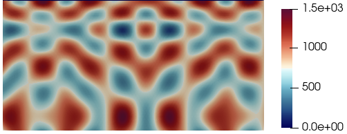
Figure 2. The permeability field in $\Omega^{d}=[0,1]\times[0,0.5]$ defined by eq. 120.

The viscosity is defined by the quarter-power mixing rule as in eq. 119. The other parameters are set as $\mu=0.1$, $\alpha=0.5$, $k_{f}=3$, $h=1/80$, $\Delta t=10^{-3}$, $T=15$, and the source/sink terms are set to zero. In the Darcy region $\Omega^{d}$ the porosity is set to $\phi=0.4$. The dispersion/diffusion tensor is defined as

$$\widetilde{D}(u)=\begin{cases}\delta I,&\text{ in }\Omega^{s},\\ \phi d_{m}\mathbb{I}+d_{l}|u|\mathbb{T}+d_{t}|u|(\mathbb{I}-uu^{T}/|u|^{2}),&\text{ in }\Omega^{d},\end{cases}$$

where $d_{l},d_{t}$, and $d_{m}$ represent longitudinal and transverse dispersivities and the molecular diffusivity, respectively, and $u^{T}$ is the transpose of the vector $u$. Under the condition $d_{l}\geq d_{t}$ (which is usually the case), $D(u)$ satisfies the assumptions eqs. 4a, 4b and 4c (see, for example, [26], [49, Lemmas 4.3, 4.4], and [44, Lemma 1.3]). In this numerical experiment, we choose $\delta=10^{-6}$, $d_{m}=10^{-5}$, $d_{l}=10^{-5}$, and $d_{t}=10^{-5}$. The initial velocity is set to zero while the initial concentration of the plume of contaminant is defined as

$$c_{0}(x)=\begin{cases}0.95&\text{if}\ \sqrt{(x_{1}-0.2)^{2}+(x_{2}-0.7)^{2}}<0.1,\\ 0.05&\text{otherwise}.\end{cases}$$

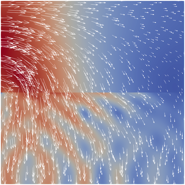
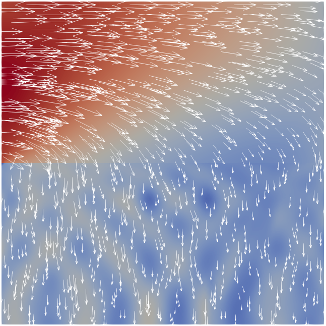
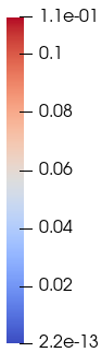
Figure 3. The velocity field after one time step (left) and at the final time (right) for the example in Section 7.3. The color represents the magnitude of the velocity.

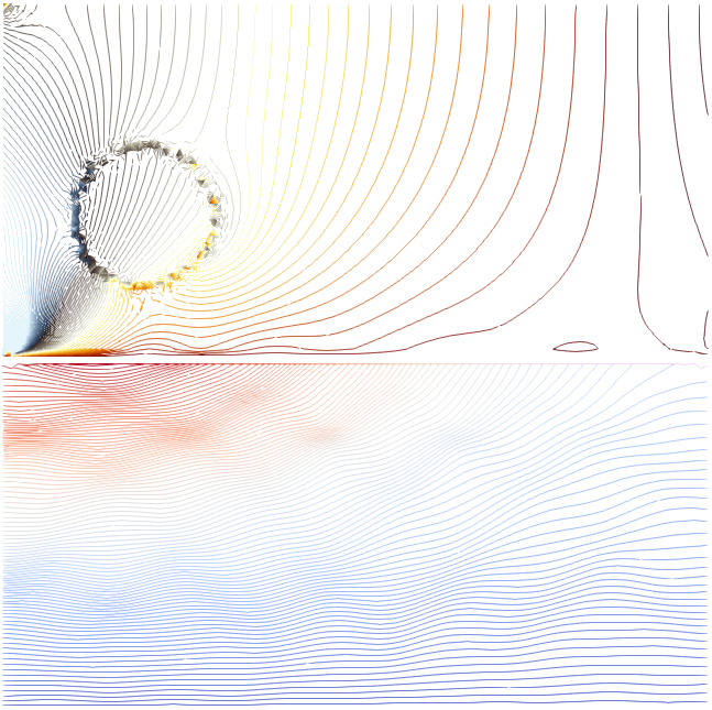
(a) $t=\Delta t$

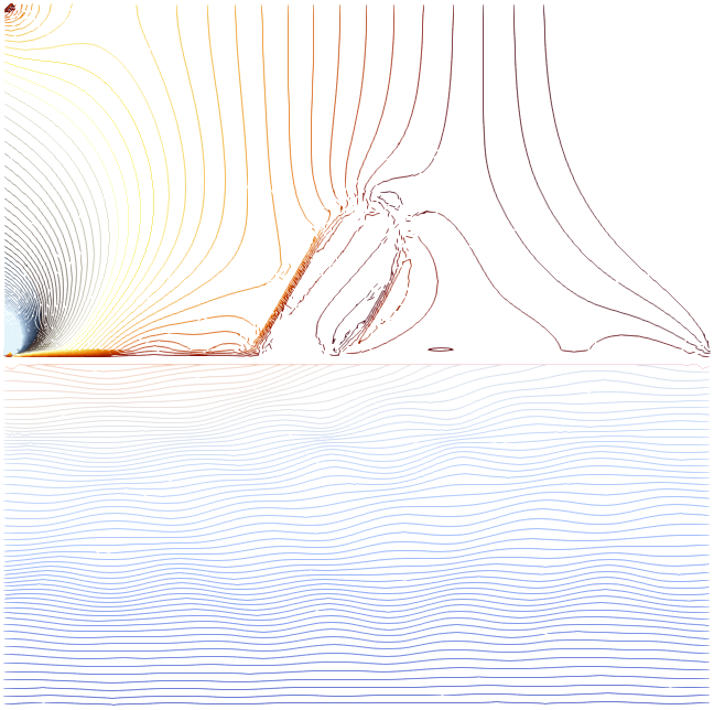
(b) $t=3$

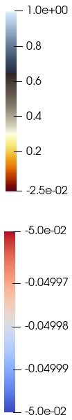
(c)

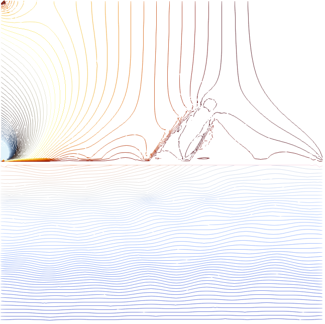
(d) $t=6$

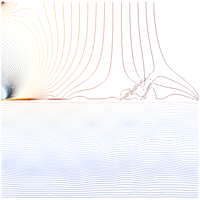
(e) $t=9$

(f)

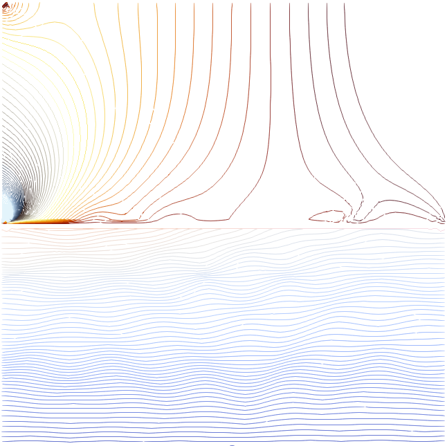
(g) $t=12$.

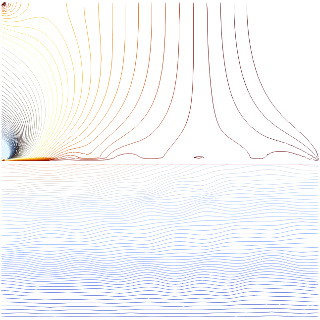
(h) $t=15$

(i)

Figure 4. Pressure contours at times $t=\Delta t,3,6,9,12,15$ for the example in Section 7.3. The color represents the concentration values.

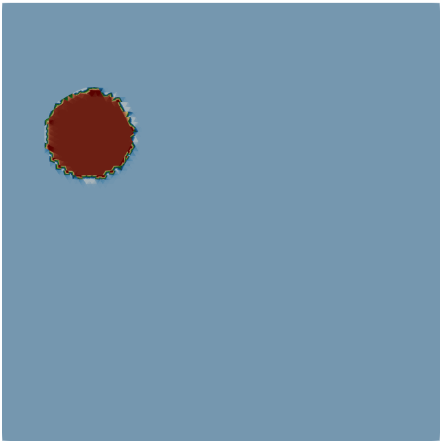
(a) $t=\Delta t$.

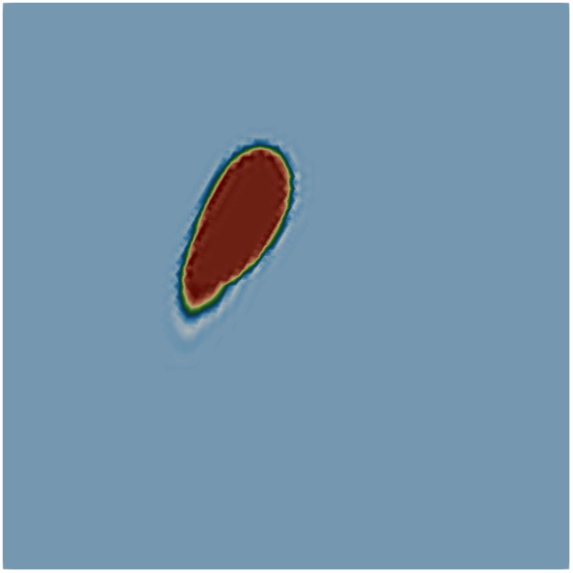
(b) $t=3$.

(c)

(d) $t=6.0$.

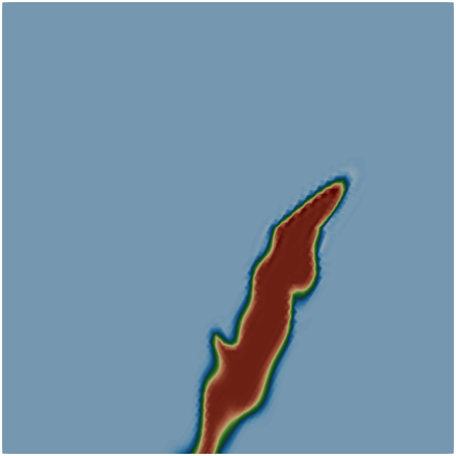
(e) $t=9$.

(f)

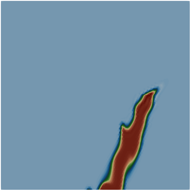
(g) $t=12$.

(h) $t=15$.

(i)

Figure 5. The plume of contaminant at times $t=\Delta t,3,6,9,12,15$ for the example in Section 7.3. The color represents the concentration values.

We compute the solution using BDF3 time stepping. Figure 3 shows the computed velocity field after one time step and at the final time. In the Darcy region $\Omega^{d}$, the flow field avoids areas with low permeability as expected. Figure 4 shows the pressure contours at various times which demonstrates the effect of the concentration on the pressure around the plume of contaminants, especially in the Stokes region. Figure 5 presents the plume of contaminant spreading through the surface water region and infiltrating the porous medium. We plot the solution 6 different instances in time. The contaminant plume stays compact while in the surface water region. Once it reaches the subsurface region it spreads out following a path dictated by the heterogeneous permeability structure of the porous medium.

8. Conclusions

In this paper, we introduced and analyzed a fully discrete sequential method for the fully coupled Stokes/Darcy–transport problem. The spatial discretization uses the HDG method which is higher-order accurate, strongly mass conservative, and compatible. We remark that the analysis also easily extends to the EDG-HDG method considered in [17, 16]. The sequential method discussed in the article linearizes the problem by time-lagging the concentration and decoupling the Stokes/Darcy and transport subproblems. We proved well-posedness and obtained a priori estimates in the energy norm. Finally, we presented numerical results demonstrating mass conservation and robustness with respect to varying permeability and optimal convergence in the $L^{2}$-norm for one-way coupling.

References

- [1] R. Adams. Sobolev spaces. Academic Press, Amsterdam Boston, 2003.
- [2] M. Ainsworth and G. Fu. Fully computable a posteriori error bounds for hybridizable discontinuous Galerkin finite element approximations. J. Sci. Comput., 77:443–466, 2018.
- [3] S. Badia and R. Codina. Unified stabilized finite element formulations for the Stokes and the Darcy problems. SIAM J. Numer. Anal., 47(3):1971–2000, 2009.
- [4] J. Bear and A. H.-D. Cheng. Modeling groundwater flow and contaminant transport, volume 23 of Theory and Applications of Transport in Porous Media. Springer, 2010.
- [5] G. S. Beavers and D. D. Joseph. Boundary conditions at a naturally impermeable wall. J. Fluid. Mech, 30(1):197–207, 1967.
- [6] S. C. Brenner. Poincaré-Friedrichs inequalities for piecewise functions. SIAM J. Numer. Anal., 41(1):306–324, 2003.
- [7] S. C. Brenner. Korn’s inequalities for piecewise vector fields. Math. Comp., 73(247):1067–1087, 2004.
- [8] S. C. Brenner and L. R. Scott. The Mathematical Theory of Finite Element Methods. Springer, 3rd edition, 2010.
- [9] F. Brezzi and M. Fortin. Mixed and Hybrid Finite Element Methods, volume 15 of Springer Series in Computational Mathematics. Springer–Verlag New York Inc., 1991.
- [10] A. N. Brooks and T. J. R. Hughes. Streamline upwind Petrov–Galerkin formulations for convection dominated flows with particular emphasis on the incompressible Navier–Stokes equation. Comput. Meth. Appl. Mech. Engrg., 32(1):199–259, 1982.
- [11] E. Burman and P. Hansbo. Stabilized Crouzeix–Raviart element for the Darcy–Stokes problem. Numer. Meth. Part. D. E., 21(5):986–97, 2005.
- [12] J. Camaño, G. N. Gatica, R. Oyarzúa, R. Ruiz-Baier, and P. Venegas. New fully-mixed finite element methods for the Stokes–Darcy coupling. Comput. Method. Appl. M., 295:362 – 395, 2015.
- [13] Y. Cao, M. Gunzburger, X. Hu, F. Hua, X. Wang, and W. Zhao. Finite element approximations for Stokes–Darcy flow with Beavers–Joseph interface conditions. SIAM J. Numer. Anal., 47(6):4239–4256, 2010.
- [14] A. Çeşmelioğlu and B. Rivière. Existence of a weak solution for the fully coupled Navier–Stokes/Darcy–transport problem. J. Differ. Equations, 252(7):4138–4175, 2012.
- [15] A. Cesmelioglu and P. Chidyagwai. Numerical analysis of the coupling of free fluid with a poroelastic material. Numer Methods Partial Differential Eq., 36:463–494, 2020.
- [16] A. Cesmelioglu and S. Rhebergen. A compatible embedded-hybridized discontinuous Galerkin method for the Stokes–Darcy-transport problem. Commun. Appl. Math. Comput., 2021.
- [17] A. Cesmelioglu, S. Rhebergen, and G. N. Wells. An embedded-hybridized discontinuous Galerkin method for the coupled Stokes–Darcy system. J. Comput. Appl. Math, 367, 2020.
- [18] N. Chaabane, V. Girault, C. Puelz, and B. Riviere. Convergence of IPDG for coupled time-dependent Navier–Stokes and Darcy equations. J. Comput. Appl. Math., 324:25–48, 2017.
- [19] B. Cockburn, J. Gopalakrishnan, and R. Lazarov. Unified hybridization of discontinuous Galerkin, mixed, and continuous Galerkin methods for second order elliptic problems. SIAM J. Numer. Anal., 47(2):1319–1365, 2009.
- [20] B. Cockburn and C.-W. Shu. The local discontinuous Galerkin finite element method for time-dependent convection–diffusion systems. SIAM J. Numer. Anal., 35(6):2440–2463, 1998.
- [21] C. D’Angelo and P. Zunino. Robust numerical approximation of coupled Stokes’ and Darcy’s flows applied to vascular hemodynamics and biochemical transport. ESAIM: M2AN, 45(3):447–476, 2011.
- [22] C. Dawson, S. Sun, and M. F. Wheeler. Compatible algorithms for coupled flow and transport. Comput. Methods Appl. Mech. Engrg., 193:2565–2580, 2004.
- [23] D. A. Di Pietro and A. Ern. Mathematical aspects of discontinuous Galerkin methods, volume 69 of Mathématiques et Applications. Springer–Verlag Berlin Heidelberg, 2012.
- [24] M. Discacciati. Domain decomposition methods for the coupling of surface and groundwater flows. PhD thesis, Ecole Polytechnique Federale de Sausanne, Sausanne, Switzerland, 2004.
- [25] M. Discacciati, E. Miglio, and A. Quarteroni. Mathematical and numerical models for coupling surface and groundwater flows. Appl. Numer. Math., 43(1):57 – 74, 2002. 19th Dundee Biennial Conference on Numerical Analysis.
- [26] J. Douglas Jr., R. E. Ewing, and M. F. Wheeler. A time-discretization procedure for a mixed finite element approximation of miscible displacement in porous media. RAIRO. Anal. numér., 17(3):249–265, 1983.
- [27] A. Ern and J.-L. Guermond. Theory and practice of finite elements, volume 159 of Applied Mathematical Sciences. Springer–Verlag New York, 2004.
- [28] V. Ervin, M. Kubacki, W. Layton, M. Moraiti, Z. Si, and C. Trenchea. Partitioned penalty methods for the transport equation in the evolutionary Stokes–Darcy–transport problem. Numer. Meth. Part. D. E., 35(1):349–374, 2019.
- [29] G. N. Gatica, S. Meddahi, and R. Oyarzúa. A conforming mixed finite-element method for the coupling of fluid flow with porous media flow. IMA J. Numer. Anal., 29:86–108, 2009.
- [30] V. Girault, G. Kanschat, and B. Rivière. Error analysis for a monolithic discretization of coupled Darcy and Stokes problems. J. Numer. Math., 22(2):109–142, 2014.
- [31] V. Girault and B. Rivière. DG approximation of coupled Navier–Stokes and Darcy equations by Beaver–Joseph–Saffman interface condition. SIAM J. Numer. Anal., 47(3):2052–2089, 2009.
- [32] J. Guzmán, C.-W. Shu, and F. Sequeira. H(div) conforming and DG methods for incompressible Euler’s equations. IMA J. Numer. Anal., 37(4):1733–1771, 2016.
- [33] P. Hansbo and M. G. Larson. Discontinuous Galerkin methods for incompressible and nearly incompressible elasticity by Nitsche’s method. Comput. Methods Appl. Mech. Engrg., 191:1895–1908, 2002.
- [34] N. Hanspal, A. Waghode, V. Nassehi, and R. Wakeman. Numerical analysis of coupled stokes/darcy flows in industrial filtrations. Transport in Porous Media, 64(1):1573–1634, 2006.
- [35] G. Kanschat and B. Rivière. A strongly conservative finite element method for the coupling of Stokes and Darcy flow. J. Comput. Phys., 229(17):5933–5943, 2010.
- [36] W. Layton. Introduction to the Numerical Analysis of Incompressible Viscous Flows. Society for Industrial and Applied Mathematics, Philadelphia, PA, 2008.
- [37] W. Layton, F. Schieweck, and I. Yotov. Coupling fluid flow with porous media flow. SIAM J. Numer. Anal., 40(6):2195–2218, 2002.
- [38] J. Lohrenz, B. G. Bray, and C. R. Clark. Calculating viscosities of reservoir fluids from their compositions. J. Petrol. Technol., 16:1171–1176, 1964.
- [39] A. Márquez, S. Meddahi, and F. J. Sayas. Strong coupling of finite element methods for the Stokes–Darcy problem. IMA J. Numer. Anal., 35(2):969–988, 2015.
- [40] N. C. Nguyen, J. Peraire, and B. Cockburn. An implicit high-order hybridizable discontinuous Galerkin method for linear convection-diffusion equations. J. Comput. Phys., 228(9):3232–3254, 2009.
- [41] B. Rivière. Analysis of a discontinuous finite element method for the coupled Stokes and Darcy problems. J. Sci. Comput., 22(1):479–500, 2005.
- [42] B. Rivière. Discontinuous Galerkin methods for solving elliptic and parabolic equations, volume 35 of Frontiers in Applied Mathematics. Society for Industrial and Applied Mathematics (SIAM), Philadelphia, 2008.
- [43] B. Riviere. Discontinuous finite element methods for coupled surface–subsurface flow and transport problems. In X. Feng, O. Karakashian, and Y. Xing, editors, Recent Developments in Discontinuous Galerkin Finite Element Methods for Partial Differential Equations: 2012 John H Barrett Memorial Lectures, pages 259–279. Springer International Publishing, Cham, 2014.
- [44] B. Rivière and N. J. Walkington. Convergence of a discontinuous Galerkin method for the miscible displacement equation under low regularity. SIAM J. NUMER. ANAL., 49(3):1085–1110, 2011.
- [45] H. Rui and J. Zhang. A stabilized mixed finite element method for coupled Stokes and Darcy flows with transport. Comput. Methods Appl. Mech. Engrg., 315:169–189, 2017.
- [46] P. Saffman. On the boundary condition at the surface of a porous media. Stud. Appl. Math., 50:292–315, 1971.
- [47] J. Schöberl. NETGEN an advancing front 2D/3D-mesh generator based on abstract rules. Computing and Visualization in Science, 1:41–52, 1997.
- [48] J. Schöberl. C++11 implementation of finite elements in NGSolve. Technical Report ASC Report 30/2014, Institute for Analysis and Scientific Computing, Vienna University of Technology, 2014.
- [49] S. Sun, B. Rivière, and M. F. Wheeler. A combined mixed finite element and discontinuous Galerkin method for miscible displacement problem in porous media. In Recent Progress in Computational and Applied PDES, pages 323–351, Boston, MA, 2002. Springer US.
- [50] S. Sun and M. F. Wheeler. Discontinuous Galerkin methods for coupled flow and reactive transport problems. Applied Numerical Mathematics, 52(2):273–298, 2005.
- [51] D. Vassilev and I. Yotov. Coupling Stokes–Darcy flow with transport. SIAM J. Sci. Comput., 31(5):3661–3684, 2009.
- [52] G. N. Wells. Analysis of an interface stabilized finite element method: the advection-diffusion-reaction equation. SIAM J. Numer. Anal., 49(1):87–109, 2011.