Long Dark Gaps in the Ly$\beta$ Forest at $z<6$: Evidence of Ultra Late Reionization from XQR-30 Spectra

Abstract

We present a new investigation of the intergalactic medium (IGM) near reionization using dark gaps in the Lyman-$\beta$ (Ly${\beta}$) forest. With its lower optical depth, Ly${\beta}$ offers a potentially more sensitive probe to any remaining neutral gas compared to commonly used Ly$\alpha$ line. We identify dark gaps in the Ly${\beta}$ forest using spectra of 42 QSOs at $z_{\rm em}>5.5$, including new data from the XQR-30 VLT Large Programme. Approximately 40% of these QSO spectra exhibit dark gaps longer than $10{h^{-1}{\rm Mpc}}$ at $z\simeq 5.8$. By comparing the results to predictions from simulations, we find that the data are broadly consistent both with models where fluctuations in the Ly$\alpha$ forest are caused solely by ionizing ultraviolet background (UVB) fluctuations and with models that include large neutral hydrogen patches at $z<6$ due to a late end to reionization. Of particular interest is a very long ($L=28{h^{-1}{\rm Mpc}}$) and dark ($\tau_{\rm eff}\gtrsim 6$) gap persisting down to $z\simeq 5.5$ in the Ly${\beta}$ forest of the $z=5.85$ QSO PSO J025$-$11. This gap may support late reionization models with a volume-weighted average neutral hydrogen fraction of $\langle x_{\rm HI}\rangle\gtrsim 5\%$ by $z=5.6$. Finally, we infer constraints on $\langle x_{\rm HI}\rangle$ over $5.5\lesssim z\lesssim 6.0$ based on the observed Ly${\beta}$ dark gap length distribution and a conservative relationship between gap length and neutral fraction derived from simulations. We find $\langle x_{\rm HI}\rangle\leq 0.05$, 0.17, and 0.29 at $z\simeq 5.55$, 5.75, and 5.95, respectively. These constraints are consistent with models where reionization ends significantly later than $z=6$.

1 Introduction

Determining when and how reionization occurred is essential for understanding the IGM physics and galaxy formation in the early Universe (e.g., Muñoz et al., 2022). Recent observations have made significant progress on establishing the timing of reionization and largely point to a midpoint of $z\sim 7-8$. These observations include the electron optical depth to the cosmic microwave background (CMB) photons (Planck Collaboration et al., 2020, see also de Belsunce et al., 2021), the Lyman-$\alpha$ (Ly$\alpha$) damping wing in $z\gtrsim 7$ QSO spectra (e.g., Bañados et al., 2018; Davies et al., 2018b; Wang et al., 2020; Yang et al., 2020a; Greig et al., 2021), the decline in observed Ly$\alpha$ emission from $z>6$ galaxies (e.g., Mason et al., 2018, 2019; Hoag et al., 2019; Hu et al., 2019, and references therein, but see Jung et al., 2020; Wold et al., 2021), and the IGM thermal state measurements at $z>5$ (e.g., Boera et al., 2019; Gaikwad et al., 2021).

The observations noted above are generally consistent with reionization ending by $z\sim 6$, a scenario supported by existing measurement of the fraction of dark pixels in the Lyman series forests (e.g., McGreer et al., 2011, 2015). Other observations, however, suggest a significantly later end of reionization. The large-scale fluctuations in the measured Ly$\alpha$ effective optical depth, $\tau_{\rm eff}=-\ln{\langle F\rangle}$, where $F$ is the continuum-normalized transmission flux (e.g., Fan et al., 2006; Becker et al., 2015; Eilers et al., 2018; Bosman et al., 2021b; Yang et al., 2020b), together with long troughs extending to or below $z\simeq 5.5$ in the Ly$\alpha$ forest (e.g., Becker et al., 2015; Zhu et al., 2021) potentially indicate the existence of large neutral IGM islands (e.g., Kulkarni et al., 2019; Keating et al., 2020b; Nasir & D’Aloisio, 2020). The underdensities around long dark gaps traced by Ly$\alpha$ emitting galaxies (LAEs) are also consistent with a late reionization model wherein reionization ends at $z<6$ (Becker et al., 2018; Kashino et al., 2020; Christenson et al., 2021).

These Ly$\alpha$ forest and LAE results are potentially consistent with an alternative scenario wherein the IGM is ionized by $z=6$ but retains large-scale fluctuations in the ionizing UV background down to lower redshifts (Davies et al., 2018a). On the other hand, recent measurements of the mean free path of ionizing photons measured at $z=5.1$ and 6.0 (Becker et al., 2021) are difficult to reconcile with models wherein reionization ends at $z>6$, and may instead prefer models wherein the IGM is still $20\%$ neutral or more at $z=6$ (Becker et al., 2021; Cain et al., 2021; Davies et al., 2021). In addition, a reionization ending at $z<6$ is consistent with models that reproduce a variety of observations (e.g., Weinberger et al., 2019; Choudhury et al., 2021; Qin et al., 2021).

One way of searching for signatures of late ($z_{\rm end}<6$) reionization in the Ly$\alpha$ forest is by investigating dark gaps, i.e., contiguous regions of strong absorption (e.g., Songaila & Cowie, 2002; Furlanetto et al., 2004; Paschos & Norman, 2005; Fan et al., 2006; Gallerani et al., 2008; Gnedin et al., 2017; Nasir & D’Aloisio, 2020). In Zhu et al. (2021, hereafter Paper I), we explored long dark gaps in the Ly$\alpha$ forest and found that a fully ionized IGM with a homogeneous UVB is strongly ruled out down to $z\simeq 5.3$. In contrast, late reionization models and a model wherein reionization ends by $z\sim 6$ but retains large-scale UVB fluctuations are consistent with the observations. Predictions for the Ly$\alpha$ dark gap statistics are similar between the two types of models. This is largely because realistic late reionization models also include UVB fluctuations, which are often associated with the neutral islands. Ly$\alpha$ also tends to saturate at a relatively low ($x_{\rm HI}\sim 10^{-3}$) neutral fraction, limiting its sensitivity to neutral gas.

Given its lower optical depth , Ly${\beta}$ should be a more sensitive probe of neutral gas in the $z\lesssim 6$ IGM. As a result, ultra-late reionization models wherein neutral islands persist down to $z<5.5$ may produce more long Ly${\beta}$ dark gaps than can be produced by UVB fluctuations alone. Based on this feature, we can potentially use dark gaps in the Ly${\beta}$ forest to place stronger constraints on the timing of reionization and distinguish the late reionization models from the pure fluctuating UVB models. As presented in Nasir & D’Aloisio (2020), distributions of dark gaps in the Ly${\beta}$ forest differ between these models most strongly on scales of $L\gtrsim 10{h^{-1}{\rm Mpc}}$. We are therefore particularly interested in these long dark gaps.

In this work, we use 42 high-quality QSO spectra that allow us to search for dark gaps in the Ly${\beta}$ forest over the redshift range $5.5<z<6.0$. The sample includes high-quality X-Shooter spectra from the XQR-30 VLT large program (D’Odorico et al., in prep.). In addition to comparing the results to model predictions, we also constrain $\langle x_{\rm HI}\rangle$ based on a conservative relationship between dark gap length and neutral fraction derived from simulations.

This paper is organized as follows. In Section 2 we describe the data and results from the observations. Section 3 compares our results to model predictions, discusses the implications for reionization, and infers constraints on $x_{\rm HI}$. Finally, we conclude the findings in Section 4. Throughout this paper, we assume a $\Lambda$CDM cosmology with $\Omega_{\rm m}=0.308$, $\Omega_{\Lambda}=0.692$, and $h=0.678$ (Planck Collaboration et al., 2014). Distances are quoted in comoving units unless otherwise noted.

2 The Data and Results

2.1 QSO Spectra

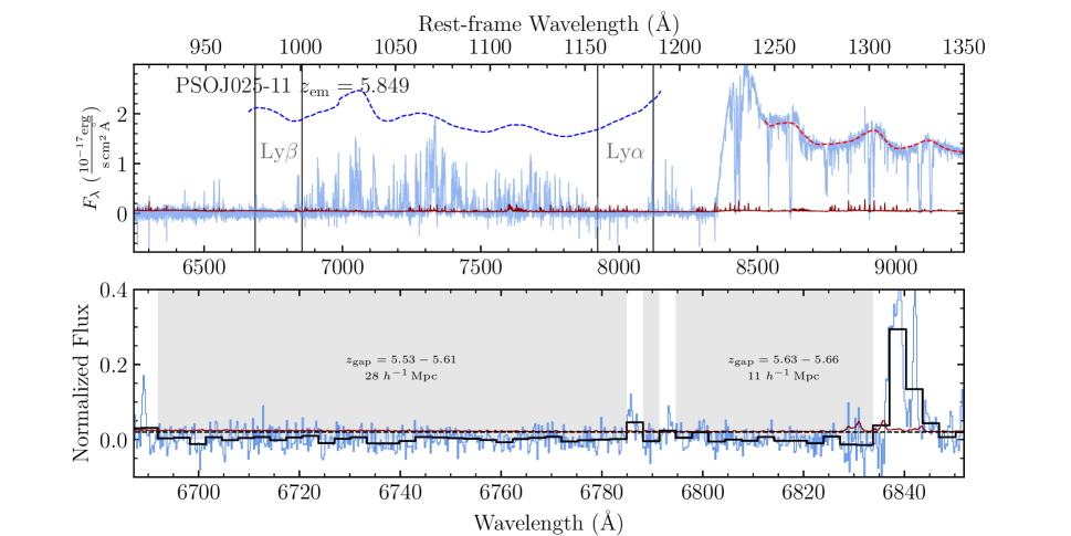
Figure 1: Top panel: Spectrum and continuum fits for the $z_{\rm em}=5.849$ QSO PSO J025$-$11. The light blue and dark red lines represents flux and flux error in the original binning. Dashed curves redward and blueward of the Ly$\alpha$ peak show the best-fitting and predicted QSO continuum in absence of absorption, respectively. The fitting and prediction are based on Principal Component Analysis (PCA). The continuity between the Ly$\alpha$ forest and the Ly${\beta}$ forest continuum is broken intentionally near 1020 Å in the rest frame. We label the wavelength range over which we search for dark gaps in the Ly${\beta}$ forest and its corresponding Ly$\alpha$ forest in redshift. Bottom panel: Ly${\beta}$ forest and dark gaps detected. The dashed black line labels the flux threshold of 0.02. The thick black line displays the flux binned to $1{h^{-1}{\rm Mpc}}$. Light blue and dark red lines show the flux and flux error in the original binning. Dark gaps detected are shaded with gray. We also label the redshift range and length of each long ($L\geq 10{h^{-1}{\rm Mpc}}$) dark gap.
(The complete figure set [42 images] is available online at https://ydzhuastro.github.io/lyb.html.)

Our sample includes the 42 out of 43 spectra of QSOs at $5.77\lesssim z_{\rm em}\lesssim 6.31$ that were used for Paper I. The exception is PSO J004$+$17, whose spectrum has lower S/N that does not meet the requirement of our flux threshold for the Ly${\beta}$ forest (Section 2.3). The spectra are taken with the Echellette Spectrograph and Imager (ESI) on Keck (Sheinis et al., 2002) and the X-Shooter spectrograph on the Very Large Telescope (VLT; Vernet et al., 2011). Among these, 19 X-Shooter spectra are from the XQR-30 VLT large program (D’Odorico et al., in prep). The details of the data reduction procedures are given in Paper I and Becker et al. (2019). We note that the targets are selected without foreknowledge of dark gaps in the Ly${\beta}$ forest. Figure Set 1 displays the spectra, continuum fits, and dark gaps detected in the Ly${\beta}$ forest for each QSO (see details below). An example is given in Figure 1.

2.2 Continuum Fitting

We use Principal Component Analysis (PCA) to predict the unabsorbed QSO continuum and normalize the transmission in the Ly${\beta}$ forest. We follow a similar method as described in Paper I to fit and predict the continuum. Briefly, we implement and apply the log-PCA method of Davies et al. (2018c) in the Ly$\alpha$ and Ly${\beta}$ forest portion of the spectrum following Bosman et al. (2021b). The continuity between the Ly$\alpha$ forest and the Ly${\beta}$ forest continuum is broken intentionally to correct for the effect of overlapping Ly$\alpha$ absorption in the Ly${\beta}$ forest in the PCA training sample. We fit the red-side (rest-frame wavelength $\lambda_{0}>1230$ Å) continuum up to 2000 Å in the rest frame for X-Shooter spectra with NIR observations. The ESI spectra are fit using an optical-only PCA, which is presented in Bosman et al. (2021a). The Ly${\beta}$ dark gap detection is not very sensitive to the continuum, and we also test that using a power-law continuum does not significantly change the dark gap results in this work.

2.3 Dark Gap Detection

Similar to the definition of a dark gap in the Ly$\alpha$ forest in Paper I, we define a dark gap in the Ly${\beta}$ forest to be a continuous spectral region in which all pixels binned to $1{h^{-1}{\rm Mpc}}$ have an observed normalized flux $F=F_{\rm obs}/F_{\rm c}<0.02$, where $F_{\rm obs}$ is the observed flux and $F_{\rm c}$ is the continuum flux. The minimum length of a dark gap is $1{h^{-1}{\rm Mpc}}$ following Paper I. A bin size of $1{h^{-1}{\rm Mpc}}$ enables us to retain significant transmission profiles while reducing the influence of very small peaks on dark gap detection. The precise bin size should have relatively little impact on our results provided that the observations and mock spectra are treated consistently. We have verified that using bin sizes of $0.5{h^{-1}{\rm Mpc}}$ or $1.5{h^{-1}{\rm Mpc}}$ does not change our major conclusions, although the lengths of some dark gaps would change. A flux threshold of 0.02 is used here instead of 0.05, which we used for the Ly$\alpha$ gaps, because spectra in this sub-sample have higher signal-to-noise (S/N) levels. In addition, the Ly${\beta}$ forest at the redshifts that we are interested in is less contaminated by sky lines than the Ly$\alpha$ forest. We have tested that using a threshold of 0.05 will not change our results fundamentally, although the difference between the models (Section 3) may become less significant. In order to reduce false detections caused by foreground Ly$\alpha$ absorption, we further require that all Ly${\beta}$ dark gaps correspond to Ly$\alpha$ dark gaps as defined in Paper I over the same redshifts for both the observed and mock (Section 3.1) spectra. That is to say, each $1{h^{-1}{\rm Mpc}}$ bin in the Ly${\beta}$ dark gap also has a normalized flux less than 0.05 in the Ly$\alpha$ forest at the same redshift. For reference, we present the relationship between Ly${\beta}$ dark gaps and Ly$\alpha$ dark gaps in Appendix A.

For each QSO sightline, dark gaps are detected from 976 Å in the rest frame to 11 proper-Mpc blueward of the QSO’s redshift, which corresponds to approximately 1000 Å in the rest frame. The lower wavelength limit ensures that the detection is not affected by the Ly$\gamma$ absorption. We use the higher limit to avoid the QSO proximity zone transmission, and the cut is comparable to the choice in, e.g., Bosman et al. (2021a). Following Paper I, we also exclude from the statistical analysis an additional $10{h^{-1}{\rm Mpc}}$ buffer zone blueward of the proximity zone cut. This allows the pixel at the red end of each sightline to intersect a possible long ($L\geq 10{h^{-1}{\rm Mpc}}$) dark gap, and hence helps to mitigate potential truncation issues.

To avoid the contamination from sky line subtraction residuals, we mask out $\pm 75~{}{\rm km\,s^{-1}}$ intervals of the spectra centered at sharp peaks in the flux error array when searching for dark gaps. The exception is that we do not mask transmission with a $>3\sigma$ detection. In addition, we make no attempts to correct for the effects of damped Ly$\alpha$ systems (DLAs) or metal-enriched absorbers, although known systems in a sub-sample of the spectra with a relatively complete identification of metal-enriched systems are discussed in Appendix B. Figure 2 displays an overview of dark gaps detected in the Ly${\beta}$ forest from our sample.

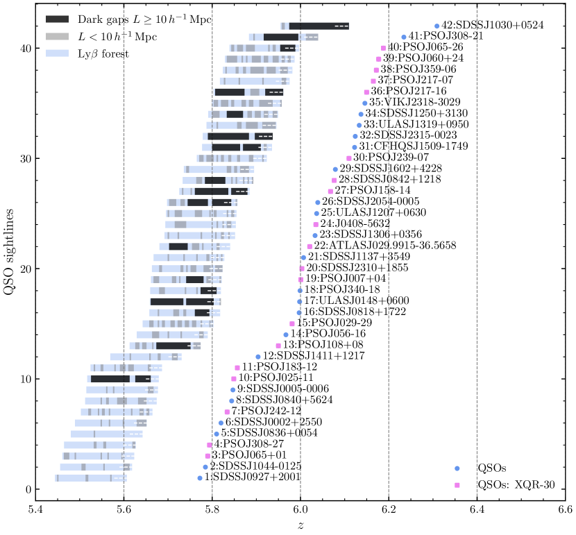
Figure 2: Overview of dark gaps identified in the Ly${\beta}$ forest from our sample of 42 QSO spectra. Black (gray) bars represent dark gaps longer (shorter) than $10{h^{-1}{\rm Mpc}}$. Pink squares label redshifts of XQR-30 targets, and blue dots mark the redshifts of the rest of QSOs. Light blue shaded regions demonstrate the redshift coverage of the Ly${\beta}$ forest. We note that the Ly${\beta}$ forest is truncated at 11 pMpc from the QSO. The Ly${\beta}$ forest shown in this figure includes the $10{h^{-1}{\rm Mpc}}$ buffer zone labeled with dashed white line at the red end.

2.3.1 Dark Gaps Statistics

Figure 3: Observed Ly${\beta}$ dark gaps. (a) Gap length versus central redshift. Dark gaps cut at the red end by the proximity zone cut are labeled with arrows. (b) Cumulative distribution of dark gap length for two redshift intervals. The upper/lower bounds of the shaded region are described in Section 2.3.1. (c) The fraction of QSO spectra showing dark gaps longer than $10{h^{-1}{\rm Mpc}}$ as a function of redshift, $F_{10}$. $F_{10}$ is plotted with a binning of $\Delta z=0.025$. See text and Appendix C for discussions about the drop of $F_{10}$ near $z=5.9$.
(The data used to create this figure are available online at https://ydzhuastro.github.io/lyb.html.)

Figure 3 displays the statistical properties of dark gaps detected in the Ly${\beta}$ forest from our sample. We detect 195 dark gaps in total, of which 24 have $L\geq 10{h^{-1}{\rm Mpc}}$. Panel (a) plots length versus central redshift of these dark gaps. Long dark gaps become less common as redshift decreases. Nevertheless, some long gaps still exist down to $z<5.6$.

We calculate the cumulative distribution function of dark gap length, $P(<L)$. Dark gaps are sorted into two redshift bins according to their redshifts at both ends. For distributions that include dark gaps cut at the red end by the proximity zone limit, we calculate a lower bound on $P(<L)$ by assuming a infinite length for these gaps, and an upper bound by assuming the gap length that would appear in the absence of any proximity effect is the same as the one measured. As shown in Figure 3 (b), longer dark gaps become more numerous over $5.75<z<6.00$ compared to $5.50<z<5.75$. This significant evolution of $P(<L)$ is consistent with the results shown in panel (a).

Following Paper I, we quantify the spatial coverage of large Ly${\beta}$-opaque regions by calculating the fraction of QSO spectra showing long ($L\geq 10{h^{-1}{\rm Mpc}}$) dark gaps as a function of redshift, $F_{10}(z)$. Here we use $10{h^{-1}{\rm Mpc}}$ as the threshold because dark gaps longer than this in the late reionization models (see Section 3) are dominated by those containing neutral islands. Based on our tests, the number of dark gaps predicted by different models differs the most for $L\gtrsim 10{h^{-1}{\rm Mpc}}$, as also suggested by Nasir & D’Aloisio (2020).

We calculate $F_{10}$ at each redshift and average over $\Delta z=0.025$ bins. As shown in Figure 3 (c), $F_{10}$ has a significant redshift evolution over $5.5<z<6.0$. It increases rapidly with redshift over $5.5<z<5.8$, from $\sim 10\%$ to $\sim 40\%$, and climbs up to $\sim 80\%$ by $z=6.0$ after a drop at $z\sim 5.9$. The reason of the drop is unclear, but the limited number of QSO sightlines may produce large statistical fluctuations (Appendix C), as also shown in the model predictions in Section 3. For comparison, we compute $F_{01}$, the fraction of QSO sightlines exhibiting dark gaps with $L\geq 1{h^{-1}{\rm Mpc}}$, and find no significant drop near $z=5.9$ (see Appendix C).

2.3.2 Long Dark Gap toward PSO J025$-$11

We find a particularly interesting Ly${\beta}$ gap toward the $z=5.849$ QSO PSO J025$-$11 (Figure 1). This dark gap is within the redshift interval of a long ($68{h^{-1}{\rm Mpc}}$) trough in the Ly$\alpha$ forest. It spans $5.526\leq z\leq 5.613$ with a length of $28{h^{-1}{\rm Mpc}}$. This is longer and extending to a even lower redshift than the 19 and $23{h^{-1}{\rm Mpc}}$ Ly${\beta}$ troughs with $z_{\rm min}=5.66$ within the extreme ($110{h^{-1}{\rm Mpc}}$) Ly$\alpha$ trough over $5.523\leq z\leq 5.879$ toward ULAS J0148$+$0600 (Becker et al., 2015). This dark gap toward J025$-$11 contains no apparent transmission peaks, even in the unbinned data. The $2\sigma$ lower limit of $\tau_{\rm eff}\geq 6.067$ measured over the complete trough indicates that it is highly opaque.

There is a possibility that part of the trough may be due to either Ly${\beta}$ or foreground Ly$\alpha$ absorption from the circum-galacitc medium (CGM) around intervening galaxies. In this case, corresponding metal lines may be present. We check for potential CGM absorption using the XQR-30 metal absorber catalog (Davies et al., in prep; see Appendix B for technique details). We find no intervening metal systems within the redshift range of the gap. We note that this line of sight has a DLA near the redshift of the QSO, as evidenced by the damping wing at the blue edge of the Ly$\alpha$ proximity zone. The Ly${\beta}$ gap described here is at a velocity separation of $>$3000$~{}{\rm km\,s^{-1}}$ from the QSO, however, and is unaffected by the DLA. The XQR-30 catalog does include a C IV system towards J025$-$11 at $z=4.5138$, for which Ly$\alpha$ would fall at the blue end of the Ly${\beta}$ trough. Overall, however, the general lack of metal absorbers associated with this long dark gap may suggest that the gap probes a low-density region. This would favor the association of highly opaque sightlines with galaxy underdensities, as seen in imaging surveys for galaxies surrounding long Ly$\alpha$ troughs (Becker et al., 2018; Kashino et al., 2020; Christenson et al., 2021).

We examine the possible role of metal-enriched absorbers more broadly in Appendix B, finding little evidence for a strong correlation with long Ly${\beta}$ troughs. We also examined a sample of lower-redshift lines of sight in Appendix D, finding that metal-enriched absorbers in the foreground Ly$\alpha$ alone are unlikely to create such a long dark gap. We emphasize that this gap falls in redshift within a long Ly$\alpha$ trough spanning $5.461\leq z\leq 5.674$ with $L=68{h^{-1}{\rm Mpc}}$ that does not appear to be affected by metal absorbers (Paper I). This combination of factors gives us confidence that the $L=28{h^{-1}{\rm Mpc}}$ dark gap is genuinely caused by IGM opacity .

3 Models and Discussion

3.1 Models and Mock Spectra

Here we compare our results to predictions from models based on hydrodynamical simulations. We use the following models, which were also used in Paper I:

1. the homogeneous-UVB model from the Sherwood Simulation Suite (Bolton et al., 2017), which uses a homogeneous Haardt & Madau (2012) UV background;

2. late reionization models wherein reionization ends at $z\lesssim 5.3$, including K20-low-$\tau_{\rm CMB}$, K20-low-$\tau_{\rm CMB}$-hot, K20-high-$\tau_{\rm CMB}$ models from Keating et al. (2020a), and ND20-late-longmfp, ND20-late-shortmfp models from Nasir & D’Aloisio (2020); and

3. an early reionization model wherein the IGM is mostly ionized by $z=6$ but large scale fluctuations in the UVB, which are amplified by a short mean free path of ionizing photons ($\lambda_{\rm mfp}^{912}=10{h^{-1}{\rm Mpc}}$ at $z=5.6$), persist down to lower redshifts (ND20-early-shortmfp, Nasir & D’Aloisio, 2020).

These models were chosen, in part, because they reproduce at least some other observations of the Ly$\alpha$ forest. The homogeneous-UVB model agrees well with observations at $z<5$ including the IGM temperature and flux power spectra (Bolton et al., 2017), although it fails to predict the Ly$\alpha$ opacity distribution at $z>5$ (e.g., Bosman et al., 2021b). The late reionization and fluctuating UVB models are broadly consistent with observations of IGM temperature, mean Ly$\alpha$ transmission, and fluctuations in Ly$\alpha$ opacity over the redshift range we are interested in (Keating et al., 2020a; Nasir & D’Aloisio, 2020). Moreover, these models are able to produce long Ly$\alpha$ troughs at $z<6$ (e.g., Paper I). We note that, nevertheless, that none of the models we use can self-consistently predict the mean free path evolution over $5<z<6$ as measured in Becker et al. (2021).

In the homogeneous-UVB model, the IGM is instantaneously reionized at $z=15$. At $z<6$, therefore, the IGM in this model is fully ionized and the gas is hydrodynamically relaxed. A homogeneous UVB model that produced a later reionization (e.g., Puchwein et al., 2019; Villasenor et al., 2021) would mainly alter the temperature and pressure smoothing at $z<6$. These are small-scale effects, however, that should only minimally impact our measurements. We would generally expect that any homogeneous UVB model that reionizes by $z=6$ would produce similar dark gap statistics as the Haardt & Madau (2012) UVB once the ionization rates at $z<6$ are rescaled to reproduce the observed mean flux.

The K20-low-$\tau_{\rm CMB}$-hot model shares a similar reionization history with the K20-low-$\tau_{\rm CMB}$ model, but it has a different thermal history with a volume-weighted mean temperature at the mean density at $z=6$ of $T_{0}=10,000$ K compared to that of the latter being 7000 K. The K20-high-$\tau_{\rm CMB}$ model has an earlier mid-point of reionization at $z=8.4$, which is at the upper end of the value suggested by CMB measurements (Planck Collaboration et al., 2020). As for the late reionization models from Nasir & D’Aloisio (2020), the main difference is that the ND20-late-shortmfp model includes stronger post-reionization UVB fluctuations than the ND20-late-longmfp model, while they both have neutral islands surviving at $z<6$. The mean free path of ionizing photons at $z=5.6$ in these two models are $\lambda_{\rm mfp}^{912}=10$ and 30 ${h^{-1}{\rm Mpc}}$, respectively.

The box sizes we use in this work are $L=160$, 160, and 200 ${h^{-1}{\rm Mpc}}$, for simulations in Bolton et al. (2017), Keating et al. (2020a), and Nasir & D’Aloisio (2020), respectively. We note that the K20 models are from radiative transfer simulations run in post-processing and that the ND20 models are semi-numeric models. For more details on the models, see Paper I.

We rescale the optical depths in the simulations as needed in order to match the observed mean flux in the Ly$\alpha$ forest (see, e.g., §2.2 in Bolton et al., 2017, and references therein). We scale to the measurements of Bosman et al. (2018), which are consistent with the mean Ly$\alpha$ fluxes obtained from our sample. The same rescaling factor is then applied to both the Ly$\alpha$ and corresponding Ly${\beta}$ optical depths. We note that this rescaling mainly applies to the homogeneous-UVB model, for which scaling by factors of $\sim$0.4$-$0.6 is required over $5<z<6$. We are therefore explicitly testing only a homogeneous-UVB model that also matches the observed mean Ly$\alpha$ flux. The Keating et al. (2020a) models already produce a mean Ly$\alpha$ transmission consistent with the measurements of Bosman et al. (2018). The mock spectra from this simulation are continuous in redshift, with a smoothly evolving mean flux. Nasir & D’Aloisio (2020) also calibrated their simulations to the observed $\tau_{\rm eff}$ from Bosman et al. (2018) but provide one-dimensional skewers at discrete redshifts. For these simulations we therefore only need to rescale the optical depths such that the mock spectra described below have a mean flux that evolves smoothly with redshift.

We derive dark gap predictions from forward-modeled mock spectra that are matched to the observed sample in QSO redshift, resolution, and S/N. Keating et al. (2020a) provide mock spectra of the Ly${\beta}$ forest including the foreground Ly$\alpha$ absorption. For the homogeneous-UVB model and models from Nasir & D’Aloisio (2020) we follow the methods described in Paper I to build the mock Ly${\beta}$ forest and foreground Ly$\alpha$ forest. In all cases we re-bin the mock spectra and apply the noise arrays according to each observed spectrum.

3.2 Model Comparisons

3.2.1 Comparisons of $F_{10}$

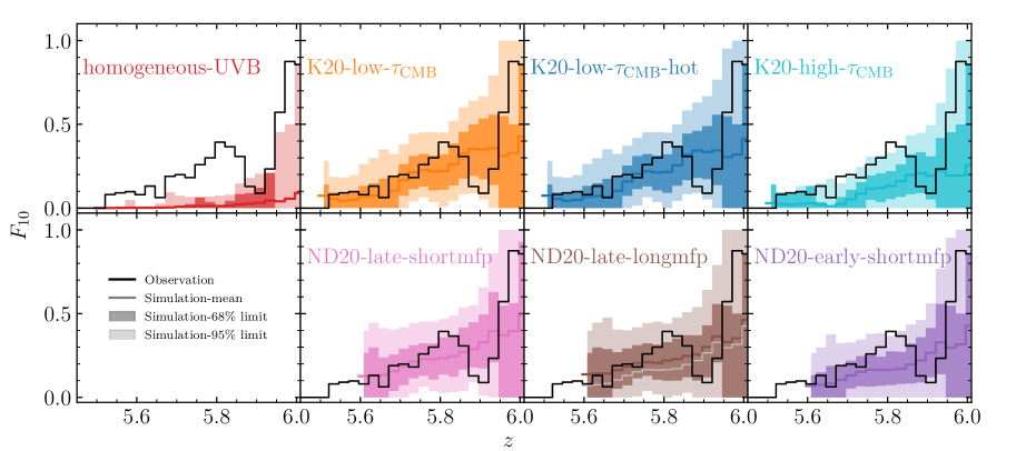
Figure 4: Fraction of QSO spectra showing long ($L\geq 10{h^{-1}{\rm Mpc}}$) Ly${\beta}$ dark gaps as a function of redshift predicted by different models. The colored lines, dark-shaded regions, and light-shaded regions show the mean, 68%, and 95% limits of $F_{10}$ predicted by models based on 10,000 realizations. The black lines plot $F_{10}$ from the observations. For comparison, we also overplot the mean $F_{10}$ predicted by the ND20-early-shortmfp in the panel of the ND20-late-longmfp model with a gray line.

We compute the predicted $F_{10}$ of each model based on 10,000 randomly selected sets of mock spectra of the same size as the observed sample. Their mean, 68%, and 95 % limits are plotted in Figure 4, along with the observations. Similar to $F_{30}$ for the Ly$\alpha$ forest in Paper I, $F_{10}$ shows jagged features due to the combined effects of step changes in the number of sightlines with redshift and the quantization of $F_{10}$ for a finite sample size. We note that 68 and 95 percentile limits can share their upper and/or lower bounds at some redshifts, for the same reason. These features, on the other hand, show the constraining ability of the current sample size and data quality. The drop at $z\sim 5.9$ seen in the observed $F_{10}$ is also broadly included in the 95% limits for most of the models.

The homogeneous-UVB model is not supported by the data at the $\geq 95\%$ level. This is consistent with the conclusion based on the Ly$\alpha$ forest in Paper I that a fully ionized IGM with a homogeneous UVB scenario is disfavored by the data at $z<6$ down to $z\simeq 5.3$. In contrast, the late reionization models are still consistent with the data, except for the K20-high-$\tau_{\rm CMB}$ model, which covers the observed $F_{10}$ just within its 95% upper limit. This supports the conclusion of Paper I that this extended reionization model is less favored by the data due to its insufficient neutral hydrogen and/or UVB fluctuations at $z<6$.

Our results further show that dark gaps in Ly${\beta}$ are more sensitive probes of neutral regions than gaps in Ly$\alpha$. For dark gaps in the Ly$\alpha$ forest, we see little difference between the ND20-early-shortmfp model and the ND20-late models (Paper I). In the Ly${\beta}$ forest, however, the former predicts a smaller $F_{10}$ than the latter by $\sim 0.05$ at most redshifts. This difference is not enough for us to distinguish them based on the current sample, although the Ly${\beta}$ gaps put some pressure on the early reionization model. Nasir & D’Aloisio (2020) note that these models are different in their Ly${\beta}$ dark gap length distributions while they cannot be distinguished in the Ly$\alpha$ forest. Nevertheless, we compute the differential dark gap length distribution for individual $\Delta L$ bins, $L\Delta P(L)/\Delta L$, and find their differences are minor compared to the scatter of the data. Looking ahead to the era of ELTs, we forecast that $\sim 100$ lines of sight with the Ly${\beta}$ forest covering $z\sim 5.8$ would be needed to distinguish the two models at $\sim$95% confidence based on $F_{10}$. A signal-to-noise ratio of 50 per $10\,\rm km\,s^{-1}$ for the spectra would be adequate according to our tests using mock spectra.

3.2.2 Total Number of Long Dark Gaps at $z\leq 5.8$

Figure 5: (a) Number of long ($L\geq 10{h^{-1}{\rm Mpc}}$) Ly${\beta}$ dark gaps that lie entirely below $z=5.8$ in the mock sample from each model. (b) Number of long dark gaps entirely over $5.6\leq z\leq 5.8$. In both panels the center lines, boxes, and error bars show the mean, 68% limits, and 95% limits, respectively. The observed numbers of long dark gaps in each redshift range are indicated by dashed green lines.

To further illustrate the differences between models, we use our mock data to calculate the total number of long dark gaps predicted to lie entirely at $z<5.8$. Figure 5 compares the model results to the observations. Given that the ND20 models only have outputs down to $z=5.6$, we exclude these models when counting the total number of long dark gaps below $z=5.8$. We nevertheless include the ND20 models for dark gaps that fall entirely over $5.6\leq z\leq 5.8$ for reference.

The results are consistent with those from $F_{10}$. As shown in Figure 5 (a), the 95% upper limit of the predicted number of long dark gaps by the homogeneous-UVB model is 2. This is a factor of 4 smaller than the observed value, which is 8. The K20-high-$\tau_{\rm CMB}$ model is also disfavored by the data at $>95\%$ confidence given its deficit of long dark gaps. In contrast, the rapid late reionization models, i.e. K20-low-$\tau_{\rm CMB}$ models, agree with the observations within their $95\%$ limits.

Over $5.6\leq z\leq 5.8$ the observed number of long dark gaps decreases by one while the simulation predictions have little change. In this case, rapid late reionization models from Keating et al. (2020a) are still consistent with the data. The observations also support both fluctuating UVB and late reionization models from Nasir & D’Aloisio (2020). We note that the difference between the predicted mean numbers and the observed value is smallest for the ND20-late models, wherein $\langle x_{\rm HI}\rangle$ is still higher than $\sim 5\%$ by $z=5.6$. On the other hand, the K20-high-$\tau_{\rm CMB}$ model is disfavored by the data also in this redshift range. This would suggest that very extended reionization scenarios in which insufficient neutral hydrogen and/or UVB fluctuations remain at $z<6$ may be disfavored.

3.2.3 Detection Rate of an $L\geq 28{h^{-1}{\rm Mpc}}$ Dark Gap

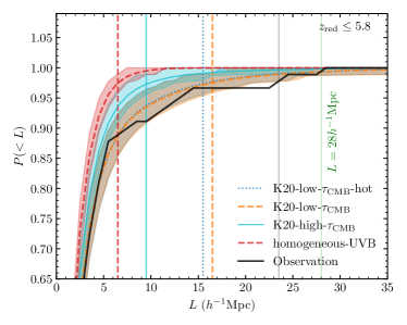
Figure 6: Cumulative distribution of dark gaps that are entirely below $z=5.8$. Vertical colored lines indicate the 97.5 percentile limit for each model. The color shaded regions plot the 68% limit for each model. From left to right are the homogeneous-UVB model, the K20-high-$\tau_{\rm CMB}$ model, and the K20-low-$\tau_{\rm CMB}$-hot model (almost completely overlapped with the K20-low-$\tau_{\rm CMB}$ model), respectively.

Perhaps the most conspicuous feature in the observations is the $L=28{h^{-1}{\rm Mpc}}$ dark gap toward PSO J025$-$11 that extends down to $z\simeq 5.5$. The appearance of this gap may indicate that significant neutral hydrogen islands and/or UVB fluctuations persist down to $z\simeq 5.5$, and provide further leverage for discriminating between models. As the outputs of the ND20 models have no redshift coverage for this dark gap, we only compare the K20 models and the homogeneous-UVB model for this section.

For each model, we use 10,000 bootstrapping realizations to calculate the cumulative distribution function (CDF) of dark gap length, $P(<L)$. Figure 6 compares the observed and predicted $P(<L)$ for dark gaps that are entirely below $z=5.8$. As indicated by the vertical lines, the observed dark gap with $L=28{h^{-1}{\rm Mpc}}$ is well beyond the $95\%$ limits of all the models shown here. These results suggest that the $L=28{h^{-1}{\rm Mpc}}$ gap we observed in the Ly${\beta}$ forest toward PSO J025$-$11 is extremely rare in these models. We perform Mann-Whitey U tests (Mann & Whitney, 1947) for the hypotheses that the distributions of $L$ in the data and predicted by models are equal, for each model respectively. The hypothesis is rejected with $p$-values $<0.05$ for the homogeneous-UVB model.

We further calculate the detection rate of at least one $L=28{h^{-1}{\rm Mpc}}$ gap entirely below $z=5.61$ in the mock samples from each model with the required redshift coverage. We note that in the data there are 10 QSO spectra where the Ly${\beta}$ forest (excluding the proximity zone) covers the full central redshift range of the $L=28{h^{-1}{\rm Mpc}}$ dark gap. We find zero detections of such long dark gaps in the homogeneous-UVB model out of 10,000 trails. The K20-high-$\tau_{\rm CMB}$ model yields a detection rate of $4\%$. Both the K20-low-$\tau_{\rm CMB}$ and K20-low-$\tau_{\rm CMB}$-hot models give higher detection rate of $10\%$. These results suggest that in the case of a late reionization, models with a volume-weighted average neutral hydrogen fraction $\langle x_{\rm HI}\rangle\gtrsim 5\%$ at $z=5.6$ are more consistent with the observations. In addition, the relatively rare presence of $L\geq 28{h^{-1}{\rm Mpc}}$ gaps in the models could also be related to the size of the simulation volume ($160{h^{-1}{\rm Mpc}}$ for the K20 simulations). Simulations run in larger volumes may be needed to compute more accurate statistics on the incidence of these rare, long troughs in late reionization models.

3.3 Neutral Hydrogen Fraction

Figure 7: (a) The mean volume-weighted neutral fraction ($\langle x_{\rm HI}\rangle$) over a Ly${\beta}$ dark gap for a given dark gap length in the mock data. In this figure, “ND20” and “K20” refer to the ND20-late-longmfp model and the K20-low-$\tau_{\rm CMB}$ model, respectively. (b) Distribution of $\langle x_{\rm HI}\rangle$ for a given Ly${\beta}$ dark gap length, $f(x_{\rm HI}|L)$, in the ND20-late-longmfp model at $z=5.6$. $f(x_{\rm HI}|L)$ is normalized for each $L$ interval.

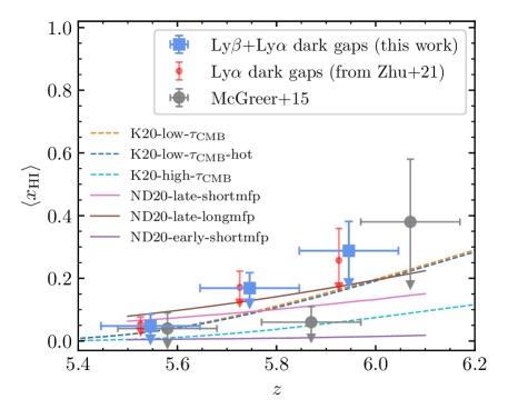
Figure 8: Inference on the neutral hydrogen fraction ($\langle x_{\rm HI}\rangle$) from Ly${\beta}$ dark gaps, which are also dark in the Ly$\alpha$ forest by definition. We show constraints based on Ly$\alpha$ dark gaps from Paper I with red error bars, which are shifted by $-0.02$ in redshift for display. Gray markers plot the constraints based of fraction of pixels that are dark in both the Ly$\alpha$ and Ly${\beta}$ forests from McGreer et al. (2015). The vertical error bars show the $68\%$ ($1\sigma$) limits. The horizontal error bars indicate the $\Delta z=0.2$ redshift bins. For reference, colored lines plot the redshift evolution of $\langle x_{\rm HI}\rangle$ for the reionization models used in this work.

We can further use dark gaps to infer an upper limit on $\langle x_{\rm HI}\rangle$. One can set a strict upper limit on the neutral fraction by assuming that all dark gaps correspond to neutral gas (e.g., McGreer et al., 2011, 2015). At the end of reionization, however, a combination of density and UVB fluctuations will tend to produce dark gaps even once the gas is ionized. We therefore wish to use insights from reionization models to derive a more physically motivated but still conservative upper limit on $\langle x_{\rm HI}\rangle$ from the covering fraction of dark gaps. As described below, we use the fact that dark gaps in the late reionization models tend to show a correlation between the volume-averaged neutral fraction within a gap and the gap length. By applying this relationship to the observed gap length distribution we can set constraints on $\langle x_{\rm HI}\rangle$.

Our goal is to set physically reasonable constraints on $\langle x_{\rm HI}\rangle$ while minimizing the model dependency. We therefore wish to identify the maximum average neutral fraction for a given gap length that is allowed by the models. We first explore the distribution of neutral fractions for a given dark gap length, $f(x_{\rm HI}|L)$. We focus on two models wherein neutral regions contribute significantly to forming dark gaps, the ND20-late-longmfp model and the K20-low-$\tau_{\rm CMB}$ model. Using the mock data, we calculate $x_{\rm HI}$ for each dark gap by averaging the neutral fraction pixel-wise. Figure 7 (a) plots the mean neutral fraction of dark gaps as a function of length, $\langle x_{\rm HI}\rangle_{L}$, at different redshifts. It is related to $f(x_{\rm HI}|L)$ by

$$\langle x_{\rm HI}\rangle_{L}=\int_{0}^{1}x_{\rm HI}f(x_{\rm HI}|L)dx_{\rm HI}.$$ (1)

As shown in the figure, dark gaps of a given length tend to be more neutral as redshift decreases. This is largely because the opacity of the ionized IGM tends to decrease with decreasing redshift, making it more difficult to produce long gaps through density and/or UVB fluctuations alone. In order to set conservative upper limits of $\langle x_{\rm HI}\rangle$ we adopt the $\langle x_{\rm HI}\rangle_{L}$ relationship from ND20-late-longmfp at $z=5.6$. The normalized $f(x_{\rm HI}|L)$ for each dark gap length interval is plotted in Figure 7 (b). This is similar to but slightly higher than the relationship from K20-low-$\tau_{\rm CMB}$ at the same redshift. We also note that the redshift evolution in $\langle x_{\rm HI}\rangle_{L}$ in these models is relatively modest, up to a factor of $\sim$2 in the K20-low-$\tau_{\rm CMB}$ model between $z\sim 6$ and 5.6.

In order to translate the observed gap length distribution into a $\langle x_{\rm HI}\rangle$ constraint, we calculate $\mathscr{F}_{L}$, the fraction of QSO spectra showing dark gaps with length $L$ as a function of redshift. At a certain redshift, the total mean neutral hydrogen fraction is then given by

$$\langle x_{\rm HI}\rangle=\sum_{L=1}^{\infty}\mathscr{F}_{L}\langle x_{\rm HI}\rangle_{L}.$$ (2)

Here we use a sum for $L$ instead of an integral because we measure dark gap lengths in increments of $1{h^{-1}{\rm Mpc}}$. To estimate the uncertainty in $\langle x_{\rm HI}\rangle$, we randomly select the observed sightlines with replacement and calculate the corresponding $\mathscr{F}_{L}$. We use bootstrapping to randomly sample the neutral hydrogen fraction from $f(x_{\rm HI}|L)$ given by models and multiply by the observed $\mathscr{F}_{L}$ of this sample, then sum up for all dark gap lengths. The final uncertainty in $\langle x_{\rm HI}\rangle$ is calculated by repeating this process 10,000 times.

The results are shown in Figure 8. We calculate $\langle x_{\rm HI}\rangle$ in Equation (2) over $\Delta z=0.2$ bins. The inferred upper limits on $\langle x_{\rm HI}\rangle$ are $0.05_{-0.04}^{+0.04}$, $0.17_{-0.05}^{+0.05}$, and $0.29_{-0.10}^{+0.09}$ at $z\simeq 5.55$, 5.75, and 5.95, respectively. We also calculate $\langle x_{\rm HI}\rangle$ following the same method based on Ly$\alpha$ dark gaps presented in Paper I, as shown with red symbols in Figure 8. The Ly$\alpha$ dark gaps yield $\langle x_{\rm HI}\rangle\leq$ $0.05$, $0.17$, and $0.26$ at $z\simeq 5.55$, 5.75, and 5.95, respectively. The measurements based on Ly$\alpha$ and Ly${\beta}$ dark gaps are highly consistent with each other. Compared to the measurements based the fraction of dark pixels by McGreer et al. (2015), our results potentially allow a higher neutral fraction over $5.6\lesssim z\lesssim 6.0$ and a later reionization. The difference in $\langle x_{\rm HI}\rangle$ might be due to cosmic variance and/or the different definitions of dark gaps and dark pixels used in these works. The $\langle x_{\rm HI}\rangle$ measurement at $z\sim 5.9$ in McGreer et al. (2015), moreover, may be biased by transmission peaks in the QSO proximity zone given that their wavelength range for both the Ly$\alpha$ and Ly${\beta}$ forests ends at $z_{\rm QSO}-0.1$, which is less than 6.5 pMpc from the QSO at $z\sim 6$ (see proximity zone size measurements in e.g., Eilers et al., 2017, 2020).

4 Conclusion

In this work, we explore the IGM near the end of reionization using dark gaps in the Ly${\beta}$ forest over $5.5\lesssim z\lesssim 6.0$. We show that about 10%, 40%, and 80% of QSO spectra exhibit long ($L\geq 10{h^{-1}{\rm Mpc}}$) dark gaps in their Ly${\beta}$ forest at $z\simeq 5.6$, 5.8, and 6.0, respectively. Among these gaps, we detect a very long ($L=28{h^{-1}{\rm Mpc}}$) and dark ($\tau_{\rm eff}\gtrsim 6$) Ly${\beta}$ gap extending down to $z\sim 5.5$ toward the $z_{\rm em}=5.85$ QSO PSO J025$-$11.

A comparison between the observed Ly${\beta}$ dark gap statistics for the whole sample of 42 lines of sight and predictions from multiple reionization models (Bolton et al., 2017; Keating et al., 2020a; Nasir & D’Aloisio, 2020) confirms that evidence of reionization in the form of neutral islands and/or a fluctuating UV background persists down to at least $z\sim 5.5$. This supports the conclusions in Paper I and Bosman et al. (2021b). In Paper I we noted a possible tension between Ly$\alpha$ gap statistics and a model wherein reionization ends by $z<6$ but has a relatively early mid-point of $z=8.4$ (Keating et al., 2020a). With Ly${\beta}$ this tension becomes more significant ($>95\%$ level) based on the count of long dark gaps at $z\leq 5.8$, suggesting that very extended reionization scenarios with insufficient remaining neutral hydrogen and/or UVB fluctuations at $z<6$ may be disfavored. In contrast, rapid late reionization models with $\langle x_{\rm HI}\rangle\gtrsim 5\%$ at $z=5.6$ (Keating et al., 2020a; Nasir & D’Aloisio, 2020) are consistent with the observations. A model wherein reionization ends early but retains large-scale fluctuations in the ionizing UV background (Nasir & D’Aloisio, 2020) is also permitted by the dark gap data. We note, however, that recent IGM temperature measurements from Gaikwad et al. (2020) disfavor this model.

A caveat is that we are testing only specific reionization models, including only one with a fluctuating UVB in which reionization ends at $z>6$. By comparison, Gnedin et al. (2017) showed that their full radiative transfer simulations, which reionized near $z\sim 7$, were able to reproduce the Ly$\alpha$ dark gap distribution measured from ESI spectra of a set of twelve $z\sim 6$ QSOs. Because Ly${\beta}$ dark gaps are correlated with Ly$\alpha$ opacities (Appendix A), it is possible that some early reionization scenarios with UVB fluctuations can reproduce our Ly${\beta}$ dark gap distributions while also matching the observed evolution of the mean Ly$\alpha$ transmission.

Finally, we use the observed Ly${\beta}$ gaps to place constraints on the neutral hydrogen fraction based on the association between neutral islands and dark gaps seen in reionization simulations. Our results are broadly consistent with, but more permissive than the constraints from McGreer et al. (2011, 2015) that are based on the dark pixel fraction. Notably, we find an upper limit at $z\simeq 5.75$ of $\langle x_{\rm HI}\rangle\leq 0.17$. This constraint is consistent with scenarios wherein reionization extends significantly below $z=6$.

Appendix A Relationship Between Ly${\beta}$ Dark Gaps and Ly$\alpha$ Dark Gaps

To illustrate the effects of requiring Ly${\beta}$ gaps to also be dark in the Ly$\alpha$ forest, here we explore the relationship between Ly${\beta}$ dark gaps and Ly$\alpha$ dark gaps. In Figure 9 we over-plot Ly${\beta}$-opaque regions ($\rm Flux_{Ly\beta}<0.02$ per $1{h^{-1}{\rm Mpc}}$ bin) on Ly$\alpha$ dark gaps as defined in Paper I. Although Ly${\beta}$-opaque regions overlap strongly with Ly$\alpha$ dark gaps, there do exist regions that are dark only in the Ly${\beta}$ forest, e.g., the long Ly${\beta}$-opaque region toward CFHQS J1509$-$1749 that bridges two Ly$\alpha$ dark gaps, as shown in the figure. These cases are due to foregorund Ly$\alpha$ absorption in the Ly${\beta}$ forest Requiring Ly${\beta}$ gaps to also be dark in the Ly$\alpha$ forest partially avoids this kind of foreground contamination.

We further plot the length of Ly$\alpha$ dark gaps versus the length of corresponding Ly${\beta}$-opaque regions in Figure 10. Most of long ($\geq 10{h^{-1}{\rm Mpc}}$) Ly${\beta}$ dark gaps appear in $L\geq 30{h^{-1}{\rm Mpc}}$ Ly$\alpha$ dark gaps. Only one out of 23 long Ly${\beta}$-opaque regions contains transmission in Ly$\alpha$ and is split into two Ly${\beta}$ dark gaps.

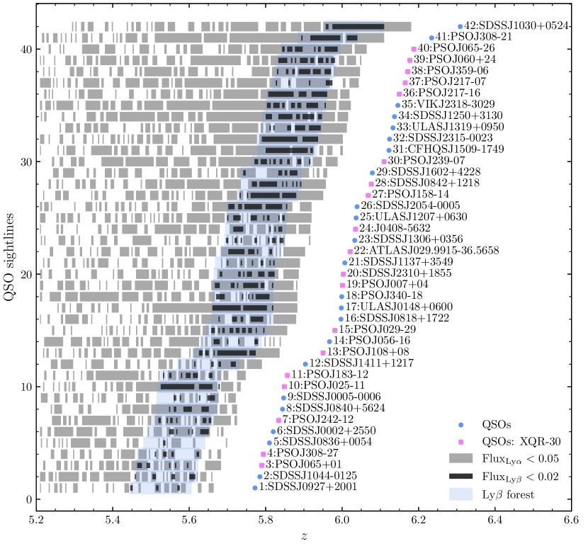
Figure 9: Overview of Ly${\beta}$-opaque regions and Ly$\alpha$ dark gaps from our sample of 42 QSO lines of sight. Black bars show Ly${\beta}$-opaque regions, where normalized flux in the Ly${\beta}$ forest $\rm Flux_{Ly\beta}<0.02$ per $1{h^{-1}{\rm Mpc}}$ bin. Gray bars show Ly$\alpha$ dark gaps as defined in Paper I. Light blue shades highlight the redshift ranges of the Ly${\beta}$ forest. The overlap between the gray bars and black bars yields Ly${\beta}$ dark gaps as defined in this work.

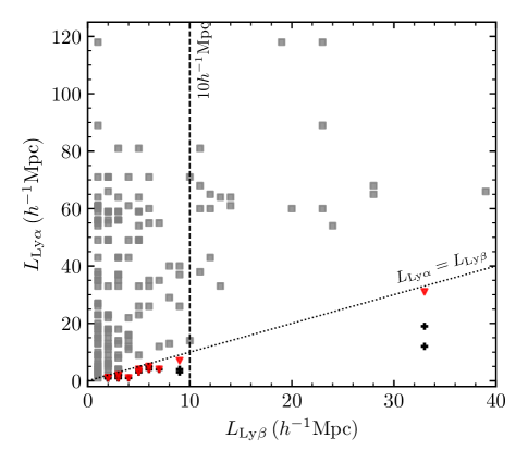
Figure 10: Length of Ly$\alpha$ dark gaps versus length of Ly${\beta}$-opaque regions. For Ly${\beta}$ dark gaps that are entirely within the redshift range of the Ly$\alpha$ dark gap, we plot the length of the Ly$\alpha$ gap versus the length of the Ly${\beta}$ gap with a gray square. Red triangles denote situations where not all $1{h^{-1}{\rm Mpc}}$ pixels in a Ly${\beta}$-opaque region have $\rm Flux_{Ly\alpha}<0.05$ (Ly$\alpha$ dark gaps). The path length of Ly$\alpha$ dark gaps inside these Ly${\beta}$-opaque regions are marked with black crosses.

Appendix B Metal-Enriched Systems

In Figure 11 we display an overview of dark gaps with metal-enriched systems over-plotted for the 27 QSO sightlines in our sample where the identification of metals is relatively complete and consistent. We label metal systems with redshifts in the Ly${\beta}$ forest and in the foreground Ly$\alpha$ forest separately. These systems are included in a metal absorber catalog that will be presented in Davies et al. in prep. Briefly, the Python application Astrocook was used to perform an automated search for Mg II, Fe II, C IV, Si IV, and N V absorbers, and DLA-like systems probed by C II and other low-ionization species. Candidate absorbers were identified using a cross-correlation algorithm within Astrocook that searches for redshifts where significant absorption is present in all relevant transitions. Custom filtering algorithms and visual inspection were then used to remove false positives and produce the final absorber list.

We then investigate the correlation between long ($L\geq 10{h^{-1}{\rm Mpc}}$) dark gaps and metal systems. We find that the probability for a metal system in the Ly${\beta}$ forest to lie in a long dark gap is $15\pm 9\%$, where the $68\%$ confidence limit comes from bootstraping these 27 sightlines 10,000 times. This probability is $31\pm 9\%$ in the case of a system in the corresponding foreground Ly$\alpha$ forest. In these calculations we count clustered metal absorbers with a separation of $<1{h^{-1}{\rm Mpc}}$ as one system. By comparison, the probability that a randomly chosen point lies in a long dark gap is $22\pm 9\%$. Our results suggest that the correlation between long dark gaps and (foreground) metal systems is not highly significant, at least for this sub-sample. The relatively lower probability of finding metal absorbers within the redshifts of long dark gaps nevertheless potentially favors the association between high IGM Ly$\alpha$ opacities and galaxy underdensities (see also Becker et al., 2018; Kashino et al., 2020; Christenson et al., 2021).

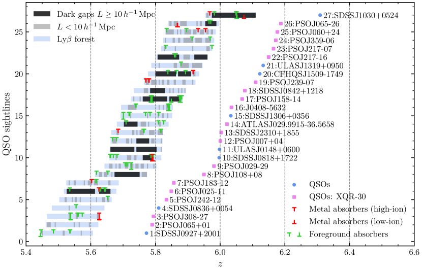
Figure 11: Similar to Figure 2, but with metal-enriched absorbers over-plotted for 27 sightlines that have a relatively complete and consistent identification of metal-enriched absorbers (Davies et al., in prep). We label high-ionization and low-ionization systems within the redshift of the Ly${\beta}$ forest with red “$\top$” and “$\bot$” symbols, respectively. Foreground metal-enriched absorbers whose Ly$\alpha$ absorption would fall within the Ly${\beta}$ forest are labeled with green symbols at the corresponding Ly${\beta}$ redshifts.

Appendix C Uncertainties in the fraction of QSO spectra showing dark gaps

The evolution in $F_{10}$ shown in Figure 4 shows a large drop near $z=5.9$. To estimate the statistical fluctuations in $F_{10}$, we treat the “hit rate” of long dark gaps at individual redshifts as a binomial experiment defined by the number of hits (number of long dark gaps, $n_{\rm dark}$) inside a different number of trials (number of QSO sightlines, $n_{\rm qso}$). At a certain redshift, the posterior probability distribution function for the true “hit rate”, $x$, can be expressed as a Beta distribution, $f(x;\alpha,\beta)\propto x^{\alpha-1}(1-x)^{\beta-1}$, with $\alpha=n_{\rm dark}+0.5$ and $\beta=n_{\rm qso}-n_{\rm dark}+0.5$, assuming a Jeffreys’ prior. As shown in Figure 12 (a), the evolution of $F_{10}$ is consistent with a monotonic increase with $z$ within the 95% confidence intervals. We caution that the analysis here assumes that the “hit rates” at different redshifts are independent from each other.

While the dip could be due to statistical fluctuations, we nevertheless wish to check whether it may relate to possible biases in the data related to Ly${\beta}$ absorption near that redshift. To check for possible systematic effects, we calculate the fraction of QSO spectra showing dark gaps of any length ($L\geq 1{h^{-1}{\rm Mpc}}$) as a function of redshift, $F_{01}$. As shown in Figure 12, the drop in $F_{10}$ at $z\sim 5.9$ is not present in $F_{01}$. Instead, the evolution of Ly${\beta}$-opaque regions with redshift appears relatively smooth. We thus find no evidence of systematic effects in the data that would suggest lower absorption overall near $z=5.9$.

Figure 12: (a) Statistical uncertainty estimation for $F_{10}$ shown in Figure 3 (c). Dark and light shaded regions mark the 68% and 95% limits of $F_{10}$ based on Beta distribution. (b) Fraction of QSO spectra showing dark gaps with $L\geq 1{h^{-1}{\rm Mpc}}$.

Appendix D Dark Gaps in a Lower-redshift Sample

Here we examine the extent to which strong, clustered absorbers associated with galaxies may be able to produce long dark gaps in the Ly${\beta}$ forest. These (typically metal-enriched) absorbers may produce discrete absorption in either Ly${\beta}$ over the redshift over the trough or Ly$\alpha$ at the corresponding foreground redshifts. They may also connect otherwise short dark gaps to form longer gaps. Of particular interest are very long gaps analogous to the $L=28{h^{-1}{\rm Mpc}}$ gap toward PSO J025$-$11. To tests whether such gaps may be due to (circum-)galactic absorbers rather than the IGM, we search for dark gaps at $z\lesssim 5.5$ in a sample of QSO lines of sight that lie at somewhat lower redshifts than our main sample. Because the IGM becomes increasingly transparent toward lower redshifts, any long dark gaps in this sample might signal a significant contribution from discrete systems associated with galaxies.

Our lower-redshift sample includes 27 ESI and X-Shooter spectra of QSOs over $5.0<z_{\rm em}<5.7$ from the Keck and VLT archives. The selection of targets is based on their redshift and is independent from foreknowledge of dark gaps. QSO spectra in this lower-redshift sample have S/N greater than 20 per pixel in the Ly${\beta}$ forest. In order to account for the increased mean transmission at low redshifts, we conservatively use a higher flux threshold of 0.08 when searching for dark gaps. The ratio of mean flux in the Ly${\beta}$ forest at $z=4.8$ and 5.6 is about 3.2 (e.g., Fan et al., 2006; Eilers et al., 2019; Bosman et al., 2021a), thus a flux threshold of 4 times the high-redshift value is used.

Figure 13 shows dark gaps detected in this lower-redshift sample. No dark gaps longer than $10{h^{-1}{\rm Mpc}}$ are detected. The lack of any long gaps in this sample suggests that extended gaps created largely by strong, discrete absorbers are rare, at least over $5\lesssim z\lesssim 5.5$, which is reasonably close in redshift to our main sample. This increases our confidence that the $L=28{h^{-1}{\rm Mpc}}$ dark gap toward PSO J025$-$11 is likely to mainly arise from IGM absorption.

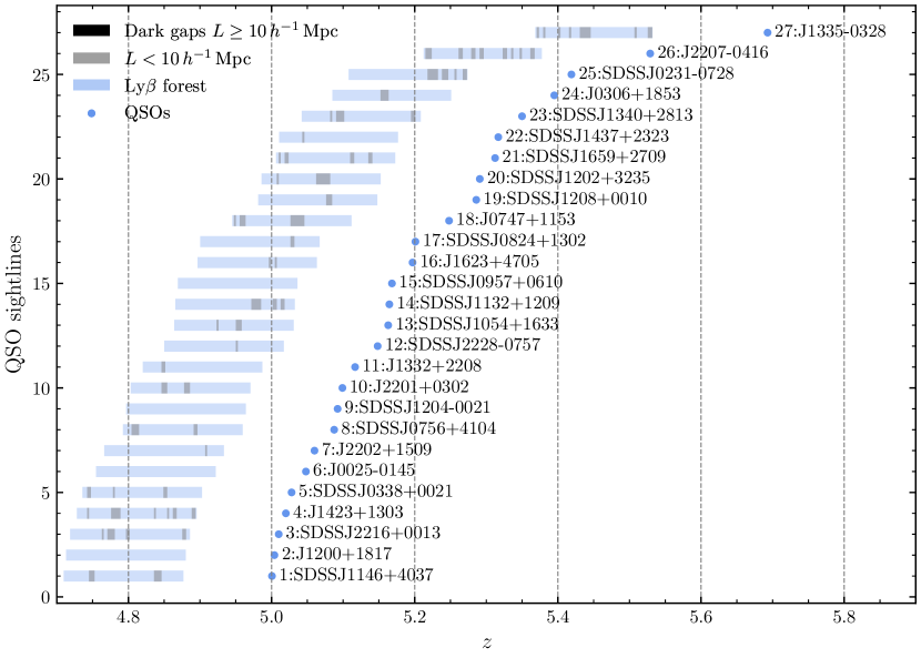
Figure 13: Similar to Figure 2, but showing dark gaps identified in the Ly${\beta}$ forest from a lower-redshift sample.

References

- Astropy Collaboration et al. (2013) Astropy Collaboration, Robitaille, T. P., Tollerud, E. J., et al. 2013, A&A, 558, A33, doi: 10.1051/0004-6361/201322068
- Bañados et al. (2018) Bañados, E., Venemans, B. P., Mazzucchelli, C., et al. 2018, Nature, 553, 473, doi: 10.1038/nature25180
- Becker et al. (2015) Becker, G. D., Bolton, J. S., Madau, P., et al. 2015, MNRAS, 447, 3402, doi: 10.1093/mnras/stu2646
- Becker et al. (2021) Becker, G. D., D’Aloisio, A., Christenson, H. M., et al. 2021, MNRAS, 508, 1853, doi: 10.1093/mnras/stab2696
- Becker et al. (2018) Becker, G. D., Davies, F. B., Furlanetto, S. R., et al. 2018, ApJ, 863, 92, doi: 10.3847/1538-4357/aacc73
- Becker et al. (2019) Becker, G. D., Pettini, M., Rafelski, M., et al. 2019, ApJ, 883, 163, doi: 10.3847/1538-4357/ab3eb5
- Boera et al. (2019) Boera, E., Becker, G. D., Bolton, J. S., & Nasir, F. 2019, ApJ, 872, 101, doi: 10.3847/1538-4357/aafee4
- Bolton et al. (2017) Bolton, J. S., Puchwein, E., Sijacki, D., et al. 2017, MNRAS, 464, 897, doi: 10.1093/mnras/stw2397
- Bosman et al. (2021a) Bosman, S. E. I., Ďurovčíková, D., Davies, F. B., & Eilers, A. C. 2021a, MNRAS, 503, 2077, doi: 10.1093/mnras/stab572
- Bosman et al. (2018) Bosman, S. E. I., Fan, X., Jiang, L., et al. 2018, MNRAS, 479, 1055, doi: 10.1093/mnras/sty1344
- Bosman et al. (2021b) Bosman, S. E. I., Davies, F. B., Becker, G. D., et al. 2021b, arXiv:2108.03699
- Cain et al. (2021) Cain, C., D’Aloisio, A., Gangolli, N., & Becker, G. D. 2021, ApJ, 917, L37, doi: 10.3847/2041-8213/ac1ace
- Carnall (2017) Carnall, A. C. 2017, arXiv:1705.05165
- Choudhury et al. (2021) Choudhury, T. R., Paranjape, A., & Bosman, S. E. I. 2021, MNRAS, 501, 5782, doi: 10.1093/mnras/stab045
- Christenson et al. (2021) Christenson, H. M., Becker, G. D., Furlanetto, S. R., et al. 2021, ApJ, 923, 87, doi: 10.3847/1538-4357/ac2a34
- Cupani et al. (2020) Cupani, G., D’Odorico, V., Cristiani, S., et al. 2020, 11452, 114521U, doi: 10.1117/12.2561343
- Davies et al. (2018a) Davies, F. B., Becker, G. D., & Furlanetto, S. R. 2018a, ApJ, 860, 155, doi: 10.3847/1538-4357/aac2d6
- Davies et al. (2021) Davies, F. B., Bosman, S. E. I., Furlanetto, S. R., Becker, G. D., & D’Aloisio, A. 2021, ApJ, 918, L35, doi: 10.3847/2041-8213/ac1ffb
- Davies et al. (2018b) Davies, F. B., Hennawi, J. F., Bañados, E., et al. 2018b, ApJ, 864, 142, doi: 10.3847/1538-4357/aad6dc
- Davies et al. (2018c) —. 2018c, ApJ, 864, 143, doi: 10.3847/1538-4357/aad7f8
- de Belsunce et al. (2021) de Belsunce, R., Gratton, S., Coulton, W., & Efstathiou, G. 2021, MNRAS, 507, 1072, doi: 10.1093/mnras/stab2215
- Eilers et al. (2018) Eilers, A.-C., Davies, F. B., & Hennawi, J. F. 2018, ApJ, 864, 53, doi: 10.3847/1538-4357/aad4fd
- Eilers et al. (2017) Eilers, A.-C., Davies, F. B., Hennawi, J. F., et al. 2017, ApJ, 840, 24, doi: 10.3847/1538-4357/aa6c60
- Eilers et al. (2019) Eilers, A.-C., Hennawi, J. F., Davies, F. B., & Oñorbe, J. 2019, ApJ, 881, 23, doi: 10.3847/1538-4357/ab2b3f
- Eilers et al. (2020) Eilers, A.-C., Hennawi, J. F., Decarli, R., et al. 2020, ApJ, 900, 37, doi: 10.3847/1538-4357/aba52e
- Fan et al. (2006) Fan, X., Strauss, M. A., Becker, R. H., et al. 2006, AJ, 132, 117, doi: 10.1086/504836
- Furlanetto et al. (2004) Furlanetto, S. R., Hernquist, L., & Zaldarriaga, M. 2004, MNRAS, 354, 695, doi: 10.1111/j.1365-2966.2004.08225.x
- Gaikwad et al. (2021) Gaikwad, P., Srianand, R., Haehnelt, M. G., & Choudhury, T. R. 2021, MNRAS, 506, 4389, doi: 10.1093/mnras/stab2017
- Gaikwad et al. (2020) Gaikwad, P., Rauch, M., Haehnelt, M. G., et al. 2020, MNRAS, 494, 5091, doi: 10.1093/mnras/staa907
- Gallerani et al. (2008) Gallerani, S., Ferrara, A., Fan, X., & Choudhury, T. R. 2008, MNRAS, 386, 359, doi: 10.1111/j.1365-2966.2008.13029.x
- Gnedin et al. (2017) Gnedin, N. Y., Becker, G. D., & Fan, X. 2017, ApJ, 841, 26, doi: 10.3847/1538-4357/aa6c24
- Greig et al. (2021) Greig, B., Mesinger, A., Davies, F. B., et al. 2021, arXiv:2112.04091. https://arxiv.org/abs/2112.04091
- Haardt & Madau (2012) Haardt, F., & Madau, P. 2012, ApJ, 746, 125, doi: 10.1088/0004-637X/746/2/125
- Hoag et al. (2019) Hoag, A., Bradač, M., Huang, K., et al. 2019, ApJ, 878, 12, doi: 10.3847/1538-4357/ab1de7
- Hu et al. (2019) Hu, W., Wang, J., Zheng, Z.-Y., et al. 2019, ApJ, 886, 90, doi: 10.3847/1538-4357/ab4cf4
- Hunter (2007) Hunter, J. D. 2007, CSE, 9, 90, doi: 10.1109/MCSE.2007.55
- Jung et al. (2020) Jung, I., Finkelstein, S. L., Dickinson, M., et al. 2020, ApJ, 904, 144, doi: 10.3847/1538-4357/abbd44
- Kashino et al. (2020) Kashino, D., Lilly, S. J., Shibuya, T., Ouchi, M., & Kashikawa, N. 2020, ApJ, 888, 6, doi: 10.3847/1538-4357/ab5a7d
- Keating et al. (2020a) Keating, L. C., Kulkarni, G., Haehnelt, M. G., Chardin, J., & Aubert, D. 2020a, MNRAS, 497, 906, doi: 10.1093/mnras/staa1909
- Keating et al. (2020b) Keating, L. C., Weinberger, L. H., Kulkarni, G., et al. 2020b, MNRAS, 491, 1736, doi: 10.1093/mnras/stz3083
- Kulkarni et al. (2019) Kulkarni, G., Keating, L. C., Haehnelt, M. G., et al. 2019, MNRAS, 485, L24, doi: 10.1093/mnrasl/slz025
- Mann & Whitney (1947) Mann, H. B., & Whitney, D. R. 1947, The Annals of Mathematical Statistics, 18, 50, doi: 10.1214/aoms/1177730491
- Mason et al. (2018) Mason, C. A., Treu, T., Dijkstra, M., et al. 2018, ApJ, 856, 2, doi: 10.3847/1538-4357/aab0a7
- Mason et al. (2019) Mason, C. A., Fontana, A., Treu, T., et al. 2019, MNRAS, 485, 3947, doi: 10.1093/mnras/stz632
- McGreer et al. (2015) McGreer, I. D., Mesinger, A., & D’Odorico, V. 2015, MNRAS, 447, 499, doi: 10.1093/mnras/stu2449
- McGreer et al. (2011) McGreer, I. D., Mesinger, A., & Fan, X. 2011, MNRAS, 415, 3237, doi: 10.1111/j.1365-2966.2011.18935.x
- Muñoz et al. (2022) Muñoz, J. B., Qin, Y., Mesinger, A., et al. 2022, MNRAS, doi: 10.1093/mnras/stac185
- Nasir & D’Aloisio (2020) Nasir, F., & D’Aloisio, A. 2020, MNRAS, 494, 3080, doi: 10.1093/mnras/staa894
- Paschos & Norman (2005) Paschos, P., & Norman, M. L. 2005, ApJ, 631, 59, doi: 10.1086/431787
- Planck Collaboration et al. (2014) Planck Collaboration, Ade, P. a. R., Aghanim, N., et al. 2014, A&A, 571, A16, doi: 10.1051/0004-6361/201321591
- Planck Collaboration et al. (2020) Planck Collaboration, Aghanim, N., Akrami, Y., et al. 2020, A&A, 641, A6, doi: 10.1051/0004-6361/201833910
- Puchwein et al. (2019) Puchwein, E., Haardt, F., Haehnelt, M. G., & Madau, P. 2019, MNRAS, 485, 47, doi: 10.1093/mnras/stz222
- Qin et al. (2021) Qin, Y., Mesinger, A., Bosman, S. E. I., & Viel, M. 2021, 2101, arXiv:2101.09033. https://arxiv.org/abs/2101.09033
- Sheinis et al. (2002) Sheinis, A. I., Bolte, M., Epps, H. W., et al. 2002, PASP, 114, 851, doi: 10.1086/341706
- Songaila & Cowie (2002) Songaila, A., & Cowie, L. L. 2002, AJ, 123, 2183, doi: 10.1086/340079
- van der Walt et al. (2011) van der Walt, S., Colbert, S. C., & Varoquaux, G. 2011, CSE, 13, 22, doi: 10.1109/MCSE.2011.37
- Vernet et al. (2011) Vernet, J., Dekker, H., D’Odorico, S., et al. 2011, A&A, 536, A105, doi: 10.1051/0004-6361/201117752
- Villasenor et al. (2021) Villasenor, B., Robertson, B., Madau, P., & Schneider, E. 2021, arXiv:2111.00019. https://arxiv.org/abs/2111.00019
- Wang et al. (2020) Wang, F., Davies, F. B., Yang, J., et al. 2020, ApJ, 896, 23, doi: 10.3847/1538-4357/ab8c45
- Weinberger et al. (2019) Weinberger, L. H., Haehnelt, M. G., & Kulkarni, G. 2019, MNRAS, 485, 1350, doi: 10.1093/mnras/stz481
- Wold et al. (2021) Wold, I. G. B., Malhotra, S., Rhoads, J., et al. 2021, arXiv:2105.12191
- Yang et al. (2020a) Yang, J., Wang, F., Fan, X., et al. 2020a, ApJ, 897, L14, doi: 10.3847/2041-8213/ab9c26
- Yang et al. (2020b) —. 2020b, ApJ, 904, 26, doi: 10.3847/1538-4357/abbc1b
- Zhu et al. (2021) Zhu, Y., Becker, G. D., Bosman, S. E. I., et al. 2021, ApJ, 923, 223, doi: 10.3847/1538-4357/ac26c2