Redshifts of radio sources in the Million Quasars Catalogue from machine learning

Abstract

With the aim of using machine learning techniques to obtain photometric redshifts based upon a source’s radio spectrum alone, we have extracted the radio sources from the Million Quasars Catalogue. Of these, 44 119 have a spectroscopic redshift, required for model validation, and for which photometry could be obtained. Using the radio spectral properties as features, we fail to find a model which can reliably predict the redshifts, although there is the suggestion that the models improve with the size of the training sample. Using the near-infrared–optical–ultraviolet bands magnitudes, we obtain reliable predictions based on the 12 503 radio sources which have all of the required photometry. From the 80:20 training–validation split, this gives only 2501 validation sources, although training the sample upon our previous SDSS model gives comparable results for all 12 503 sources. This makes us confident that SkyMapper, which will survey southern sky in the $u,v,g,r,i,z$ bands, can be used to predict the redshifts of radio sources detected with the Square Kilometre Array. By using machine learning to impute the magnitudes missing from much of the sample, we can predict the redshifts for 32 698 sources, an increase from 28% to 74% of the sample, at the cost of increasing the outlier fraction by a factor of 1.4. While the “optical” band data prove successful, at this stage we cannot rule out the possibility of a radio photometric redshift, given sufficient data which may be necessary to overcome the relatively featureless radio spectra.

1 Introduction

There is currently much interest in using machine learning methods to determine the redshifts of distant sources from their photometry. Since forthcoming continuum surveys on the next generation of telescopes are expected yield vast number of new detections, obtaining spectroscopic redshifts for each of these will be too observationally expensive. Of particular interest (to us), is the redshifts of the new sources detected in the radio band with the Square Kilometre Array (SKA), where even just the Australian Square Kilometre Array Pathfinder is expected to yield 70 million radio detections (Norris et al. 2011). Being able to determine the distance to these will greatly increase the scientific value of the surveys. Furthermore, photometric redshifts can be obtained for objects significantly fainter than possible with optical spectroscopy, thus not being as susceptible to bias against the more dust obscured objects, most likely to host cold, star-forming gas, detected through the absorption of the 21-cm transition of hydrogen and the rotational transitions of molecules (Curran et al., 2011; Curran & Whiting, 2012; Curran, 2021).

Finding a photometric redshift based upon the radio spectrum alone has so far proven elusive (Majic & Curran, 2015; Norris et al., 2019), most likely due to the relatively featureless spectra, whereas machine learning techniques using the near-infrared–optical–ultra-violet photometry have proven successful (Bovy et al., 2012; Brescia et al., 2013; Carvajal et al., 2021; Nakoneczny et al., 2021). These are usually trained and validated upon the same sample, typically from the Sloan Digital Sky Survey (SDSS), although Curran (2020); Curran et al. (2021) have demonstrated that an SDSS trained model can reliably predict the redshifts of quasars from external catalogues of radio-selected sources.

Turner et al. (2020) have used the radio fluxes at 151, 178 and 2700 MHz, combined with imaging of the radio lobes, to predict the redshifts of nine sources, although it is not clear how this will scale to large samples where the emission may be spatially unresolved. Ideally, we wish to be able to predict the redshifts from the radio spectral energy distribution (SED) alone, although as discussed by Curran & Moss (2019), there is a dearth of large radio catalogues for which we also have accurate spectroscopic redshifts (Morganti et al., 2015), required to enable validation of the predictions.

In this paper, we therefore extract the radio sources in the 1 573 822 strong Million Quasars Catalogue (Milliquas, Flesch 2021) and explore the potential of this sample in the prediction of radio photometric redshifts. We also test the accuracy of a model constructed from the near-infrared–optical–ultra-violet of the Milliquas in predicting redshifts for radio-selected sources.

2 The data

2.1 The sample

The Milliquas comprises 1 573 822 quasi-stellar objects (QSOs) compiled from the literature, including SDSS QSOs up to Data Release 16 (Flesch 2015, 2021). Of these, there are 136 076 with a radio association, of which 44 495 have a spectroscopic redshift.

2.2 Photometry extraction

Similarly to what we did in Curran et al. (2021), each of the final 44 495 sources was matched to a source in the NASA/IPAC Extragalactic Database (NED). Matches were found for 44 119, for which we scraped all of the photometry, including the radio-band data. Since the $W2,W1,z,i,r,g,u,NUV,FUV$ photometry have a proven track record in the use of machine learning to predict redshifts (Sect. 1), we used the NED names to query the Wide-Field Infrared Survey Explorer (WISE), the Two Micron All Sky Survey (2MASS, Skrutskie et al. 2006) databases for the near-infrared (NIR) and the GALEX database (Bianchi et al., 2017) for ultra-violet (UV) photometry.

2.3 Photometry fitting

2.3.1 Radio fitting and features

The combination of NIR, optical and UV colours have been very successful when used as features for machine learning models and artificial neural networks, with the raw magnitudes appearing to perform as well as the colour indices (Curran et al., 2021; Curran, 2022). We therefore use the analogous radio features here, specifically the flux density at various frequencies. As per the NIR–optical–UV fitting (see Sect. 2.3.2), we select several commonly observed bands and average the fluxes within each of these for each source, specifically at 70 MHz (over 70–80 MHz), 150 MHz (150–160 MHz), 400 MHz (365–408 MHz), 700 MHz (635–750 MHz), 1 GHz (960–1100 MHz), 1.4 GHz (1.3–1.5 GHz), 2.7 GHz (2.6–2.7 GHz), 5 GHz (4.7–5.0 GHz), 8.7 GHz (7.9–8.9 GHz), 15 GHz (14–16 GHz) and 20 GHz (20–24 GHz).

In order to test for a turnover in the SED, we also fit a second order polynomial to the radio photometry (see Curran et al. 2013). This was used to determine the spectral index at 1.4 GHz, $\alpha_{1.4~{}\text{GHz}}$, as well as providing the initial parameters to fit a function of the form (Snellen et al., 1998)

$$S=\frac{S_{\text{peak}}}{1-1/e}\left(\frac{\nu}{\nu_{\text{peak}}}\right)^{\alpha_{\text{thick}}}\left(1-\exp\left\{-\left(\frac{\nu}{\nu_{\text{peak}}}\right)^{\alpha_{\text{thin}}-\alpha_{\text{thick}}}\right\}\right),$$

where $S_{\text{peak}}$ is the flux density at the turnover frequency, $\nu_{\text{peak}}$, $\alpha_{\text{thick}}$ the spectral index of optically thick part of spectrum and $\alpha_{\text{thin}}$ the spectral index of optically thin part of spectrum (Fig. 1).

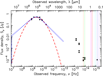
Figure 1: Example of the radio-band fitting to the photometry. The red broken curve shows the second order polynomial fitting, giving $\nu_{\text{TO}}$, the blue dotted curve the Snellen et al. fit, giving $\nu_{\text{peak}}$, $\alpha_{\text{thin}}$ (to the left of $\nu_{\text{peak}}$) and $\alpha_{\text{thick}}$ (to the right of $\nu_{\text{peak}}$). The dotted vertical lines show the location of the $W2,W1,z,i,r,g,u,NUV,FUV$ bands.

We summarise these potential features in Table 1,

Table 1: Potential features in the classification of the radio spectra (see Fig. 2).

Feature(s)	Description
$\log_{10}S_{\text{70 MHz}}$ to $\log_{10}S_{\text{20 GHz}}$	Log flux densities at 70, 150, 400 & 700  MHz and 1.0, 1.4, 2.7, 5.0. 8.7, 15 & 20 GHz
Polynomial fit
$\alpha_{1.4~{}\text{GHz}}$	Spectral index at 1.4 GHz
$X_{2},X_{1},X_{0}$	Coefficients of the polynomial fit, $\log_{10}S=X_{2}\log_{10}\nu^{2}+X_{1}\log_{10}\nu+\log_{10}X_{0}$
$\log_{10}\nu_{\text{TO}}$	Log turnover frequency of the fit, i.e. where $dS/d\nu=-X_{1}/2X_{2}=0$
$\log_{10}S_{\text{TO}}$	Log flux density at turnover frequency
Additional parameters from Snellen et al. fit
$\log_{10}\nu_{\text{peak}}$	Log turnover frequency of the fit
$\log_{10}S_{\text{peak}}$	Log flux density at turnover frequency
$\alpha_{\text{thin}}$	Spectral index of optically thin part of spectrum
$\alpha_{\text{thick}}$	Spectral index of optically thick part of spectrum

and show their redshift distributions in Fig. 2.

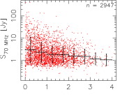
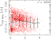
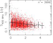
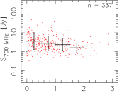
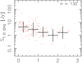
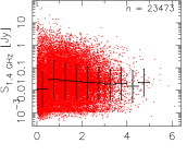
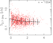
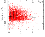
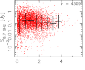
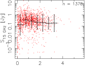
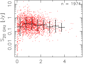
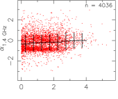
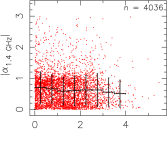
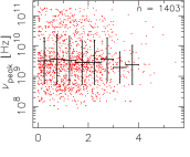
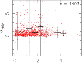
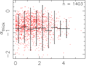
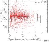
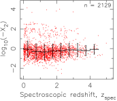
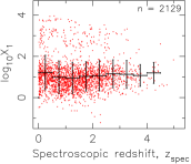
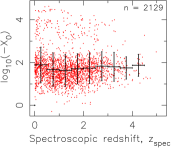
Figure 2: Distributions of potential radio features with redshift. The binning is for equal redshift spacing, with the error bars on the ordinate showing the mean value $\pm 1\sigma$.

From these (Table 2), we

Table 2: The feature redshift correlations (Fig. 2). The number of sources is followed by the Kendall-tau test probability of the observed correlation arising by chance and the significance of the correlation ($Z$-value), assuming Gaussian statistics.

Feature	$n$	$P(\tau)$	$Z(\tau)$
$\log_{10}S_{\text{70 MHz}}$	2947	$1.15\times 10^{-26}$	$10.60\sigma$
$\log_{10}S_{\text{150 MHz}}$	3059	0.319	$0.97\sigma$
$\log_{10}S_{\text{400 MHz}}$	3999	$2.27\times 10^{-31}$	$11.65\sigma$
$\log_{10}S_{\text{700 MHz}}$	337	$1.51\times 10^{-8}$	$5.66\sigma$
$\log_{10}S_{\text{1.0 GHz}}$	132	$6.25\times 10^{-6}$	$4.25\sigma$
$\log_{10}S_{\text{1.4 GHz}}$	23 473	$7.16\times 10^{-141}$	$19.70\sigma$
$\log_{10}S_{\text{2.7 GHz}}$	1554	$1.29\times 10^{-11}$	$6.77\sigma$
$\log_{10}S_{\text{5.0 GHz}}$	7239	0.379	$0.88\sigma$
$\log_{10}S_{\text{8.7 GHz}}$	4309	0.963	$0.05\sigma$
$\log_{10}S_{\text{15 GHz}}$	1378	0.721	$0.36\sigma$
$\log_{10}S_{\text{20 GHz}}$	1974	0.269	$1.11\sigma$
$\alpha_{1.4~{}\text{GHz}}$	4036	$4.45\times 10^{-15}$	$7.84\sigma$
$|\alpha_{1.4~{}\text{GHz}}|$	4036	$6.36\times 10^{-9}$	$5.81\sigma$
$\log_{10}\nu_{\text{peak}}$	1403	0.342	$0.95\sigma$
$\log_{10}S_{\text{peak}}$	1403	0.017	$2.40\sigma$
$\alpha_{\text{thin}}$	1403	0.190	$1.31\sigma$
$\alpha_{\text{thick}}$	1403	0.960	$0.05\sigma$
$\log_{10}\nu_{\text{TO}}$	2129	0.125	$1.59\sigma$
$\log_{10}S_{\text{TO}}$	2129	0.230	$1.20\sigma$
$\log_{10}(-X_{2})$	2129	0.754	$0.31\sigma$
$\log_{10}X_{1}$	2129	0.772	$0.29\sigma$
$\log_{10}(-X_{0})$	2129	0.785	$0.27\sigma$

see that, as expected, the flux densities are generally anti-correlated with the redshift. Apart from these, the only other parameter strongly correlated with the redshift is the spectral index, $\alpha_{1.4~{}\text{GHz}}$. A positive correlation between spectral index and radio luminosity (and therefore redshift) has been previously noted for 69 radio galaxies and quasars by Bridle et al. (1972), with Athreya & Kapahi (1998) finding a positive correlation for 15 $z>2$ radio galaxies. Also, like O’Dea & Baum (1997), we find no correlation with the turnover frequency (cf. Menon 1983). Finally, in Table LABEL:intersect_all, we list the number of features common to the sources,

Table 3: Features common to the sources in (column) descending order of sample size (Table 2). $n_{\text{int}}$ gives the accumulated intersection of features, $\log_{10}S_{\text{1.4 GHz}}\cap\log_{10}S_{\text{5.0 GHz}}$ in the second row, followed in $\log_{10}S_{\text{1.4 GHz}}\cap\log_{10}S_{\text{5.0 GHz}}\cap\alpha_{1.4~{}\text{GHz}}$ in the third row, etc.

Feature	$n$	$n_{\text{int}}$	Feature	$n$	$n_{\text{int}}$
Whole sample
$\log_{10}S_{\text{1.4 GHz}}$	23 473	23 473	Polynomial fit	2129	76
$\log_{10}S_{\text{5.0 GHz}}$	7239	6808	$\log_{10}S_{\text{20 GHz}}$	1974	60
$\log_{10}S_{\text{8.7 GHz}}$	4309	3691	$\log_{10}S_{\text{2.7 GHz}}$	1554	45
$\alpha_{1.4~{}\text{GHz}}$	4036	2058	Snellen et al. fit	1403	42
$\log_{10}S_{\text{400 MHz}}$	3999	1001	$\log_{10}S_{\text{15 GHz}}$	1378	39
$\log_{10}S_{\text{150 MHz}}$	3059	351	$\log_{10}S_{\text{700 MHz}}$	337	25
$\log_{10}S_{\text{70 MHz}}$	2947	253	$\log_{10}S_{\text{1.0 GHz}}$	132	12
Most populous with polynomial fit (poly sample)
Polynomial fit	2129	2129	$\log_{10}S_{\text{8.7 GHz}}$	4309	1421
$\log_{10}S_{\text{1.4 GHz}}$	23 473	1976	$\alpha_{1.4~{}\text{GHz}}$	4036	1416
$\log_{10}S_{\text{5.0 GHz}}$	7239	1744	$\log_{10}S_{\text{400 MHz}}$	3999	559
Most populous with Snellen et al. fit (snellen sample)
Snellen et al. fit	1403	1403	$\log_{10}S_{\text{8.7 GHz}}$	4309	991
$\log_{10}S_{\text{1.4 GHz}}$	23 473	1289	$\alpha_{1.4~{}\text{GHz}}$	4036	990
$\log_{10}S_{\text{5.0 GHz}}$	7239	1163	$\log_{10}S_{\text{400 MHz}}$	3999	478
Flux densities only (flux sample)
$\log_{10}S_{\text{1.4 GHz}}$	23 473	23 473	$\log_{10}S_{\text{20 GHz}}$	1974	329
$\log_{10}S_{\text{5.0 GHz}}$	7239	6808	$\log_{10}S_{\text{2.7 GHz}}$	1554	233
$\log_{10}S_{\text{8.7 GHz}}$	4309	3691	$\log_{10}S_{\text{15 GHz}}$	1378	137
$\log_{10}S_{\text{400 MHz}}$	3999	2037	$\log_{10}S_{\text{700 MHz}}$	337	83
$\log_{10}S_{\text{150 MHz}}$	3059	716	$\log_{10}S_{\text{1.0 GHz}}$	132	48
$\log_{10}S_{\text{70 MHz}}$	2947	549

from which we see only 12 of the 44 119 have all features.

2.3.2 NIR–optical–UV fitting

As before (Curran et al., 2021), for the optical-band photometry the PSF flux densities associated with the AB magnitudes of the Sloan Digital Sky Survey (SDSS) were used. We chose these as they are the most extensive available and are the standard choice in using machine learning to obtain photometric redshifts (e.g. Richards et al. 2001; Weinstein et al. 2004; Maddox et al. 2012; Han et al. 2016). In order to be applicable to samples for which the SDSS, WISE and GALEX photometry may not be directly available, including the current sample, we collected data which fall within $\Delta\log_{10}\nu=\pm 0.05$ of the central frequency of each of the bands. Within each band the fluxes were then averaged before being converted to a magnitude. Of the 44 119 radio sources, there were 12 503 which had all nine of the required magnitudes.

3 Methodology

3.1 Machine Learning

We tested three machine learning algorithms, in addition to an Artificial Neural Network (ANN) algorithm. For the machine learning we used $k$-Nearest Neighbour Regressor (kNN), Support Vector Regression (SVR) and Decision Tree Regression (DTR), which were initally tested with the default hyperparameters (see https://scikit-learn.org/stable/). After experimenting with these, we settled on:

• kNN – uniform weighting and $k\approx 10-25$ nearest neighbours,

• SVR – $C\approx 50$, $\gamma=0.1$ and $\epsilon=0.1$ (cf. the default parameters $C=10$, $\gamma=$ scale and $\epsilon=0.1$),

• DTR – maximum depth of 4 – 12,

depending on the dataset (Sect. 4.1). Note that, perhaps due to the small sample sizes, the algorithms were fairly insensitive to the hyperparameters (especially over many trials, see Table 4). Also, when close to what appeared to be the optimum model, tweaking the models could move the metrics in opposite directions, e.g. an increase in the regression coefficient together with an increase in the spread between the predicted and measured redshifts (see below).

Although samples which included a relatively large number of features were few (Sect. 2.3.1), we also tested an ANN algorithm, primarily to gauge just how small the sample could be before this failed to compete with the machine learning models. Artificial neutral networks use a computer architecture based upon neurons in a brain, where the artificial neuron is the functional unit of the network which comprises several layers – an input layer, weighting and biasing of the features, and several layers containing non-linear activation functions, which transform the weighted input features. Each neuron may be connected from one to all of the others in adjacent layers. We used the TensorFlow platform, with the testing of various hyperparameters giving the best results using a model similar to that in Curran et al. (2021), that is two ReLu layers and one tanh layer comprising $\stackrel{{\scriptstyle>}}{{{}_{\sim}}}50$ to $\stackrel{{\scriptstyle<}}{{{}_{\sim}}}200$ neurons each (Fig. 3).

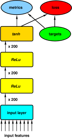
Figure 3: Architecture of the neural network used in the artificial neutral network.

That is:

1. An input layer with one neuron for each training feature, e.g. $\log_{10}\nu_{\text{TO}}$, $\log_{10}S_{\text{TO}}$, $\log_{10}(-X_{2})$, $\log_{10}X_{1}$, $\log_{10}(-X_{0})$, $\log_{10}S_{\text{1.4 GHz}}$, $\log_{10}S_{\text{5.0 GHz}}$, $\log_{10}S_{\text{8.7 GHz}}$ and $\alpha_{1.4~{}\text{GHz}}$, for the $n_{\text{int}}\geq 1416$, poly sample.

2. Three dense layers, each with 200 neurons, the first two using $ReLu$ activation functions and the third a $tanh$ function.,

3. One output layer for the target (the photometric redshift for the source).

3.2 Metrics

For each of the algorithms, we normalised the features and used a 80:20 training–validation split. We quantified the quality of the redshift prediction according to:

1. The regression coefficient, $r$, of the least-squares linear fit between the predicted $(z_{\rm phot}$) and measured ($z_{\rm spec}$) redshifts.

2. The standard deviation from the mean difference between the photometric and spectroscopic redshifts, $\Delta z\equiv z_{\rm spec}-z_{\rm phot}$,

   $$\sigma_{\Delta z}\equiv\sqrt{\frac{1}{N}\sum_{i=1}^{N}\Delta z^{2}},$$

   in addition to the normalised standard deviation, obtained from $\Delta z(\text{norm})=\Delta z/({z_{\rm spec}+1})$.

3. The median absolute deviation (MAD),

   $$\sigma_{\text{MAD}}\equiv 1.48\times\text{median}\left|\Delta z\right|,$$

   in addition to the normalised median absolute deviation (NMAD),

   $$\sigma_{\text{NMAD}}\equiv 1.48\times\text{median}\left|\Delta z(\text{norm})\right|.$$

4. The outlier fraction (e.g. Carvajal et al. 2021; Li et al. 2021),

   $$\eta\equiv\frac{n_{|\Delta z(\text{norm})|>0.15}}{n},$$

   that is, the number of sources with $|\Delta z(\text{norm})|>0.15$ as a fraction of the total number.

4 Results

4.1 Radio photometric redshifts

As discussed in Sect. 2.3.1, the number of sources available decreases rapidly as more radio-band features are added. Therefore, we test three different samples, ranging from the most features/least sources to least features/most sources:

1. Peaked spectrum sources only, where the turnover parameters are included as features. This is split into two sub-samples:

   1. The poly sample: Those for which a polynomial is fit, thus including $\log_{10}\nu_{\text{TO}}$ , $\log_{10}S_{\text{TO}}$, $\log_{10}(-X_{2})$, $\log_{10}X_{1}$ and $\log_{10}(-X_{0})$ as features.

   2. The snellen sample: The subset of these which could be fit by the function of Snellen et al. (1998), thus including $\log_{10}\nu_{\text{peak}}$, $\log_{10}S_{\text{peak}}$, $\alpha_{\text{thin}}$ and $\alpha_{\text{thick}}$ as features.

2. The ohe sample: All of the sources, where the presence of a turnover in the SED was one-hot encoded as a feature. Thus, in addition to the flux densities at different frequencies, the model contained two distinct sub-samples:

   1. Sources which exhibited a peak in the radio SED.

   2. Sources where the SED exhibits no peak, which may be

      1. flat spectrum, with $|\alpha_{1.4~{}\text{GHz}}|\stackrel{{\scriptstyle<}}{{{}_{\sim}}}0.5$,

      2. steep spectrum, with $\alpha_{1.4~{}\text{GHz}}\stackrel{{\scriptstyle<}}{{{}_{\sim}}}-0.5$, or

      3. inverted spectrum, with $\alpha_{1.4~{}\text{GHz}}\stackrel{{\scriptstyle>}}{{{}_{\sim}}}0.5$,

      and where $\alpha_{1.4~{}\text{GHz}}$ may be correlated with the redshift (Sect. 2.3.1).

3. The flux sample: All of the sources, using only the flux densities at different frequencies as features. This is most analogous to the optical-band techniques, which utilise the source magnitudes.

Since the 80:20 training–validation split applied to such small sample sizes can lead to “(un)lucky” results, we ran each algorithm 100 times, randomising the training and validation sources for each trial.

4.1.1 Peaked spectrum sources

1403 of the sources with sufficient radio photometry exhibited a turnover which could be fit by the function of Snellen et al. (1998) and 2129 by a second order polynomial (Sect. 2.3.1). However, referring to Table LABEL:intersect_all, we see that the inclusion of other features significantly decreases the sample size. We therefore used the features for which $n_{\text{int}}\geq 1416$, prioritised by the fit, starting with the polynomial (Table LABEL:intersect_all).

When training and validating upon the NIR–optical–UV magnitudes (Curran et al. 2021 and references therein) we achieve $r\stackrel{{\scriptstyle>}}{{{}_{\sim}}}0.9$, $\sigma_{\Delta z(\text{norm})}\stackrel{{\scriptstyle<}}{{{}_{\sim}}}0.3$ and $\sigma_{\text{NMAD}}\stackrel{{\scriptstyle<}}{{{}_{\sim}}}0.1$. Using this as a benchmark, from Table 4 we see that all algorithms perform poorly with little predictive power.

Table 4: The mean values $\pm 1\sigma$ of 100 trials of the machine learning algorithms, where the training and validation sets are randomised for each trial. In addition to the metrics listed in Sect. 3.2, we quote the mean bias in $\Delta z$, $\mu_{\Delta z}$, and normalised bias, $\mu_{\Delta z(\text{norm})}$.

Regressor		Un-normalised			Normalised
	$r$	$\mu_{\Delta z}$	$\sigma_{\Delta z}$	$\sigma_{\text{MAD}}$	$\mu_{\Delta z(\text{norm})}$	$\sigma_{\Delta z(\text{norm})}$	$\sigma_{\text{NMAD}}$	$\eta$
$n_{\text{int}}\geq 1416$ of the poly sample (284 validation sources)
kNN	$0.16\pm 0.05$	$-0.02\pm 0.06$	$0.92\pm 0.04$	$0.92\pm 0.06$	$-0.16\pm 0.03$	$0.48\pm 0.03$	$0.37\pm 0.02$	$67.6\pm 2.5$%
SVR	$0.20\pm 0.05$	$0.07\pm 0.05$	$0.90\pm 0.04$	$0.93\pm 0.06$	$-0.11\pm 0.03$	$0.45\pm 0.02$	$0.36\pm 0.02$	$68.6\pm 2.2$%
DTR	$0.13\pm 0.05$	$-0.01\pm 0.06$	$0.92\pm 0.04$	$0.96\pm 0.06$	$-0.15\pm 0.03$	$0.47\pm 0.02$	$0.38\pm 0.02$	$68.5\pm 2.4$%
ANN	$0.17\pm 0.04$	$0.00\pm 0.28$	$0.96\pm 0.02$	$0.89\pm 0.06$	$-0.14\pm 0.08$	$0.46\pm 0.03$	$0.36\pm 0.07$	$67.8\pm 2.3$%
$n_{\text{int}}\geq 990$ of the snellen sample (198 validation sources)
kNN	$0.14\pm 0.07$	$-0.02\pm 0.06$	$0.93\pm 0.05$	$0.95\pm 0.07$	$-0.16\pm 0.03$	$0.48\pm 0.03$	$0.38\pm 0.03$	$70.0\pm 2.8$%
SVR	$0.14\pm 0.06$	$0.06\pm 0.07$	$0.92\pm 0.05$	$0.94\pm 0.07$	$-0.12\pm 0.03$	$0.46\pm 0.03$	$0.38\pm 0.03$	$71.3\pm 2.7$%
DTR	$0.06\pm 0.06$	$0.01\pm 0.08$	$0.94\pm 0.04$	$0.99\pm 0.07$	$-0.15\pm 0.04$	$0.48\pm 0.03$	$0.39\pm 0.03$	$69.7\pm 3.0$%
ANN	$0.13\pm 0.04$	$0.17\pm 0.16$	$0.97\pm 0.02$	$0.94\pm 0.05$	$-0.07\pm 0.07$	$0.46\pm 0.03$	$0.38\pm 0.02$	$70.7\pm 2.8$%
$n_{\text{int}}\geq 1001$ of the ohe sample (201 validation sources)
kNN	$0.34\pm 0.06$	$-0.04\pm 0.07$	$0.83\pm 0.04$	$0.83\pm 0.06$	$-0.15\pm 0.04$	$0.44\pm 0.03$	$0.36\pm 0.03$	$67.7\pm 3.0$%
SVR	$0.35\pm 0.05$	$0.05\pm 0.07$	$0.82\pm 0.04$	$0.79\pm 0.07$	$-0.11\pm 0.04$	$0.43\pm 0.03$	$0.34\pm 0.03$	$65.7\pm 3.1$%
DTR	$0.30\pm 0.06$	$-0.00\pm 0.07$	$0.85\pm 0.04$	$0.87\pm 0.07$	$-0.14\pm 0.04$	$0.44\pm 0.03$	$0.37\pm 0.04$	$68.2\pm 3.1$%
ANN	$0.30\pm 0.03$	$-0.08\pm 0.12$	$0.93\pm 0.01$	$0.91\pm 0.05$	$-0.20\pm 0.06$	$0.49\pm 0.03$	$0.40\pm 0.03$	$70.5\pm 2.6$%
$n_{\text{int}}\geq 351$ of the ohe sample (71 validation sources)
kNN	$0.41\pm 0.09$	$-0.01\pm 0.10$	$0.77\pm 0.08$	$0.72\pm 0.09$	$-0.13\pm 0.05$	$0.40\pm 0.05$	$0.38\pm 0.05$	$70.5\pm 5.0$%
SVR	$0.46\pm 0.09$	$0.09\pm 0.10$	$0.77\pm 0.08$	$0.70\pm 0.09$	$-0.06\pm 0.05$	$0.40\pm 0.05$	$0.34\pm 0.05$	$65.5\pm 5.2$%
DTR	$0.31\pm 0.11$	$0.01\pm 0.12$	$0.84\pm 0.08$	$0.75\pm 0.09$	$-0.12\pm 0.06$	$0.43\pm 0.06$	$0.37\pm 0.04$	$70.0\pm 5.0$%
ANN	$0.39\pm 0.03$	$-0.13\pm 0.16$	$0.80\pm 0.02$	$0.79\pm 0.08$	$-0.19\pm 0.08$	$0.43\pm 0.03$	$0.36\pm 0.05$	$67.2\pm 4.4$%
$n_{\text{int}}\geq 2037$ of the flux sample (408 validation sources)
kNN	$0.29\pm 0.49$	$-0.03\pm 0.04$	$0.78\pm 0.03$	$0.80\pm 0.04$	$-0.14\pm 0.02$	$0.41\pm 0.01$	$0.37\pm 0.02$	$68.6\pm 1.8$%
SVR	$0.30\pm 0.04$	$0.10\pm 0.04$	$0.78\pm 0.03$	$0.76\pm 0.04$	$-0.08\pm 0.02$	$0.39\pm 0.02$	$0.36\pm 0.02$	$68.1\pm 2.1$%
DTR	$0.23\pm 0.04$	$0.00\pm 0.04$	$0.80\pm 0.03$	$0.81\pm 0.04$	$-0.13\pm 0.02$	$0.43\pm 0.02$	$0.37\pm 0.02$	$69.1\pm 2.0$%
ANN	$0.28\pm 0.04$	$0.00\pm 0.10$	$0.78\pm 0.03$	$0.80\pm 0.05$	$-0.13\pm\pm 0.05$	$0.42\pm 0.02$	$0.36\pm 0.02$	$67.9\pm 2.4$%
$n_{\text{int}}\geq 716$ of the flux sample (144 validation sources)
kNN	$0.36\pm 0.06$	$-0.03\pm 0.07$	$0.73\pm 0.05$	$0.73\pm 0.06$	$-0.13\pm 0.04$	$0.39\pm 0.02$	$0.38\pm 0.03$	$69.4\pm 3.6$%
SVR	$0.38\pm 0.06$	$0.09\pm 0.06$	$0.72\pm 0.04$	$0.65\pm 0.05$	$-0.06\pm 0.03$	$0.36\pm 0.02$	$0.34\pm 0.03$	$65.9\pm 3.9$%
DTR	$0.31\pm 0.07$	$0.01\pm 0.07$	$9.76\pm 0.06$	$0.73\pm 0.07$	$-0.11\pm 0.04$	$0.40\pm 0.03$	$0.37\pm 0.03$	$67.4\pm 4.0$%
ANN	$0.33\pm 0.08$	$0.02\pm 0.20$	$0.75\pm 0.05$	$0.73\pm 0.09$	$-0.10\pm 0.10$	$0.40\pm 0.04$	$0.37\pm 0.04$	$69.9\pm 4.4$%
$n_{\text{int}}\geq 549$ of the flux sample (110 validation sources)
kNN	$0.36\pm 0.08$	$-0.03\pm 0.08$	$0.66\pm 0.04$	$0.67\pm 0.06$	$-0.12\pm 0.05$	$0.35\pm 0.03$	$0.36\pm 0.03$	$68.2\pm 4.0$%
SVR	$0.37\pm 0.06$	$0.09\pm 0.07$	$0.66\pm 0.07$	$0.60\pm 0.06$	$-0.05\pm 0.04$	$0.33\pm 0.02$	$0.33\pm 0.33$	$63.6\pm 4.3$%
DTR	$0.30\pm 0.08$	$0.00\pm 0.08$	$0.70\pm 0.04$	$0.68\pm 0.07$	$-0.10\pm 0.04$	$0.37\pm 0.03$	$0.36\pm 0.04$	$67.3\pm 4.4$%
ANN	$0.30\pm 0.09$	$0.01\pm 0.14$	$0.70\pm 0.05$	$0.70\pm 0.10$	$-0.10\pm 0.08$	$0.38\pm 0.04$	$0.37\pm 0.05$	$68.2\pm 5.1$%
$n_{\text{int}}\geq 329$ of the flux sample (66 validation sources)
kNN	$0.26\pm 0.11$	$-0.05\pm 0.09$	$0.63\pm 0.06$	$0.67\pm 0.08$	$-0.13\pm 0.05$	$0.34\pm 0.03$	$0.37\pm 0.04$	$67.8\pm 5.6$%
SVR	$0.27\pm 0.09$	$0.09\pm 0.10$	$0.64\pm 0.06$	$0.58\pm 0.08$	$-0.05\pm 0.05$	$0.32\pm 0.03$	$0.31\pm 0.05$	$62.6\pm 5.3$%
DTR	$0.27\pm 0.11$	$0.00\pm 0.09$	$0.65\pm 0.06$	$0.65\pm 0.09$	$-0.10\pm 0.05$	$0.35\pm 0.03$	$0.35\pm 0.04$	$64.8\pm 5.2$%
ANN	$0.19\pm 0.12$	$-0.001\pm 0.17$	$0.69\pm 0.06$	$0.72\pm 0.10$	$-0.10\pm 0.09$	$0.39\pm 0.04$	$0.39\pm 0.05$	$69.4\pm 5.5$%

Adding the next populous feature, $\log_{10}S_{\text{400 MHz}}$, giving $n_{\text{int}}\geq 559$ and a validation sample size of 112, gave no improvement in the predictions. Repeating the procedure for the SED fit of Snellen et al., gives the sample sizes listed in Table LABEL:intersect_all and again, poor results (Table 4).

4.1.2 All radio sources

Testing all of the radio sources, while wishing to retain the presence of a turnover in the SED as a feature (Fig. 4), we “one-hot encoded” this feature as a binary value.

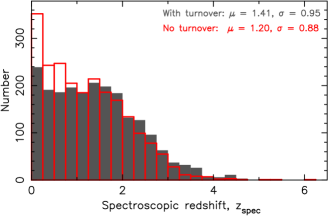
Figure 4: The redshift distributions of the radio sources with and without turnovers in their SEDs. A Kolmogorov-Smirnov test gives a probability of $7.86\times 10^{-9}$ of the sources being drawn from the same sample.

From the remaining features we again shortlisted those in Table LABEL:intersect_all with $n_{\text{int}}\geq 1001$. Testing this, we see that all algorithms gave a significant improvement in the regression coefficient over the previous models, although the other metrics show that these still have little predictive power.

By removing the need for the SEDs to be fit by either a polynomial or the Snellen et al. function significantly increases the sample sizes, by utilising only the fluxes in the model (Table LABEL:intersect_all). This is analogous to the NIR–optical–UV model (Sect. 4.2.1) and, like the one-hot encoded sample, this outperforms both the poly and snellen samples. From Table 4, we see that the samples with $n_{\text{int}}\geq 716$ and $n_{\text{int}}\geq 549$ give the best results, with no difference between the two models within the $1\sigma$ uncertainties, despite the significant drop in sample sizes from $n_{\text{int}}\geq 2037$. This suggests that the low frequency flux densities ($S_{\text{70 MHz}}$ & $S_{\text{150 MHz}}$) may be important features in the prediction of photometric redshifts. We therefore, also tested the ohe sample including the next numerous feature, $S_{\text{150 MHz}}$, giving $n_{\text{int}}\geq 351$. Although the numbers are small, just 71 validation sources, we see further improvement in the statistics. However, within the larger $1\sigma$ uncertainties the results are consistent with the $n_{\text{int}}\geq 1001$ ohe results for all of the machine learning algorithms. We would therefore err towards the $r\approx 0.39$ given by the ANN trials as being representative. There is also the possibility that the relatively good statistics are due to the much smaller test sample. In any case, these still fall far short of being able to provide photometric redshift predictions (Fig. 5).

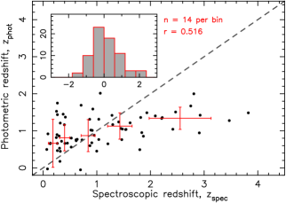
Figure 5: The photometric versus the spectroscopic redshift for the 71 validation sources for a single run of the SVR algorithm on the ohe $n_{\text{int}}\geq 351$ sample. The binning is for an equal number of sources in each bin with the error bars showing $\pm 1\sigma$. The broken line shows $z_{\text{phot}}=z_{\text{spec}}$ and the inset the distribution of $\Delta z$.

Lastly, the fact that the ohe and flux samples provide better models than the poly and snellen samples suggests there may be something wrong with the fitting. This is a possibility since the fits were performed on heterogeneously sampled data, with the requirement of at least three photometry measurements (9833 sources) for the polynomial fit and at least five for the Snellen et al. fit (5604 sources, of which not all could be fit). This can lead to clear under-sampling of some SEDs, possibly giving unrepresentative fits, although raising this minimum requirement drastically cut the sample sizes still further (Fig. 6).

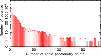
Figure 6: The distribution of the number of radio photometry measurements.

Whether or not a fit is present does, however, seem to provide a useful feature (the ohe sample) and so with better sampling of the SEDs, giving more accurate measurements of the fit parameters, these may yet prove to be useful features.

4.1.3 Effectiveness of the machine learning

Although the results are indicative of the radio data being ineffective in providing a redshift prediction model, we do see some quite strong variation across the models (e.g. the regression coefficient ranging from $r\approx 0.06$ to 0.46, Table 4). While the numbers are small and it is not known if the most numerous features are the most optimal (Table LABEL:intersect_all), we can test if the algorithms are at least partially effective in predicting photometric redshifts.

For this, we select the $n_{\text{int}}\geq 1001$ ohe sample, since this yields some of the highest values of $r$ for all algorithms, while providing a relatively large sample. For each algorithm we train on progressively fewer sources and validate on another 100. That is, training on 900, 800, …, 100, 50, 20,10 sources, randomly selected for each of the 100 trials. From the results (Fig. 7),

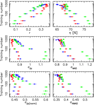
Figure 7: The results for the kNN (red), SVR (blue) and DTR (green) one-hot encoded models ($n_{\text{int}}\geq 1001$) based on different training sample sizes. Note that for clarity the error bars show the standard error about the mean.

we see that all models are indicative of the algorithms being effective, with an increase in $r$ with the training size along with a decrease in the spread in $\Delta z$. Note, however, that the figure shows the standard errors, since the $\pm 1\sigma$ ranges exceed the abscissa ranges. For instance, for the SVR model $r=0.11\pm 0.18$ training on 10 sources and $0.33\pm 0.08$ training on 900. So while the mean values appear to improve with the training sample size, the uncertainties are too large to state this definitively.

4.2 NIR–optical–UV photometric redshifts

4.2.1 Training and validation

We also tested the predictive power of the machine learning models, using the NIR–optical–UV photometry, which has proven successful in training and validation upon sources from a single dataset (i.e. the SDSS, e.g. Bovy et al. 2012; Brescia et al. 2013), as well as training on one dataset and validating upon another (i.e. the SDSS on radio-selected quasars from external catalogues, Curran 2020; Curran et al. 2021). Of the Milliquas radio sources, there were 12 503 which had all of the $W2,W1,z,i,r,g,u,NUV,FUV$ magnitudes, which we used directly as features.

Table 5: The mean values $\pm 1\sigma$ of 100 trials of the machine learning algorithms using the NIR–optical–UV magnitudes (2501 validation sources).

		Un-normalised			Normalised
	$r$	$\mu_{\Delta z}$	$\sigma_{\Delta z}$	$\sigma_{\text{MAD}}$	$\mu_{\Delta z(\text{norm})}$	$\sigma_{\Delta z(\text{norm})}$	$\sigma_{\text{NMAD}}$	$\eta$
kNN	$0.911\pm 0.006$	$0.019\pm 0.008$	$0.308\pm 0.011$	$0.141\pm 0.005$	$-0.013\pm 0.004$	$0.143\pm 0.004$	$0.077\pm 0.002$	$17.7\pm 0.7$ %
SVR	$0.913\pm 0.005$	$0.016\pm 0.006$	$0.283\pm 0.009$	$0.149\pm 0.004$	$-0.008\pm 0.003$	$0.142\pm 0.043$	$0.089\pm 0.002$	$17.0\pm 0.8$%
DTR	$0.858\pm 0.009$	$0.002\pm 0.009$	$0.387\pm 0.013$	$0.170\pm 0.007$	$-0.022\pm 0.004$	$0.204\pm 0.011$	$0.091\pm 0.003$	$22.6\pm 0.8$%
ANN	$0.944\pm 0.003$	$-0.005\pm 0.030$	$0.249\pm 0.006$	$0.115\pm 0.012$	$-0.016\pm 0.018$	$0.124\pm 0.006$	$0.066\pm 0.009$	$11.6\pm 1.4$%

From Table 5, we see that all models are successful, with the ANN (Fig. 8) being comparable with the SDSS model of Curran et al. (2021).

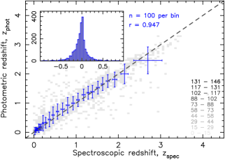
Figure 8: An instance of the photometric redshift predictions from the NIR–optical–UV photometry versus the spectroscopic redshift for the 2501 Milliquas validation sources, trained upon the other 10 002 Milliquas radio sources. The grey-scale shows the source distribution with the key to the bottom right showing the number within each pixel. Here $\mu_{\Delta z}=-0.03$, $\sigma_{\Delta z}=0.24$, $\sigma_{\text{MAD}}=0.11$, $\mu_{\Delta z(\text{norm})}=-0.03$, $\sigma_{\Delta z(\text{norm})}=0.13$, $\sigma_{\text{NMAD}}=0.06$ and $\eta=11$%.

That is, using the NIR–optical–UV features appears to perform significantly better than the radio selected features. This, however, is based upon a much larger sample for which the training may be more comprehensive. In order to test whether a larger training sample was the reason for the NIR–optical–UV model’s superiority, we selected a similar number of sources (1000) at random from those with the complete $W2,W1,z,i,r,g,u,NUV,FUV$ photometry. Again, using the 80:20 training–validation split, we would train on 800 of the sources and validate on the remaining 200, before selecting another 1000 sources at random and repeating until 100 trials were complete.

Table 6: The results of the machine learning algorithms for a sample of 1000 unique sources selected at random from the Milliquas sample. We run each algorithm 100 times, randomising the 1000 sources each time and so quote the mean values, with $\pm 1\sigma$.

		Un-normalised			Normalised
	$r$	$\mu_{\Delta z}$	$\sigma_{\Delta z}$	$\sigma_{\text{MAD}}$	$\mu_{\Delta z(\text{norm})}$	$\sigma_{\Delta z(\text{norm})}$	$\sigma_{\text{NMAD}}$	$\eta$
kNN	$0.87\pm 0.03$	$0.03\pm 0.03$	$0.37\pm 0.05$	$0.22\pm 0.02$	$-0.02\pm 0.01$	$0.17\pm 0.02$	$0.12\pm 0.01$	$29.0\pm 3.1$%
SVR	$0.89\pm 0.03$	$0.01\pm 0.03$	$0.33\pm 0.05$	$0.20\pm 0.02$	$-0.02\pm 0.01$	$0.17\pm 0.02$	$0.12\pm 0.01$	$25.3\pm 3.1$%
DTR	$0.78\pm 0.04$	$0.01\pm 0.04$	$0.46\pm 0.04$	$0.29\pm 0.04$	$-0.04\pm 0.02$	$0.23\pm 0.03$	$0.16\pm 0.02$	$38.3\pm 3.7$%
ANN	$0.90\pm 0.03$	$0.00\pm 0.09$	$0.33\pm 0.04$	$0.20\pm 0.03$	$-0.02\pm 0.04$	$0.16\pm 0.03$	$0.12\pm 0.02$	$24.1\pm 5.3$%

The results are summarised in Table 6, from which we see the NIR–optical–UV model still provides accurate photometric redshifts, thus confirming that the $W2,W1,z,i,r,g,u,NUV,FUV$ photometry provide superior features to those in the radio band.

4.2.2 SDSS training of Milliquas sources

We also tested the prediction of the redshifts of the Milliquas sources, based upon our SDSS model. That is, using the 71 267 of the 100 337 SDSS QSOs with the full NIR–optical–UV photometry (Curran et al., 2021) to train a model which we then validate on the Milliquas radio sources. This frees up the Milliquas data from training, giving photometric redshifts for all 12 503 sources with the full magnitude complement and, from

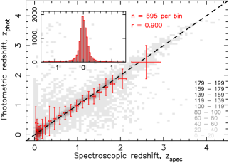
Figure 9: Validation of Milliquas redshifts predicted from an NIR–optical–UV photometry model trained on the SDSS sample of Curran et al. (2021). Here $n=12\,503$, $\mu_{\Delta z}=0.00$, $\sigma_{\Delta z}=0.33$, $\sigma_{\text{MAD}}=0.14$, $\mu_{\Delta z(\text{norm})}=-0.02$, $\sigma_{\Delta z(\text{norm})}=0.23$, $\sigma_{\text{NMAD}}=0.08$ and $\eta=19$%.

Fig. 9, we see that the SDSS provides a good model with metrics close to that of other external datasets validated upon the SDSS model (Curran et al. 2021, see also Sect. 4.2.3). This is despite quite different distributions in the magnitudes between all of the tested data (Fig. 10).

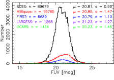
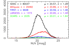
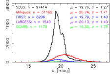
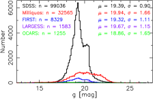
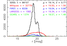
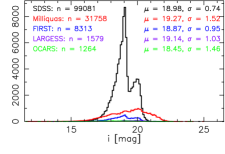
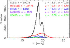
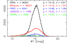
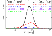
Figure 10: The distribution of each of the magnitudes for the sample compared to the SDSS and our three radio selected catalogues (see Sect. 4.2.3).

Compared to training the model on the Milliquas sample (Fig. 8), we see the majority of the scatter to occur at $z\sim 0$. We have previously noted the lower redshifts to be problematic in our SDSS sample, probably due to the relatively unreliable FUV fluxes which are important in utilising the $\lambda=1216$ Å Lyman-break in the model (Curran et al., 2021). From the “magnitude profiles” of the datasets (Fig. 11),

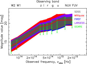
Figure 11: The “magnitude profiles” of the various databases, where the coloured bands show the mean magnitude $\pm 1\sigma$ (Fig. 10). For clarity, OCARS (see Sect. 4.2.3) is shown as error bars and the mean magnitudes from the Milliquas sources have also been over-plotted as a line.

we confirm that the Milliquas magnitudes differ from those of the SDSS, with the former being flatter across $NUV$ and $FUV$.

4.2.3 Milliquas training of radio selected sources

A major issue with training a model using SDSS photometry is that these are restricted to the northern sky only, whereas the SKA and its pathfinders will survey the southern sky. In Curran et al. (2021) we suggested that SkyMapper (Wolf et al., 2018), which will survey the southern sky in the $u,v,g,r,i,z$ bands, could provide the photometry for the SKA sources. Until the SkyMapper data become generally available, we can test if alternative datasets to the SDSS are viable using the Milliquas data. Although these are also predominately located in the northern sky (see Sect. 4.3), their magnitude distributions are quite distinct from those of the SDSS (Fig. 10).

As discussed in Curran & Moss (2019), large catalogues of radio sources with spectroscopic redshifts are rare and so we use the same samples as previously (Curran et al., 2021):

1. The Faint Images of the Radio Sky at Twenty-Centimeters (FIRST, Becker et al. 1995; White et al. 1997) sample. Of the 18 273 sources with redshifts from the SDSS DR14 QSOs (Pâris et al., 2018) 9016 are classified in NED as QSOs.

2. The Large Area Radio Galaxy Evolution Spectroscopic Survey (LARGESS). Of the 10 685 sources with optical redshifts (Ching et al., 2017) 1608 are classified in NED as QSOs.

3. The Optical Characteristics of Astrometric Radio Sources (OCARS) catalogue of Very Long Baseline Interferometry (VLBI) astrometry sources (Ma et al., 2009; Malkin, 2018). Of the 7800 sources, 3151 are classified in NED as QSOs.

In Fig. 12, we show the predicted redshifts from the validation of the sources in the above catalogues trained upon the Milliquas radio sources.

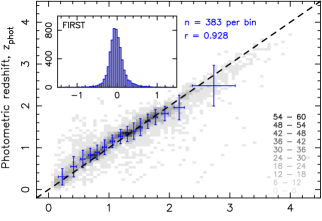
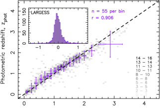
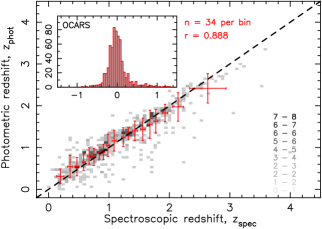
Figure 12: Validation of the redshifts from the three external radio-selected databases from a model trained on the Milliquas sources. Top: FIRST – $n=6129$, $\mu_{\Delta z}=-0.01$, $\sigma_{\Delta z}=0.25$, $\sigma_{\text{MAD}}=0.16$, $\mu_{\Delta z(\text{norm})}=-0.02$, $\sigma_{\Delta z(\text{norm})}=0.11$, $\sigma_{\text{NMAD}}=0.07$ and $\eta=11\%$. Middle: LARGESS – $n=1046$, $\sigma_{\Delta z}=0.30$, $\mu_{\Delta z}=0.0$, $\sigma_{\text{MAD}}=0.16$, $\mu_{\Delta z(\text{norm})}=-0.02$, $\sigma_{\Delta z(\text{norm})}=0.12$, $\sigma_{\text{NMAD}}=0.08$ and $\eta=10$%. Bottom: OCARS – $n=649$, $\mu_{\Delta z}=0.02$, $\sigma_{\Delta z}=0.31$, $\sigma_{\text{MAD}}=0.16$, $\mu_{\Delta z(\text{norm})}=-0.01$, $\sigma_{\Delta z(\text{norm})}=0.11$, $\sigma_{\text{NMAD}}=0.08$ and $\eta=18$%.

The results are largely indistinguishable from the SDSS training (Table 7), even though the SDSS sample is significantly larger and we had previously used the colours, rather than magnitudes, as features.

Table 7: Comparison of the radio catalogue predictions from the SDSS (71 267 QSOs, Curran et al. 2021) and Milliquas (44 119 quasars) magnitudes.

Sample	$r$		$\sigma_{\Delta z}$		$\sigma_{\text{MAD}}$		$\sigma_{\Delta z(\text{norm})}$		$\sigma_{\text{NMAD}}$
	SDSS	Milliquas	SDSS	Milliquas	SDSS	Milliquas	SDSS	Milliquas	SDSS	Milliquas
FIRST	0.93	0.93	0.245	0.248	0.102	0.158	0.110	0.111	0.048	0.072
LARGESS	0.91	0.91	0.297	0.392	0.123	0.163	0.123	0.120	0.057	0.075
OCARS	0.85	0.89	0.371	0.307	0.132	0.164	0.170	0.131	0.063	0.076

4.3 Imputation of missing data

As mentioned in Sect. 4.2.1, only 12 503 of the 44 119 Milliquas sources have the full magnitude complement. Like the OCARS sources, much of this can be attributed to Milliquas covering the whole sky, whereas the SDSS

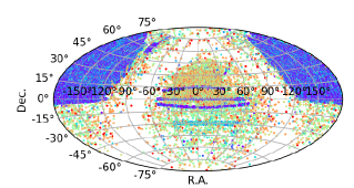
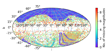
Figure 13: The sky distribution of the Milliquas radio sources in equatorial (left) and Galactic (right) coordinates, colour coded by the number of missing magnitudes per source.

is limited to the northern sky (Fig. 13, left). However, we also see that a significant amount of GALEX photometry is missing (Table 8).

Table 8: The number of missing magnitude measurements in each of the bands for the Milliquas sources.

$FUV$	$NUV$	$u$	$g$	$r$	$i$	$z$	$W1$	$W2$
24 365	14 646	12 968	11 565	11 351	12 372	12 655	5903	6047

Given the similarity between the distribution of missing magnitudes in Galactic coordinates (Fig. 13, right) and the $NUV\cap FUV\cap$ SDSS distribution (Bianchi et al., 2014), we, again, attribute this to the sky coverage.

In combination with the missing WISE magnitudes, this means that we can only predict redshifts for 28% of the sample. We therefore explore the possibility of replacing the missing values (data imputation, e.g. Luken et al. 2021; Gibson et al. 2022), via the best two performing methods found by Curran (2022):

1. Simple imputation: The missing feature is replaced with a constant, either the mean, median or most frequently occuring value. All of these methods were effective for training and validation upon the SDSS sample, in particular replacing the missing magnitudes with the maximum value for that band (analogous to assuming that the missing magnitude is at the detection limit, Carvajal et al. 2021). This method, however, was not effective in applying the SDSS model to the imputed radio samples.

2. Multivariate (multiple) imputation: Machine learning is used to estimate the missing values from the other features. Although, along with the other model-based methods which were tested, this is not as good a performer as simple imputation when validating upon the same dataset, it did produce the best results when used to impute the missing values in the three radio samples, which were trained by the SDSS model. If the number of missing magnitudes was limited to two per source high quality predictions were retained (Curran, 2022).

As previously, for training and validating on the same dataset, we find replacing the missing magnitudes with the maximum value for that band

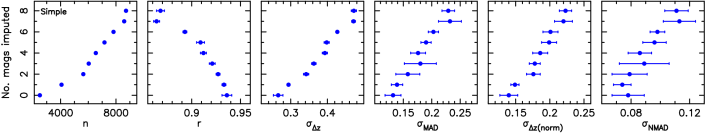
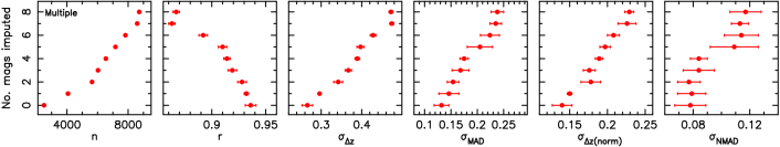
Figure 14: The performance of the ANN for different numbers of imputed magnitudes per source using simple (top) and multivariate (bottom) imputation for self-training with the Milliquas sources. The 20% self-validation number ranges from 2501 (no imputed magnitudes) to 8719 (eight imputed). The error bars show the $\pm 1\sigma$ from the mean of 10 trials, each with a randomly selected training and validation sub-sample.

to be an effective imputation strategy (Fig. 14, top), with the results indistinguishable from the multivariate imputation (Fig. 14, bottom). However, due to the majority of the sample being used for training, this only yields predictions for a small portion of the sample. Therefore in Fig. 15 we show the results of validating upon the imputed Milliquas data trained on the SDSS data (see Sect. 4.2.2).

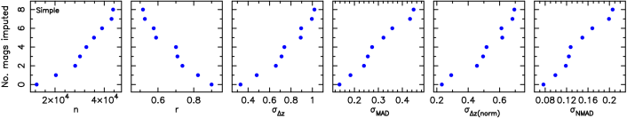
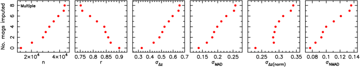
Figure 15: The performance of the ANN for different numbers of imputed magnitudes per each of the Milliquas sources, using simple (top) and multivariate (bottom) imputation, predicted from the SDSS model. The number of sources ranges from 12 503 (no imputed magnitudes) to 43 595 (99% of the sample for eight imputed).

From this, we see that, unlike when self-training, the multiple imputation significantly outperforms the simple imputation. From the metrics it is not clear what a reasonable limit to the number of imputed magnitudes should be, although the regression coefficient (and perhaps NMAD) suggests up to four, while the normalised standard deviation suggests that this may be best limited to one.

Replacing the missing data for sources with only one absent magnitude, gives only a moderate increase in sample size (to 20 332) and Curran (2022) suggests that up to two is reasonable when applying the SDSS model to external datasets. Therefore in Fig. 16, we show the results for both up to two and four imputed magnitudes per source.

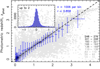
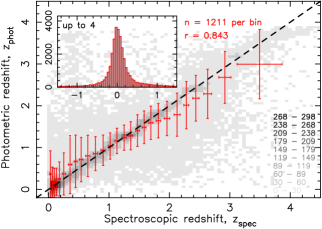
Figure 16: The photometric versus the spectroscopic redshift for the Milliquas radio sources from the SDSS model (Fig. 9), but where up to two (top) and four (bottom) missing values per source are imputed. In the top panel, $n=28\,173$, $\sigma_{\Delta z}=0.482$, $\sigma_{\text{MAD}}=0.182$, $\sigma_{\Delta z(\text{norm})}=0.283$, $\sigma_{\text{NMAD}}=0.093$ and $\eta=24.5$%. In the bottom panel, $n=32\,698$, $\sigma_{\Delta z}=0.526$, $\sigma_{\text{MAD}}=0.198$, $\sigma_{\Delta z(\text{norm})}=0.290$ $\sigma_{\text{NMAD}}=1.00$ and $\eta=26.8$%.

.

Compared to the 12 503 non-imputed sources (Fig. 9), the binned data clearly shows in increasing inaccuracy in the photometric redshift predictions, with the outlier fraction climbing from $\eta=19.0$% for 12 504 sources to $24.5$% for 28 173 and $26.8$% for 32 698. Thus, the number of sources which can be fit by imputing up to four features per sources is 2.6 times that of the sources with all of the magnitudes (up from 28% to 74% of the sample), at the expense of 1.4 times as many outliers.

Given the effectiveness of the imputation of the missing magnitudes, we also explored the possibility of imputing the missing radio data, adding much-needed training data (cf. Table LABEL:intersect_all). In order to minimise the number of sources with many missing features and utilise numerical values only, we considered only the flux sample. Even so, unlike the NIR–optical–UV case, the vast majority of sources still have a large number of missing features (Fig. 17).

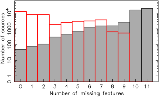
Figure 17: The number of missing radio flux measurements (filled histogram) and the number of missing magnitudes (unfilled) for the 41 119 Milliquas quasars.

For example, imputing up to two missing values per source only yields 239 sources, with the imputation of six required to reach 2990. This nearly doubles (to 5957) if we exclude the 15 and 20 GHz flux densities, although, perhaps unsurprisingly, there is no improvement in the machine learning results ($r\approx 0.29,\,\sigma_{\Delta z}\approx 0.81,\,\sigma_{\text{MAD}}\approx 0.82,\,\sigma_{\Delta z(\text{norm})}\approx 0.42,\,\sigma_{\text{NMAD}}\approx 0.37$ and $\eta\approx 70$%). We therefore conclude that, due to the majority of sources being dominated by a large number of missing features, data imputation is not (yet) useful for replacing the missing radio data.

5 Discussion

5.1 Radio photometric redshifts

Despite extensive testing, for which the main models are described in Sect. 4.1, we could not find a machine learning model or artificial neutral network which could accurately predict the redshifts of the sources based upon features in the radio SED alone. Although the training sample is significantly smaller, $\approx 1000$ sources compared to $\approx 10\,000$ for the Milliquas validation sample, the NIR–optical–UV photometry can still produce accurate predictions for the smaller sample size. It should be noted, however, that these 1000 sources have the full NIR–optical–UV photometry, comprising nine features each, while the radio sample has just six features (including the presence of a turnover in the SED, Table LABEL:intersect_all). We also find circumstantial evidence that a much larger radio photometric sample may yet prove useful (Fig. 7).

Using the radio flux densities at different frequencies is analogous to the magnitudes in the prediction of redshifts, although from Fig. 2 it is apparent that the radio photometry may be steeply flux limited, a clear example being the abrupt decrease in sources with $S_{1.4~{}\text{GHz}}\stackrel{{\scriptstyle<}}{{{}_{\sim}}}10^{-3}$ Jy. Over a heterogeneously sampled radio SED this could cause some frequencies to drop out of the training model before others, causing uneven sampling of the sources. This may also be responsible for the bimodal distribution in the flux densities, which are not correlated strongly with redshift (e.g. $S_{\text{150 MHz}}$, Table 2). This of course could also be an issue for the NIR–optical–UV magnitudes, but each of the these bands are dominated by a single survey (WISE, SDSS & GALEX) and the SED as a whole is dominated by the SDSS.

In Fig. 18, we see that, like the SDSS and FIRST samples, Milliquas does appear to suffer from a flux limitation.

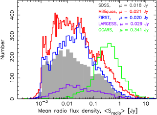
Figure 18: The mean radio flux densities of the QSOs/quasars in the SDSS, Milliquas, FIRST, LARGESS and OCARS with measured $\leq 10$ GHz flux densities (updated from Curran et al. 2021). In order to fit within a similar range, the Milliquas binning is four times finer and the FIRST twice as fine as for the other samples.

This is least apparent for the OCARS fluxes, probably due to the much higher brightness of these sources. The lack of apparent flux limitation suggests that OCARS may provide a better model for the radio photometric redshift. Testing this, we find the results to also be disappointing, although the sample significantly smaller than the Milliquas (see Appendix A).

We note that direct comparison of the radio properties with the NIR–optical–UV magnitudes may not be justified, as the latter spans over three observing bands, although arguably the 70 MHz – 20 GHz is also over several bands, even if unevenly sampled. Other previous studies have also failed to find a photometric redshift (Majic & Curran, 2015; Norris et al., 2019), a possible explanation being the relatively featureless radio SEDs: While the value of turnover frequency may be dictated by intrinsic source properties such as the extent of the radio emission (e.g. O’Dea 1998; Fanti 2000; Orienti et al. 2006) and the electron density (de Vries et al., 1997; Curran et al., 2019), the observed wavelengths of the $\lambda\sim 1~{}\mu$m inflection in the NIR and $\lambda=1216$ Å Lyman-break in the UV are two features which are dependent on the redshift.

5.2 NIR–optical–UV photometric redshifts

Although a redshift prediction from radio data is not yet possible, we find that the redshifts of sources in the external three radio catalogues can be accurately predicted from a model trained on the Milliquas radio sources using their NIR–optical–UV magnitudes. This was previously shown to be the case for training on a sample of SDSS QSOs (Curran et al., 2021) and, the fact that the Milliquas give very similar metrics (Sect. 4.2.2), gives us confidence that SkyMapper will be able to provide a model for the southern sources, not accessible to the SDSS (see Sect. 4.3).

This similarity in the results of the Milliquas and SDSS models arises despite the very different magnitude (Fig. 10) and redshift (Fig. 19) distributions.

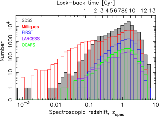
Figure 19: The redshift distributions of the different samples.

From the latter, we see that the Milliquas radio sources sample the low redshifts ($z\stackrel{{\scriptstyle<}}{{{}_{\sim}}}0.1$) significantly more comprehensively than our SDSS training sample. This may result in the Milliquas providing a better model at low redshift. Examining this, in Fig. 20

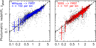
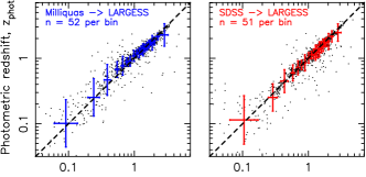
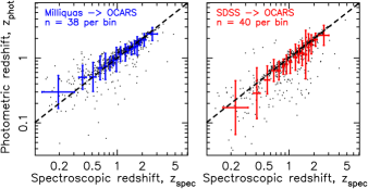
Figure 20: Comparison of the Milliquas (left) and SDSS (right) models emphasising the low redshifts. Top: Redshift predictions for the FIRST QSOs versus the measured redshifts. Middle: LARGESS QSOs. Bottom: OCARS quasars. The bin sizes differ slightly as the very few $z_{\text{phot}}<0$ predictions are excluded.

we see that any improvement at low redshift is most pronounced for the FIRST predictions at $z\stackrel{{\scriptstyle<}}{{{}_{\sim}}}0.2$. We also see that overall the Milliquas does appear to provide a better model of the OCARS redshift predictions. From the statistics (Table 7), the Milliquas does rate significantly better according to the regression coefficient and standard deviations, although the median absolute deviations are poorer to a similar degree.

6 Conclusions

In order to expand upon our previous work in using machine learning and artificial neural networks to obtain the redshifts of radio sources, we have explored using the Million Quasars Catalogue. From this, there are 44 495 sources classed as radio sources which have a spectroscopic redshift. We were able to match 44 119 of these in NED and obtain the available photometry, spanning the radio to ultraviolet bands. The aim was to obtain a large sample of quasars with which to test for potential redshift prediction from the radio spectrum alone. For these we test:

• Peaked spectrum sources only, where the turnover parameters are included as features.

• All of the sources, by one-hot encoding the presence of a turnover in the spectrum as a feature.

• All of the sources, using only the flux densities as features.

We find from these models that the radio spectrum has little predictive power. One possibility is the trade-off between sample size and number of features, although testing the NIR–optical–UV model on a similar size sample shows a sample of $\sim 1000$ to still be useful. However, it may still be possible for a much larger sample to yield positive results from the largely featureless radio SEDs, especially if the rare features (e.g. the 70 & 150 MHz fluxes) prove to be critical, and we do find marginal evidence for the predictive power of the models improving with training sample size.

Another cause of the poor performance may be the flux limitation, where the sample is abruptly truncated at flux densities of $S\stackrel{{\scriptstyle<}}{{{}_{\sim}}}10^{-3}$ Jy. For fluxes compiled from several disparate sources, this would introduce non-uniform sampling of the SEDs, effectively scrambling the data. This flux limitation is not apparent for one of our test samples, the OCARS catalogue of VLBI astrometry sources, probably due to the much higher flux densities. Again, however, this has little predictive power although the amount of available training data is significantly smaller.

We also explore how the NIR–optical–UV photometry of the 12 503 Milliquas radio sources, with the full $W2,W1,z,i,r,g,u,NUV,FUV$ complement, compares to that of the SDSS in providing a model with which to predict of the redshifts of radio selected samples:

1. Despite differences in their distributions, the same NIR–optical–UV photometry, which has a proven success in yielding photometric redshifts for SDSS QSOs, appears to work equally well in the training and validation of the Milliquas radio sources. Training on 10 002 and validating on 2501 of the sample, gives an outlier fraction of $\eta=12\%$.

2. Training a model on the SDSS sample (Curran et al., 2021) and validating on the 12 503 Milliquas sources is successful, with an outlier fraction of $\eta=19\%$.

3. Training a model on the Milliquas sample and validating on three external catalogues of radio selected sources yields outlier fractions of $\eta\leq 18$% and spreads in $\Delta z$ which are indistinguishable from training on the SDSS data. This transferability gives us confidence that future SkyMapper measurements of the $u,v,g,r,i,z$ bands in the southern sky can be combined with the NIR and UV photometry to give a reliable model to yield photometric redshifts of sources detected with the SKA.

4. In some cases Milliquas outperforms the SDSS model in the validation of the external radio sources at low redshifts due to better sampling. This suggests that the results from different training models may be reliably combined according to where they have the best redshift coverage.

5. As per the SDSS data (Curran, 2022), machine learning can be used to impute the missing data with the replacement of up to four magnitudes per source, increasing the number of sources to 32 698 (73% of the sample) at the cost of the outlier fraction rising to 27%.

To conclude, although a radio photometric redshift remains elusive, the fact that the same optical bands of a distinct dataset can provide an accurate model promises great potential in using machine learning to obtain the redshifts of the large number of sources to be discovered in forthcoming surveys.

Data availability

Data and training models available on request.

Appendix A

Radio photometric redshifts from OCARS

In this appendix we test the potential of using the OCARS quasars to find a radio photometric redshift model. In Fig. 21, we show the redshift distributions of

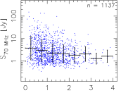
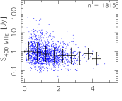
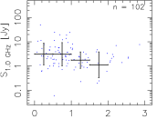
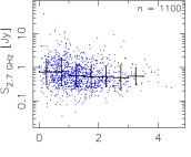
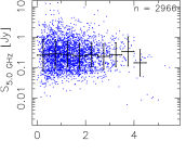
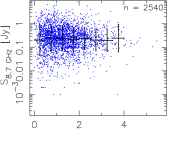
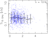
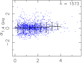
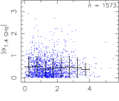
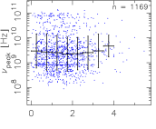
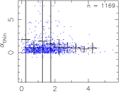
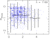
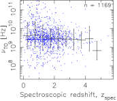
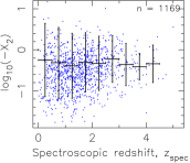
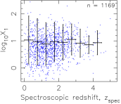
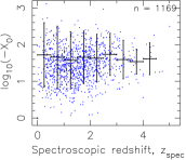
Figure 21: As Fig. 2 but for the OCARS quasars.

the features (Sect. 2.3.1), from which the steep cut-off at lower flux densities, evident for the Milliquas QSOS, appears to be missing (cf. Fig. 2). In addition to having higher fluxes, the correlations can also be quite different (Table 9).

Table 9: The feature redshift correlations for the OCARS quasars (Fig. 21).

Feature	$n$	$P(\tau)$	$Z(\tau)$
$\log_{10}S_{\text{70 MHz}}$	1137	$2.69\times 10^{-11}$	$6.67\sigma$
$\log_{10}S_{\text{150 MHz}}$	800	$2.69\times 10^{-15}$	$7.91\sigma$
$\log_{10}S_{\text{400 MHz}}$	1815	$7.21\times 10^{-16}$	$8.07\sigma$
$\log_{10}S_{\text{700 MHz}}$	210	0.030	$2.17\sigma$
$\log_{10}S_{\text{1.0 GHz}}$	102	0.084	$1.73\sigma$
$\log_{10}S_{\text{1.4 GHz}}$	2908	$4.48\times 10^{-3}$	$2.82\sigma$
$\log_{10}S_{\text{2.7 GHz}}$	1100	$7.65\times 10^{-9}$	$5.78\sigma$
$\log_{10}S_{\text{5.0 GHz}}$	2966	0.047	$1.99\sigma$
$\log_{10}S_{\text{8.7 GHz}}$	2540	0.039	$2.07\sigma$
$\log_{10}S_{\text{15 GHz}}$	1016	$5.80\times 10^{-4}$	$3.43\sigma$
$\log_{10}S_{\text{20 GHz}}$	1470	$3.35\times 10^{-11}$	$6.63\sigma$
$\alpha_{1.4~{}\text{GHz}}$	1573	0.032	$2.13\sigma$
$|\alpha_{1.4~{}\text{GHz}}|$	1573	0.038	$2.07\sigma$
$\log_{10}\nu_{\text{peak}}$	1169	0.915	$0.11\sigma$
$\log_{10}S_{\text{peak}}$	1169	0.113	$1.59\sigma$
$\alpha_{\text{thin}}$	1169	0.423	$0.80\sigma$
$\alpha_{\text{thick}}$	1169	0.156	$1.42\sigma$
$\log_{10}\nu_{\text{TO}}$	1169	$5.57\times 10^{-5}$	$4.01\sigma$
$\log_{10}S_{\text{TO}}$	1169	$2.43\times 10^{-4}$	$3.65\sigma$
$\log_{10}(-X_{2})$	1169	$6.54\times 10^{-3}$	$2.72\sigma$
$\log_{10}X_{1}$	1169	0.012	$2.50\sigma$
$\log_{10}(-X_{0})$	1169	0.022	$2.30\sigma$

Specifically the strong redshift correlation with $\log_{10}S_{\text{150 MHz}}$, $\log_{10}S_{\text{15 GHz}}$, $\log_{10}S_{\text{20 GHz}}$, $\log_{10}\nu_{\text{TO}}$ and $\log_{10}S_{\text{TO}}$, missing for the Milliquas sources (Table 2), but the lack of strong correlation with $\log_{10}S_{\text{700 MHz}}$, $\log_{10}S_{\text{1.0 GHz}}$ and $\log_{10}S_{\text{1.4 GHz}}$.

In Table 10, we also see that the distribution of the feature counts is quite different from the Milliquas sources (Table LABEL:intersect_all),

Table 10: Features common to the sources in (column) descending order of sample size (Table 9).

Feature	$n$	$n_{\text{int}}$	Feature	$n$	$n_{\text{int}}$
$\log_{10}S_{\text{5.0 GHz}}$	2966	2966	Snellen et al. fit	1169	311
$\log_{10}S_{\text{1.4 GHz}}$	2908	2772	$\log_{10}S_{\text{70 GHz}}$	1137	89
$\log_{10}S_{\text{8.7 GHz}}$	2540	2281	$\log_{10}S_{\text{2.7 GHz}}$	1100	69
$\log_{10}S_{\text{400 MHz}}$	1815	1464	$\log_{10}S_{\text{15 GHz}}$	1016	55
$\alpha_{1.4~{}\text{GHz}}$	1573	706	$\log_{10}S_{\text{150 MHz}}$	800	30
$\log_{10}S_{\text{20 GHz}}$	1470	458	$\log_{10}S_{\text{700 MHz}}$	210	20
Polynomial fit	1169	311	$\log_{10}S_{\text{1.0 GHz}}$	102	12

although the inclusion of all features still results in a total sample size of just 12. Again, prioritising by the most overlapping features, while still retaining a sufficient number of sources, we test various machine learning models, equivalent to those tested for the Milliquas QSOs (Sect. 4.1).

Table 11: Results from the validation of the models (Sect. 4.1), based upon the OCARS features (Table 10).

		Un-normalised			Normalised
	$r$	$\mu_{\Delta z}$	$\sigma_{\Delta z}$	$\sigma_{\text{MAD}}$	$\mu_{\Delta z(\text{norm})}$	$\sigma_{\Delta z(\text{norm})}$	$\sigma_{\text{NMAD}}$	$\eta$
$n_{\text{int}}\geq 311$ of the poly sample (63 validation sources)
kNN	$0.19\pm 0.12$	$-0.04\pm 0.11$	$0.77\pm 0.07$	$0.75\pm 0.11$	$-0.12\pm 0.05$	$0.38\pm 0.04$	$0.31\pm 0.05$	$60.5\pm 6.0$%
SVR	$0.20\pm 0.10$	$0.03\pm 0.10$	$0.77\pm 0.07$	$0.71\pm 0.12$	$-0.09\pm 0.05$	$0.37\pm 0.03$	$0.29\pm 0.05$	$60.1\pm 5.9$%
DTR	$0.09\pm 0.12$	$-0.03\pm 0.12$	$0.86\pm 0.08$	$0.79\pm 0.13$	$-0.12\pm 0.06$	$0.42\pm 0.05$	$0.32\pm 0.05$	$63.3\pm 6.4$%
ANN	$0.03\pm 0.09$	$-0.03\pm 0.32$	$0.85\pm 0.05$	$0.84\pm 0.13$	$-0.10\pm 0.14$	$0.38\pm 0.05$	$0.34\pm 0.06$	$64.9\pm 7.5$%
$n_{\text{int}}\geq 311$ of the snellen sample (63 validation sources)
kNN	$0.10\pm 0.10$	$0.00\pm 0.12$	$0.79\pm 0.06$	$0.77\pm 0.11$	$-0.11\pm 0.06$	$0.38\pm 0.04$	$0.31\pm 0.04$	$63.1\pm 5.8$%
SVR	$0.09\pm 0.11$	$0.04\pm 0.12$	$0.80\pm 0.06$	$0.80\pm 0.11$	$-0.09\pm 0.06$	$0.39\pm 0.04$	$0.32\pm 0.04$	$65.0\pm 5.2$%
DTR	$0.00\pm 0.11$	$-0.01\pm 0.13$	$0.89\pm 0.08$	$0.86\pm 0.12$	$-0.12\pm 0.06$	$0.44\pm 0.06$	$0.35\pm 0.05$	$66.7\pm 5.5$%
ANN	$0.01\pm 0.07$	$0.03\pm 0.27$	$0.86\pm 0.04$	$0.91\pm 0.08$	$-0.08\pm 0.12$	$0.39\pm 0.04$	$0.36\pm 0.04$	$68.1\pm 4.5$%
$n_{\text{int}}\geq 706$ of the ohe sample (142 validation sources)
kNN	$0.28\pm 0.06$	$0.01\pm 0.07$	$0.80\pm 0.05$	$0.79\pm 0.07$	$-0.10\pm 0.03$	$0.38\pm 0.03$	$0.32\pm 0.03$	$61.7\pm 3.6\%$
SVR	$0.21\pm 0.07$	$0.06\pm 0.08$	$0.86\pm 0.06$	$0.80\pm 0.07$	$-0.08\pm 0.03$	$0.41\pm 0.04$	$0.33\pm 0.03$	$63.4\pm 3.5$%
DTR	$0.19\pm 0.07$	$0.01\pm 0.07$	$0.84\pm 0.06$	$0.82\pm 0.07$	$-0.10\pm 0.03$	$0.40\pm 0.03$	$0.33\pm 0.03$	$64.1\pm 3.7$%
ANN	$0.23\pm 0.07$	$-0.16\pm 0.29$	$0.80\pm 0.04$	$0.91\pm 0.15$	$-0.17\pm 0.13$	$0.40\pm 0.05$	$0.38\pm 0.06$	$69.3\pm 3.7$%
$n_{\text{int}}\geq 458$ of the ohe sample (92 validation sources)
kNN	$0.21\pm 0.09$	$-0.02\pm 0.08$	$0.74\pm 0.06$	$0.72\pm 0.09$	$-0.11\pm 0.04$	$0.37\pm 0.03$	$0.30\pm 0.03$	$60.2\pm 4.5$%
SVR	$0.20\pm 0.08$	$0.05\pm 0.08$	$0.76\pm 0.05$	$0.74\pm 0.09$	$-0.08\pm 0.04$	$0.37\pm 0.03$	$0.30\pm 0.04$	$59.8\pm 4.8$%
DTR	$0.12\pm 0.11$	$-0.02\pm 0.09$	$0.79\pm 0.07$	$0.75\pm 0.09$	$-0.11\pm 0.04$	$0.40\pm 0.05$	$0.30\pm 0.04$	$61.7\pm 4.7$%
ANN	$0.14\pm 0.07$	$-0.03\pm 0.29$	$0.74\pm 0.04$	$0.77\pm 0.10$	$-0.10\pm 0.13$	$0.38\pm 0.05$	$0.32\pm 0.05$	$62.1\pm 6.0$%
$n_{\text{int}}\geq 1464$ of the flux sample (293 validation sources)
kNN	$0.23\pm 0.05$	$-0.02\pm 0.05$	$0.75\pm 0.04$	$0.75\pm 0.04$	$-0.11\pm 0.02$	$0.35\pm 0.02$	$0.33\pm 0.02$	$65.5\pm 2.4$%
SVR	$0.27\pm 0.04$	$0.09\pm 0.05$	$0.74\pm 0.04$	$0.70\pm 0.04$	$-0.05\pm 0.02$	$0.33\pm 0.02$	$0.32\pm 0.02$	$64.5\pm 2.7$%
DTR	$0.15\pm 0.05$	$-0.01\pm 0.05$	$0.77\pm 0.04$	$0.77\pm 0.05$	$-0.11\pm 0.02$	$0.36\pm 0.02$	$0.34\pm 0.02$	$66.1\pm 2.9$%
ANN	$0.17\pm 0.03$	$0.01\pm 0.14$	$0.76\pm 0.02$	$0.76\pm 0.05$	$-0.09\pm 0.07$	$0.37\pm 0.03$	$0.34\pm 0.02$	$66.3\pm 1.4$%
$n_{\text{int}}\geq 930$ of the flux sample (186 validation sources)
kNN	$0.18\pm 0.06$	$-0.03\pm 0.05$	$0.70\pm 0.04$	$0.72\pm 0.06$	$-0.11\pm 0.02$	$0.34\pm 0.02$	$0.33\pm 0.03$	$63.4\pm 3.1$%
SVR	$0.27\pm 0.05$	$0.07\pm 0.05$	$0.69\pm 0.04$	$0.65\pm 0.05$	$-0.06\pm 0.02$	$0.32\pm 0.02$	$0.31\pm 0.02$	$62.0\pm 3.0$%
DTR	$0.13\pm 0.06$	$-0.00\pm 0.05$	$0.73\pm 0.04$	$0.72\pm 0.06$	$-0.10\pm 0.02$	$0.35\pm 0.02$	$0.33\pm 0.03$	$63.9\pm 3.1$%
NZ	$0.27\pm 0.04$	$0.11\pm 0.11$	$0.78\pm 0.02$	$0.70\pm 0.06$	$-0.05\pm 0.05$	$0.34\pm 0.02$	$0.33\pm 0.02$	$63.5\pm 2.3$%
$n_{\text{int}}\geq 531$ of the flux sample (107 validation sources)
kNN	$0.08\pm 0.08$	$-0.02\pm 0.07$	$0.70\pm 0.06$	$0.71\pm 0.06$	$-0.11\pm 0.04$	$0.34\pm 0.02$	$0.33\pm 0.03$	$63.0\pm 4.0$%
SVR	$0.21\pm 0.08$	$0.09\pm 0.07$	$0.69\pm 0.06$	$0.65\pm 0.07$	$-0.05\pm 0.03$	$0.32\pm 0.02$	$0.31\pm 0.03$	$63.7\pm 4.2$%
DTR	$0.09\pm 0.10$	$0.00\pm 0.08$	$0.74\pm 0.06$	$0.71\pm 0.08$	$-0.09\pm 0.04$	$0.35\pm 0.03$	$0.33\pm 0.04$	$63.7\pm 4.5$
ANN	$0.16\pm 0.05$	$-0.02\pm 0.15$	$0.74\pm 0.02$	$0.70\pm 0.06$	$-0.09\pm 0.07$	$0.34\pm 0.02$	$0.31\pm 0.02$	$62.9\pm 2.9$%

However, from Table 11, we see little promise of an accurate radio photometric redshift with the results being poorer than for the Milliquas data (Table 4). It should be noted though that the training samples are significantly smaller and so a poorer performance is consistent with our expectations (see Fig. 7).

Appendix B

Comparison with published Milliquas photometric redshifts

Of the 136 076 Milliquas sources with a radio association, 57 395 are quoted with a photometric redshift (Flesch, 2021), obtained using the four-colour method of Flesch (2015). Of these, 56 535 could be matched with a source in NED and in Fig. 22 we show the distribution of the Milliquas radio sources with published photometric redshifts.

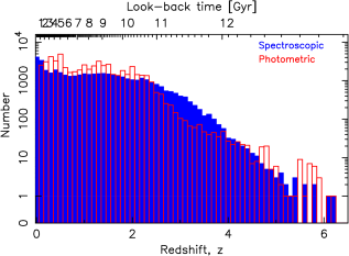
Figure 22: The spectroscopic and published photometric redshift distributions of the Milliquas radio sources. The latter are rounded to $0.1z$ (Flesch, 2021) and so there no photometric redshifts with $z_{\text{phot}}<0.1$.

Again, scraping the NIR–optical–UV photometry from NED, WISE and GALEX (Sect. 2.3.2), only 4844 of the 56 535 sources have all nine magnitudes (Table 12),

Table 12: The number of magnitude measurements in each of the bands for the 56 535 Milliquas radio associated sources with photometric redshifts.

$FUV$	$NUV$	$u$	$g$	$r$	$i$	$z$	$W1$	$W2$
12 200	31 326	22 070	24 066	24 543	29 876	33 394	54 102	54 454

with the largest deficit being in the $FUV$. Given that the $NUV$ magnitude is detected in 55% of the sources, suggests that this may be a sensitivity issue. We could impute some of the missing magnitudes to increase the sample size, but 4844 should be sufficient to compare with the Milliquas photometric redshifts without compromising our model.

Showing the redshifts we predict from our ANN (Sect. 4.2.1)

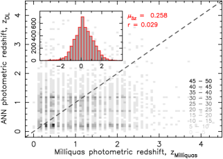
Figure 23: The ANN photometric redshifts versus those of the Milliquas (Flesch, 2021). $n=4844$, $\sigma_{\Delta z}=0.92$, $\mu_{\Delta z}=0.26$, $\sigma_{\text{MAD}}=0.90$, $\mu_{\Delta z(\text{norm})}=0.02$, $\sigma_{\Delta z(\text{norm})}=0.47$, $\sigma_{\text{NMAD}}=0.45$ and $\eta=74$%.

against those of the Milliquas using the four-colour method (Fig. 23), suggests that these are generally unreliable. The four-colour method estimates photometric redshifts from the $u-g,g-r$, $r-i$ and $i-z$ colours (Flesch, 2015), but due to the shifting of rest-frame features into other observing bands, the NIR and UV colours (or magnitudes) are crucial to obtaining accurate photometric estimates over a wide range of redshifts (Curran, 2020).

References

- Athreya & Kapahi (1998) Athreya R. M., Kapahi V. K., 1998, JA&A, 19, 63
- Becker et al. (1995) Becker R. H., White R. L., Helfand D. J., 1995, ApJ, 450, 559
- Bianchi et al. (2014) Bianchi L., Conti A., Shiao B., 2014, Advances in Space Research, 53, 900
- Bianchi et al. (2017) Bianchi L., Shiao B., Thilker D., 2017, ApJS, 230, 24
- Bovy et al. (2012) Bovy J. et al., 2012, ApJ, 749, 41
- Brescia et al. (2013) Brescia M., Cavuoti S., D’Abrusco R., Longo G., Mercurio A., 2013, ApJ, 772, 140
- Bridle et al. (1972) Bridle A. H., Kesteven M. J. L., Guindon B., 1972, Astrophysical Letters, 11, 27
- Carvajal et al. (2021) Carvajal R., Matute I., Afonso J., Amarantidis S., Barbosa D., Cunha P., Humphrey A., 2021, A New Window on the Radio Emission from Galaxies, Galaxy Clusters and Cosmic Web: Current Status and Perspectives
- Ching et al. (2017) Ching J. H. Y. et al., 2017, MNRAS, 464, 1306
- Curran et al. (2013) Curran S., Whiting M. T., Sadler E. M., Bignell C., 2013, MNRAS, 428, 2053
- Curran (2020) Curran S. J., 2020, MNRAS, 493, L70
- Curran (2021) Curran S. J., 2021, MNRAS, 508, 1165
- Curran (2022) Curran S. J., 2022, MNRAS, 512, 2099
- Curran et al. (2019) Curran S. J., Hunstead R. W., Johnston H. M., Whiting M. T., Sadler E. M., Allison J. R., Athreya R., 2019, MNRAS, 484, 1182
- Curran & Moss (2019) Curran S. J., Moss J. P., 2019, A&A, 629, A56
- Curran et al. (2021) Curran S. J., Moss J. P., Perrott Y. C., 2021, MNRAS, 503, 2639
- Curran & Whiting (2012) Curran S. J., Whiting M. T., 2012, ApJ, 759, 117
- Curran et al. (2011) Curran S. J. et al., 2011, MNRAS, 416, 2143
- de Vries et al. (1997) de Vries W. H., Barthel P. D., O’Dea C. P., 1997, A&A, 321, 105
- Fanti (2000) Fanti C., 2000, in EVN Symposium 2000, Proceedings of the 5th European VLBI Network Symposium, Conway J. E., Polatidis A. G., Booth R. S., Pihlström Y. M., eds., Onsala Space Observatory, Chalmers Technical University, Göteborg, Sweden, p. 73
- Flesch (2015) Flesch E. W., 2015, PASA, 32, 1
- Flesch (2021) Flesch E. W., 2021, arXiv e-prints, arXiv:2105.12985
- Gibson et al. (2022) Gibson S. J., Narendra A., Dainotti M. G., Bogdan M., Pollo A., Poliszczuk A., Rinaldi E., Liodakis I., 2022, Frontiers in Astronomy and Space Sciences, arXiv:2203.00087
- Han et al. (2016) Han B., Ding H.-P., Zhang Y.-X., Zhao Y.-H., 2016, Research in Astronomy and Astrophysics, 16, 74
- Li et al. (2021) Li C. et al., 2021, MNRAS, 509, 2289
- Luken et al. (2021) Luken K. J., Padhy R., Wang X. R., 2021, in Machine Learning for Physical Sciences workshop at NeurIPS 2021
- Ma et al. (2009) Ma C. et al., 2009, IERS Technical Note, 35, 1
- Maddox et al. (2012) Maddox N., Hewett P. C., Péroux C., Nestor D. B., Wisotzki L., 2012, MNRAS, 424, 2876
- Majic & Curran (2015) Majic R. A. M., Curran S. J., 2015, Radio Photometric Redshifts: Estimating radio source redshifts from their spectral energy distributions. Tech. rep., Victoria University of Wellington
- Malkin (2018) Malkin Z., 2018, ApJS, 239, 20
- Menon (1983) Menon T. K., 1983, AJ, 88, 598
- Morganti et al. (2015) Morganti R., Sadler E. M., Curran S., 2015, Advancing Astrophysics with the Square Kilometre Array (AASKA14), 134
- Nakoneczny et al. (2021) Nakoneczny S. J. et al., 2021, A&A, 649, A81
- Norris et al. (2011) Norris R. P. et al., 2011, PASA, 28, 215
- Norris et al. (2019) Norris R. P. et al., 2019, PASP, 131, 108004
- O’Dea (1998) O’Dea C. P., 1998, PASP, 110, 493
- O’Dea & Baum (1997) O’Dea C. P., Baum S. A., 1997, AJ, 113, 148
- Orienti et al. (2006) Orienti M., Morganti R., Dallacasa D., 2006, A&A, 457, 531
- Pâris et al. (2018) Pâris I. et al., 2018, A&A, 613, A51
- Richards et al. (2001) Richards G. T. et al., 2001, AJ, 122, 1151
- Skrutskie et al. (2006) Skrutskie M. F. et al., 2006, AJ, 131, 1163
- Snellen et al. (1998) Snellen I. A. G., Schilizzi R. T., de Bruyn A. G., Miley G. K., Rengelink R. B., Roettgering H. J., Bremer M. N., 1998, A&AS, 131, 435
- Turner et al. (2020) Turner R. J., Drouart G., Seymour N., Shabala S. S., 2020, MNRAS, 499, 3660
- Weinstein et al. (2004) Weinstein M. A. et al., 2004, ApJS, 155, 243
- White et al. (1997) White R. L., Becker R. H., Helfand D. J., Gregg M. D., 1997, ApJ, 475, 479
- Wolf et al. (2018) Wolf C. et al., 2018, PASA, 35, 10