Optimizing a DIscrete Loss (ODIL) to solve forward and inverse problems for partial differential equations using machine learning tools

Abstract

We introduce the Optimizing a Discrete Loss (ODIL) framework for the numerical solution of Partial Differential Equations (PDE) using machine learning tools. The framework formulates numerical methods as a minimization of discrete residuals that are solved using gradient descent and Newton’s methods. We demonstrate the value of this approach on equations that may have missing parameters or where no sufficient data is available to form a well-posed initial-value problem. The framework is presented for mesh based discretizations of PDEs and inherits their accuracy, convergence, and conservation properties. It preserves the sparsity of the solutions and is readily applicable to inverse and ill-posed problems. It is applied to PDE-constrained optimization, optical flow, system identification, and data assimilation using gradient descent algorithms including those often deployed in machine learning. We compare ODIL with related approach that represents the solution with neural networks. We compare the two methodologies and demonstrate advantages of ODIL that include significantly higher convergence rates and several orders of magnitude lower computational cost. We evaluate the method on various linear and nonlinear partial differential equations including the Navier-Stokes equations for flow reconstruction problems.

Main

Classical numerical solutions for partial differential equations (PDE) rely on their discretization, for example by finite difference [10] or finite element techniques [23], given initial and boundary conditions. However, these techniques may not be readily extended for problems where either the equations have missing parameters or no sufficient data is available to form a correct initial-value problem. Such problems are encountered in various fields of science and engineering and they are handled by various methods such as PDE-constrained optimization [6], data assimilation [11], optical flow in computer vision [4], and system identification [12]. There is a strong need to develop efficient methods for solving such equations efficiently.

One approach for solving such problems represents the solution using neural networks. This approach was introduced by Lagaris et al. [9]. At the time, the method did not offer significant advantages for solving ODEs and PDEs in particular due to its computational cost. Neural networks were also applied for back-tracking of an $N$-body system [16]. Twenty years later, the method was revived by Raissi et al. [17] who used modern machine learning methods and software (such as deep neural networks, automatic differentiation, and TensorFlow) to carry out its operations. The method has been popularized by the term physics-informed neural network (PINN).

PINNs cannot match standard numerical methods for solving classical well-posed problems involving PDEs but they were positioned as a universal and convenient tool for solving ill-posed and inverse problems. However, to the best of our knowledge, there is no baseline for comparison and assessment of the capabilities of these methods. While the authors admit that conventional numerical solvers are more efficient for classical problems [17], a direct comparison with such solvers reveals important drawbacks of the neural network approach.

In PINNs, the cost of evaluating the solution at one point is proportional to the number of weights of the neural network, while for conventional grid-based methods the cost is constant. Furthermore, as each weight of the neural network affects the solution at all points, the method is not consistent with the locality of the original differential problem. This is a crucial issue as in PINNs, even for linear problems, the solution is approximated by nonlinear neural networks. Consequently, the gradient of the residual with respect to the weights at one point is a dense vector and the Hessian of the loss function is a dense matrix. This makes efficient optimization methods such as Newton’s method unsuitable. In contrast, for linear problems Newton’s method would find the solution exactly after one step and for nonlinear problems would converge quadratically and typically require few iterations to reach the desired accuracy. The supposed convenience of representation and ease of formalism by PINN comes with a cost. While PINN evaluates the differential operator exactly on a set of collocation points, it makes no allowance for physically and numerically motivated adjustments that speed up convergence and ensure discrete conservation such as deferred correction, upwind schemes, and discrete conservation laws as represented in the finite volume method. Furthermore, decades of development and analysis that went into conventional solvers enables understanding, prediction, and control of their convergence and stability properties. Such information is not available with neural networks and recent works are actually aiming to remedy this situation [14] Nevertheless, the PINN framework is actively studied as a tool to solve ill-posed and inverse problems [7].

We introduce the Optimizing a Discrete Loss (ODIL) framework that combines discrete formulations of PDEs with modern machine learning tools to extend their scope to ill-posed and inverse problems. The idea of solving the discrete equations as a minimization problem is known as the discretize-then-differentiate approach in the context of PDE-constrained optimization [6], has been formulated for linear problems as the penalty method [19], and is related to the 4D-VAR problem in data assimilation [11]. This procedure has two key aspects. Firstly, the discretization itself, that defines the accuracy, stability and consistency of the method. Secondly, the optimization algorithm to solve the discrete problem. Our method uses efficient computational tools that are available for both of these aspects. The discretization properties are inherited from the classical numerical methods building upon the advances in this field over multiple decades. Since the sparsity of the problem is preserved, the optimization algorithm can use a Hessian and achieve a quadratic converge rate, which remains out of reach for gradient-based training of neural networks. Our use of automatic differentiation to compute the Hessian, makes the implementation as convenient as applying gradient-based methods.

Results

Wave equation. Accuracy and cost of PINN

In this section, we apply ODIL to the solution of the initial-value problem for the wave equation $u_{tt}=u_{xx}$. We compare the results of ODIL with those of PINNS in terms of accuracy and computational cost. Both methods reduce the problem to a minimization of a loss function. ODIL represents the solution on a uniform grid and constructs the loss from a second-order finite volume discretization of the equation, while PINN represents the solution as a fully connected neural network and evaluates the residuals of the original differential equation exactly on a finite set of collocation points [17]. The initial conditions for $u$ and $u_{t}$ and Dirichlet conditions on the boundaries are specified from an exact solution $u(x,t)=\tfrac{1}{10}\sum_{k=1}^{5}(\cos{(x-t+0.5)\pi k}+\cos{(x+t+0.5)\pi k})$ in a rectangular domain $x\in(-1,1),\;t\in(0,1)$. For a given number of parameters $N$, ODIL represents the solution on a $\sqrt{N}\times\sqrt{N}$ grid, while PINN consists of two equally sized hidden layers with $\tanh$ activation functions and $N$ being the total number of weights. The number of collocation points for PINN is fixed and amounts to 8192 points inside the domain and 768 points for the initial and boundary conditions. Figure 1 shows examples of the solutions obtained using both methods as well as measurements of their accuracy and cost depending on the number of parameters. The measurements for PINN include 25 samples for the random initial weights and positions of the collocation points. In the case of ODIL, solutions from two optimization methods L-BFGS-B and Newton coincide. The execution time is a product of the number of optimization epochs required to reach a 150% of the error obtained after 80000 epochs and an average execution time over the last 100 epochs. The measurements are performed on Intel Xeon E5-2690 v3 CPUs. Both methods demonstrate similar accuracy. The error of ODIL scales as $1/N$ corresponding to a second-order accurate discretization. The error of PINN is significantly scattered, although the median error also scales as $1/N$. The execution times, however, are drastically different. With $N=20000$ parameters, optimization of PINN using L-BFGS-B takes 15 hours, optimization of ODIL using L-BFGS-B takes 40 minutes, and Newton with a direct linear solver [20] takes only 0.5 seconds, which is $100\,000$ times faster than PINNs.

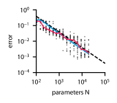
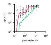
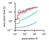
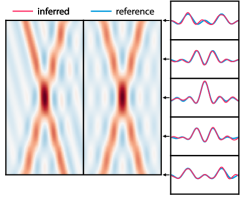
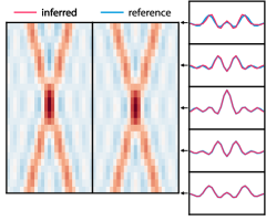
PINN

ODIL

Figure 1: Wave equation solved using PINN and ODIL. Top: $L_{2}$-error, number of epochs, and execution time of various methods: PINN optimized with L-BFGS-B  , ODIL optimized with L-BFGS-B  , ODIL optimized with Newton  , and line with slope $1/N$  . The dots correspond to samples of the initial weights and collocation points of PINN. The number of parameters is the number of weights for PINN and the number of grid points for ODIL. Bottom: Examples of solutions obtained using PINN with two hidden layers of 25 neurons and ODIL on a $25\times 25$ grid.

Lid-driven cavity. Forward problem

The lid-driven cavity problem is a standard test case [5] for numerical methods for the steady-state Navier-Stokes equations in two dimensions: $u_{x}+v_{y}=0$, $uu_{x}+vu_{y}=-p_{x}+1/\mathrm{Re}(u_{xx}+u_{yy})$, $uv_{x}+vv_{y}=-p_{y}+1/\mathrm{Re}(v_{xx}+v_{yy})$, where $u(x,y)$ and $v(x,y)$ are the two velocity components and $p(x,y)$ is the pressure. The problem is solved in a unit domain with no-slip boundary conditions. The upper boundary is moving to the right at a unit velocity while the other boundaries are stagnant. We use a finite volume discretization on a uniform Cartesian grid with $128\times 128$ cells based on the SIMPLE method [15, 3] with the Rhie-Chow interpolation [18] to prevent oscillations in the pressure field and the deferred correction approach that treats high-order discretization explicitly and low-order discretization implicitly to obtain an operator with a compact stencil.

Figure 2 shows the streamlines for values of $\mathrm{Re}$ between 100 and 3200, as well as a convergence history of various optimization algorithms. The $L_{2}$ error is computed relative to the solution of the discrete problem. The number of iterations it takes for L-BFGS-B to reach an error of $10^{-3}$ at $\mathrm{Re}=400$ is in the order of $10000$ which is comparable to the number of iterations typically needed for training PINNs for flow problems [17]. Adam has only reached an error of $0.05$ even after 50 000 iterations. Conversely, Newton’s method takes about 10 iterations to reach an error of $10^{-6}$, and the number of iterations does not significantly change between $\mathrm{Re}=100$ and $400$.

$\mathrm{Re}=100$

$\mathrm{Re}=400$

$\mathrm{Re}=1000$

$\mathrm{Re}=3200$

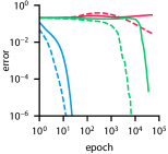
Figure 2: Lid-driven cavity problem solved with ODIL. Left: streamlines at various $\mathrm{Re}$. Right: History of the $L_{2}$-error from various optimization algorithms: Adam  , L-BFGS-B  , and Newton   at $\mathrm{Re}=100$; Adam  , L-BFGS-B  , and Newton   at $\mathrm{Re}=400$.

Lid-driven cavity. Flow reconstruction

Here we solve the same equations as in the previous case, but instead of the no-slip we only impose free-slip boundary conditions and additionally require that the velocity field equals a reference velocity field in a finite set of points. The loss function is a sum of three types of terms: residuals of equations, terms to impose known velocity values, and a regularization term $k^{2}_{\mathrm{reg}}\big{(}\|u_{xx}\|^{2}+\|u_{yy}\|^{2}+\|v_{xx}\|^{2}+\|v_{yy}\|^{2}\big{)}$ with $k_{\mathrm{reg}}=10^{-4}$. The problem is solved on a $128\times 128$ grid and the reference velocity field is obtained from the forward problem. Figure 3 shows the results of reconstruction from 32 points. Surprisingly, this small number of points is sufficient to reproduce features of the flow.

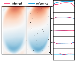
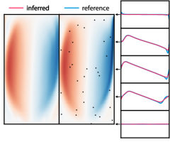
$x$-velocity

$y$-velocity

Figure 3: Reconstruction of the lid-driven cavity flow at $\mathrm{Re}=3200$ from a finite set of points. Inferred and reference fields of $x$- and $y$-components of velocity and pressure. The reference velocity is imposed in 32 points, and the Navier-Stokes equations are imposed everywhere with free-slip boundary conditions.

Measure of flow complexity

Based on the flow reconstruction from a finite set of points, we introduce a measure of flow complexity. Consider a velocity field $\bm{u}_{\mathrm{ref}}$ that satisfies the Navier-Stokes equations. First we define the quantity $E(K)=\min\limits_{|X|=K}\|\bm{u}_{\mathrm{ref}}-\bm{u}(X)\|$ as the best reconstruction error given $K$ points, where $\bm{u}(X)$ is the velocity field reconstructed from points $X$ and the minimum is taken over all sets of $K$ points. Then we define a measure of flow complexity for a given accuracy $\varepsilon>0$ as the minimal number of points required to achieve that accuracy $K_{\mathrm{min}}(\varepsilon)=\{K\;|\;E(K)<\varepsilon\}$.

To illustrate the measure, we consider four types of flow: uniform velocity, Couette flow (linear profile), Poiseuille flow (parabolic profile), and the flow in a lid-driven cavity. The reference velocity fields in the first three cases are chosen once at an arbitrary orientation and such that the maximum velocity magnitude is unity. The problem is solved on a $64\times 64$ grid, the velocity at the boundaries is extrapolated from the inside with second order. The error is defined through the $L_{1}$ norm. The loss function includes the same regularization term as in Lid-driven cavity. Flow reconstruction with $k_{\mathrm{reg}}=10^{-3}$. Figure 4 shows the values of $E(K)$ and $K_{\mathrm{min}}(0.05)$. As expected, the uniform flow takes 1 point to reconstruct while adding higher order terms to the velocity increases the number of points. Finally, 29 points are required to reach an error of $0.05$ for the lid-driven cavity flow.

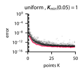
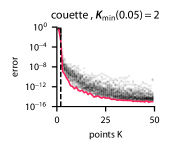
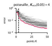
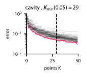
Figure 4: Fluid flow reconstruction error depending on the number of reconstruction points for various flows: uniform velocity, Couette flow, Poiseuille flow, and the flow in a lid-driven cavity. The dots correspond to samples of sets of $K$ points and the minimal value over them is an estimate of $E(K)$  .

Velocity from tracer

We consider the evolution of a tracer field governed by the advection equation in two dimensions. The problem is to find a velocity field $\bm{u}(x,y)$ given that the tracer field $c(\bm{x},t)$ satisfies the advection equation $\frac{\partial c}{\partial t}+\bm{u}\cdot\nabla{\alpha}=0$ in a unit domain, and the initial $c(\bm{x},0)=c_{0}(\bm{x})$ and final $c(\bm{x},1)=c_{1}(\bm{x})$ profiles are known. The discrete problem is solved in space and time on a $64\times 64\times 64$ grid. The loss function includes a discretization of the equation with a first-order upwind scheme, terms to impose known initial and final profiles of the tracer, and regularization terms $\|10^{-3}\nabla^{2}\bm{u}\|^{2}$ and $\|\bm{u}_{t}\|^{2}$ to prioritize velocity fields that are smooth and stationary. The results of inference are shown in Figure 5. The inferred velocity field stretches the initial tracer representing a circle to match the final profile.

Inferring the velocity field from tracers is an example of the optical flow problem [4, 13] which is important in computer vision. Furthermore, reconstructing the velocity field from a concentration field can assist experimental measurements.

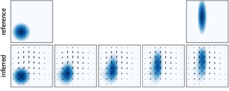
$t=0$

$0.25$

$0.5$

$0.75$

$1$

Figure 5: Inferring the velocity field from two snapshots of a tracer. The tracer satisfies the advection equation with an unknown steady velocity field. The initial and final profiles of the tracer are given. Reference tracer field (top) and inferred tracer overlaid by velocity arrows (bottom).

Discussion

We present a framework (ODIL) for computing the solutions of PDEs by casting their discretization as an optimization problem and applying optimization techniques that are widely available in machine learning software libraries. The concept of casting the PDE as a loss function has similarities with similarities with neural network formulations such as PINNs. However the fact that we use the discrete approximation of the equations allows for ODIL to be orders of magnitude more efficient in terms of computational cost and accuracy compared to the PINNs for which complex flow problems “remain elusive” [21]. The present results suggest that ODIL can be a suitable candidate for solving large scale problems such as weather prediction, complex biological flows, and other scientific and industrial simulations.

Methods

In the following, we formulate the ODIL framework for the one-dimensional wave equation $u_{tt}=u_{xx}$ discretized with finite differences. Instead of solving this equation by marching in time from known initial conditions, we rewrite the problem as a minimization of the loss function

$$L(u) =\sum\limits_{(i,n)\in\Omega_{h}}\Big{(}\frac{u^{n+1}_{i}-2u^{n}_{i}+u^{n-1}_{i}}{\Delta t^{2}}-\frac{u^{n}_{i+1}-2u^{n}_{i}+u^{n}_{i-1}}{\Delta x^{2}}\Big{)}^{2}$$

$$+\sum\limits_{(i,n)\in\Gamma_{h}}\big{(}u^{n}_{i}-g^{n}_{i}\big{)}^{2},$$

where the unknown parameter is the solution itself, a discrete field $u_{i}^{n}$ on a Cartesian grid. The loss function includes the residual of the discrete equation in grid points $\Omega_{h}$ and imposes boundary and initial conditions $u=g$ in grid points $\Gamma_{h}$. To solve this problem with a gradient-based method, such as Adam [8] or L-BFGS-B [22], we only need to compute the gradient of the loss which is also a discrete field $\partial L/\partial u$. To apply Newton’s method, we assume that the loss function is a sum of quadratic terms such as $L(u)=\|\bm{F}[u]\|_{2}^{2}+\|\bm{G}[u]\|_{2}^{2}$ with discrete operators $\bm{F}[u]$ and $\bm{G}[u]$ and linearize the operators about the current solution $u^{s}$ to obtain a quadratic loss

$$L^{s}(u^{s+1})=\big{\|}\bm{F}^{s}+(\partial\bm{F}^{s}/\partial u)(u^{s+1}-u^{s})\big{\|}_{2}^{2}+\big{\|}\bm{G}^{s}+(\partial\bm{G}^{s}/\partial u)(u^{s+1}-u^{s})\big{\|}_{2}^{2},$$

where $\bm{F}^{s}$ and $\bm{G}^{s}$ denote $\bm{F}[u^{s}]$ and $\bm{G}[u^{s}]$. A minimum of this function provides the solution $u^{s+1}$ at the next iteration and satisfies a linear system

$$\Big{(}(\partial\bm{F}^{s}/\partial u)^{T}(\partial\bm{F}^{s}/\partial u)+(\partial\bm{G}^{s}/\partial u)^{T}(\partial\bm{G}^{s}/\partial u)\Big{)}(u^{s+1}-u^{s})+(\partial\bm{F}^{s}/\partial u)^{T}\bm{F}^{s}+(\partial\bm{G}^{s}/\partial u)^{T}\bm{G}^{s}=0.$$

Cases with terms other than $\bm{F}$ and $\bm{G}$ are handled similarly. We further assume that $\bm{F}[u]$ and $\bm{G}[u]$ at each grid point depend only on the value of $u$ in the neighboring points. This makes the derivatives $\partial\bm{F}/\partial u$ and $\partial\bm{G}/\partial u$ sparse matrices. To implement this procedure, we use automatic differentiation in TensorFlow [1] and solve the linear system with either a direct [20] or multigrid sparse linear solver [2].

Code availability

The results are obtained using software available at https://github.com/cselab/odil.

References

- [1] Abadi, M., Agarwal, A., Barham, P., Brevdo, E., Chen, Z., Citro, C., Corrado, G. S., Davis, A., Dean, J., Devin, M., Ghemawat, S., Goodfellow, I., Harp, A., Irving, G., Isard, M., Jia, Y., Jozefowicz, R., Kaiser, L., Kudlur, M., Levenberg, J., Mané, D., Monga, R., Moore, S., Murray, D., Olah, C., Schuster, M., Shlens, J., Steiner, B., Sutskever, I., Talwar, K., Tucker, P., Vanhoucke, V., Vasudevan, V., Viégas, F., Vinyals, O., Warden, P., Wattenberg, M., Wicke, M., Yu, Y., and Zheng, X. TensorFlow: Large-scale machine learning on heterogeneous systems, 2015. Software available from tensorflow.org.
- [2] Bell, N., Olson, L. N., and Schroder, J. PyAMG: Algebraic multigrid solvers in python. Journal of Open Source Software 7, 72 (2022), 4142.
- [3] Ferziger, J. H., and Peric, M. Computational methods for fluid dynamics. Springer Science & Business Media, 2012.
- [4] Fleet, D., and Weiss, Y. Optical flow estimation. In Handbook of mathematical models in computer vision. Springer, 2006, pp. 237–257.
- [5] Ghia, U., Ghia, K. N., and Shin, C. High-Re solutions for incompressible flow using the Navier-Stokes equations and a multigrid method. Journal of computational physics 48, 3 (1982), 387–411.
- [6] Gunzburger, M. D. Perspectives in flow control and optimization. SIAM, 2002.
- [7] He, Q., Barajas-Solano, D., Tartakovsky, G., and Tartakovsky, A. M. Physics-informed neural networks for multiphysics data assimilation with application to subsurface transport. Advances in Water Resources 141 (2020), 103610.
- [8] Kingma, D. P., and Ba, J. Adam: A method for stochastic optimization. arXiv preprint arXiv:1412.6980 (2014).
- [9] Lagaris, I. E., Likas, A., and Fotiadis, D. I. Artificial neural networks for solving ordinary and partial differential equations. IEEE transactions on neural networks 9, 5 (1998), 987–1000.
- [10] LeVeque, R. J. Finite difference methods for ordinary and partial differential equations: steady-state and time-dependent problems. SIAM, 2007.
- [11] Lewis, J. M., Lakshmivarahan, S., and Dhall, S. Dynamic data assimilation: a least squares approach, vol. 13. Cambridge University Press, 2006.
- [12] Ljung, L. System Identification (2nd Ed.): Theory for the User. Prentice Hall PTR, USA, 1999.
- [13] Mang, A., Gholami, A., Davatzikos, C., and Biros, G. Pde-constrained optimization in medical image analysis. Optimization and Engineering 19, 3 (2018), 765–812.
- [14] Mishra, S., and Molinaro, R. Estimates on the generalization error of physics-informed neural networks for approximating a class of inverse problems for pdes. IMA Journal of Numerical Analysis 42, 2 (2022), 981–1022.
- [15] Patankar, S. V., and Spalding, D. B. A calculation procedure for heat, mass and momentum transfer in three-dimensional parabolic flows. In Numerical Prediction of Flow, Heat Transfer, Turbulence and Combustion. Elsevier, 1983, pp. 54–73.
- [16] Quito Jr, M., Monterola, C., and Saloma, C. Solving n-body problems with neural networks. Physical review letters 86, 21 (2001), 4741.
- [17] Raissi, M., Perdikaris, P., and Karniadakis, G. E. Physics-informed neural networks: A deep learning framework for solving forward and inverse problems involving nonlinear partial differential equations. Journal of Computational physics 378 (2019), 686–707.
- [18] Rhie, C. M., and Chow, W.-L. Numerical study of the turbulent flow past an airfoil with trailing edge separation. AIAA journal 21, 11 (1983), 1525–1532.
- [19] van Leeuwen, T., and Herrmann, F. J. A penalty method for pde-constrained optimization in inverse problems. Inverse Problems 32, 1 (2015), 015007.
- [20] Virtanen, P., Gommers, R., Oliphant, T. E., Haberland, M., Reddy, T., Cournapeau, D., Burovski, E., Peterson, P., Weckesser, W., Bright, J., van der Walt, S. J., Brett, M., Wilson, J., Millman, K. J., Mayorov, N., Nelson, A. R. J., Jones, E., Kern, R., Larson, E., Carey, C. J., Polat, İ., Feng, Y., Moore, E. W., VanderPlas, J., Laxalde, D., Perktold, J., Cimrman, R., Henriksen, I., Quintero, E. A., Harris, C. R., Archibald, A. M., Ribeiro, A. H., Pedregosa, F., van Mulbregt, P., and SciPy 1.0 Contributors. SciPy 1.0: Fundamental Algorithms for Scientific Computing in Python. Nature Methods 17 (2020), 261–272.
- [21] Wang, S., Sankaran, S., and Perdikaris, P. Respecting causality is all you need for training physics-informed neural networks. arXiv preprint arXiv:2203.07404 (2022).
- [22] Zhu, C., Byrd, R. H., Lu, P., and Nocedal, J. Algorithm 778: L-BFGS-B: Fortran subroutines for large-scale bound-constrained optimization. ACM Transactions on mathematical software (TOMS) 23, 4 (1997), 550–560.
- [23] Zienkiewicz, O. C., Taylor, R. L., and Zhu, J. Z. The finite element method: its basis and fundamentals. Elsevier, 2005.