Predefined-time Stabilization for Nonlinear Stochastic Systems

Abstract

In this paper, a control scheme for stochastic predefined-time stabilization is proposed, which improves the control effect compared with stochastic finite-time or fixed-time stabilization. The stochastic predefined-time stabilization allows the upper bound of the mathematical expectation of the settling-time function below an any given positive value. Some Lyapunov-type results for predefined-time stabilization of general stochastic Itô systems are presented. Moreover, a state feedback control scheme is designed for a class of stochastic nonlinear systems in strict-feedback form. Two simulation examples are supplied to show the usefulness of the proposed stochastic predefined-time stabilization.

,

1 Introduction

The study of convergence time of dynamic systems is of both practical and theoretical importance. For some engineering requirements, we need to control the convergence speed faster or slower. Different from Lyapunov stability, which is to study the system asymptotic behavior in an infinite time horizon, finite-time or fixed-time stability investigates the transient response of the system state in a finite time horizon. Finite-time control has important applications in robot manipulators [8]. Therefore, adaptive finite-time tracking control [17], fixed-time stabilization [21] and global fast finite-time stabilization of high-order nonlinear systems [25] have been extensively studied in recent years. However, in many practical applications, it is expected that the state trajectory of a controlled system can converge to the equilibrium point at any admissible time through appropriately adjusting control parameters [14, 27, 28]. A new concept called predefined-time stability was proposed in [24], which can achieve some consequents that cannot be provided by the traditional finite-time control schemes, such as the arbitrarily adjustable upper bound of the convergence time independent of the initial value. Recently, great progress has been made for predefined-time control of deterministic nonlinear systems [12, 18, 20, 23].

Due to wide applications of stochastic systems, stochastic analysis and synthesis have been popular research areas over the past few decades [3, 9, 16, 19, 29, 30, 31, 32, 33, 34, 35, 36]. Hence, it is very valuable to study the finite-time convergence behavior of stochastic systems and generalize the above mentioned works to stochastic systems. Recently, stochastic finite-time stability/stabilization [2, 6, 7, 30, 32, 33, 34] and stochastic fixed-time stability/stabilization [15, 26] have been studied extensively. Stochastic finite-time stability was first strictly analyzed in [32], which means that the stochastic settling-time function $T(x_{0})$ is finite almost surely and the system is stable in probability. Additionally, if we also have $\sup_{x_{0}\in{\mathcal{R}}^{n}}{\mathcal{E}}T(x_{0})<\infty$, then the stochastic uncontrolled system is called fixed-time stable. Stochastic fixed-time stability means that the system is not only finite-time stable but also $\sup_{x_{0}\in{\mathcal{R}}^{n}}{\mathcal{E}}T(x_{0})<T_{\max}$ for a fixed average time $T_{\max}$ with any initial state $x_{0}\in{\mathcal{R}}^{n}$. In order to obtain a fast convergence speed, we expect that the upper bound of the mathematical expectation of the settling-time function can be arbitrarily adjusted by a control input. Therefore, it is necessary to generalize the predefined-time concept of deterministic systems to stochastic systems. However, to the best of our knowledge, up to now, there seems no work on stochastic predetermined-time stabilization based on stochastic settling-time function. It should be mentioned that a recent work [16] studied stochastic nonlinear prescribed-time stabilization in mean square sense.

This paper investigates the problem of stochastic predefined-time stabilization of nonlinear stochastic Itô systems. The main contributions of this paper are highlighted as follows:

• Stochastic predefined-time stability and stabilization are introduced and a stochastic predefined-time stabilization theorem is obtained for general nonlinear stochastic Itô systems; see Theorem 2.1. Because predefined-time stability is stronger than finite-time stability and fixed-time stability, Theorem 2.1 is applicable to stochastic finite-time/fixed-time stabilization of [32, 26], which can also be viewed as extensions of [11, 12] to stochastic systems. Theorem 2.1 is a Lyapunov-type theorem similarly to the results of [32, 34]. Theorem 2.1 yields some useful corollaries that can be conveniently used in practice.

• The high-order nonlinear stochastic system is an important class of stochastic systems that can be used to describe many phenomena arising from mechanical systems. Its feedback stabilization has been investigated in [3, 26, 29, 30, 31]. Based on the results of Section 2, we also study the predefined-time stabilization of high-order nonlinear stochastic systems and give a practical controller design algorithm. Through adding the power integrator technique together with a corollary given in Section 2, a state feedback control scheme is given for a class of high-order stochastic nonlinear systems in strict-feedback form, which guarantees that the closed-loop system is stochastically predefined-time stabilizable. In addition, the proposed stochastic predefined-time stabilization control scheme improves some existing results [26, 7, 6].

The rest of this paper is organized as follows: In Section 2, we make some preliminaries by introducing some new definitions, theorems and corollaries, Lyapunov-type theorems about the stochastic predetermined-time stabilization are obtained. Section 3 presents the controller design procedure for high-order nonlinear stochastic systems. In Section 4, two simulation examples are given to show the effectiveness of our main results. Section 5 concludes this paper with some remarks.

Notation: $\mathcal{R}^{n}$ denotes the $n$-dimensional real Euclidean vector space. $\mathcal{R}_{+}:=[0,\infty)$. $D^{\prime}$ is the transpose of a matrix or vector $D$. $\mathcal{C}^{2}$ stands for the set of real-valued twice continuously differentiable functions. $sign(x):=1$ for $x>0$, $-1$ for $x<0$, $0$ for $x=0$. For any $b\geq 0$, $a\in\mathcal{R}$, the function $\lceil a\rfloor^{b}$ is defined as $\lceil a\rfloor^{b}=sign(a)|a|^{b}$. $\mathcal{E}$ means the mathematical expectation operator. $\mathcal{P}(A)$ represents the probability of event $A$. $I_{A}(x)$ is the indicator function, i.e., $I_{A}(x)=1$ for $x\in A$, otherwise, $I_{A}(x)=0$. ${\mathcal{K}}^{1}$-functions: A scalar continuous function $f$ defined from ${\mathcal{R}}_{+}$ to $[0,1)$ is said to be a ${\mathcal{K}}^{1}$-function if it is strictly increasing, $f(0)=0$, and $f(x)\to 1$ as $x\to\infty$.

2 Stochastic predefined-time stabilization

In this section, we will consider the following continuous-time stochastic system:

$$dx(t)=f(x(t),u(t))\,dt+g(x(t),u(t))\,dw(t),$$ (1)

$$x(0)=x_{0}\in\mathcal{R}^{n}\setminus\{0\},$$

where $x(t)\in\mathcal{R}^{n}$ represents the system state. $u\in\mathcal{R}^{n_{u}}$ stands for the control input. $w(t)$ is a standard one-dimensional Wiener process defined on the filtered probability space $(\Omega,\mathcal{F},\{{\mathcal{F}}_{t}\}_{t\geq 0},\mathcal{P})$. $u(t)\in\mathcal{R}^{n_{u}}$ stands for the control input. The admissible control set $\mathcal{U}$ consists of all ${\mathcal{F}}_{t}$-adaptive control processes $u(x(t))$, $u(0)=0$, which makes the closed-loop system

$$dx(t)=f(x(t),u(x(t)))\,dt+g(x(t),u(x(t)))\,dw$$

admits a unique weak solution in forward time for $x_{0}\in\mathcal{R}^{n}\setminus\{0\}$. In the considered system, we assume that $f:\mathcal{R}^{n}\times\mathcal{R}^{n_{u}}\rightarrow\mathcal{R}^{n}$ and $g:\mathcal{R}^{n}\times\mathcal{R}^{n_{u}}\rightarrow\mathcal{R}^{n}$ are continuous in $x$ and $u$ satisfying $f(0,0)=0$ and $g(0,0)=0$. The purpose of this section is to find an admissible control law $u(x)\in\mathcal{U}$ to stabilize the stochastic system (1) before a predefined time, i.e., achieve the stochastic predefined-time stabilization of system (1).

Remark 2.1.

When studying finite-time stable systems, we are interested in having a unique solution in forward time [1], which means that, for any non-zero initial condition $x_{0}$, $x(t,x_{0})$ is unique before reaching $0$. For stochastic finite-time stable systems, the concept is extended to the solution in the weak sense [34]. Based on the assumption of $f(0,0)=0$ and $g(0,0)=0$, the origin is an equilibrium point of (1). The following lemma gives an existence result of a weak solution to system (1). For the trajectory $x(t)$ after reaching the zero equilibrium point, the finite-time attractiveness (in Definition 2.1) is provided.

Lemma 2.1.

[33, 34] Suppose that there exits a nonnegative radially unbounded $\mathcal{C}^{2}$-function $V(x)$ for system (1), if $\mathcal{L}V(x)\leq 0$, then system (1) has a regular continuous solution for any initial value.

Remark 2.2.

The regular solution means that there is no finite explosion time with probability $1$.

Before introducing stochastic predefined-time stabilization, we will first review some well-known definitions on stochastic finite-time (fixed-time, predefined-time, respectively) stabilization.

Definition 2.1.

[34, 26] System (1) is said to be stochastically finite-time stabilizable or finite-time stabilizable in probability, if there exists a state feedback control $u(t)=u^{*}(x(t))\in\mathcal{U}$, such that the closed-loop system

$$dx(t)=f(x(t),u^{*}(x(t)))\,dt+g(x(t),u^{*}(x(t)))\,dw(t),$$ (2)

$$x(0)=x_{0}\in\mathcal{R}^{n}\setminus\{0\},$$

is stochastically finite-time stable, i.e.,

• Finite-time attractiveness: For any non-zero initial value $x_{0}$, there exists the first settling-time function $T(x_{0}):=\inf\{t:x(t,u^{*},x_{0})=0\}$, such that

  $$\mathcal{P}(T(x_{0})<\infty)=1,$$

  where $x(t,u^{*},x_{0})$ is the solution of (2). Moreover, $x(t+T(x_{0}),u^{*},x_{0})\equiv 0$, a.s., for any $t\geq 0$.

• Stability in probability: For any pair $(\alpha,\beta)$, $\alpha\in(0,1)$, $\beta>0$, there exists a $\delta(\alpha,\beta)>0$, such that for all $\|x_{0}\|<\delta(\alpha,\beta)$, we have

  $$\mathcal{P}(\|x(t,u^{*},x_{0})\|<\beta,\forall t>0)\geq 1-\alpha.$$

  Moreover, if there exists a positive constant $T_{max}$ such that

  $$\sup_{x_{0}\in\mathcal{R}^{n}\setminus\{0\}}\mathcal{E}T(x_{0})\leq T_{max},$$

  then system (2) is said to be stochastically fixed-time stable, and system (1) is said to be stochastically fixed-time stabilizable.

Remark 2.3.

In recent literature, new and improved definitions called predefined-time stable and stabilizable were proposed for deterministic systems based on fixed-time stability [12, 24]. This paper aims to extend these concepts and related results to stochastic system (1).

Definition 2.2.

System (1) is said to be stochastically predefined-time stabilizable if it is stochastically fixed-time stabilizable and for any $\varsigma>0$, there exists a control $u(t)=u^{*}(x(t))\in\mathcal{U}$, such that

$$\sup_{x_{0}\in\mathcal{R}^{n}\setminus\{0\}}\mathcal{E}T(x_{0})\leq\varsigma.$$

Remark 2.4.

Recently, another newly proposed definition called prescribed-time mean-square stability was introduced [16], which is different from Definition 2.2. Definition 2.2 is based on stochastic settling time function, when the system degenerates into deterministic systems, Definition 2.2 is consistent with the corresponding definition of deterministic systems.

Remark 2.5.

From Definitions 2.1 and 2.2, for the system (1) with non-zero initial value, there must be $x(t+T(x_{0}),u^{*},x_{0})\equiv 0$ with $t\geq 0$ and $T(x_{0})$ being the stochastic settling-time function. So, $0$ is an absorbing state. Moreover, when discussing predefined-time stabilization or finite-time stabilization control problems, a non-zero initial value is usually assumed [12, 33].

The following theorem is a Lyapunov-type theorem about stochastic predefined-time stabilization.

Theorem 2.1.

For any $\alpha>0$, if there exists a control input $u^{*}(x(t))\in\mathcal{U}$, driving the state of system (1) to satisfy

$$\mathcal{L}_{u=u^{*}}V(x)\leq-\frac{1}{\alpha}\beta(V(x)),\ x\in\mathcal{R}^{n}\setminus\{0\},$$ (3)

where $\beta:\mathcal{R}_{+}\mapsto\mathcal{R}_{+}$ with $\dot{\beta}(\cdot)\geq 0$, $\beta(s)>0$ for any $s>0$, and $\int^{\infty}_{0}\frac{1}{\beta(s)}\,ds\leq 1$, $V:\mathcal{R}^{n}\mapsto\mathcal{R}_{+}$ is a $\mathcal{C}^{2}$-positive definite and radially unbounded function, and $\mathcal{L}_{u=u^{*}}$ represents the infinitesimal generator of system (2). Then system (1) is stochastically predefined-time stabilizable, and $\sup_{x_{0}\in\mathcal{R}^{n}\setminus\{0\}}\mathcal{E}T(x_{0})\leq\alpha.$.

Proof. By Theorem 1 of [34], system (1) is stochastically finite-time stabilizable under the conditions of this theorem. Hence, in order to prove stochastic predefined-time stabilization of system (1), we only need to show that for any $\alpha>0$, the following holds:

$$\sup_{x_{0}\in\mathcal{R}^{n}\setminus\{0\}}\mathcal{E}T(x_{0})\leq\alpha.$$

Obviously, if $x_{0}=0$, it directly leads to $x(t,u^{*},x_{0})=0$ a.s. for any $t\geq 0$. So we only need to consider the case of non-zero initial state. From condition (3) and Lemma 2.1, it leads to that for each $x_{0}\neq 0$, there exists a regular continuous solution $x(t,u^{*},x_{0})$ to (1). Therefore, there exists a minimal positive integer $k_{0}\in\{1,2,\cdots,\}$ such that $\frac{1}{k_{0}}<\|x_{0}\|<k_{0}$. Define some sequences as follows:

$$\tau_{k}=\inf\left\{t\geq 0:\|x(t,u^{*},x_{0})\|\notin\left(\frac{1}{k},k\right)\right\},$$

$$\tau_{1k}=\inf\left\{t\geq 0:\|x(t,u^{*},x_{0})\|\in\left[0,\frac{1}{k}\right]\right\},$$

$$\tau_{2k}=\inf\left\{t\geq 0:\|x(t,u^{*},x_{0})\|\in\left[k,\infty\right)\right\}.$$

Considering Lemma 2.1 and the definition of the admissible control set $\mathcal{U}$, according to the definition of stopping time, sequences $\tau_{k}$, $\tau_{1k}$ and $\tau_{2k}$ are ${\mathcal{F}}_{\tau_{k}}$-, ${\mathcal{F}}_{\tau_{1k}}$- and ${\mathcal{F}}_{\tau_{2k}}$-measurable, respectively. So they are all stopping times. For convenience, in the sequel, we denote the solution $x(t,u^{*},x_{0})$ by $x(t)$ for short. We introduce a new Lyapunov function $P(x)=\int^{V(x)}_{0}\frac{\alpha}{\beta(s)}ds$. By Itô formula, we get

$$dP(x(t)) =\mathcal{L}_{u=u^{*}}P(x(t))\,dt$$

$$\ \ +\frac{\alpha}{\beta(V(x(t)))}\frac{\partial V^{\prime}}{\partial x}g(x(t),u^{*}(x(t)))\,dw(t),$$

where $\mathcal{L}_{u=u^{*}}P(x)$ can be computed as

$$\mathcal{L}_{u=u^{*}}P(x)=\frac{\alpha\mathcal{L}_{u=u^{*}}V(x)}{\beta(V(x))}$$

$$-\frac{1}{2}\frac{\alpha\dot{\beta}(V)}{\beta^{2}(V)}\left(g^{\prime}(x,u^{*})\frac{\partial V}{\partial x}\right)\left(\frac{\partial V^{\prime}}{\partial x}g(x,u^{*})\right).$$ (4)

Then, similar to Theorem 3.1 in [32], it follows that

$$\mathcal{E}P(x(t\wedge\tau_{k}))-P(x_{0})=\mathcal{E}\int^{t\wedge\tau_{k}}_{0}\mathcal{L}_{u=u^{*}}P(x(v))dv.$$ (5)

From (3) and (2), we have $\mathcal{L}_{u=u^{*}}P(x)\leq-1$ for any $x\neq 0$. So $\mathcal{E}P(x(t\wedge\tau_{k}))-P(x_{0})\leq-\mathcal{E}(t\wedge\tau_{k})$ and $\mathcal{E}(t\wedge\tau_{k})\leq P(x_{0})$ hold. Because $\{t\wedge\tau_{k}\}_{k\in\{k_{0},k_{0}+1,\cdots\}}$ is an increasing sequence of nonnegative random variables, by monotonic convergence theorem,

$$\lim_{k\rightarrow\infty}\mathcal{E}(t\wedge\tau_{k})=\mathcal{E}(\lim_{k\rightarrow\infty}t\wedge\tau_{k})=\mathcal{E}(t\wedge\tau_{\infty}).$$

Note that

$$\tau_{\infty}=\tau_{1,\infty}\wedge\tau_{2,\infty}.$$

Since $x(t,x_{0})$ is a regular solution, $\tau_{2,\infty}=\infty$ a.s.. So $\mathcal{E}(t\wedge\tau_{\infty})=\mathcal{E}(t\wedge\tau_{1,\infty})\leq P(x_{0})\leq\alpha$. Due to the arbitrariness of $x_{0}$ and $\tau_{1,\infty}=T(x_{0})$, it yields that

$$\sup_{x_{0}\in\mathcal{R}^{n}\setminus\{0\}}\mathcal{E}T(x_{0})\leq\alpha.$$

From (3) and $V(x)\geq 0$, $V_{t}:=V(x(t,u^{*},x_{0}))$ is a nonnegative continuous supermartingale with augmented filtration $\{{\mathcal{F}}_{t}\}_{t\geq 0}$. Through Doob’s optional-sampling theorem for continuous nonnegative supermartingales in [10],

$$\mathcal{E}(V_{T(x_{0})+t}|\mathcal{F}_{T(x_{0})})\leq V_{T(x_{0})}=0,\forall t\geq 0.$$

Taking expectation on both sides of the above inequality, we have $\mathcal{E}V_{T(x_{0})+t}\equiv 0$. Since $V$ is positive definite, it follows that $x(T(x_{0})+t,u^{*},x_{0})\equiv 0$, a.s.. The proof is completed.

Generally speaking, stochastic predefined-time stabilization is a special case of stochastic fixed-time stabilization, which is stronger than stochastic fixed-time stabilization. In order to illustrate the difference between these two concepts, a numerical example is presented below.

Example 2.1.

Consider a scalar system

$$dx=udt+xdw,\ x(0)=x_{0}.$$ (6)

By selecting the control input

$$u=u^{*}=-\frac{1}{2}x-x^{a}-x^{b}$$ (7)

with $a\in(0,1)$ and $b>1$, then the feedback system of (6) becomes

$$dx=(-\frac{1}{2}x-x^{a}-x^{b})\,dt+x\,dw,\ x(0)=x_{0}.$$ (8)

For system (8) and the Lyapunov function $V(x)=x^{2}$, it is easy to compute

$${\mathcal{L}}_{u=u^{*}}V(x)=-2x^{a+1}-2x^{b+1},$$

where ${\mathcal{L}}_{u=u^{*}}$ is the infinitesimal generator of system (8). According to Lemma 7 of [15], we have

$$\sup_{x_{0}\in\mathcal{R}}\mathcal{E}T(x_{0})\leq T_{max}:=\frac{1}{1-a}+\frac{1}{b-1}.$$

Hence, system (6) is stochastically fixed-time stabilizable.

In addition, for any $\alpha>0$, if we choose the control input as

$$u=u^{*}(x)=-\frac{\sqrt{\pi}}{2\alpha}sign(x)e^{x^{2}}-\frac{1}{2}x,$$ (9)

and $\mathcal{C}^{2}$-positive definite and radially unbounded function $V(x)=x^{2}$, then by Itô formula, we have

$$\mathcal{L}_{u=u^{*}}V(x) =2xu^{*}+x^{2}=x(-\frac{\sqrt{\pi}}{\alpha}sign(x)e^{x^{2}})$$

$$=-\frac{\sqrt{\pi}}{\alpha}|x|e^{x^{2}}=-\frac{\sqrt{\pi}}{\alpha}V(x)^{1/2}e^{V(x)}.$$

Let $\beta(s)=\sqrt{\pi}s^{1/2}e^{s}$, then $\beta(s)$ satisfies the conditions of Theorem 2.1. By Theorem 2.1, system (6) is also stochastically predefined-time stabilizable, and (9) is a stochastic predefined-time stabilizing controllor.

Remark 2.6.

Fixed-time stabilization is often difficult and sometimes impossible to adjust the controller gain such that achieving stabilization within a required predefined time. There is no guarantee that this upper bound can be adjusted arbitrarily. On this point, we can refer to the discussion in [12, 23]. From the above example, it is easier to tune the convergence time bound for stochastic predefined-time stabilization than stochastic fixed-time stabilization. Therefore, the stochastic fixed-time control discussed in [26] cannot achieve the effect of the stochastic predefined-time control discussed in this paper. Furthermore, this paper proves various Lyapunov-type theorems for stochastic predefined-time stabilization, and presents a design scheme of stochastic predefined-time controllers for higher-order nonlinear systems.

Remark 2.7.

Theorem 2.1 presents a Lyapunov-type result about stochastic predefined-time stabilization. When $\int^{t}_{0}\frac{1}{\beta(s)}ds<\infty$ with $t\geq 0$ replaces $\int^{\infty}_{0}\frac{1}{\beta(s)}ds\leq 1$ in Theorem 2.1, then system (1) is stochastically finite-time stabilizable [32]. In addition, if the condition $\int^{\infty}_{0}\frac{1}{\beta(s)}ds\leq 1$ is changed as $\int^{\infty}_{0}\frac{1}{\beta(s)}\,ds<\infty$, then system (1) is stochastically fixed-time stabilizable.

Corollary 2.1.

For any $\alpha>0$, if there exists a control input $u^{*}(x(t))\in\mathcal{U}$, driving the state of system (1) to satisfy

$$\mathcal{L}_{u=u^{*}}V(x)\leq-\frac{\tilde{\beta}(V(x))^{p}}{(1-p)\alpha\dot{\tilde{\beta}}(V(x))},x\in\mathcal{R}^{n}\setminus\{0\},$$ (10)

where $\tilde{\beta}(\cdot)$ is a function belonging to $\mathcal{K}^{1}$ with $\ddot{\tilde{\beta}}(\cdot)\leq 0$, $0\leq p<1$. $V:\mathcal{R}^{n}\mapsto\mathcal{R}_{+}$ is a  $\mathcal{C}^{2}$-positive definite and radially unbounded function. Then system (1) is stochastically predefined-time stabilizable, and for any $x_{0}\in\mathcal{R}^{n}\setminus\{0\}$, the first settling-time function satisfies $\mathcal{E}T(x_{0})\leq\alpha$.

Proof. Corollary 2.1 can be directly obtained by Theorem 2.1 via setting

$$\beta(s)=\frac{\tilde{\beta}(s)^{p}}{(1-p)\dot{\tilde{\beta}}(s)}.$$

We can also give another Lyapunov-type theorem inspired by [11].

Corollary 2.2.

For any $\alpha>0$, if there exists a control input $u^{*}(x(t))\in\mathcal{U}$, driving the state of system (1) to satisfy

$$\mathcal{L}_{u=u^{*}}W(x)\leq-\frac{1}{\alpha},\ x\in\mathcal{R}^{n}\setminus\{0\},$$ (11)

where $W:\mathcal{R}^{n}\mapsto\mathcal{R}_{+}$ is a $\mathcal{C}^{2}$-positive definite function with $0\leq W(s)<1$, $\lim_{s\rightarrow\infty}W(s)=1$. Then system (1) is stochastically predefined-time stabilizable, and for any $x_{0}\in\mathcal{R}^{n}\setminus\{0\}$, the first settling-time function satisfies $\mathcal{E}T(x_{0})\leq\alpha$.

Proof. Set $V(x)=-\ln(1-W(x))$. By (11), it is easy to obtain that

$$\mathcal{L}_{u=u^{*}}W(x)=e^{-V(x)}\mathcal{L}_{u=u^{*}}V(x)\leq-\frac{1}{\alpha}.$$ (12)

This gives

$$\mathcal{L}_{u=u^{*}}V(x)\leq-\frac{1}{\alpha}e^{V(x)}.$$

By setting $\beta(s)=e^{s}$, and using Theorem 2.1, we have the desired results immediately.

Corollary 2.3.

Assume there exist a $\mathcal{C}^{2}$-positive definite and radially unbounded function $V$, positive constants $a>0$, $0<b_{1}<1$, and $b_{2}>1$ satisfying $a-ab_{1}-1>0$. If for any $\alpha>0$, there exists a control input $u^{*}(x(t))\in\mathcal{U}$, such that

$$\mathcal{L}_{u=u^{*}}V(x)\leq -\frac{a-ab_{1}}{\alpha(a-ab_{1}-1)(b_{2}-1)}V(x)^{b_{2}}$$

$$-\frac{a}{\alpha}V(x)^{b_{1}}$$ (13)

for $x\in\mathcal{R}^{n}\setminus\{0\}$, then system (1) is stochastically predefined-time stabilizable, i.e., $\sup_{\forall x_{0}}\mathcal{E}T(x_{0})\leq\alpha$.

Proof. In Theorem 2.1, set

$$\beta(V(x))=aV(x)^{b_{1}}+\frac{a-ab_{1}}{(a-ab_{1}-1)(b_{2}-1)}V(x)^{b_{2}}.$$

Obviously, $\beta(s)\geq 0$ for $s\in{\mathcal{R}}_{+}$, and $\dot{\beta}(\cdot)\geq 0$. Moreover,

$$\int^{\infty}_{0}\frac{1}{\beta(s)}ds=\int^{1}_{0}\frac{1}{\beta(s)}ds+\int^{\infty}_{1}\frac{1}{\beta(s)}\,ds$$

$$\leq \int^{1}_{0}\frac{1}{as^{b_{1}}}\,ds+\int^{\infty}_{1}\frac{(a-ab_{1}-1)(b_{2}-1)}{(a-ab_{1})s^{b_{2}}}\,ds$$

$$= \frac{1}{(1-b_{1})a}+\frac{a-ab_{1}-1}{a-ab_{1}}=1.$$

Therefore, (2.3) implies that conditions of Theorem 2.1 are satisfied. This corollary is proved.

3 Controller design in strict-feedback form

In this section, we address the stochastic predefined-time stabilization problem for nonlinear stochastic systems based on backstepping method. Consider the following high-order stochastic nonlinear system described by

$$\begin{cases}dx_{i}=(h_{i}\lceil x_{i+1}\rfloor^{q_{i}}+f_{i}(\bar{x}_{i}))dt+g_{i}(\bar{x}_{i})dw,\\ dx_{n}=(h_{n}\lceil u\rfloor^{q_{n}}+f_{n}(x))dt+g_{n}(x)dw,\end{cases}$$ (14)

where $i=1,2,\cdots,n-1$, $x=[x_{1},\cdots,x_{n}]^{\prime}\in\mathcal{R}^{n}$ stands for the system state, $u\in\mathcal{R}$ is the control input. $w$ is a one-dimensional standard Wiener process defined on the filtered probability space $(\Omega,{\mathcal{F}}$, $\{{\mathcal{F}}_{t}\}_{t\geq 0}$, ${\mathcal{P}})$. $\bar{x}_{i}$ is defined as $\bar{x}_{i}=[x_{1},\cdots,x_{i}]^{\prime}$. $h_{1},\cdots,h_{n}$ are unknown virtual control coefficients. The drift terms $f_{i}(x)$ and diffusion terms $g_{i}(x)$, $i=1,2,\cdots,n$, are Borel measurable continuous functions with $f_{i}(0)=0$ and $g_{i}(0)=0$. For any $i$, $1<q_{i}\in\mathcal{R}_{+}$ is called the high-order of system (14).

The following assumption allows the functions $f_{i}(\bar{x}_{i})$ and $g_{i}(\bar{x}_{i})$ to have high-order and low-order nonlinear growth rates.

Assumption 3.1.

For any $i=1,2,\cdots,n$, the drift term $f_{i}(\bar{x}_{i})$ and the diffusion term $g_{i}(\bar{x}_{i})$ satisfy the following conditions:

$$|f_{i}(\bar{x}_{i})|\leq\phi_{i}(\bar{x}_{i})\sum^{i}_{j=1}|x_{j}|^{\varpi_{ij}+\frac{r_{i}+\kappa}{r_{j}}},$$

$$|g_{i}(\bar{x}_{i})|\leq\varphi_{i}(\bar{x}_{i})\sum^{i}_{j=1}|x_{j}|^{\rho_{ij}+\frac{2r_{i}+\kappa}{2r_{j}}},$$

where $\varpi_{ij}\geq 0$, $\rho_{ij}\geq 0$, $\phi_{i}(\bar{x}_{i})$ and $\varphi_{i}(\bar{x}_{i})$ are non-negative smooth functions with $\phi_{i}(0)=0$ and $\varphi_{i}(0)=0$, $\kappa\in(-\frac{1}{1+\sum^{n-1}_{s=1}q_{1}\cdots q_{s}},0)$. $r_{i+1}$ is recursively defined as $r_{i+1}=\frac{r_{i}+\kappa}{q_{i}}$ with $r_{1}=1$.

Remark 3.1.

Assumption 3.1 is a common nonlinear growth rate [6, 25]. the powers in growth condition of $f_{i}(\bar{x}_{i})$ and $g_{i}(\bar{x}_{i})$ are defined as $\varpi_{ij}+\frac{r_{i}+\kappa}{r_{j}}\in\mathcal{R}_{+}$ and $\rho_{ij}+\frac{2r_{i}+\kappa}{2r_{j}}\in\mathcal{R}_{+}$, respectively. $\varpi_{ij}+\frac{r_{i}+\kappa}{r_{j}}$ and $\rho_{ij}+\frac{2r_{i}+\kappa}{2r_{j}}$ belonging to an interval $(0,\infty)$ allow $f_{i}(\bar{x}_{i})$ and $g_{i}(\bar{x}_{i})$ to have both both high-order and low-order nonlinear growth rates. Assumption 3.1 includes the counterparts in the closely related works as special cases. For example, when $\varpi_{ij}=\rho_{ij}=0$, Assumption 3.1 degenerates to Assumption 1 in [5]. If $\phi_{i}(\bar{x}_{i})$ and $\varphi_{i}(\bar{x}_{i})$ are further specialised as constants, Assumption 3.1 becomes the low-order growth rate used in [30]. When $\varpi_{ij}=1-\frac{r_{i}+\kappa}{r_{j}}$ and $\rho_{ij}=1-\frac{2r_{i}+\kappa}{2r_{j}}$, Assumption 3.1 reduces the linear-like growth rate used in [13].

Assumption 3.2.

For any $i=1,2,\cdots,n$, there exist constants $\overline{h}_{i}>0$ and $\underline{h}_{i}>0$ such that $\underline{h}_{i}\leq h_{i}\leq\overline{h}_{i}$.

Lemma 3.1.

[29] For any $a\in\mathcal{R}$ and $b\geq 2$, we have that the function $f(a):=\lceil a\rfloor^{b}\in\mathcal{C}^{2}$, $\frac{\partial f(a)}{\partial a}=b|a|^{b-1}$ and $\frac{\partial^{2}f(a)}{\partial a^{2}}=b(b-1)\lceil a\rfloor^{b-2}$.

Lemma 3.2.

[4] Suppose $0<p<1$ and $q>1$, then for any $x,y\in\mathcal{R}$, we have

$$|\lceil x\rfloor^{pq}-\lceil y\rfloor^{pq}|\leq 2^{1-p}|\lceil x\rfloor^{q}-\lceil y\rfloor^{q}|^{p}.$$

Lemma 3.3.

[22] For any positive real numbers $p$, $q$ and any real-valued function $f(x,y)>0$, the following relationship holds:

$$|x|^{p}|y|^{q}\leq\frac{p}{p+q}f(x,y)|x|^{p+q}+\frac{q}{p+q}f^{-\frac{p}{q}}(x,y)|y|^{p+q}.$$

Lemma 3.4.

[22] For any $x,y\in\mathcal{R}$, $a\geq 1$, we have $(|x|+|y|)^{\frac{1}{a}}\leq|x|^{\frac{1}{a}}+|y|^{\frac{1}{a}}\leq 2^{\frac{a-1}{a}}(|x|+|y|)^{\frac{1}{a}}$.

Lemma 3.5.

[22] $(\sum^{j}_{i=1}a_{i})^{b}\leq\max\{j^{b-1},1\}(\sum^{j}_{i=1}a_{i}^{b})$ always holds for any positive numbers $a_{1},a_{2},\cdots,a_{j}$ and $b$.

Now, we are ready to present our main theorem of this section.

Theorem 3.1.

If the high-order stochastic nonlinear system (14) satisfies Assumptions 3.1 and 3.2, then there exists a state-feedback controller such that the closed-loop system is stochastically predefined-time stabilizable.

Proof. The proof is based on inductive arguments. Step 1: Firstly, by the power integrator technique, we choose the Lyapunov function for the first subsystem as $V_{1}(x_{1})=\int^{x_{1}}_{x_{1}^{*}}\lceil\lceil s\rfloor^{\frac{r}{r_{1}}}-\lceil x_{1}^{*}\rfloor^{\frac{r}{r_{1}}}\rfloor^{\frac{4r-\kappa-r_{1}}{r}}\,ds$, where $r\geq\max_{1\leq i\leq n}\{2r_{i}\}$ and $x^{*}_{1}=0$. By Itô’s formula, Assumption 3.1, and Lemma 3.1, we can get that

$$\mathcal{L}_{1}V_{1}(x_{1})$$

$$= \frac{\partial V_{1}}{\partial x_{1}}(h_{1}\lceil x_{2}\rfloor^{q_{1}}+f_{1}(\bar{x}_{1}))+\frac{1}{2}\frac{\partial^{2}V_{1}}{\partial x_{1}^{2}}|g_{1}(\bar{x}_{1})|^{2}$$

$$= \lceil\xi_{1}\rfloor^{\frac{4r-\kappa-r_{1}}{r}}(h_{1}\lceil x_{2}\rfloor^{q_{1}}+f_{1}(\bar{x}_{1}))+\frac{4r-\kappa-r_{1}}{2r}|\xi_{1}|^{\frac{3r-\kappa-r_{1}}{r}}$$

$$\frac{r}{r_{1}}|x_{1}|^{\frac{r}{r_{1}}-1}|g_{1}(\bar{x}_{1})|^{2}$$

$$\leq \lceil\xi_{1}\rfloor^{\frac{4r-\kappa-r_{1}}{r}}h_{1}(\lceil x_{2}\rfloor^{q_{1}}-\lceil x_{2}^{*}\rfloor^{q_{1}})+\lceil\xi_{1}\rfloor^{\frac{4r-\kappa-r_{1}}{r}}h_{1}\lceil x_{2}^{*}\rfloor^{q_{1}}$$

$$+\frac{4r-\kappa-r_{1}}{2r}|\xi_{1}|^{\frac{3r-\kappa-r_{1}}{r}}\frac{r}{r_{1}}|x_{1}|^{\frac{r}{r_{1}}-1}(\bar{\varphi}_{1}(\bar{x}_{1})|x_{1}|^{\frac{2r_{1}+\kappa}{2r_{1}}})^{2}$$

$$+\lceil\xi_{1}\rfloor^{\frac{4r-\kappa-r_{1}}{r}}\bar{\phi}_{1}(x_{1})|x_{1}|^{\frac{r_{1}+\kappa}{r_{1}}}$$

$$\leq \lceil\xi_{1}\rfloor^{\frac{4r-\kappa-r_{1}}{r}}h_{1}(\lceil x_{2}\rfloor^{q_{1}}-\lceil x_{2}^{*}\rfloor^{q_{1}})+\lceil\xi_{1}\rfloor^{\frac{4r-\kappa-r_{1}}{r}}h_{1}\lceil x_{2}^{*}\rfloor^{q_{1}}$$

$$+|\xi_{1}|^{4}\bar{\phi}_{1}(x_{1})+\frac{4r-\kappa-r_{1}}{2r_{1}}|\xi_{1}|^{4}\bar{\varphi}_{1}^{2}(\bar{x}_{1}),$$

where $\xi_{1}=\lceil x_{1}\rfloor^{\frac{r}{r_{1}}}$, $\bar{\varphi}_{1}(x_{1})\geq\varphi_{1}(x_{1})|x_{1}|^{\rho_{11}}$ and $\bar{\phi}_{1}(x_{1})\geq\phi_{1}(x_{1})|x_{1}|^{\varpi_{11}}$ are smooth functions. $\mathcal{L}_{1}$ is the infinitesimal generator of the first subsystem. The definitions of $\bar{\varphi}_{i}(\bar{x}_{i})$ and $\bar{\phi}_{i}(\bar{x}_{i})$ used in the later proof are similar and will not be repeated. Designing $x_{2}^{*}=-\beta_{1}\lceil\xi_{1}\rfloor^{\frac{r_{2}}{r}}$ and $\beta_{1}>0$, it leads to

$$\lceil x_{2}^{*}\rfloor^{q_{1}}= sign(-\beta_{1}\lceil\xi_{1}\rfloor^{\frac{r_{2}}{r}})|\beta_{1}\lceil\xi_{1}\rfloor^{\frac{r_{2}}{r}}|^{q_{1}}$$

$$= -sign(\lceil\xi_{1}\rfloor^{\frac{r_{2}}{r}})|\beta_{1}\lceil\xi_{1}\rfloor^{\frac{r_{2}}{r}}|^{q_{1}}$$

$$= -\beta_{1}^{q_{1}}\lceil\xi_{1}\rfloor^{\frac{r_{2}q_{1}}{r}}.$$

Note that $\lceil\xi_{1}\rfloor^{\frac{4r-\kappa-r_{1}}{r}}\lceil\xi_{1}\rfloor^{\frac{r_{2}q_{1}}{r}}=|\xi_{1}|^{4}$. Set $\beta_{1}(x_{1})=\left(\frac{4r-\kappa-r_{1}}{2r_{1}\overline{h}_{1}}\bar{\varphi}_{1}^{2}(x_{1})+\frac{nk_{1}}{\overline{h}_{1}k_{4}}+\frac{k_{2}}{\overline{h}_{1}k_{4}}|\xi_{1}|^{k_{3}}+\frac{\bar{\phi}_{1}(x_{1})}{\overline{h}_{1}}\right)^{\frac{1}{q_{1}}}$ with $k_{1}$, $k_{2}$, $k_{3}$, $k_{4}$ to be designed in the future. Then

$$\mathcal{L}_{1}V_{1}(x_{1})\leq \lceil\xi_{1}\rfloor^{\frac{4r-\kappa-r_{1}}{r}}h_{1}(\lceil x_{2}\rfloor^{q_{1}}-\lceil x_{2}^{*}\rfloor^{q_{1}})$$

$$-\frac{nk_{1}}{k_{4}}|\xi_{1}|^{4}-\frac{k_{2}}{k_{4}}|\xi_{1}|^{4+k_{3}}.$$

Step 2-Inductive assumption: Suppose for $j\in\{3,4,\cdots,n\}$, there is a $\mathcal{C}^{2}$- positive definite radially unbounded function $V_{j-1}$, and a set of virtual controllers $x_{1}^{*},x_{2}^{*},\cdots,x_{j}^{*}$ defined by

$$\begin{array}[]{cccc}x_{1}^{*}=0,&\xi_{1}=\lceil x_{1}\rfloor^{\frac{r}{r_{1}}}-\lceil x_{1}^{*}\rfloor^{\frac{r}{r_{1}}};\\ x_{2}^{*}=-\beta_{1}(\bar{x}_{1})\lceil\xi_{1}\rfloor^{\frac{r_{2}}{r}},&\xi_{2}=\lceil x_{2}\rfloor^{\frac{r}{r_{2}}}-\lceil x_{2}^{*}\rfloor^{\frac{r}{r_{2}}};\\ \vdots&\vdots\\ x_{j}^{*}=-\beta_{j-1}(\bar{x}_{j-1})\lceil\xi_{j-1}\rfloor^{\frac{r_{j}}{r}},&\xi_{j}=\lceil x_{j}\rfloor^{\frac{r}{r_{j}}}-\lceil x_{j}^{*}\rfloor^{\frac{r}{r_{j}}}\end{array}$$

with functions $\beta_{i}(\bar{x}_{i})>0$, $i\in\{1,2,\cdots,j-1\}$, such that

$$\mathcal{L}_{j-1}V_{j-1}(\bar{x}_{j-1})\leq \lceil\xi_{j-1}\rfloor^{\frac{4r-\kappa-r_{j-1}}{r}}h_{j-1}(\lceil x_{j}\rfloor^{q_{j-1}}-\lceil x_{j}^{*}\rfloor^{q_{j-1}})$$

$$-(n-j+2)\sum^{j-1}_{i=1}\frac{k_{1}}{k_{4}}|\xi_{i}|^{4}-\sum^{j-1}_{i=1}\frac{k_{2}}{k_{4}}|\xi_{i}|^{4+k_{3}},$$ (15)

where $\mathcal{L}_{j-1}$ is the infinitesimal generator of the first $j-1$ subsystems.

Step 3: In the following, we shall show that (3) still holds when $j-1$ is replaced by $j$ with

$$V_{j}(\bar{x}_{j})=V_{j-1}(\bar{x}_{j-1})+W_{j}(\bar{x}_{j})$$ (16)

and

$$W_{j}(\bar{x}_{j})=\int^{x_{j}}_{x_{j}^{*}}\lceil\lceil s\rfloor^{\frac{r}{r_{j}}}-\lceil x_{j}^{*}\rfloor^{\frac{r}{r_{j}}}\rfloor^{\frac{4r-\kappa-r_{j}}{r}}\,ds.$$ (17)

With the help of Proposition 6.1 in Appendix, it can be deduced from $V_{j}(\bar{x}_{j})$ that

$$\mathcal{L}_{j}V_{j}(\bar{x}_{j})$$

$$\leq \lceil\xi_{j-1}\rfloor^{\frac{4r-\kappa-r_{j-1}}{r}}h_{j-1}(\lceil x_{j}\rfloor^{q_{j-1}}-\lceil x_{j}^{*}\rfloor^{q_{j-1}})$$

$$-(n-j+2)\sum^{j-1}_{i=1}\frac{k_{1}}{k_{4}}|\xi_{i}|^{4}-\sum^{j-1}_{i=1}\frac{k_{2}}{k_{4}}|\xi_{i}|^{4+k_{3}}$$

$$+\lceil\xi_{j}\rfloor^{\frac{4r-\kappa-r_{j}}{r}}h_{j}\lceil x_{j+1}\rfloor^{q_{j}}+\lceil\xi_{j}\rfloor^{\frac{4r-\kappa-r_{j}}{r}}f_{j}(\bar{x}_{j})$$

$$+\sum^{j-1}_{i=1}\frac{\partial W_{j}}{\partial x_{i}}(h_{i}\lceil x_{i+1}\rfloor^{q_{i}}+f_{i}(\bar{x}_{i}))$$

$$+\frac{1}{2}\sum^{j}_{i,m=1}\left|\frac{\partial^{2}W_{j}}{\partial x_{i}\partial x_{m}}\right|\left|g_{i}(\bar{x}_{i})^{\prime}g_{m}(\bar{x}_{m})\right|.$$ (18)

Based on Propositions 6.2-6.5 in Appendix, we estimate some terms in (3) and obtain that

$$\mathcal{L}_{j}V_{j}(\bar{x}_{j})$$

$$\leq (\alpha_{1,j}+\alpha_{2,j}+\alpha_{3,j}+\alpha_{4,j})|\xi_{j}|^{4}-(n-j+1)\sum^{j-1}_{i=1}\frac{k_{1}}{k_{4}}|\xi_{i}|^{4}$$

$$-\sum^{j-1}_{i=1}\frac{k_{2}}{k_{4}}|\xi_{i}|^{4+k_{3}}+\lceil\xi_{j}\rfloor^{\frac{4r-\kappa-r_{j}}{r}}h_{j}\lceil x_{j+1}^{*}\rfloor^{q_{j}}$$

$$+\lceil\xi_{j}\rfloor^{\frac{4r-\kappa-r_{j}}{r}}h_{j}(\lceil x_{j+1}\rfloor^{q_{j}}-\lceil x_{j+1}^{*}\rfloor^{q_{j}}).$$

It is easy to see that the virtual controller

$$x_{j+1}^{*}=-\beta_{j}\lceil\xi_{j}\rfloor^{\frac{r_{j+1}}{r}}$$

and

$$\beta_{j}= \left(\frac{(n-j+1)k_{1}}{\overline{h}_{j}k_{4}}+\frac{\alpha_{1,j}+\alpha_{2,j}+\alpha_{3,j}+\alpha_{4,j}}{\overline{h}_{j}}\right.$$

$$\left.+\frac{k_{2}}{k_{4}\overline{h}_{j}}|\xi_{j}|^{k_{3}}\right)^{\frac{1}{q_{j}}}.$$

Then

$$\mathcal{L}_{j}V_{j}(\bar{x}_{j})$$

$$\leq -(n-j+1)\sum^{j}_{i=1}\frac{k_{1}}{k_{4}}|\xi_{i}|^{4}-\sum^{j}_{i=1}\frac{k_{2}}{k_{4}}|\xi_{i}|^{4+k_{3}}$$

$$+\lceil\xi_{j}\rfloor^{\frac{4r-\kappa-r_{j}}{r}}h_{j}(\lceil x_{j+1}\rfloor^{q_{j}}-\lceil x_{j+1}^{*}\rfloor^{q_{j}}).$$ (19)

From Steps 1-3, we have proved that (19) hold for any $j\in\{1,2,\cdots,n\}$. Hence, at the $n$th step, one concludes that

$$\mathcal{L}_{n}V_{n}(\bar{x}_{n})$$

$$\leq -\sum^{n-1}_{i=1}\frac{k_{1}}{k_{4}}|\xi_{i}|^{4}-\sum^{n-1}_{i=1}\frac{k_{2}}{k_{4}}|\xi_{i}|^{4+k_{3}}+\lceil\xi_{n}\rfloor^{\frac{4r-\kappa-r_{n}}{r}}h_{n}\lceil u\rfloor^{q_{n}}$$

$$+(\alpha_{1,n}+\alpha_{2,n}+\alpha_{3,n}+\alpha_{4,n})|\xi_{n}|^{4}$$

$$\leq -\sum^{n}_{i=1}\frac{k_{1}}{k_{4}}|\xi_{i}|^{4}-\sum^{n}_{i=1}\frac{k_{2}}{k_{4}}|\xi_{i}|^{4+k_{3}}$$

with the Lyapunov function as

$$V_{n}(\bar{x}_{n})=V_{n-1}(\bar{x}_{n-1})+W_{n}(\bar{x}_{n})$$

and

$$W_{n}(\bar{x}_{n})=\int^{x_{n}}_{x_{n}^{*}}\lceil\lceil s\rfloor^{\frac{r}{r_{j}}}-\lceil x_{n}^{*}\rfloor^{\frac{r}{r_{n}}}\rfloor^{\frac{4r-\kappa-r_{n}}{r}}\,ds.$$

Consequently, the control $u$ can be designed as

$$u = -\beta_{n}\lceil\xi_{n}\rfloor^{\frac{r_{n+1}}{r}}$$

$$= -\left(\frac{k_{1}}{\bar{h}_{n}k_{4}}+\frac{k_{2}}{k_{4}\bar{h}_{n}}|\xi_{n}|^{k_{3}}+\frac{\alpha_{1,n}+\alpha_{2,n}+\alpha_{3,n}+\alpha_{4,n}}{\bar{h}_{n}}\right)^{\frac{1}{q_{n}}}$$

$$\cdot\lceil\xi_{n}\rfloor^{\frac{r_{n+1}}{r}}.$$

Based on the proof of Proposition 6.4, we can get that

$$\int^{x_{j}}_{x_{j}^{*}}\lceil\lceil s\rfloor^{\frac{r}{r_{j}}}-\lceil x_{j}^{*}\rfloor^{\frac{r}{r_{j}}}\rfloor^{\frac{4r-\kappa-r_{j}}{r}}ds\leq 2^{1-\frac{r_{j}}{r}}|\xi_{j}|^{\frac{4r-\kappa}{r}}$$

and

$$V_{n}\leq 2\sum^{n}_{i=1}|\xi_{i}|^{\frac{4r-\kappa}{r}}.$$

Setting $k_{3}\geq-\frac{\kappa}{r}$ and using Lemma 3.5 arrive at

$$-\sum^{n}_{i=1}|\xi_{i}|^{4+k_{3}}\leq-n^{\frac{-rk_{3}-\kappa}{4r-\kappa}}(\sum^{n}_{i=1}|\xi_{i}|^{\frac{4r-\kappa}{r}})^{\frac{r(4+k_{3})}{4r-\kappa}}$$

$$\leq -n^{\frac{-rk_{3}-\kappa}{4r-\kappa}}\frac{1}{2}^{\frac{r(4+k_{3})}{4r-\kappa}}V_{n}^{\frac{r(4+k_{3})}{4r-\kappa}}$$

and

$$-\sum^{n}_{i=1}|\xi_{i}|^{4}\leq-\frac{1}{2}^{\frac{4r}{4r-\kappa}}V_{n}^{\frac{4r}{4r-\kappa}}.$$

Accordingly, one has

$$\mathcal{L}_{n}V_{n}(\bar{x}_{n})\leq -\frac{k_{1}}{k_{4}}\left(\frac{V_{n}}{2}\right)^{\frac{4r}{4r-\kappa}}-\frac{k_{2}}{k_{4}}n^{\frac{-rk_{3}-\kappa}{4r-\kappa}}\left(\frac{V_{n}}{2}\right)^{\frac{4r+rk_{3}}{4r-\kappa}}.$$

Set $k_{3}>-\frac{\kappa}{r}$, $b_{1}=\frac{4r}{4r-\kappa}$, $b_{2}=\frac{4r+rk_{3}}{4r-\kappa}$, $a=2^{-b1}k_{1}$, $k_{1}>\frac{2^{b1}}{1-b_{1}}$, $k_{2}=\frac{a-ab_{1}}{(a-ab_{1}-1)(b_{2}-1)}n^{\frac{rk_{3}+\kappa}{4r-\kappa}}2^{b_{2}}$ . The control parameter $k_{4}$ can be chosen as an arbitrary positive number. Then, considering Corollary 2.3, the origin of the closed-loop system is stochastically predefined-time stabilizable and $\sup_{x_{0}\in\mathcal{R}^{n}}\mathcal{E}T(x_{0})\leq k_{4}$.

4 Simulation Examples

In this section, we present two examples to illustrate the validity of our main results.

Example 4.1.

In this example, we consider the following one-dimensional system

$$dx=(x^{\frac{5}{3}}+u)dt+x^{2}dw.$$ (20)

For system (20), the existing design schemes [12, 26] can not solve its stochastic predefined-time stabilization. Through the design method proposed in Corollary 2.3, the controller can be constructed as

$$u=-x^{\frac{5}{3}}-\frac{1}{2}x^{3}-\frac{k_{1}}{2k_{4}}x^{\frac{1}{3}}-\frac{k_{2}}{2k_{4}}x^{k_{3}},$$

where $k_{1}>4$, $k_{2}=\frac{k_{1}}{3(\frac{k_{1}}{4}-1)\frac{k_{3}-1}{2}}$, $k_{3}>1$, and $k_{4}$ is a positive control parameter that can be adjusted arbitrarily. Then, the mathematical expectation of the first time to reach the equilibrium point must be less than $k_{4}$. Here we choose $x(0)=1$, $k_{1}=4.1$, $k_{3}=3$. In order to compare the convergence speed, $k_{4}$ is selected as a variety of different values of $4$, $2$ and $0.5$. The corresponding trajectories of the states for these groups of control experiments are all described in Figure 1.

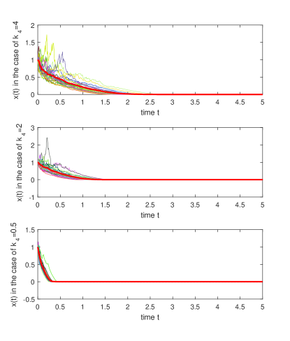
Figure 1: The state $x(t)$ of the closed-loop system (20) in the cases of $k_{4}=4,2,0.5$.

We have completed $25$ random experiments for $k_{4}=4,2,0.5$, respectively. From Figure 1, we can find that smaller $k_{4}$ leads to faster convergence speed. It is obvious that the rapidity of the convergence time meets the requirement of the stochastic fixed-time stabilization proposed in this paper.

Example 4.2.

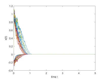
Figure 2: $x(t)$ of the closed-loop system (21) in the cases of $k_{4}=1$.

A simulation example is given to illustrate how to apply Theorem 3.1. Consider the following nonlinear stochastic system:

$$\begin{cases}dx_{1}=(h_{1}\lceil x_{2}\rfloor^{\frac{5}{3}}-\lceil x_{1}\rfloor^{\frac{3}{4}})dt+\sin(x_{1})|x_{1}|dw,\\ dx_{2}=h_{2}\lceil u\rfloor^{\frac{4}{3}}\,dt.\end{cases}$$ (21)

Clearly, Assumptions 3.1 and 3.2 are satisfied with $\underline{h}_{2}=1$, $\overline{h}_{2}=2$, $\phi_{1}=\varphi_{1}=1$, $\kappa=-\frac{1}{4}$, $\varpi_{11}=0$, $\rho_{11}=\frac{1}{8}$. According to Theorem 3.1, we can select the control parameters as $k_{1}=65.6$, $k_{2}=494.6$, $k_{3}=3.1$, $k_{4}=3$, and the control input can be designed as $u=-(10.9+3.5\beta_{1}(x_{1})+82.4|\xi_{2}|^{0.75})\lfloor\xi_{2}\rceil^{\frac{1}{8}}$ with $\beta_{1}(x_{1})=(47.1+165|\xi_{1}|^{3.1})^{0.6}$. Figure 2 shows that the designed controller renders the origin of system (21) stochastic predefined-time stabilization with $\mathcal{E}T_{f}\leq k_{4}$. This demonstrates the usability of the given design method.

5 Conclusion

In this paper, we have obtained several Lyapunov-type results about stochastic predefined-time stabilization of stochastic nonlinear systems, which extend the results of finite-time and fixed-time stabilization. Furthermore, we have presented feasible conditions and provided a constructive solution to stochastic predefined-time stabilization of a class of stochastic nonlinear systems in strict-feedback form. Two examples have been given to demonstrate the validness of the obtained results.

6 Appendix

The following proposition can be obtained from [26].

Proposition 6.1.

The following statements accordingly hold when the positive definite and proper Lyapunov function $V_{j}$ and $W_{j}$ are defined by (16) and (17) respectively.

$$\frac{\partial W_{j}}{\partial x_{j}}=\lceil\xi_{j}\rfloor^{\frac{4r-\kappa-r_{j}}{r}},$$

$$\frac{\partial W_{j}}{\partial x_{i}}=-\frac{4r-\kappa-r_{j}}{r}\int^{x_{j}}_{x_{j}^{*}}|\lceil s\rfloor^{\frac{r}{r_{j}}}-\lceil x_{j}^{*}\rfloor^{\frac{r}{r_{j}}}|^{\frac{3r-\kappa-r_{j}}{r}}ds$$

$$\ \ \cdot\frac{\partial\lceil x_{j}^{*}\rfloor^{\frac{r}{r_{j}}}}{\partial x_{i}},$$

$$\frac{\partial^{2}W_{j}}{\partial^{2}x_{j}}=\frac{4r-\kappa-r_{j}}{r_{j}}|x_{j}|^{\frac{r-r_{j}}{r_{j}}}|\xi_{j}|^{\frac{3r-\kappa-r_{j}}{r}},$$

$$\frac{\partial^{2}W_{j}}{\partial x_{i}\partial x_{j}}=\frac{\partial^{2}W_{j}}{\partial x_{j}\partial x_{i}}=-\frac{4r-\kappa-r_{j}}{r}|\xi_{j}|^{\frac{3r-\kappa-r_{j}}{r}}\frac{\partial\lceil x_{j}^{*}\rfloor^{\frac{r}{r_{j}}}}{\partial x_{i}},$$

$$\frac{\partial^{2}W_{j}}{\partial x_{i}\partial x_{m}}=\frac{(4r-\kappa-r_{j})(3r-\kappa-r_{j})}{r^{2}}\frac{\partial\lceil x_{j}^{*}\rfloor^{\frac{r}{r_{j}}}}{\partial x_{i}}\frac{\partial\lceil x_{j}^{*}\rfloor^{\frac{r}{r_{j}}}}{\partial x_{m}}$$

$$\cdot\int^{x_{j}}_{x_{j}^{*}}\lceil\lceil s\rfloor^{\frac{r}{r_{j}}}-\lceil x_{j}^{*}\rfloor^{\frac{r}{r_{j}}}\rfloor^{\frac{2r-\kappa-r_{j}}{r}}\,ds-\frac{4r-\kappa-r_{j}}{r}\frac{\partial^{2}\lceil x_{j}^{*}\rfloor^{\frac{r}{r_{j}}}}{\partial x_{i}\partial x_{m}}$$

$$\cdot\int^{x_{j}}_{x_{j}^{*}}|\lceil s\rfloor^{\frac{r}{r_{j}}}-\lceil x_{j}^{*}\rfloor^{\frac{r}{r_{j}}}|^{\frac{3r-\kappa-r_{j}}{r}}\,ds,$$

where $i,m<j$.

Next, we need to prove some necessary propositions listed below in order to estimate some terms in (3).

Proposition 6.2.

There exists a non-negative smooth function $\alpha_{1j}(\bar{x}_{j})$ such that

$$\lceil\xi_{j-1}\rfloor^{\frac{4r-\kappa-r_{j-1}}{r}}h_{j-1}(\lceil x_{j}\rfloor^{q_{j-1}}-\lceil x_{j}^{*}\rfloor^{q_{j-1}})$$

$$\leq \frac{k_{1}}{4k_{4}}|\xi_{j-1}|^{4}+\alpha_{1j}(\bar{x}_{j})|\xi_{j}|^{4}.$$

Proposition 6.3.

There exists a non-negative smooth function $\alpha_{2j}(\bar{x}_{j})$ such that

$$\lceil\xi_{j}\rfloor^{\frac{4r-\kappa-r_{j}}{r}}f_{j}(\bar{x}_{j})\leq\frac{k_{1}}{4k_{4}}\sum^{j-1}_{i=1}|\xi_{i}|^{4}+\alpha_{2j}(\bar{x}_{j})|\xi_{j}|^{4}.$$

Proposition 6.4.

There exists a non-negative smooth function $\alpha_{3j}(\bar{x}_{j})$ such that

$$\sum^{j-1}_{i=1}\frac{\partial W_{j}}{\partial x_{i}}(h_{i}\lceil x_{i+1}\rfloor^{q_{i}}+f_{i}(\bar{x}_{i}))\leq\frac{k_{1}}{4k_{4}}\sum^{j-1}_{i=1}|\xi_{i}|^{4}+\alpha_{3j}(\bar{x}_{j})|\xi_{j}|^{4}.$$

Proposition 6.5.

There exists a non-negative smooth function $\alpha_{4j}(\bar{x}_{j})$ such that

$$\frac{1}{2}\sum^{j}_{i,m=1}\left|\frac{\partial^{2}W_{j}}{\partial x_{i}\partial x_{m}}\right|\left|g_{i}(\bar{x}_{i})^{\prime}g_{m}(\bar{x}_{m})\right|\leq\frac{k_{1}}{4k_{4}}\sum^{j-1}_{i=1}|\xi_{i}|^{4}+\alpha_{4,j}|\xi_{j}|^{4}.$$

Proof of Proposition 6.2

$$\lceil\xi_{j-1}\rfloor^{\frac{4r-\kappa-r_{j-1}}{r}}h_{j-1}(\lceil x_{j}\rfloor^{q_{j-1}}-\lceil x_{j}^{*}\rfloor^{q_{j-1}})$$

$$\leq |\xi_{j-1}|^{\frac{4r-\kappa-r_{j-1}}{r}}\bar{h}_{j-1}|(\lceil x_{j}\rfloor^{q_{j-1}\frac{r}{r_{j}}})^{\frac{r_{j}}{r}}-(\lceil x_{j}^{*}\rfloor^{q_{j-1}\frac{r}{r_{j}}})^{\frac{r_{j}}{r}}|.$$

Based on Lemmas 3.2 and 3.3, and $q_{j-1}r_{j}=r_{j-1}+\kappa$, the above inequality leads to

$$\lceil\xi_{j-1}\rfloor^{\frac{4r-\kappa-r_{j-1}}{r}}\bar{h}_{j-1}(\lceil x_{j}\rfloor^{q_{j-1}}-\lceil x_{j}^{*}\rfloor^{q_{j-1}})$$

$$\leq |\xi_{j-1}|^{\frac{4r-\kappa-r_{j-1}}{r}}\bar{h}_{j-1}2^{1-\frac{r_{j-1}+\kappa}{r}}|\lceil x_{j}\rfloor^{\frac{r}{r_{j}}}-\lceil x_{j}^{*}\rfloor^{\frac{r}{r_{j}}}|^{\frac{r_{j-1}+\kappa}{r}}$$

$$\leq \frac{k_{1}}{4k_{4}}|\xi_{j-1}|^{4}+\bar{h}_{j-1}2^{1-\frac{r_{j-1}+\kappa}{r}}\frac{r_{j-1}+\kappa}{4r}\Phi_{j}^{-\frac{4r-\kappa-r_{j-1}}{r_{j-1}+\kappa}}|\xi_{j}|^{4},$$

where the real-valued function $\Phi_{j}$ can be selected as $\Phi_{j}=\frac{rk_{1}}{k_{4}(4r-\kappa-r_{j-1})\bar{h}_{j-1}2^{1-\frac{r_{j-1}+\kappa}{r}}}$. The proof is completed.

Proof of Proposition 6.3 In view of Assumption 3.1, we have

$$\lceil\xi_{j}\rfloor^{\frac{4r-\kappa-r_{j}}{r}}f_{j}(\bar{x}_{j})$$

$$\leq |\xi_{j}|^{\frac{4r-\kappa-r_{j}}{r}}\bar{\phi}_{j}(\bar{x}_{j})\sum^{j}_{i=1}||\xi_{i}|+|\beta_{i-1}|^{\frac{r}{r_{i}}}|\xi_{i-1}||^{\frac{r_{j}+\kappa}{r}}$$

with $\xi_{i}=0$. Note that $r_{j}+\kappa<r$. It is obtained from Lemma 3.4 that

$$\lceil\xi_{j}\rfloor^{\frac{4r-\kappa-r_{j}}{r}}f_{j}(\bar{x}_{j})$$

$$\leq |\xi_{j}|^{\frac{4r-\kappa-r_{j}}{r}}\bar{\phi}_{j}(\bar{x}_{j})\left(\sum^{j-1}_{i=1}(1+|\beta_{i}|^{\frac{r_{j}+\kappa}{r_{i+1}}})|\xi_{i}|^{\frac{r_{j}+\kappa}{r}}+|\xi_{j}|^{\frac{r_{j}+\kappa}{r}}\right).$$

From Lemma 3.3,

$$\lceil\xi_{j}\rfloor^{\frac{4r-\kappa-r_{j}}{r}}f_{j}(\bar{x}_{j})\leq\frac{k_{1}}{4k_{4}}\sum^{j-1}_{i=1}|\xi_{i}|^{4}+\alpha_{2j}(\bar{x}_{j})|\xi_{j}|^{4}$$

where $\alpha_{2j}$ is a non-negative smooth function. The proof is completed.

Proof of Proposition 6.4

According to Lemma 3.4 and the proof of Proposition 6.3, we have $f_{i}(\bar{x}_{i})\leq\bar{\phi}_{i}(\bar{x}_{i})\left(\sum^{i-1}_{m=1}(1+|\beta_{m}|^{\frac{r_{i}+\kappa}{r_{m+1}}})|\xi_{m}|^{\frac{r_{i}+\kappa}{r}}+|\xi_{i}|^{\frac{r_{i}+\kappa}{r}}\right)$, and $\lceil x_{i+1}\rfloor^{q_{i}}\leq|\xi_{i+1}|^{\frac{r_{i}+\kappa}{r}}+|\beta_{i}|^{\frac{r_{i}+\kappa}{r_{i+1}}}|\xi_{i}|^{\frac{r_{i}+\kappa}{r}}.$ Considering Proposition 6.1, we can get that

$$\sum^{j-1}_{i=1}\frac{\partial W_{j}}{\partial x_{i}}(h_{i}\lceil x_{i+1}\rfloor^{q_{i}}+f_{i}(\bar{x}_{i}))$$

$$\leq \sum^{j-1}_{i=1}\left|\frac{4r-\kappa-r_{j}}{r}\frac{\partial\lceil x_{j}^{*}\rfloor^{\frac{r}{r_{j}}}}{\partial x_{i}}\int^{x_{j}}_{x_{j}^{*}}|\lceil s\rfloor^{\frac{r}{r_{j}}}-\lceil x_{j}^{*}\rfloor^{\frac{r}{r_{j}}}|^{\frac{3r-\kappa-r_{j}}{r}}ds\right|$$

$$\Bigg{[}\bar{\phi}_{i}(\bar{x}_{i})\left(\sum^{i-1}_{m=1}(1+|\beta_{m}|^{\frac{r_{i}+\kappa}{r_{m+1}}})|\xi_{m}|^{\frac{r_{i}+\kappa}{r}}+|\xi_{i}|^{\frac{r_{i}+\kappa}{r}}\right)$$

$$+|\xi_{i+1}|^{\frac{r_{i}+\kappa}{r}}+|\beta_{i}|^{\frac{r_{i}+\kappa}{r_{i+1}}}|\xi_{i}|^{\frac{r_{i}+\kappa}{r}}\Bigg{]}.$$ (22)

Using Lemma 3.2, one has

$$\int^{x_{j}}_{x_{j}^{*}}\lceil\lceil s\rfloor^{\frac{r}{r_{j}}}-\lceil x_{j}^{*}\rfloor^{\frac{r}{r_{j}}}\rfloor^{\frac{3r-\kappa-r_{j}}{r}}ds\leq 2^{1-\frac{r_{j}}{r}}|\xi_{j}|^{\frac{3r-\kappa}{r}}.$$ (23)

Next, by induction, we can estimate

$$\left|\frac{\partial\lceil x_{j}^{*}\rfloor^{\frac{r}{r_{j}}}}{\partial x_{i}}\right|\leq\Theta_{1ji}\sum^{j-1}_{l=1}|\xi_{l}|^{\frac{r-r_{i}}{r}},\ j>i\geq 1,$$ (24)

where $\Theta_{1ji}$ is a non-negative smooth function. According to (6), (23) and (24), we have

$$\sum^{j-1}_{i=1}\frac{\partial W_{j}}{\partial x_{i}}(h_{i}\lceil x_{i+1}\rfloor^{q_{i}}+f_{i}(\bar{x}_{i}))$$

$$\leq \sum^{j-1}_{i=1}\frac{4r-\kappa-r_{j}}{r}2^{1-\frac{r_{j}}{r}}|\xi_{j}|^{\frac{3r-\kappa}{r}}\Theta_{1ji}\sum^{j-1}_{l=1}|\xi_{l}|^{\frac{r-r_{i}}{r}}\Theta_{2i}$$

$$\sum^{j}_{m=1}|\xi_{m}|^{\frac{r_{i}+\kappa}{r}}$$

$$\leq \frac{k_{1}}{4k_{4}}\sum^{j-1}_{i=1}|\xi_{i}|^{4}+\alpha_{3j}(\bar{x}_{j})|\xi_{j}|^{4}.$$

where $\alpha_{3j}$ is a non-negative smooth function. Proposition 6.4 is proved.

Proof of Proposition 6.5

$$\frac{1}{2}\sum^{j}_{i,m=1}\left|\frac{\partial^{2}W_{j}}{\partial x_{i}\partial x_{m}}\right|\left|g_{i}(\bar{x}_{i})^{\prime}g_{m}(\bar{x}_{m})\right|$$

$$= \frac{1}{2}\left|\frac{\partial^{2}W_{j}}{\partial^{2}x_{j}}\right|\left|g_{j}(\bar{x}_{j})^{\prime}g_{j}(\bar{x}_{j})\right|+\sum^{j-1}_{i=1}\left|\frac{\partial^{2}W_{j}}{\partial x_{j}\partial x_{i}}\right|\left|g_{j}(\bar{x}_{j})^{\prime}g_{i}(\bar{x}_{i})\right|$$

$$+\frac{1}{2}\sum^{j-1}_{i,m=1}\left|\frac{\partial^{2}W_{j}}{\partial x_{i}\partial x_{m}}\right|\left|g_{i}(\bar{x}_{i})^{\prime}g_{m}(\bar{x}_{m})\right|.$$

Firstly, based on Propositions 6.1, 6.3 and Lemma 3.5, we have

$$\frac{1}{2}\left|\frac{\partial^{2}W_{j}}{\partial^{2}x_{j}}\right|\left|g_{j}(\bar{x}_{j})^{\prime}g_{j}(\bar{x}_{j})\right|$$

$$\leq \frac{(4r-\kappa-r_{j})j}{2r_{j}}\Bigg{(}|\xi_{j}|^{\frac{r-r_{j}}{r}}+|\beta_{j-1}|^{\frac{r-r_{j}}{r_{j}}}|\xi_{j-1}|^{\frac{r-r_{j}}{r}}\Bigg{)}\bar{\varphi}_{j}(\bar{x}_{j})^{2}$$

$$|\xi_{j}|^{\frac{3r-\kappa-r_{j}}{r}}\Bigg{(}\sum^{j-1}_{s=1}(1+|\beta_{s}|^{\frac{2r_{j}+\kappa}{r_{s+1}}})|\xi_{s}|^{\frac{2r_{j}+\kappa}{r}}+|\xi_{j}|^{\frac{2r_{j}+\kappa}{r}}\Bigg{)}$$

$$\leq \Xi_{1j}(\zeta_{1j},\bar{x}_{j})|\xi_{j}|^{4}+\zeta_{1j}\sum^{j-1}_{s=1}|\xi_{s}|^{4},$$ (25)

where $\Xi_{1j}(\zeta_{1j},\bar{x}_{j})$ is a positive real function and $\zeta_{1j}$ can be an any positive real number. Next, we will consider

$$\sum^{j-1}_{i=1}\left|\frac{\partial^{2}W_{j}}{\partial x_{j}\partial x_{i}}\right|\left|g_{j}(\bar{x}_{j})^{\prime}g_{i}(\bar{x}_{i})\right|$$

$$\leq \sum^{j}_{i=1}\frac{4r-\kappa-r_{j}}{r}|\xi_{j}|^{\frac{3r-\kappa-r_{j}}{r}}\Theta_{1ji}\sum^{j-1}_{l=1}|\xi_{l}|^{\frac{r-r_{i}}{r}}\left|g_{j}(\bar{x}_{j})^{\prime}g_{i}(\bar{x}_{i})\right|.$$

Note that

$$\left|g_{j}(\bar{x}_{j})^{\prime}g_{i}(\bar{x}_{i})\right|\leq\bar{\varphi}_{i}(\bar{x}_{i})\bar{\varphi}_{j}(\bar{x}_{j})\Theta_{2ji}\sum^{j}_{s=1}|\xi_{s}|^{\frac{r_{j}+r_{i}+\kappa}{r}}$$

with $\Theta_{2ji}$ being a positive continuous function. Summarizing the above analysis leads to that

$$\sum^{j-1}_{i=1}\left|\frac{\partial^{2}W_{j}}{\partial x_{j}\partial x_{i}}\right|\left|g_{j}(\bar{x}_{j})^{\prime}g_{i}(\bar{x}_{i})\right|$$

$$\leq \sum^{j}_{i=1}\frac{(4r-\kappa-r_{j})j}{r}|\xi_{j}|^{\frac{3r-\kappa-r_{j}}{r}}\Theta_{1ji}\Theta_{2ji}\bar{\varphi}_{i}(\bar{x}_{i})\bar{\varphi}_{j}(\bar{x}_{j})$$

$$\sum^{j-1}_{l=1}|\xi_{l}|^{\frac{r-r_{i}}{r}}\sum^{j}_{s=1}|\xi_{s}|^{\frac{r_{j}+r_{i}+\kappa}{r}}$$

$$\leq \Xi_{2j}(\zeta_{2j},\bar{x}_{j})|\xi_{j}|^{4}+\zeta_{2j}\sum^{j-1}_{l=1}|\xi_{l}|^{4},$$ (26)

where $\Xi_{2j}(\zeta_{2j},\bar{x}_{j})$ is a positive real function and $\zeta_{2j}$ can be an any positive real number.

Finally, we have the following estimation:

$$\frac{1}{2}\sum^{j-1}_{i,m=1}\left|\frac{\partial^{2}W_{j}}{\partial x_{i}\partial x_{m}}\right|\left|g_{i}(\bar{x}_{i})^{\prime}g_{m}(\bar{x}_{m})\right|$$

$$\leq \sum^{j-1}_{i,m=1}\Bigg{|}\frac{(4r-\kappa-r_{j})(3r-\kappa-r_{j})}{r^{2}}\frac{\partial\lceil x_{j}^{*}\rfloor^{\frac{r}{r_{j}}}}{\partial x_{i}}\frac{\partial\lceil x_{j}^{*}\rfloor^{\frac{r}{r_{j}}}}{\partial x_{m}}$$

$$\int^{x_{j}}_{x_{j}^{*}}\lceil\lceil s\rfloor^{\frac{r}{r_{j}}}-\lceil x_{j}^{*}\rfloor^{\frac{r}{r_{j}}}\rfloor^{\frac{2r-\kappa-r_{j}}{r}}ds-\frac{4r-\kappa-r_{j}}{r}\frac{\partial^{2}\lceil x_{j}^{*}\rfloor^{\frac{r}{r_{j}}}}{\partial x_{i}\partial x_{m}}$$

$$\int^{x_{j}}_{x_{j}^{*}}|\lceil s\rfloor^{\frac{r}{r_{j}}}-\lceil x_{j}^{*}\rfloor^{\frac{r}{r_{j}}}|^{\frac{3r-\kappa-r_{j}}{r}}ds\Bigg{|}\bar{\varphi}_{i}(\bar{x}_{i})\bar{\varphi}_{m}(\bar{x}_{m})$$

$$\Theta_{2im}\sum^{j-1}_{s=1}|\xi_{s}|^{\frac{r_{m}+r_{i}+\kappa}{r}}.$$

According to (23) and (24), we have $\int^{x_{j}}_{x_{j}^{*}}\lceil\lceil s\rfloor^{\frac{r}{r_{j}}}-\lceil x_{j}^{*}\rfloor^{\frac{r}{r_{j}}}\rfloor^{\frac{2r-\kappa-r_{j}}{r}}ds\leq 2^{1-\frac{r_{j}}{r}}|\xi_{j}|^{\frac{2r-\kappa}{r}}$ and $\left|\frac{\partial\lceil x_{j}^{*}\rfloor^{\frac{r}{r_{j}}}}{\partial x_{i}}\right|\left|\frac{\partial\lceil x_{j}^{*}\rfloor^{\frac{r}{r_{j}}}}{\partial x_{m}}\right|\leq\Theta_{3jim}\sum^{j-1}_{l=1}|\xi_{l}|^{\frac{2r-r_{i}-r_{m}}{r}}$ with $\Theta_{3jim}$ being a positive real function. Therefore, we can get that

$$\sum^{j-1}_{i,m=1}\frac{(4r-\kappa-r_{j})(3r-\kappa-r_{j})}{r^{2}}\frac{\partial\lceil x_{j}^{*}\rfloor^{\frac{r}{r_{j}}}}{\partial x_{i}}\frac{\partial\lceil x_{j}^{*}\rfloor^{\frac{r}{r_{j}}}}{\partial x_{m}}$$

$$\int^{x_{j}}_{x_{j}^{*}}\lceil\lceil s\rfloor^{\frac{r}{r_{j}}}-\lceil x_{j}^{*}\rfloor^{\frac{r}{r_{j}}}\rfloor^{\frac{2r-\kappa-r_{j}}{r}}ds\bar{\varphi}_{i}(\bar{x}_{i})\bar{\varphi}_{m}(\bar{x}_{m})$$

$$\Theta_{2im}\sum^{j-1}_{s=1}|\xi_{s}|^{\frac{r_{m}+r_{i}+\kappa}{r}}$$

$$\leq \Xi_{3j}(\zeta_{3j},\bar{x}_{j})|\xi_{j}|^{4}+\zeta_{3j}\sum^{j-1}_{l=1}|\xi_{l}|^{4},$$ (27)

where $\Xi_{3j}(\zeta_{3j},\bar{x}_{j})$ is a positive real function and $\zeta_{3j}$ can be an any positive real number. Now, we are in a position to consider $\sum^{j-1}_{i,m=1}\Bigg{|}\frac{4r-\kappa-r_{j}}{r}\frac{\partial^{2}\lceil x_{j}^{*}\rfloor^{\frac{r}{r_{j}}}}{\partial x_{i}\partial x_{m}}\int^{x_{j}}_{x_{j}^{*}}|\lceil s\rfloor^{\frac{r}{r_{j}}}-\lceil x_{j}^{*}\rfloor^{\frac{r}{r_{j}}}|^{\frac{3r-\kappa-r_{j}}{r}}ds\Bigg{|}\bar{\varphi}_{i}(\bar{x}_{i})\bar{\varphi}_{m}(\bar{x}_{m})\Theta_{3im}\sum^{j-1}_{s=1}|\xi_{s}|^{\frac{r_{m}+r_{i}+\kappa}{r}}$. Through calculation, we can obtain $\frac{\partial^{2}\lceil x_{j}^{*}\rfloor^{\frac{r}{r_{j}}}}{\partial x_{i}\partial x_{m}}\leq\sum^{j-1}_{s=1}\Theta_{4jims}|\xi_{s}|^{\frac{r-r_{i}-r_{m}}{r}}$ with $\Theta_{4jims}=\prod^{j-1}_{l=s+1}|\beta_{l}^{\frac{r}{r_{l+1}}}|\Bigg{|}\frac{\partial^{2}\beta_{s}^{\frac{r}{r_{s+1}}}}{\partial x_{i}\partial x_{m}}\Bigg{|}|\xi_{s}|^{\frac{r_{i}+r_{m}}{r}}+I_{i=m}\prod^{j-1}_{l=s}|\beta_{l}^{\frac{r}{r_{l+1}}}|.$ As a consequence,

$$\sum^{j-1}_{i,m=1}\Bigg{|}\frac{4r-\kappa-r_{j}}{r}\frac{\partial^{2}\lceil x_{j}^{*}\rfloor^{\frac{r}{r_{j}}}}{\partial x_{i}\partial x_{m}}\int^{x_{j}}_{x_{j}^{*}}\lceil\lceil s\rfloor^{\frac{r}{r_{j}}}-\lceil x_{j}^{*}\rfloor^{\frac{r}{r_{j}}}\rfloor^{\frac{3r-\kappa-r_{j}}{r}}ds\Bigg{|}$$

$$\bar{\varphi}_{i}(\bar{x}_{i})\bar{\varphi}_{m}(\bar{x}_{m})\sum^{m}_{s=1}|x_{s}|^{\frac{2r_{m}+\kappa}{2r_{s}}}\sum^{i}_{s=1}|x_{s}|^{\frac{2r_{i}+\kappa}{2r_{s}}}$$

$$\leq\sum^{j-1}_{i,m=1}\frac{4r-\kappa-r_{j}}{r}2^{1-\frac{r_{j}}{r}}|\xi_{j}|^{\frac{3r-\kappa}{r}}\bar{\varphi}_{i}(\bar{x}_{i})\bar{\varphi}_{m}(\bar{x}_{m})\sum^{j-1}_{s=1}\Theta_{4jims}$$

$$|\xi_{s}|^{\frac{r-r_{i}-r_{m}}{r}}\Theta_{3im}\sum^{j-1}_{s=1}|\xi_{s}|^{\frac{r_{m}+r_{i}+\kappa}{r}}$$

$$\leq\Xi_{4j}(\zeta_{4j},\bar{x}_{j})|\xi_{j}|^{4}+\zeta_{4j}\sum^{j-1}_{s=1}|\xi_{s}|^{4}.$$ (28)

where $\Xi_{4j}(\zeta_{4j},\bar{x}_{j})$ is a positive real function and $\zeta_{4j}$ can be an any positive real number. Based on (6), (6), (6) and (6), we can find a suitable $\zeta_{ij}$ such that $\sum^{4}_{i=1}\zeta_{ij}=\frac{k_{1}}{4k_{4}}$, which completes the proof of Proposition 6.5.

References

• [1] Bhat, S. P., & Bernstein, D. S. (2000). Finite-time stability of continuous autonomous systems. SIAM Journal on Control and optimization, 38(3): 751-766.
• [2] Chen, W., & Jiao, L. C. (2010). Finite-time stability theorem of stochastic nonlinear systems. Automatica, 46(12): 2105-2108.
• [3] Cui, R. H., & Xie, X. J. (2021). Adaptive state-feedback stabilization of state-constrained stochastic high-order nonlinear systems. Science China Information Sciences, 64(10):200203:1-200203:11.
• [4] Ding, S., Li, S., & Zheng, W. (2012). Nonsmooth stabilization of a class of nonlinear cascaded systems. Automatica , 48: 2597-2606.
• [5] Fang, L., Ma, L., Ding, S., & Zhao, D. (2019). Robust finite-time stabilization of a class of high-order stochastic nonlinear systems subject to output constraint and disturbances. International Journal of Robust and Nonlinear Control, 29(16): 5550-5573.
• [6] Gao, F., Wu, Y., & Liu, Y. (2019). Finite-time stabilisation of a class of stochastic nonlinear systems with dead-zone input. International Journal of Control, 92(7): 1541-1550.
• [7] Huang, S., & Xiang, Z. (2016). Finite-time stabilization of a class of switched stochastic nonlinear systems under arbitrary switching. International Journal of Robust and Nonlinear Control, 26(10): 2136-2152.
• [8] Hong, Y., Xu, Y., Huang, J. (2002). Finite-time control for robot manipulators. Systems and Control letters, 46(4): 243-253.
• [9] Has’minskii, R. Z. (1980). Stochastic Stability of Differential Equations. Alphen: Sijtjoff and Noordhoff.
• [10] Rogers, L. C. G., & Williams, D. (2000). Diffusions, Markov processes and martingales: volume 1, foundations. Cambridge university press.
• [11] Jiménez-Rodríguez, E., Muñoz-Vázquez, A. J., Sánchez-Torres, J. D., & Loukianov, A. G. (2018). A note on predefined-time stability. IFAC-PapersOnLine, 51(13): 520-525.
• [12] Jiménez-Rodríguez, E., Muñoz-Vázquez, A. J., Sánchez-Torres, J. D., Defoort, M., & Loukianov, A. G. (2020). A Lyapunov-like characterization of predefined-time stability. IEEE Transactions on Automatic Control, 65(11): 4922-4927.
• [13] Khoo, S., Yin, J., Man, Z., & Yu, X. (2013). Finite-time stabilization of stochastic nonlinear systems in strict-feedback form. Automatica, 2013, 49(5): 1403-1410.
• [14] Krishnamurthy, P., Khorrami, F., & Krstic, M. (2020). Robust adaptive prescribed-time stabilization via output feedback for uncertain nonlinear strict-feedback-like systems. European Journal of Control, 55: 14-23.
• [15] Liang, Y., Li, Y. X., & Hou, Z. (2021). Adaptive fixed-time tracking control for stochastic pure-feedback nonlinear systems. International Journal of Adaptive Control and Signal Processing, 35(9): 1712-1731.
• [16] Li, W., & Krstic, M. (2021). Stochastic nonlinear prescribed-time stabilization and inverse optimality, IEEE Transactions on Automatic Control, doi: 10.1109/TAC.2021.3061646.
• [17] Li. H., Zhao. S., He. W., & Lu, R. (2019). Adaptive finite-time tracking control of full state constrained nonlinear systems with dead-zone. Automatica, 100: 99-107.
• [18] Muñoz-Vázquez, A. J., Fernández-Anaya G, Sánchez-Torres, J. D., & Meléndez-Vázquez, F. (2021). Predefined-time control of distributed-order systems. Nonlinear Dynamics, 103(3): 2689-2700.
• [19] Mao. X. (2007). Stochastic differential equations and applications. 2nd Edition, Horwood.
• [20] Ni, J., Liu, L., Tang, Y., & Liu, C. (2021). Predefined-time consensus tracking of second-order multiagent systems. IEEE Transactions on Systems, Man, and Cybernetics: Systems, 51(4): 2550-2560.
• [21] Polyakov, A. (2011). Nonlinear feedback design for fixed-time stabilization of linear control systems. IEEE Transactions on Automatic Control, 57(8): 2106-2110.
• [22] Qian, C., & Lin, W. (2001). A continuous feedback approach to global strong stabilization of nonlinear systems. IEEE Transactions on Automatic Control, 46: 1061-1079.
• [23] Sánchez-Torres, J. D., Muñoz-Vázquez, A. J., Defoort, M., Jiménez-Rodríguez, E., & Loukianov, A. G. (2020). A class of predefined-time controllers for uncertain second-order systems. European Journal of Control, 53: 52-58.
• [24] Sánchez-Torres, J. D., Sanchez, E. N., & Loukianov, A. G. (2015). Predefined-time stability of dynamical systems with sliding modes. 2015 American Control Conference, July 1-3, 2015, 5842-5846.
• [25] Sun, Z. Y., Yun, M. M., & Li, T. (2017). A new approach to fast global finite-time stabilization of high-order nonlinear system. Automatica, 81: 455-463.
• [26] Song, Z., Li. P., Zhai, J., Wang. Z., Huang. X. (2020). Global fixed-time stabilization for switched stochastic nonlinear systems under rational switching powers. Applied Mathematics and Computation, 387: 124856.
• [27] Song. Y., Wang. Y., Holloway. J., & Krstic, M. (2017). Time-varying feedback for regulation of normal-form nonlinear systems in prescribed finite time. Automatica, 83: 243-251.
• [28] Wang, Y., Song, Y., Hill, D. J., & Krstic, M., (2019). Prescribed-time consensus and containment control of networked multiagent systems. IEEE Transactions on Cybernetics, 49(4): 1138-1147.
• [29] Xie, X. J., Duan. N., & Zhao, C. R. (2014). A combined homogeneous domination and sign function approach to output-feedback stabilization of stochastic high-order nonlinear systems, IEEE Transactions on Automatic Control 59(5): 1303-1309.
• [30] Xie, X. J., $\&$ Li, G. J. (2019). Finite-time output-feedback stabilization of high-order nonholonomic systems. International Journal of Robust and Nonlinear Control, 29(9): 2695-2711.
• [31] Xie, X. J., & Liu, L. (2013). A Homogeneous domination approach to state feedback of stochastic high-order nonlinear systems with time-varying delay. IEEE Transactions on Automatic Control, 58(2): 494-499.
• [32] Yin, J., Khoo, S., Man, Z., & Yu, X. (2011). Finite-time stability and instability of stochastic nonlinear systems. Automatica, 47: 1288-1292.
• [33] Yin. J., & Khoo, S. (2015). Continuous finite-time state feedback stabilizers for some nonlinear stochastic systems, International Journal of Robust and Nonlinear Control, 25(11): 1581-1600.
• [34] Yu. X., Yin, J., $\&$ Khoo, S. (2019). Generalized Lyapunov criteria on finite-time stability of stochastic nonlinear systems. Automatica, 107: 183-189.
• [35] Zhang, W., Xie, L., $\&$ Chen, B. S. (2017). Stochastic $H_{2}/H_{\infty}$ Control: A Nash Game Approach. CRC Press.
• [36] Zhang, T., Deng, F., $\&$ Zhang, W. (2021). Robust $H_{\infty}$ filtering for nonlinear discrete-time stochastic systems. Automatica, 123: 109343.