Revisiting the Ulysses electron data with a triple fit of velocity distributions

Abstract

Context. Given their uniqueness, the Ulysses data can still provide us with valuable new clues about the properties of plasma populations in the solar wind, and, especially, about their variations with heliographic coordinates. In the context of kinetic waves and instabilities in the solar wind plasma, the electron temperature anisotropy plays a crucial role. To date, mainly two electron populations (i.e., the core and the halo) have been surveyed using anisotropic fitting models, and limiting in general to the ecliptic observations.

Aims. We revisit the electron data reported by by the SWOOPS instrument on-board of the Ulysses spacecraft between 1990 to early 2008. These observations reveal velocity distributions out of thermal equilibrium, with anisotropies (e.g., parallel drifts or/and different temperatures, parallel and perpendicular to the background magnetic field), and quasi-thermal and suprathermal populations with different properties.

Methods. We apply a 2D nonlinear least square fitting procedure, using the Levenberg-Marquardt algorithm, to simultaneously fit the velocity electron data (up to a few keV) with a triple model combining three distinct populations: the more central quasi-thermal core and suprathermal halo, and a second suprathermal population consisting mainly of the electron strahl (or beaming population with a major field-aligned drift). The recently introduced $\kappa$-cookbook is used to describe each component with the following anisotropic distribution functions (recipes): Maxwellian, regularized $\kappa$-, and generalized $\kappa$-distributions. Most relevant are triple combinations selected as best fits (BFs) with minimum relative errors and standard deviations.

Results. The number of BFs obtained for each fitting combination sum up to 80.6 % (70.7 % in the absence of coronal mass ejections) of the total number of events. Showing the distribution of the BFs for the entire data set, during the whole interval of time, enables us to identify the most representative fitting combinations associated with either fast or slow winds, and different phases of solar activity. The temperature anisotropy quantified by the best fits is considered as a case study of the main parameters characterizing electron populations. By comparison to the core, both suprathermal populations exhibit higher temperature anisotropies, which slightly increase with the energy of electrons. Moreover, these anisotropies manifest different dependencies on the solar wind speed and heliographic coordinates, and are highly conditioned by the fitting model.

Conclusions. These results demonstrate that the characterization of plasma particles is highly dependent on the fitting models and their combinations, and this method must be considered with caution. The multi-distribution function fitting of velocity distributions has however a significant potential to advance understanding of the solar wind kinetics and deserves further quantitative analyses.

1 Introduction

The solar wind is a hot and dilute plasma that constantly streams from the Sun and fills interplanetary space (Marsch, 2006; Lazar, 2012). Its collisionpoor nature allows for departures from thermal (Maxwellian) equilibrium (Kasper et al., 2006; Štverák et al., 2008; Wilson et al., 2019b, 2020), which persist, being most probably maintained by the the resonant interaction with wave turbulence and fluctuations (Bale et al., 2009; Yoon, 2011; Alexandrova et al., 2013). In-situ observations regularly reveal typical non-thermal characteristics in the particles’ velocity distributions including the following: (i) enhanced supra-thermal tails caused by an increased number of particles in the high-energy regime of the distribution (Maksimovic et al., 1997; Štverák et al., 2008; Mason & Gloeckler, 2012), (ii) temperature anisotropies, that is, different temperatures parallel and perpendicular to the ambient magnetic field (Kasper et al., 2006; Marsch, 2006; Štverák et al., 2008), and (iii) anti-sunward field-aligned beams (also called strahls) (Pilipp et al., 1987c; Pierrard et al., 2001; Wilson et al., 2019a).

In the electron distributions up to a few keV, three prominent components can be identified (Pierrard et al., 2001; Wilson et al., 2019a). First, the core of the distribution is represented by a quasi-thermal component, with up to 80 to 90 % of the total particle number density, and well described by a Maxwellian distribution. Second, with about 5 to 10% of the total number density, a suprathermal component, commonly referred to as halo, contributes to an enhancement of the distribution tails and can be modeled by an Olbertian Kappa (or $\kappa$–) power-law distribution function. Third, a further constituent termed beam or strahl can be found and has a noticeable field-aligned drift (or relative beaming speed) (Pilipp et al., 1987c; Marsch, 2006). The number density of the strahl population is even less than that of the halo, and can also be described by a (drifting) $\kappa$-distribution (Wilson et al., 2019a). While these three components can individually be described by the mentioned distribution functions, different combinations are employed for an overall fit. If the beam has a very low density, a dual model can be used to fit the core and halo (Lazar et al., 2017). Otherwise, if the beam appears more clearly, a triple model that includes the strahl can be invoked (Wilson et al., 2019a). In closed magnetic field topologies, such as coronal loops, where double strahls, that is, two counterbeaming strahls have been observed, see Lazar et al. (2014) and references therein, a quadruple model can be applied (Macneil et al., 2020). Sometimes a superhalo component is mentioned (Yoon et al., 2013), but these populations may enhance the higher energy tails above 10 keV (Lin, 1998). Thus, with the electron data up to a few keV, and excluding those associated with closed magnetic field lines of coronal mass ejections, the present study is limited to a triple model (see Sec. 2).

Particles in heliospheric plasmas such as the solar wind are subject to processes involving non-thermal acceleration. Their distribution tails then no longer exhibit a Maxwellian (i.e., exponential) cutoff, but often a decreasing power law. Such non-equilibrium distributions are well parameterized by the Kappa distribution, introduced empirically by Olbert (1968), and published for the first time by Vasyliunas (1968) as a global fitting model that does not distinguish between core and halo. More rigorous analyses involve a combination of multiple (anisotropic) distribution functions, including Maxwellian and Kappa distributions (Pilipp et al., 1987a, b, c; Maksimovic et al., 2005; Štverák et al., 2008). The Kappa distribution did not only prove to be a powerful tool for modeling non-thermal distributions, but has also become notorious for its critical limitation in defining macroscopic physical properties by the velocity moments, for example of order $l$, which diverge for low power exponents $\kappa<(l+1)/2$ (Lazar & Fichtner, 2021). For this reason, a generalization of the (isotropic) standard Kappa distribution has recently been introduced by Scherer et al. (2017), termed the regularized Kappa distribution, for which all velocity moments converge. An extension to the anisotropic regularized Kappa distribution was then presented in Scherer et al. (2019). The mathematical definitions of these distribution functions are given in Sec. 2.

The present paper aims at a re-evaluation of the Ulysses electron data obtained between 1990 and 2008, and is building on the work in Scherer et al. (2021). For a realistic analysis, we incorporated the anisotropic nature of the distributions by applying a 2D fitting method. In order to take potential single components of the distributions into account, we use a triple model including a quasi-thermal core, a suprathermal halo, and a suprathermal strahl component. For the model distributions, we chose the anisotropic bi-Maxwellian, the regularized bi-Kappa, and the generalized anisotropic regularized Kappa distribution, which was introduced in an attempt to unify the various commonly used Kappa distributions (Scherer et al., 2021). By establishing conditions defining good fits and best fits, in section 2 we describe their distributions for the entire data set, and for each year in part. Section 3 contains a breakdown of the Ulysses data according to latitude and solar wind speed, and establish a connection to the point in the solar cycle at that time. After introducing formulas used to compute electron parameter (e.g., temperature anisotropies), in section 4 we consider temperature anisotropy as a case-study, and identify correlations between temperature anisotropy and other quantities such as the solar wind speed, parallel plasma beta and other parameters more specific to distribution models. The paper ends with conclusions in Sec. 5.

2 The models

We fit the Ulysses electron data from the SWOOPS instrument (Bame et al., 1992, ) (in ”Additional datasets”) by assuming that there exist up to three electron populations: a core component indicated by the subscript $c$, a halo component by the subscript $h$, and a strahl component by the subscript $s$. The total combined distribution function and its moments are indicated by the subscript $t$:

$$f_{t}=f_{c}+f_{h}+f_{s}\,,$$ (1)

where the distribution functions $f_{i}$, $i\in\{c,h,s\}$ are described below. We seek to satisfy the following condition:

$$n_{c}>n_{h}>n_{s}$$ (2)

with $n_{i}$, $i\in\{c,h,s\}$ denoting corresponding number densities.

The distribution function $f_{i}$ with $i\in\{c,h,s\}$ can be an anisotropic Maxwellian distribution (AMD), a regularized anisotropic Kappa-distribution (RAK) or a generalized anisotropic Kappa-distribution (GAK). These types of distributions can be described by the recipes introduced in Scherer et al. (2020), where the general recipe $(\eta_{\parallel},\eta_{\perp},\zeta,\xi_{\parallel},\xi_{\perp})$, abbreviated already with GAK, is given by

$$f_{GAK}(\eta_{\parallel},\eta_{\perp},\zeta,\xi_{\parallel},\xi_{\perp})=n_{0}\,N_{{GAK}}$$ (3)

$$\times\left(1+\frac{(v_{\parallel}-u)^{2}}{\eta_{\parallel}\Theta_{\parallel}^{2}}+\frac{v_{\perp}^{2}}{\eta_{\perp}\Theta_{\perp}^{2}}\right)^{-\zeta}\exp\left({-\xi_{\parallel}\frac{(v_{\parallel}-u)^{2}}{\Theta_{\parallel}^{2}}-\xi_{\perp}\frac{v_{\perp}^{2}}{\Theta_{\perp}^{2}}}\right)\,,$$

where $v_{\parallel}$ and $v_{\perp}$ are the parallel and perpendicular velocity components, respectively, with respect to the magnetic field, and $u$ is a parallel drift speed. The parameters $\eta_{\parallel},\eta_{\perp},\zeta,\xi_{\parallel},\xi_{\perp}$ are constants with respect to velocity, space and time, and $\Theta_{\parallel}$ and $\Theta_{\perp}$ normalize the velocity components and often are termed thermal speeds. The normalization constant of the distribution function in Eq. (3) reads

$$N_{\mathrm{GAK}}^{-1}= \sqrt{\pi^{3}}\Theta_{\parallel}\Theta_{\perp}^{2}\eta_{\parallel}^{\frac{1}{2}}\eta_{\perp}$$ (4)

$$\times\int\limits_{0}^{1}U\left(\frac{3}{2},\frac{5}{2}-\zeta,\xi_{\perp}\eta_{\perp}+(\xi_{\parallel}\eta_{\parallel}-\xi_{\perp}\eta_{\perp})t^{2}\right)\mathrm{d}t$$

with $U(a,b,x)$ being the Kummer-U function. The AMD is then given by the recipe $(1,1,0,1,1)$, while the RAK is represented by $(\kappa,\kappa,\kappa+1,\xi_{\parallel},\xi_{\perp})$ To these dependent variables come in addition the dependent variables $n_{0},\Theta_{{}_{\parallel}},\Theta_{{}_{\perp}}$, and $u$. Thus, for the AMD we have to fit 4 parameters, for the GAK 9 and for the RAK 7. We allowed that the number of data points equals the number of free parameters, which is rarely the case. Usually there are more than 60 data points to be fitted. If there where less, the mean error and the standard deviation are larger than 0.3 (see below).

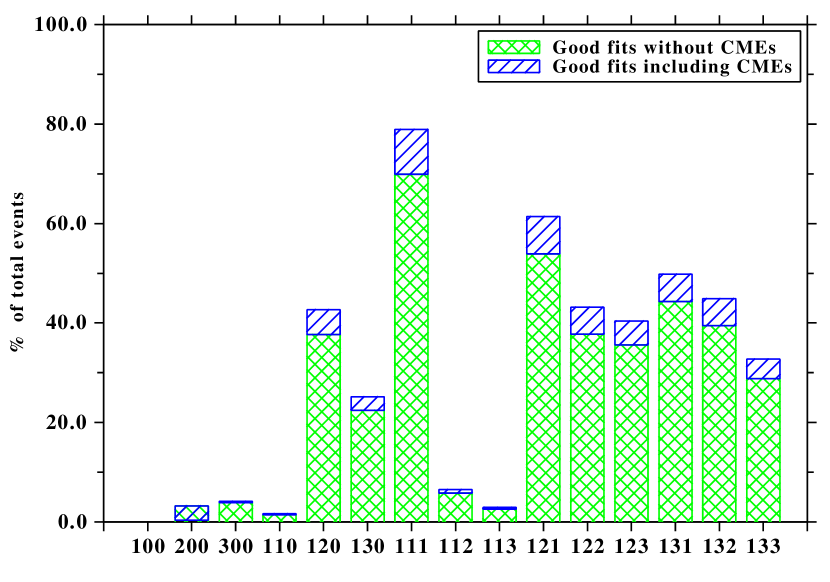
Figure 1: Histogram of the GFs of the entire data set for each fitted (total) distribution $f_{ijk}$. Blue boxes show the additional GFs for the events during CMEs. See Table 1 for the corresponding values.

For the total combined distribution function we introduce the generic notation $f_{t}=f_{ijk}$, where this time indices $i,j$ and $k$ indicate the fitting models. Thus, to avoid further clumsy notation, we use the index $1$ for the AMD, $2$ for the GAK, and $3$ for the RAK, while $0$ indicates that no model is used for the respective component (i.e., for singular or dual fitting models). We write, for example, for a distribution function

$$f_{123}=f_{c,1}+f_{h,2}+f_{s,3}\,,$$ (5)

which means that $f_{123}$ has an AMD core, a GAK halo and an RAK superhalo/strahl. We used the fitting method described in Scherer et al. (2021), which is similar to the one applied by Wilson et al. (2020). The data were fitted with the following combinations of distribution functions: $f_{100}$, $f_{200}$, $f_{300}$, $f_{110}$, $f_{120}$, $f_{130}$, $f_{111}$, $f_{112}$, $f_{113}$, $f_{121}$, $f_{122}$, $f_{123}$, $f_{131}$, $f_{132}$, $f_{133}$. For dual or triple combinations, we always assume that the core distribution is Maxwellian.

To check the quality of the fits we define the relative error

$$E_{i}=\frac{|f_{fit,i}-f_{obs,i}|}{f_{obs,i}}$$ (6)

for each data point $i$, and the mean relative error $<E>$ and its standard deviation $\sigma$ as

$$<E> =\frac{1}{N}\sum\limits_{i=1}^{N}E_{i}\,,$$ (7)

$$\sigma =\sqrt{\frac{1}{N-1}\sum\limits_{i=1}^{N}(<E>-E_{i})^{2}}\,.$$ (8)

For a good fit (GF), see Fig. 1, we require that $<E>\;\leq 0.3$ and $\sigma\leq 0.3$ (Scherer et al., 2021). The events which do not obey this condition or condition (2) for the number densities are rejected. Furthermore, we define the best fit (BF), see Fig. 2, as the minimum of $<E>$ and $\sigma$ of all GFs.

Our analysis covers the Ulysses data from the launch in late 1990 to early 2008. There are in total 324,450 events, including 30,558 events during coronal mass ejections (CMEs), which are taken from Richardson (2014). During CMEs (reduced in number, below 10 $\%$ of the number of events of a certain relevance) the electrons may exhibit a double strahl or two beaming components, sunward and anti-sunward, moving along the closed magnetic field topology. Thus, a double strahl (more or less symmetric) is not reproduced by our models, but it can mimic a suprathermal component with an excess of temperature anisotropy in the direction parallel to the magnetic field. To avoid such a confusing interpretation, the events during CMEs are counted separately in our present analysis. In addition, we have rejected 2,139 events, which violated condition (2). The total number of bad fits is about 20%. Ideally, a data set consists of 400 data points with finite values, but most of the time there are much fewer such points, due to the missing data. If the number of these points is too low, the fits become unreliable, as indicated by the mean error and the standard deviation in the case of rejected fits. The data set is given in keV without any error estimates, thus we were not able to weight the data according to their observational errors, and therefore the weight is always unity.

In Fig. 1 we show the distribution of GFs for all individual distributions functions $f_{ijk}$. The most reduced relevance can be attributed to singular fits, like $f_{100}$, $f_{200}$ or $f_{300}$, with less than $4\leavevmode\nobreak\ \%$ of total events, and those reproducing the halo with a Maxwellian and the strahl with GAK ($f_{112}$ with GFs $<7\leavevmode\nobreak\ \%$) or RAK ($f_{113}$, with GFs $<3\leavevmode\nobreak\ \%$); see Table 1. The highest peak is given by a standard combination of three AMDs, that is, the $f_{111}$ combination, with the ability to provide GFs for about 70 $\%$ of the total data (in the absence of CMEs, with green color). However, GFs are also obtained with all the other combinations involving GAK or RAK for describing the suprathermal populations. These combinations dominate the histogram with representations between 20 % and more than 50 $\%$ of the total number of events: $f_{130}$ with $\sim 22.5\leavevmode\nobreak\ \%$, $f_{133}$ with $\sim 29\leavevmode\nobreak\ \%$, $f_{120}$, $f_{122}$ $f_{123}$ and $f_{132}$, each of them approaching $40\leavevmode\nobreak\ \%$, $f_{131}$ with $\sim 45\leavevmode\nobreak\ \%$, and $f_{121}$ with $\sim 54\leavevmode\nobreak\ \%$; see again Table 1.

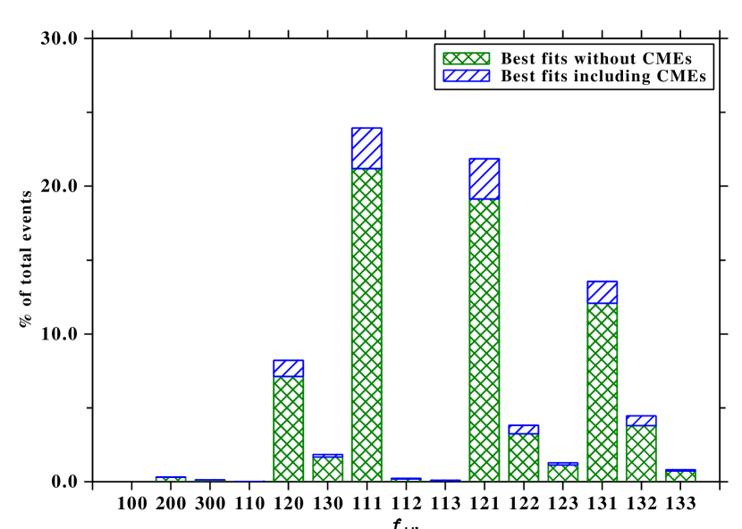
Figure 2: Histogram for the BFs of the entire data set. The green boxes show the BFs without CMEs, the blue boxes show the additional BFs with CMEs. See Table 1 for the corresponding values.

Table 1: Number of events (in $\%$) corresponding to the BFs and to the GFs of all combinations of distribution functions in Figs. 1 and 2.

$f_{ijk}$	BF w/o CMEs	BF	GF w/o CMEs	GF
$f_{100}$	$0.0$	$0.0$	$0.0$	$0.0$
$f_{200}$	$0.3$	$0.3$	$3.2$	$0.3$
$f_{300}$	$0.1$	$0.1$	$3.9$	$4.2$
$f_{110}$	$0.0$	$0.0$	$1.5$	$1.7$
$f_{120}$	$7.1$	$8.2$	$37.7$	$42.7$
$f_{130}$	$1.7$	$1.9$	$22.4$	$25.2$
$f_{111}$	$21.2$	$23.9$	$69.9$	$78.9$
$f_{112}$	$0.2$	$0.2$	$5.8$	$6.5$
$f_{113}$	$0.1$	$0.1$	$2.6$	$2.9$
$f_{121}$	$19.1$	$21.9$	$53.9$	$61.4$
$f_{122}$	$3.2$	$3.8$	$37.7$	$43.2$
$f_{123}$	$1.1$	$1.3$	$35.6$	$40.4$
$f_{131}$	$12.1$	$13.6$	$44.3$	$49.8$
$f_{132}$	$3.8$	$4.5$	$39.5$	$44.9$
$f_{133}$	$0.7$	$0.8$	$28.8$	$32.7$

These results are refined in Fig. 2, which shows the distribution of the BFs for the entire data set (with green for the events without CMEs). The number of BFs (in $\%$) obtained for each combination of distribution functions are given in Table 1, and together sum up to 80.6 % (70.7 % without CMEs) of the total number of events. Thus, each valid event is assigned one of these fitting combinations $f_{ijk}$. It can be seen that 21.2 % of the events without CMEs are best fitted by the $f_{111}$ combination. This is followed at short difference by the $f_{121}$ with 19.1 %, and then by $f_{131}$ with 12.1%, $f_{120}$ with 7.1 %, $f_{132}$ with 3.8 %, $f_{122}$ with 3.2 %, and $f_{130}$ with 1.7 %. Remarkable is the existence of dual core-halo distributions (in the absence of strahl), i.e., $f_{120}$ and $f_{130}$, with almost 9 % of the relevant events. BFs around 1 % are obtained for combinations like $f_{123}$ and $f_{133}$, while singular distributions using GAK (i.e., $f_{200}$) or RAK (i.e., $f_{300}$) have a very reduced presence, with 0.3 % and 0.1 %, respectively. Fitting models involving generalized Kappa distributions, like GAK or RAK, sum up together to 56.7 % of the events (49.5 % without CMEs). It is noteworthy that 59.4 % of the events (52.4 % without CMEs) have the strahl component best reproduced by an AMD, while halos are described by a GAK in about 35 % of the events (30.5 % without CMEs), and by an RKD in about 21 % of the events (18.3 % without CMEs). We must also outline that the most prominent fit combines three AMDs, for 24% of all events (21.2 % without CMEs).

In order to check if the more complicated GAK-halo distribution ($f_{121}$) could be replaced by a simpler RAK-halo distribution ($f_{131}$), we compare the BFs of the $f_{121}$ distribution with the GFs of the $f_{131}$ distribution. Figure 3 displays the mean error of the BFs of the $f_{121}$ distribution against the mean error of GFs of the corresponding $f_{131}$ distribution. It can be seen that about half of the $f_{121}$ distributions can be replaced by the $f_{131}$ distribution and obtaining still a GF. In total we have 63,821 $f_{121}$ BF events, which can be replaced by 37,263 GF events of the $f_{131}$ distribution. Thus, about 58% of the $f_{121}$ distribution could be replaced by the $f_{131}$ distribution. This can be helpful in analytic studies of dispersion relations. Nevertheless, we still have about 42% (26,558) events of the $f_{121}$ distribution for which the fits of the $f_{131}$ distribution give only bad results.

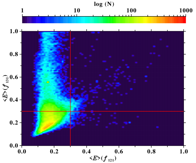
Figure 3: Correlating the mean error of GFs of the $f_{121}$ distribution and the mean error of GFs of the $f_{131}$ distribution. The red line indicates the threshold for a GF.

The total number of bad fits is about 19.4% or 62,843 events, together with 2,139 rejected events (0.66%). These data shall be handled individually (about 20%), because the fit procedure needs to start with a different initial guess, the data sets are too spare to be fitted, or the data cannot be fitted with the above combinations of distribution functions. In the present analysis, from the total number of events we consider the remaining majority of 80 %, or 259,365 events. In the following we discuss the correlation between macroscopic parameters, and concentrate only on the BFs, which are unique. We mainly refer to the most representative combinations like $f_{111},f_{121}$, and $f_{131}$, although the analysis may also take into account the less prominent examples like $f_{120},f_{122}$, or $f_{132}$.

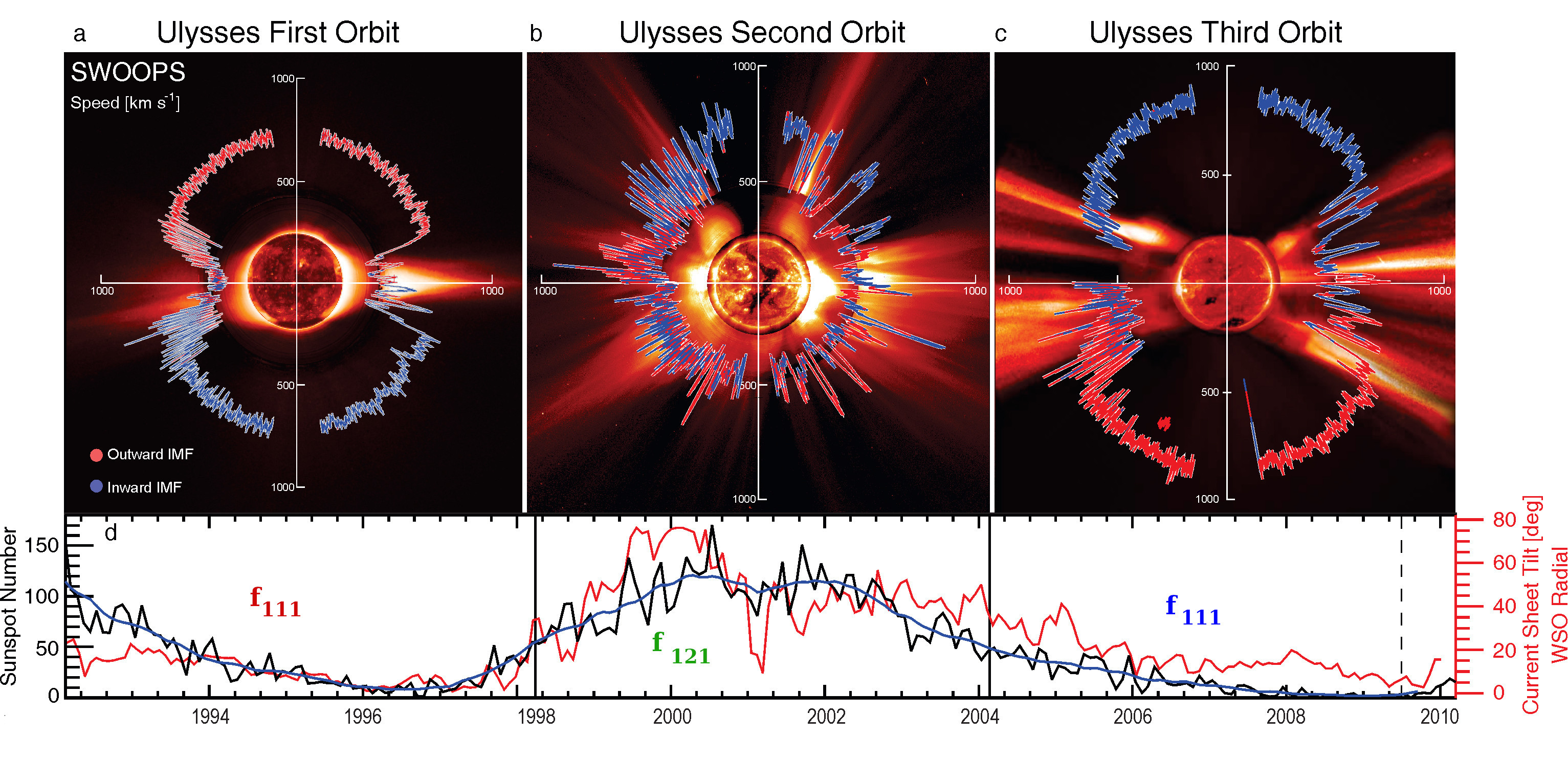
Figure 4: The Ulysses solar wind speeds during time. Adapted from McComas (2008). The three upper panels show the solar wind proton speed as a function of heliographic latitude in a polar coordinate system, during solar minimum (right upper panel), solar maximum (middle upper panel) and again solar minimum (left upper panels).

The corresponding sun spot number (solar activity) is shown in the lower panel, where the black line gives the sunspot number and the red line the tilt angle. Indicated in the lower inlet are the dominant distribution functions during that period to illustrate the solar cycle dependence of the electron distribution functions as shown in Fig. 6.

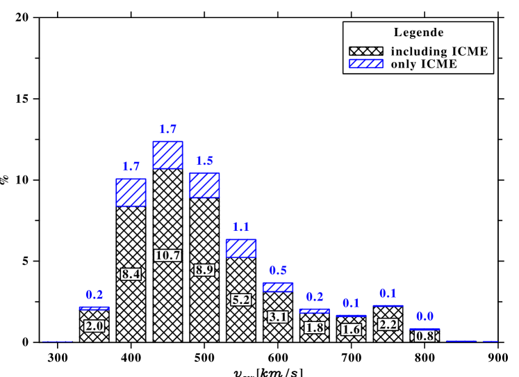
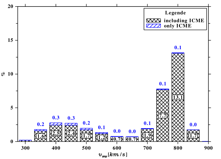
Figure 5: Histograms of the number of events depending on the solar wind speed during the Ulysses mission: from low latitudes $<$$$ (upper panel) and from high latitudes $>$$$ (lower panel).

3 Time and speed variations

We remind the reader of the time and latitude dependence of the solar wind speed along the Ulysses trajectory (McComas et al., 2008), and reprint in Fig. 4 the angular distribution from McComas et al. (2008). It can be seen that during the first and third latitude scan, there are low solar wind speeds below $\approx$$$ latitude and high speeds above $\approx$$$ latitude, and almost no intermediate speeds. This is different during a more active Sun in the second scan, when the speeds scatter over all latitudes.

The difference in solar wind speeds depending on the latitude becomes also evident in Fig. 5, which shows the histograms of the number of events (in %) as a function of the solar wind speed. We split into a part for low latitudes $<$$$ (upper panel) and a part for high latitudes $>$$$ (lower panel). This time the events (and the corresponding values) without CMEs are given in black, while those during CMEs in blue. The gap at intermediate speeds, with about 2.5 % of events, is obvious around $\approx 650$ $\mathrm{k}\mathrm{m}\mathrm{/}\mathrm{s}$. From these histograms one can also observe that the low speeds cluster around 450 km/s at low latitudes near the ecliptic (upper panel), while the high speeds cluster around 750 km/s at high latitudes towards the poles and coronal holes (lower panel). Thus, high speeds are mainly observed during solar minimum (see also McGregor et al., 2011).

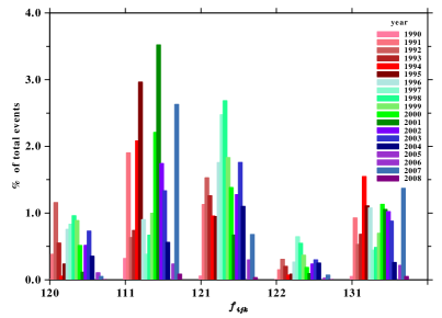
year	$f_{120}$	$f_{111}$	$f_{121}$	$f_{122}$	$f_{131}$	Sum
1990	$0.00$	$0.32$	$0.06$	$0.01$	$0.05$	$0.39$
1991	$0.38$	$1.90$	$1.13$	$0.15$	$0.93$	$3.72$
1992	$1.16$	$0.63$	$1.53$	$0.31$	$0.53$	$3.94$
1993	$0.55$	$0.74$	$1.26$	$0.20$	$0.68$	$2.96$
1994	$0.05$	$2.08$	$0.96$	$0.07$	$1.55$	$3.24$
1995	$0.24$	$2.97$	$0.95$	$0.09$	$1.11$	$4.33$
1996	$0.76$	$0.90$	$1.76$	$0.26$	$1.08$	$3.95$
$\sum^{1996}_{1990}$	$3.14$	$9.54$	$7.65$	$1.87$	$5.94$	$22.44$
1997	$0.83$	$0.38$	$2.48$	$0.64$	$0.45$	$4.98$
1998	$0.96$	$0.67$	$2.68$	$0.55$	$0.49$	$5.41$
1999	$0.89$	$1.00$	$1.83$	$0.37$	$0.70$	$4.46$
2000	$0.52$	$2.21$	$1.38$	$0.19$	$1.13$	$4.48$
$\sum^{2000}_{1997}$	$3.20$	$2.64$	$8.37$	$1.75$	$2.77$	$19.33$
2001	$0.12$	$3.52$	$0.67$	$0.10$	$1.06$	$4.50$
2002	$0.52$	$1.75$	$1.28$	$0.24$	$1.02$	$4.01$
$\sum^{2002}_{2001}$	$0.64$	$5.27$	$1.95$	$0.34$	$2.08$	$8.51$
2003	$0.73$	$1.34$	$1.76$	$0.30$	$0.88$	$4.43$
2004	$0.35$	$0.56$	$1.10$	$0.25$	$0.26$	$2.52$
2005	$0.00$	$0.00$	$0.00$	$0.00$	$0.00$	$0.00$
2006	$0.11$	$0.24$	$0.30$	$0.03$	$0.22$	$0.70$
2007	$0.05$	$2.63$	$0.68$	$0.07$	$1.37$	$3.51$
2008	$0.00$	$0.09$	$0.03$	$0.00$	$0.05$	$0.13$
$\sum^{1008}_{2003}$	$1.24$	$4.86$	$3.87$	$0.65$	$2.78$	$11.29$

Figure 6: The histogram (left panel) and table of relative numbers (left panel) splitted into a yearly basis (right panel). Left panel: Histogram for the BFs of individual years. Inside a distribution function $f_{ijk}$ each bar represents the events per year, from 1990 to 2008. The data for 2005 are missing. The data for 1990 at the beginning of the mission are very sparse, which is also the case toward the end of the mission (after 2005). Right panel: The relative number of events by the BFs of the five most representative distribution functions. For each intermediary row, ”$\sum^{yy}_{yy}$” gives the sum of the years above, and the last column ”Sum” gives the sums of each row. The sum of the last column is 61.57%. Thus, with these five distribution functions we cover approximately 62% of all events (70.7% events without CME).

In Fig. 6 the histogram of Fig. 2 is divided in individual years. This helps us to find the combinations of distribution functions relevant for each orbit of the Ulysses missions, and implicitly for different solar activities. These combinations are also indicated in Fig. 4, in order of their relevance as follows: [$f_{111}$, $f_{121}$, $f_{131}$, $f_{120}$] for the first and third orbits, and [$f_{121}$, $f_{111}$, $f_{131}$, $f_{120}$] for the second orbit. On the other hand, the $f_{111}$ and $f_{131}$ distributions have a dip around the years 1996 to 2000, which is the ascending phase of solar cycle 23 (see Fig. 4), while the $f_{121}$ and $f_{122}$ distributions show a maximum. Unfortunately, that is the only ascending phase which is covered by the Ulysses mission. Therefore, we can only guess that during the ascending phases of a solar cycle, the $f_{121}$ ($f_{122}$) distributions are more appropriate. In two declining phases (that of solar cycle 22 and 23) the distribution functions $f_{111}$ and $f_{131}$ give the most relevant best fits, although $f_{121}$ is also well represented in this case. Thus, in a declining phase of a solar cycle, the electron distributions are better reproduced by three Maxwellians, meaning that they are, individually, closer to thermal equilibrium. Contrarily, in the rising phase, when the solar activity increases, the halo distribution is not well fitted by Maxwellians, meaning that the particles are no longer in thermal equilibrium. The above holds also true for the period around 2002, where the $f_{111}$ and $f_{131}$ distributions have a minimum, and later at 2007 show a maximum (and vice versa for the $f_{121}$ and $f_{122}$ distributions). However, because this is at the end of the misson and no further data are available, we cannot safely conclude that this time dependence is verified by observations. The reason is that the time series only covers parts of a solar Hale cycle, but needed were at least a few such cycles. From a theoretical point of view one may explain the time dependence by the changing magnetic field in the rising phase and the beginning of the solar activity. Thus, the non-equilibrium distributions $f_{121}$ ($f_{122}$) can be caused by an enhanced flare activity. This proposed context needs a more detailed analysis including all spacecraft and solar data, which is far beyond the topic of this work.

4 Case study: temperature anisotropy

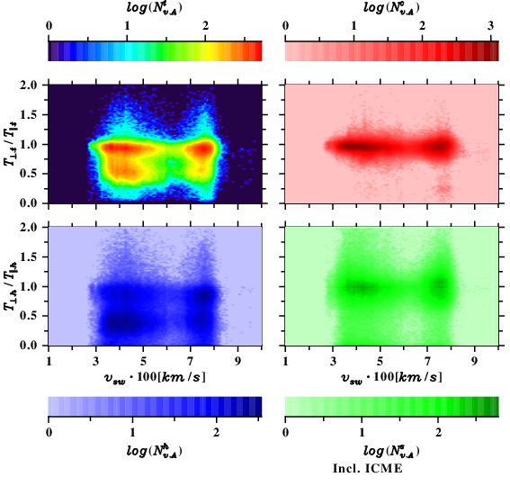
Figure 7: Correlating the solar wind speed (x-axis) given in units of 100 km/s and the temperature anisotropy (y-axis) for all events. The number of events $N_{vA}^{i}$ is given in a logarithmic scale. Here we show the BFs of all fits, while in the following we also show the fits for $f_{111},f_{121}$, and $f_{131}$ distributions. The upper-left panel shows the total anisotropy, the upper-right panel shows that of the core, while the lower-left and lower-right panels that of the halo and strahl, respectively.

The four temperature anisotropies we define as

$$A_{i}=\frac{T_{{}_{\perp},i}}{T_{{}_{\parallel},i}}=\frac{P_{{}_{\perp},1}}{P_{{}_{\parallel},i}}\,,\qquad i\in\{t,c,h,s\}$$ (9)

and additionally, we define the parallel plasma beta as

$$\beta_{\parallel,i}=\frac{8\pi P_{\parallel,i}}{B^{2}},\qquad i\in\{t,c,h,s\}\,.$$ (10)

with magnetic field magnitude $B$. The $\beta_{\perp}$ can be defined, but is not discussed here. See appendix A for further information including the representation method in Fig. 7 to Fig. 10. Furthermore, we only discuss the events without CMEs, and the distributions in the CMEs will be left for future work. We display the total number of events on a rainbow colour-coded scale, while the number of core data is displayed in a reddish, of the halo in a blueish, and of the strahl in a greenish color scale.

Figure 8: Correlating the solar wind speed and the temperature anisotropy without CMEs. The results shown in the columns from left to right are for $f_{all}$, $f_{111}$, $f_{121}$ and $f_{131}$, respectively. Rows from top to bottom display the results for the total, core, halo and strahl distributions, respectively. See text for more details.

4.1 Temperature anisotropy and solar wind speed.

Figures 7 and 8 display the colour-coded binned number of events $N_{vA}^{i},\ i\in\{t,c,h,s\}$ (see Sec. A.1), in a plot with the solar wind speed versus the temperature anisotropy (Eq. 9). In Fig. 7 we correlate temperature anisotropy and solar wind speeds, for the total distribution function of all events, (left-upper panel), and only for the core (right-upper panel), for the halo (left-lower panel), and for the strahl (right-lower panel). In the upper-left panel, four maxima in the number of all events $N_{vA}^{t}$ can be identified: the first one between $v_{sw}=300-500$ km/s and an anisotropy of $A\approx 1$, the second one between $v_{sw}\approx 700$ km/s and $v_{sw}\approx 800$ km/s and $A\approx 1$, and the third and fourth at about the same solar wind speeds, but at lower temperature anisotropies $A\approx 0.5$. The core distribution contributes mainly to the first and second maxima (right-upper panel), while the halo distribution determines the third and fourth maxima, and contributes also to the first and second maximum (left-lower panel). The strahl distribution (right-lower panel) contributes primarily to the first and second maxima. This implies that the temperature anisotropy is mainly caused by the halo and strahl components, while the core distribution is well fitted with an isotropic ($A=1$ temperature) distribution function. The dip at solar wind speeds about $v_{sw}\approx 650$ $\mathrm{k}\mathrm{m}\mathrm{/}\mathrm{s}$ is due to the fact that these speeds are rare (see Figs. 4 and  5).

Figure 8 is structured in a similar way as Fig. 7 and shows a comparison of $f_{all}$ with $f_{111},f_{121}$, and $f_{131}$ (the columns from left to right) by plotting $N_{vA}^{i}$ of the corresponding total, core, halo, and strahl distributions. It can be seen that the $f_{111}$ distributions have maxima at temperature anisotropies around $A=1$ for all four plots: total, core, halo, and strahl. The $f_{121}$ distribution has two maxima along $A\approx 1$ and $A\approx 0.5$, where the former is mainly the contribution from the core, while the latter are contributions from the halo and the strahl. The core of the $f_{121}$ distribution has a similar behavior as that of $f_{111}$ distribution, that is, it scatters mainly around $A=1$. A similar behavior shows the $f_{131}$ distribution, except that the halo does not scatter as much as the halo of the $f_{121}$ distribution. Also, the total anisotropy is smoother for the $f_{131}$ distribution. The total anisotropy for the $f_{111}$ distribution scatters only around $A=1$ (temperature isotropy), while the total of the $f_{121}$ distribution has two maxima around $A=1$ and $A=0.5$, similar to the $f_{131}$ distributions, except that the second maximum around $A=0.5$ is not very pronounced. The dips are again explained by the absence of speeds about $v_{sw}\approx 650$ $\mathrm{k}\mathrm{m}\mathrm{/}\mathrm{s}$ (see above).

The $f_{121}$ distribution shows the strongest scattering in the halo and superhalo component. Nevertheless, because this is the BF, it indicates that there might be another distribution function involved not covered by the fitted AMD, RKD or GAK distributions. The scattering in the fitted halo by the $f_{121}$ distribution might also occur due to the general nature of the GAK. We do not make a closer inspection here, but state that the bulk part of the data is in the maxima of the $f_{121}$ distribution, so that the GAK can be used for fitting.

To conclude this section, we point out that the core has in this analysis a bi-Maxwellian distribution, which can be replaced by an isotropic Maxwell distribution, while the halo and superhalo/strahl are best fitted with anisotropic distributions (here an RAK or GAK). In many cases we can also replace the GAK by the RAK (see the discussion in Sec. 2 above).

Figure 9: Correlating the parallel plasma beta and the temperature anisotropy. Panels are organized as in Fig. 8. See text for more details

4.2 Temperature anisotropy and parallel plasma beta

Figure 9 displays the temperature anisotropy as a function of the parallel plasma beta. In the top panel of first column the total temperature anisotropy of all events is shown. For all distributions, the core events (second row) show small deviations from isotropy and distribute regularly, more or less parallel to the $x$-axis. The halo events (first column, third row) predominantly show an excess of parallel temperature $T_{\parallel,h}>T_{\perp,h}$, revealing a mushroom-like shape, with the leg at $\beta_{\parallel}\approx 0.1$, and the hat widely ranging from very low to high values of $\beta_{\parallel,h}$, e.g., $10^{-4}<\beta_{\parallel,h}<50$. The strahl events (first column, fourth row) are similar, but spread at slightly lower values of $\beta_{\parallel,s}<1$. The distributions of these data are very similar to those obtained by Štverák et al. (2008) with the ecliptic electron data.

The second, third and fourth columns of Fig. 9 display the events fitted by $f_{111}$, $f_{121}$, and $f_{131}$, respectively. It can be seen that the $f_{111}$ distribution has a very weak scattering in all components and is quite similar to the above mentioned plots by Štverák et al. (2008). This is also true for the core events of all other distributions (second row). However, the halo events of the $f_{121}$ and $f_{131}$ distributions show much stronger scattering (third row). Although more restrained, the strahl component (fourth row) show the same variation. For all distributions, the leg is thus a feature mainly resulting from the other distributions not shown here, e.g., $f_{120}$ and $f_{122}$ distributions.

4.3 Temperature anisotropy and $\kappa,\eta_{{}_{\parallel}},\eta_{{}_{\perp}}$, and $\zeta$ parameters

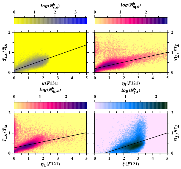
Figure 10: The correlation between the temperature anisotropy and parameters of the halo components of the distributions are displayed. The temperature anisotropy is compared with the $\kappa$ parameter of the $f_{131}$ distribution (left upper panel), and with the $\eta_{{}_{\parallel}}$, $\eta_{{}_{\perp}}$ and $\zeta$ parameters of the $f_{121}$ distribution (right upper panel, left lower panel and right lower panel, respectively). For more explanation see text.

In Fig. 10 we show the correlation between parameters of the halo components of the $f_{131}$ and $f_{121}$ distributions with the temperature anisotropy. The color coding is now given at the top of each panel. In the upper left panel the scattering of the $\kappa$ values of the $f_{131}$ distribution is shown. We can see that $\kappa$ has only values between 0 to about 2.5. It is also evident that the lower the $\kappa$ values are, the lower is the halo temperature anisotropy, that is, the perpendicular temperature is much higher than the parallel one. The reason for $\kappa$ values only below 2.5 can be due to the fact that for higher $\kappa$ values the distribution is comparable to a Maxwellian, and thus the distribution $f_{121}$ approaches $f_{111}$. However, this statement requires more research.

For the $f_{121}$ distribution, the scattering of $\eta_{{}_{\parallel}}$, $\eta_{{}_{\perp}}$ and $\zeta$ parameters is similar to the scattering of $\kappa$ values in the $f_{121}$ distribution, except that $\eta_{{}_{\parallel}}$ has higher values (up to 5, see right upper panel), while $\eta_{{}_{\perp}}$ values have a similar range as $\kappa$ (left lower panel). The $\zeta$ parameter (right lower panel) is similar to the $\eta_{{}_{\perp}}$ parameter. The $f_{131}$ halo component shows also an increased scattering in the anisotropy around $\eta_{{}_{\parallel}}=0$, $\eta_{{}_{\perp}}=0$ and $\zeta=0$, which can be caused by the fitting procedure due to the small values of the corresponding parameters.

We computed a linear regression for the data shown in Fig. 10 via

$$A(x)=\frac{T_{{}_{\perp}h}}{T_{{}_{\parallel}h}}=ax+b\,,$$ (11)

where $x\in\{\kappa,\eta_{{}_{\parallel}},\eta_{{}_{\perp}}.\zeta\}$. The values for the fits are listed in Table 2.

Table 2: The fit values for the linear regression (Eq. 11) as shown in Fig. 10.

$A(x)$	a	b
$A(\kappa)$	0.25	0.11
$A(\eta_{{}_{\parallel}})$	0.16	0.19
$A(\eta_{{}_{\perp}})$	0.15	0.27
$A(\zeta$)	0.23	-0.16

The linear regression is quite good for $A(\kappa)$, but for $A(\eta_{{}_{\parallel}})$ and $A(\eta_{{}_{\perp}})$ the events form a curve asymptotically approaching $A=1$. The fit for $A(\zeta)$ runs through a cloud, which clusters around the linear regression and scatters toward higher anisotropies. Nevertheless, the simplified regressions can help to study the temperature anisotropy in the halo with increasing values of $\kappa,\eta_{{}_{\parallel}},\eta_{{}_{\perp}}$ and $\zeta$.

5 Conclusions

In the present work we used a 2D fitting method, which accounts for different temperatures parallel and perpendicular with respect to the background magnetic field, to fit electron velocity distributions obtained during the Ulysses mission. In doing so, we used a triple model to fit the core, halo and superhalo/strahl populations within the total distribution. As model functions we applied an anisotropic Maxwellian distribution (AMD), a generalized anisotropic Kappa (GAK) and a regularized anisotropic Kappa (RAK) distribution. Our findings indicate a time dependence of the electron distributions on the solar cycle. Unfortunately, the data series is not long enough to solidly confirm such a behavior. Nevertheless, the results suggest that in a declining phase of a solar cycle, the individual electron distributions are best described by three Maxwellians, meaning that they are in thermal equilibrium. In the ascending phase, when the solar activity increases, the halo distribution is not well fitted by a Maxwellian, which means that the particles are out of thermal equilibrium. This behaviour deserves more attention and should be be combined with other spacecraft data. However, due to the unique solar polar orbit of Ulysses and the fact that most of the other spacecraft are in the ecliptic (HELIOS) or close to the Sun (Parker Space Probe, Solar Orbiter), one has in principle to subtract distance and latitude effects.

While the core distribution can most likely be fitted with an isotropic Maxwell distribution as the temperature anisotropy is close to 1 (see the reddish color panels in the figures in Sec. 4), the halo and superhalo/strahl (the blueish and greenish colo panels) are best fitted with anisotropic distributions (here with an RAK or a GAK. In many cases we can also replace the GAK by the simpler RAK, resulting in a slightly worse fit (see Fig. 3).

The parallel plasma beta correlation with the temperature anisotropy is similar for the three distributions $f_{111},f_{121}$, and $f_{131}$, but shows a stipe for the halo distribution in the sample of all distributions. We also showed the correlation between the temperature anisotropy and the $\kappa$ parameter of the $f_{131}$ distribution as well as the $\eta_{{}_{\parallel}}$, $\eta_{{}_{\perp}}$ and $\zeta$ parameters of the $f_{121}$ distribution. The temperature anisotropy shows almost a linear dependence on $\kappa$ with increasing values of $\kappa$, and the temperature anisotropy becomes more isotropic. For the GAK parameters ($\eta_{{}_{\parallel}},\eta_{{}_{\perp}},\zeta$) we found also a linear dependence of the temperature anisotropy.

Finally, we want to direct the attention to Fig. 4 which shows that during a solar cycle also the type of the distribution functions changes from mainly a $f_{111}$ type near solar minimum to a more general $f_{121}$ type close to solar maximum and back to $f_{111}$ for the next minimum phase. These results demonstrate that the multi-distribution function fitting of velocity distributions has a significant potential to advance our understanding of the solar wind kinetics and, therefore, deserves further quantitative analyses.

The data sets were derived from sources in the public domain, available at http://ufa.esac.esa.int/ufa/#data/.

Appendix A The pressure and temperature moments

We repeat here shortly the definitions given in Paschmann et al. (1998) and Scherer et al. (2021). The partial parallel and perpendicular thermal pressures are given as follows:

$$P_{th}= \frac{1}{3}\left(\sum\limits_{i}P_{\parallel,i}+2\sum\limits_{i}P_{\perp,i}\right)\qquad i\in\{c,h,s\}$$ (12)

$$\Rightarrow$$

(13)

The total pressure $P_{tot}$ is the sum of the thermal pressure plus (twice) the ram pressures (see Scherer et al. (2021) for further explanation).

The respective temperatures are given by the ideal gas law as

$$T_{\parallel,i} \equiv\frac{P_{\parallel,i}}{k_{B}n_{i}}\,,\qquad\qquad T_{\perp,i}\equiv\frac{P_{\perp,i}}{k_{B}n_{i}}\,,\qquad i\in\{c,h,s\}$$ (14a)

with $$k_{B}$$ denoting Boltzmann’s constant, and

$$T_{\parallel,t}=\sum\limits_{i}\frac{n_{i}T_{\parallel,i}}{n_{t}}\,,\qquad\qquad T_{\perp,t}=\sum\limits_{i}\frac{n_{i}T_{\perp,i}}{n_{t}}\,,$$ (14b)

where number density $$n_{t}$$ is given by

$$n_{t}=\sum\limits_{i}n_{i}\,,\qquad i\in\{c,h,s\}\,.$$ (14c)

A.1 Representation method

In the graphical representations we divide the $x$- and $y$-axis in 100 sub-intervals $\Delta x_{i}$ and $\Delta y_{j}$, and compute the total number of events (data points) $N_{all}$ in each interval $N_{i,j}/(\Delta x_{i}\Delta y_{j})$ via

$$N_{all}=\sum\limits_{i,j}N_{i,j}/(\Delta x_{i}\Delta y_{j})\,.$$ (15)

As stated above, we only discuss the macroscopic parameters for the most relevant distribution functions, according to their BFs, that is, $f_{all},f_{111},f_{121}$, and $f_{131}$, where $f_{all}$ are all the BFs including all distributions $f_{ijk}$. We always show first the total, core, halo and superhalo/strahl moments for $f_{all}$, and then we show how the moments for the single distributions $f_{111},f_{121}$ and $f_{131}$ contribute to $f_{all}$.