CorAl: Introspection for Robust Radar and Lidar Perception in Diverse Environments Using Differential Entropy

Abstract

Robust perception is an essential component to enable long-term operation of mobile robots. It depends on failure resilience through reliable sensor data and pre-processing, as well as failure awareness through introspection, for example the abaility to self-assess localization performance. This paper presents CorAl: a principled, intuitive, and generalizable method to measure the quality of alignment between pairs of point clouds, which learns to detect alignment errors in a self-supervised manner. CorAl compares the differential entropy in the point clouds separately with the entropy in their union to account for entropy inherent to the scene. By making use of dual entropy measurements, we obtain a quality metric that is highly sensitive to small alignment errors and still generalizes well to unseen environments. In this work, we extend our previous work on lidar-only CorAl to radar data by proposing a two-step filtering technique that produces high-quality point clouds from noisy radar scans. Thus we target robust perception in two ways: by introducing a method that introspectively assesses alignment quality, and applying it to an inherently robust sensor modality. We show that our filtering technique combined with CorAl can be applied to the problem of alignment classification, and that it detects small alignment errors in urban settings with up to 98% accuracy, and with up to 96% if trained only in a different environment. Our lidar and radar experiments demonstrate that CorAl outperforms previous methods both on the ETH lidar benchmark, which includes several indoor and outdoor environments, and the large-scale Oxford and MulRan radar data sets for urban traffic scenarios The results also demonstrate that CorAl generalizes very well across substantially different environments without the need of retraining.

I Introduction

For mobile robots to be truly resilient to possible failure causes, during long-term hands-off operation in difficult environments, robust perception needs to be addressed on several levels. Robust perception depends on failure resilience as well as failure awareness. Several stages of the perception pipeline are affected: from the sensory measurements themselves (sensors should generate reliable data also under difficult environmental conditions), via algorithms for registration, mapping, localization, etc, to introspection (by which we mean self-assessment of the robot’s performance).

This paper presents novel work on robust perception that addresses both ends of this spectrum, namely CorAl (from “Correctly Aligned?”); a method to introspectively measure and detect misalignments between pairs of point clouds. In particular, we show how it can be applied to range data both from lidar and radar scanners; which means that it is well suited for robust navigation in all-weather conditions.

Lidar sensing is, compared to visual sensors, inherently more unaffected by poor lighting conditions (darkness, shadows, strong sunlight). Radar is furthermore unaffected by low visibility due to fog, dust, and smoke. However, radar as a range sensor has rather different characteristics than lidar, and interpreting radar data (e.g., for localization) has been considered challenging due to high and environment-dependent noise levels, multi-path reflections, speckle noise, and receiver saturation. In this work we demonstrate how radar data can be effectively filtered to produce high-quality point clouds; and how even small misalignments can be reliably detected.

Many perception tasks, including odometry estimation [1], localization [2], and sensor calibration [3], rely on point cloud registration. However, registration sometimes provides incorrect estimates; e.g., due to local minima of the registration cost function [4], uncompensated motion distortion [5], rapid rotation (leading to poor initial pose estimates) [6], or when the registration problem is geometrically under-constrained [7, 8].

Consequently, it is essential to equip these methods with failure awareness by measuring alignment quality so that misaligned point clouds can be rejected or re-aligned. While a number of measures of alignment quality already exist, it is typically not easy to set a threshold to detect poor alignments that can be used in different environments – as we also demonstrate in our experimental validations (see Secs. IV and V). A particular benefit of the CorAl method is that it generalizes well, so that if it has been trained in one environment, the same parameters can be used in other, unseen, environments.

Some examples of methods that have been used in practice to assess the alignment quality include point-to-point or point-to-plane distances [9, 10], point-to-distribution [11, 12] or distribution-to-distribution [13, 14] likelihood estimates, mean map entropy [15] or dense radar-image comparison [16]. However, except for some notable exceptions [12, 17], few studies in the literature have specifically and methodically targeted the measurement of alignment correctness.

Our method, CorAl, is well-grounded in information theory and gives an intuitive alignment correctness measure. Fig. 1 shows the general outline of the method, and Fig. 2 illustrates the output per-point alignment measure for a pair of point clouds. CorAl computes the average differential entropy in two point clouds, exploiting the difference when the entropy is computed for each point cloud separately, compared to the union of the point clouds. For well-aligned point clouds, the joint and the separate point clouds will have similar entropy. In contrast, misaligned point clouds tend to “blur” the scene, which can be measured as an increase in joint entropy as depicted in Fig. 3. A key idea is to estimate the entropy inherent in the scene from the entropy in the separate point clouds, which enables CorAl to accurately assess quality in a range of different environments. In short, our previous contribution was an intuitive and simple measure of alignment correctness between point cloud pairs that generalizes across environments and highlights regions of misalignment. This paper extends our previous work on CorAl [17] by showing how it can be applied to FMCW (frequency-modulated continuous wave) radar data, thus pushing further towards truly robust perception, and includes quantitative evaluations on two new large-scale benchmarks and four new baselines. In summarize, we present the following new contributions:

• The first investigation (to our knowledge) that systematically evaluates alignment correctness classification using radar-based feature extraction and quality metrics without the aid of auxiliary sensors.

• We include 4 new baselines based on recent research within spinning radar odometry.

• A novel radar filtering strategy that allows CorAl to operate on noisy radar data, enabling alignment classification of small errors with high accuracy compared to previous radar feature extraction methods in urban traffic settings.

• An ablation study that investigates parameter importance and how practical factors such as error magnitude and variation in distance between scans influence classification performance.

• A cross-environment study that demonstrates that CorAl generalizes to new environments without retraining.

Figure 1: CorAl, depicted in blue, operates on a pair of point clouds $\mathcal{P}_{a},\mathcal{P}_{b}$ and can classify misalignment ($y_{pred}$) by comparing the differential entropy in the point clouds separately and jointly. Additionally, CorAl outputs a per-point quality measure $\mathbf{q}$ that highlights misaligned parts.

(a)

(b)

(c)

(d)

Figure 2: Top: Differential entropy in point clouds separately. Colors range from red (low entropy) to blue and violet (high entropy). Bottom: The joint point cloud ($\mathcal{P}_{a}\cup\mathcal{P}_{b}$) colored by per-point quality measure $q_{k}(\mathcal{P}_{a},\mathcal{P}_{b})$ when aligned (c) and when misaligned (d). Blue and red indicate alignment and misalignment respectively.

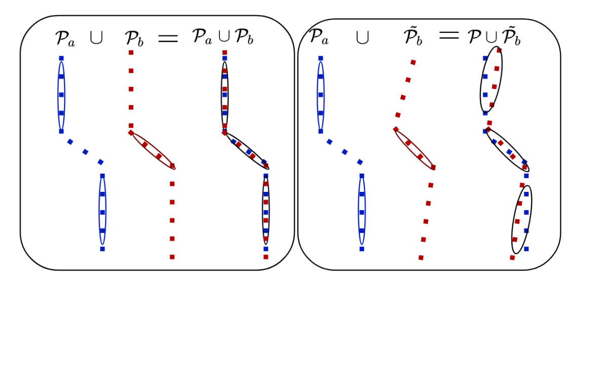
Figure 3: Example how uncertainty (entropy) is preserved when joining aligned point clouds $\mathcal{P}_{a}\cup\mathcal{P}_{b}$ (left), but increases when joining misaligned point clouds (right). The entropy for aligned point clouds should be similar to the entropy in the separate point clouds and can be used when quantifying alignment quality.

II Related work

II-A Cost functions for scan registration

In practice, it is common to use the cost function of a scan registration method to estimate the alignment quality after registration.

One well-used alignment measure is the root-mean-squared (RMS) point-to-point distance, truncated by some outlier rejection threshold. This is also the function that is minimized by iterative closest point registration [18, 10]. However, this measure has been shown to be highly sensitive to the environment and the choice of the outlier threshold [19, 12] when trying to detect small errors. Consequently, this is a poor measure for alignment correctness classification.

Another common alternative is the point-to-line distance [9, 10] or – as a generalization – a point-to-distribution [11, 20] or distribution-to-distribution [13] measure; where local surface descriptors are computed using the spatial distribution of points within a neighborhood. In a similar vein, Liao et al. [14] propose distribution-to-distribution registration based on fuzzy clusters, and estimate coarse alignment quality via the dispersion and disposition of points around fuzzy cluster centers. These methods have also been shown to generalize poorly for assessing 3D lidar scan alignment in different environments [17].

II-B Fault detection and uncertainty estimation

Going beyond merely setting a threshold for the registration cost function, there are also some methods that have been devised specifically for fault detection and uncertainty estimation.

Huan et al. [21] presented a failure detection based on logistic regression and using point cloud overlap, differences between 2d point cloud projections and mean and deviation of nearest point distance and normal directions. They show that various metrics can be combined for increased accuracy, however the work does not explicitly focus on detecting small errors and instead includes errors up to 5 m.

Makadia et al. [22] use consistency between normals (“plane-to-plane“) as a post-registration alignment measure, where normals are computed from voxelized versions of two point clouds. In an independent evaluation [12], this method was found to perform poorly in unstructured outdoor environments.

Nobili et al. [7] proposed a method to predict alignment risk prior to registration by combining overlap information and an alignment metric that quantifies the geometric constraints in the registration problem. Their alignment metric is based on point-to-plane residuals and has been evaluated in structured scenes with planar surfaces. In contrast, the method we propose in this paper can operate well even in unstructured environments. Additionally, our method seeks to estimate the alignment after registration has been completed to introspectively measure the registration success, as opposed to predicting the risk prior to registration.

Akai et al. [23] estimate reliability of vehicle localization from grid map and laser scan data, using a convolutional neural network (CNN). In our work, we are interested in alignment classification without prior knowledge for pairs of point clouds. Aldera et al. [24] learn detection of odometry failures in challenging conditions using weak supervision from IMU or GPS. Their method analyzes eigenvectors of a pairwise compatibility matrix which contains scores between point correspondences. Finally, Sundvall and Jensfelt [25] propose a method for fault detection with redundant positioning systems. In contrast, our method operates on lidar or radar without the need for any additional sensors during deployment and uses odometry or optionally ground truth during training.

A family of methods assessing alignment uncertainty based on an estimate of the pose covariance can be found in [26, 27, 28, 29, 30, 11, 31]. Some of these use a Monte Carlo method and estimate uncertainty by sampling registrations in a region [27]. For mobile robotics, sampling strategies are tedious and unpractical. Other methods compute covariance in closed form based on the Hessian of the quality metric [30, 11] or from pose samples weighted by dense correlation [31, 16]. However, it is not generally possible to define a fixed set of covariance thresholds to distinguish good from bad alignments.

Bogoslavskyi and Stachniss [32] define a quality metric that takes into account free-space information, and use it to measure alignment error between range images of segmented 3D objects in a controlled experiment. Rather than focusing on objects, our method aims to classify the alignment quality of observed scenes in different environments. Additionally, their method operates on range images, which might not be easily available, while our method operates on unorganized point clouds.

Some methods work on the scale of a full map, rather than individual scans. Chandran-Ramesh and Newman [33] convert a point cloud map into plane patches and train a conditional random field to detect plausible and suspicious plane configurations. This method is not directly applicable for assessing pairwise point cloud alignment. Droeschel and Behnke [15] compute mean map entropy to measure the “crispness” of a point cloud map, with the aim to evaluate accuracy of scan registration in lieu of ground truth pose data. Our work is inspired by this measure but, as further detailed and demonstrated below, mean map entropy does not generalize between structured and semi-structured environments.

II-C Feature extraction and quality assessment for spinning radar

Lidar is a well-investigated sensor modality in robot perception. Spinning FMCW radar is an alternative modality that has been receiving more attention in recent years, due to it being resilient to low-visibility conditions. However, due to its challenging noise characteristics, how to efficiently interpret the data for robot perception is still considered an open research question. Hence, in our investigation of radar we include both feature extraction and quality assessment. Radar-based methods that use alignment quality measures can be categorized into dense methods [16, 34, 35], which operate on raw radar images and do not explicitly perform data association, and sparse methods [36, 37, 38, 39, 40, 41, 42, 43, 1], which compute alignment quality using keypoint locations, shape and descriptors over a correspondence set. Previous sparse methods use (weighted) Point-to-Point [39, 41, 42], Point-to-distribution [43] and Point-to-Line [1] metrics. Key points can be extracted via SURF, blob detection [36], gradient-based feature detectors [41, 42], by a set of oriented surface points [1] or distributions [43] using a grid-based approach, or by semi-supervised [39] and unsupervised [39, 40] deep learning methods.

While these methods for feature extraction and alignment quality have been used as objective functions for the purpose of estimating odometry, it is currently not known to which extent these metrics can be used for alignment correctness classification. Previous work shows that the performance of deep learning-based odometry methods decreases in new environment types [16, 38]. However, some methods have been successful in estimating odometry and performing SLAM in widely different environments without deep learning and even without parameter tuning [1, 36]. In this paper, we show that learning-free feature extraction methods can produce stable key points over multiple environment types, and are suitable for alignment correctness classification in diverse environments. Hence, we can forego (deep) learning for feature extraction and only use logistic regression at the classification stage to learn linear decision boundaries, which ultimately only requires two parameters to be trained.

II-D Comparative studies of alignment assessment

Most of the methods above have been used in a more or less ad-hoc manner. Few systematic evaluations and comparative studies have been made on investigating their general capability for the task of alignment classification between point clouds pairs, i.e. to detect aligned vs. misaligned ones. Two evaluations in this direction were presented by Almvqvist et al. [12] and in on our previous work CorAl [17] where a range of quality metrics was used to train classifiers using logistic regression. Almqvist et al. explored alignment classifiers based on point-to-point distances as well as a number of other methods [10, 44, 11, 33, 45, 19], and investigated how to combine the measures with AdaBoost into a stronger classifier. The classifiers were evaluated on two outdoor data sets, and although the best ones reached almost 90 % accuracy for the hardest cases on each data set individually, accuracy drops to around 80 % when cross-evaluating between the data sets. In their evaluations, the NDT score function [11] proved to be the best individual measure for alignment assessment. The combined AdaBoost classifier did not have significantly higher accuracy, but reduced parameter sensitivity. Our previous work confirms the finding by Almqvist: that detecting small alignment errors in a diverse range of environments without retraining is challenging.

III CorAl method

Our work takes inspiration from Droeschel and Behnke [15] who used differential entropy measurements to assess map quality. The differential entropy measures the uncertainty or surprisal of a continuous variable, in their case for (3-dimensional) variables $X\in\mathbb{R}^{3}$ with multivariate Gaussian distribution $X\sim\mathcal{N}_{3}(\mathbf{\mu},\,\mathbf{\Sigma})$. Distributions are approximated by the sample mean and covariance of local point distribution within a radius $r$. In their work, they compute the “Mean-Map-Entropy” (MME), defined as the average per-point differential entropy over a set of point clouds, and use the measure to compare methods for lidar map refinement algorithms without the need for ground truth measurements and without imposing planar assumptions. As the entropies measure surprisal, everything else being equal, a lower MME measure can be interpreted as less surprisal or crisper point clouds and indicate the success of map refinement. While MME is suitable for and has been used to quantify relative alignment improvement [46, 47], the metric additionally depends on sensor noise and sample density and is highly dependent on scene geometry. Consequently, and as confirmed by our evaluation, the metric does not generalize over, e.g. structured and semi-structured environments. For that reason, we overcome sensitivity to variation in scene geometry by making use of dual entropy measurements computed 1) in point clouds separately and 2) in the joint point cloud. Intuitively, when joining a well-aligned point cloud pair, the entropy (or the blur) found in the joint point cloud should not increase compared to the entropy found in the separate point clouds, and instead, remain close to constant. In contrast, when joining point clouds with small misalignments, the joint entropy (blur) tends to increase compared to the separate entropy. By making use of dual differential entropy measurements, our method can account for the scene appearance and detect small alignment errors. Additionally, the measurements enable generalization to substantially different environments without retraining.

III-A Assumptions and definitions

CorAl operates on 2D or 3D point cloud pairs $\mathcal{P}_{a}$, $\mathcal{P}_{b}$ acquired by a range sensor such as lidar or radar. Points $\mathbb{p}_{k}\in\mathcal{P}$ are given in a common fixed world frame in $\mathbb{p}_{k}\in\mathbb{R}^{2}$ or $\mathbb{p}_{k}\in\mathbb{R}^{3}$. CorAl learns a linear decision boundary to separate aligned vs misaligned point-cloud pairs based on features extracted without learning. During the learning phase, point clouds are assumed to be correctly aligned by an accurate ground truth or odometry system and free of distortions from motion. We aim to detect small alignment errors. Detecting large errors e.g. $>1$ m in large-scale-urban or larger than $>0.4$ m within indoor environments is generally not considered challenging for traditional metrics such as point-to-point or point-to-line metrics, thus, it is not the focus of our work. For notation, we define the joint point cloud $\mathcal{P}_{j}=\mathcal{P}_{a}\cup\mathcal{P}_{b}$; i.e., all points in $\mathcal{P}_{a}$ and $\mathcal{P}_{b}$ together.

III-B Joint and separate entropy measurements

In order to compute the differential entropy around a single point, we first compute the sample covariance $\mathbb{\Sigma(p}_{k})$ from all points within a radius $r$ around $\mathbb{p}_{k}$. The differential entropy can then be computed from the determinant of the sample covariance according to:

$$h_{i}(\mathbb{p}_{k})=\frac{1}{2}\ln((2\pi e)^{N}\det(\Sigma(\mathbb{p}_{k}))),$$ (1)

for a multivariate normal distribution with dimension $N$. The property of this metric can be visually understood from Fig. 2a where each point is colored according to the differential entropy. The metric serves as a geometric descriptor that describes the local geometry with a single value; the differential entropy.

The MME can then be computed by averaging Eq. 1 over the joint point cloud $\mathcal{P}_{j}$; i.e., computing the sum and then dividing by the number of terms as shown in Eq. 2 and Eq. 3,

$$H_{i}(\mathcal{P}_{i})=\sum_{k=1}^{|\mathcal{P}_{i}|}h_{i}(\mathbb{p}_{k}),$$ (2)

$$H_{\mathrm{joint}}=(MME)=\frac{H_{j}(\mathcal{P}_{j})}{|\mathcal{P}_{j}|}=\frac{H(\mathcal{P}_{a}\cup\mathcal{P}_{b})}{|\mathcal{P}_{a}|+|\mathcal{P}_{b}|},$$ (3)

where $|\mathcal{P}_{i}|$ is the number of points in the point cloud $\mathcal{P}_{i}$. We extend this formulation by additionally computing the entropy in $\mathcal{P}_{a},\mathcal{P}_{b}$ separately:

$$H_{\mathrm{sep}}=\frac{H_{a}(\mathcal{P}_{a})+H_{b}(\mathcal{P}_{b})}{|\mathcal{P}_{a}|+|\mathcal{P}_{b}|},$$ (4)

and obtain our quality metric by subtracting the average differential entropy from the joint:

$$Q(\mathcal{P}_{a},\mathcal{P}_{b})=H_{\mathrm{joint}}(\mathcal{P}_{j})-H_{\mathrm{sep}}(\mathcal{P}_{a},\mathcal{P}_{b}).$$ (5)

The CorAl quality metric is hence  the difference in differential entropy. The CorAl quality can also be given on a per-point level by

$$q_{k}(\mathbb{p}_{k})=h_{j}(\mathbb{p}_{k})-h_{i}(\mathbb{p}_{k}),$$ (6)

where $i$ is the point cloud ($a$ or $b$) $\mathbb{p}_{k}$ originates from. While the differential entropy in Eq. 1 varies according to the shape of the environment, the per-point entropy difference in Eq. 6 has the property of being close to zero when point clouds are well aligned and increase with misalignment as depicted in Fig. 2c. The corresponding function surface of the quality measure $Q(\mathcal{P}_{a},\mathcal{P}_{b})$ is depicted in Fig.  4, which demonstrates how the score increases when displacing one of the point clouds in translation and orientation.

(a) Top view of the first two aligned point clouds $\mathcal{P}_{a}$(blue) and $\mathcal{P}_{b}$(red) in the ETH “stairs” dataset.

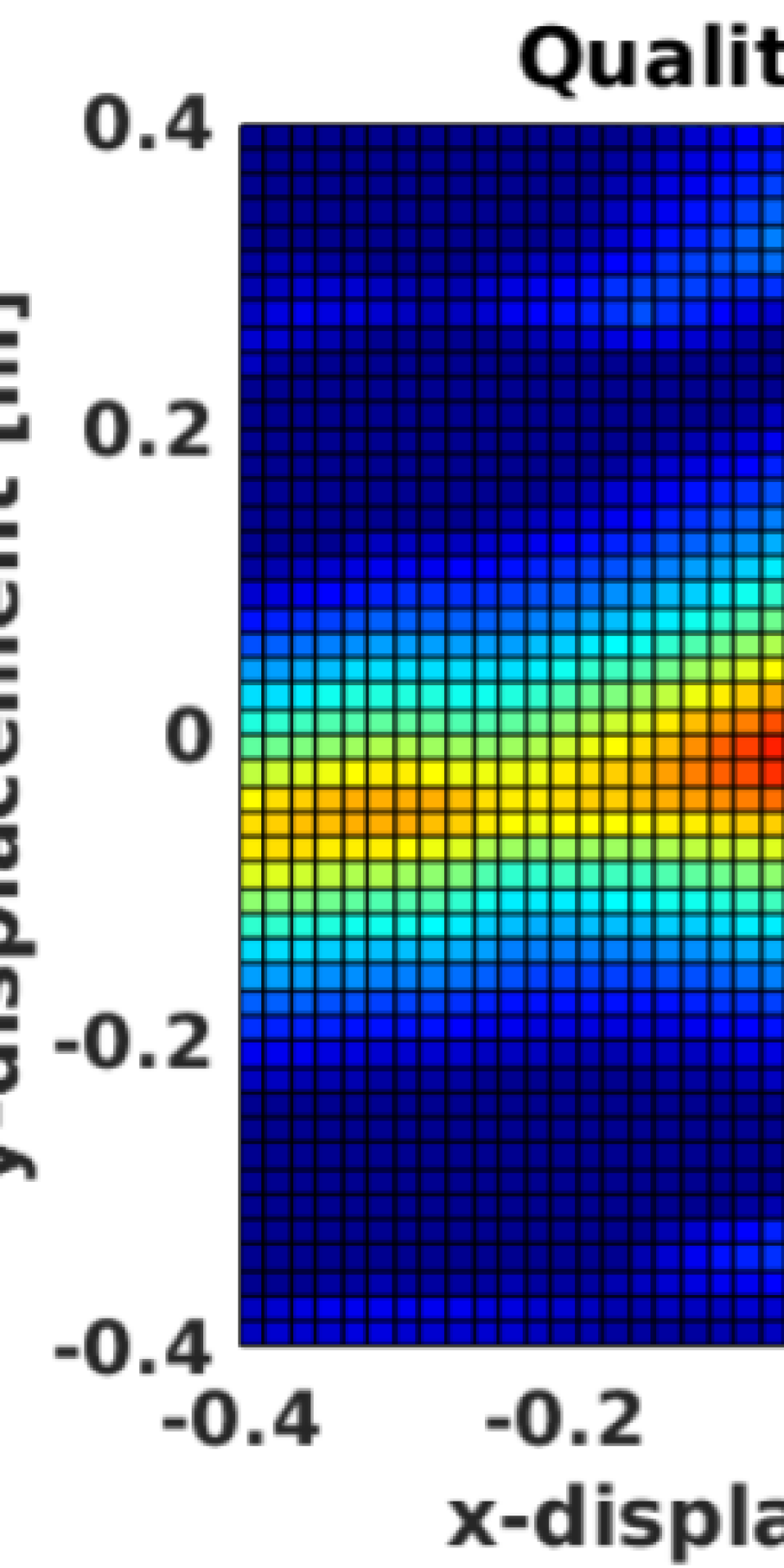
(b)

Figure 4: $Q$ has a minimum at the true position. The steepness of the surface around the true alignment indicates that CorAl is sensitive to small misalignments.

Well-aligned point clouds $\mathcal{P}_{a}\cup\mathcal{P}_{b}$ acquired in structured environments have low differential entropy for most query points $\mathbb{p}_{k}$. This is reflected by low values for the determinant of the sample covariance. As the determinant can be expressed as the product of the eigenvalues of the sample covariance $\det(\mathbb{\Sigma(\mathbb{p}}_{k}))=\lambda_{1}\lambda_{2}\lambda_{3}$, we see that the measure is sensitive to an increase in the lowest of the eigenvalues when larger eigenvalues are constant. For example, the entropy of points on a planar surface is represented with a flat distribution with two large ($\lambda_{1},\lambda_{2}$) and one small ($\lambda_{3}$) eigenvalue. Misalignment changes the point distribution in the joint point cloud from flat to ellipsoidal, which can be observed as an increase of the smallest eigenvalue $\lambda_{3}$. This makes the measure sensitive to misalignment of planar surfaces while generalizing well to other geometries. As shown in the evaluation, the CorAl measure can capture discrepancies between point clouds regardless of whether these are due to rigid misalignments or distortions that can occur when scanning while moving (e.g., because of vibrations or sensor velocity estimation errors). That means that the method may also be overly sensitive when used together with a registration method or odometry framework that does not compensate movement distortion or has a low accuracy.

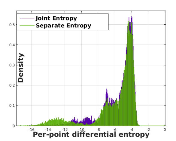
(a) Aligned point clouds: differential entropy distributions are similar.

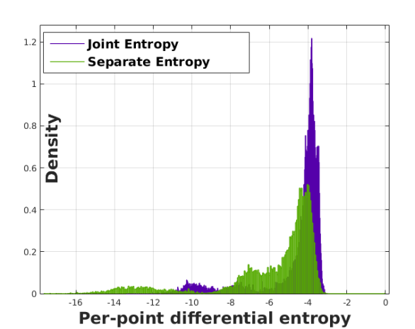
(b) Misaligned point clouds: joint differential entropy is higher.

Figure 5: Probability distribution of per-point entropy Eq. 1 for joint and separate point clouds when aligned (a) and misaligned (b). Aligned point clouds have similar joint and separate entropy distributions. For misaligned point cloud pairs, the distribution of joint entropy is shifted compared to the separate entropy distribution. Joining misaligned point clouds tend to blur the scene, which can be observed by an entropy increase. An exception can be seen in (a), within region $(-12,-8)$, where entropy mistakenly increases when joining aligned point clouds as described in  III-C.

III-C Dynamic radius selection and outlier rejection

For well-aligned point clouds, the quality measure $Q$ has values close to zero. In this case, the distribution of per-point differential entropies in the joint and separate point clouds are similar. The per-point entropy distributions are depicted in Fig. 5a for a set of aligned and misaligned point cloud pairs when using fixed radius for computing entropies. Unfortunately, the entropy in Eq. 1 is numerically unstable when the determinant of the covariance $\det(\mathbb{\Sigma}(\mathbb{p}_{k}))$ is ill-conditioned, hence a small increase of the determinant causes a large increase of the entropy. Accordingly, the lowest measured entropies can increase a lot (which mistakenly indicates misalignment) even when joining well-aligned point clouds as depicted in Fig. 5a.

One case where entropy mistakenly increases is when a 3d lidar observes floor regions with sparse ring patterns (due to space between vertical beams of the sensor). In the separate point clouds, the sparse rings give rise to ellipsoidal covariances (low entropy) with high uncertainty along the ring direction and low in the other directions. In the joint point cloud, the sparsity between rings is reduced, the computed covariances are instead planar according to the floor plane, with two high eigenvalues and one low, and therefore have a higher entropy.

Ill-conditioned covariances occur where point density is low, typically for solitary points or far from the sensor where the radius $r$ is not large enough, e.g., to include multiple “lidar rings” within one entropy measurement, as in the example described above.

The ill-conditioned entropies can be mitigated by increasing the radius $r$ or making use of the options described below. Obviously, for a set of point cloud pairs, the parameters are typically well-calibrated (and ill-conditioned entropies have been mitigated) if CorAl can separate between aligned and misaligned point clouds. This occurs when the joint $H_{j}$ and separate $H_{sep}$ entropies are linearly separable. The parameter can be calibrated by maximizing the ratio:

$$Q_{s}=Q_{misaligned}(\mathcal{P}_{a},\mathcal{P}_{b})/Q_{aligned}(\mathcal{P}_{a},\mathcal{P}_{b}).$$ (7)

A large ratio indicates that the measure is able to discriminate between aligned and misaligned point clouds.

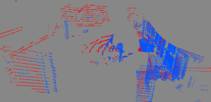
(a)

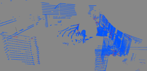
(b)

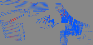
(c)

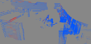
(d)

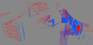
(e)

(f)

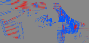
(g)

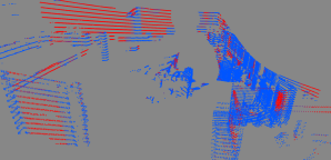
(h)

Figure 6: Joint point clouds colored by per-point quality $q_{k}$ ranging from blue (aligned) to red (misaligned). The location of the point cloud origin is highlighted in Fig. 9. Columns depict the same parameters for aligned (top) and misaligned (bottom) point clouds. (a,e): A fixed radius $r=0.3$ m gives a low $Q_{s}$ ratio from Eq. 7 $(Q_{s}=1.46)$, which makes it harder to learn a threshold to reliably separate aligned and misaligned point clouds. (b,f): Dynamically adjusted radius $r_{min}=0.3$ m,$\alpha=1.33,r_{max}=0.7$ m gives $(Q_{s}=2.93)$. (c,g): $\epsilon=10^{-8}$ is added $(Q_{s}=4.06)$. (d,h): $E_{\mathrm{reject}}=10\%$ is added. Then $Q_{s}=4.3$, and the point clouds are clearly separable.

We propose three optional strategies to address the ill-conditioned covariances due to variations in sampling density originating from the sensor. Option (1) is specifically intended to address the characteristic ring pattern that produces variations in sparsity. Option (2) that uses a dynamic radius can benefit both spinning lidar or radar where sparsity increase with range. Option (3) is intended mainly for 3d point clouds.

(1): Eq. 1 is modified to $h_{i}(\mathbb{p}_{k})=\frac{1}{2}\ln(2\pi e\det(\mathbb{\Sigma(p}_{k}))+\epsilon)$ where $\epsilon$ limits the lowest possible entropy. This makes sure that entropy is similar for points distributed along a line and a plane. The improvement can be seen by comparing the first and second column in Fig. 6.

(2): A dynamic radius enables the quality measure to include more points far from the sensor and correctly detect alignment and misalignment at large distances as depicted in the third column of Fig. 6 (c & g). Radius $r$ is chosen based on the distance $d$ between the point $\mathbb{p}_{k}$ and the sensor location to account for that point density decrease over distance. The radius is hence selected as: $r=d\sin(\alpha)$ in the range $r_{min}<r<r_{max}$ where $\alpha$ is the vertical resolution of the sensor provided by the data-sheet. For other sensor types e.g. RGB-D, the resolution could be chosen similarly according to the angular sensing resolution.

(3): Remove $E_{\mathrm{reject}}$ percent of points $\mathbb{p}_{k}$ with the lowest entropies. The effect is depicted in the rightmost column of Fig. 6.

III-D CorAl for spinning radar

Given the presented CorAl approach, this section describes the additional steps used to enable CorAl to operate on spinning radar data. It contains a short introduction to the format of spinning radar data and proposes a novel feature extraction method that produces a high-quality point cloud from radar data.

Spinning FMCW radar produces $360^{\circ}$ sweeps on polar coordinates seen in Fig. 7. The raw data is represented as a matrix ($Z_{N_{a}\times N_{r}}$).

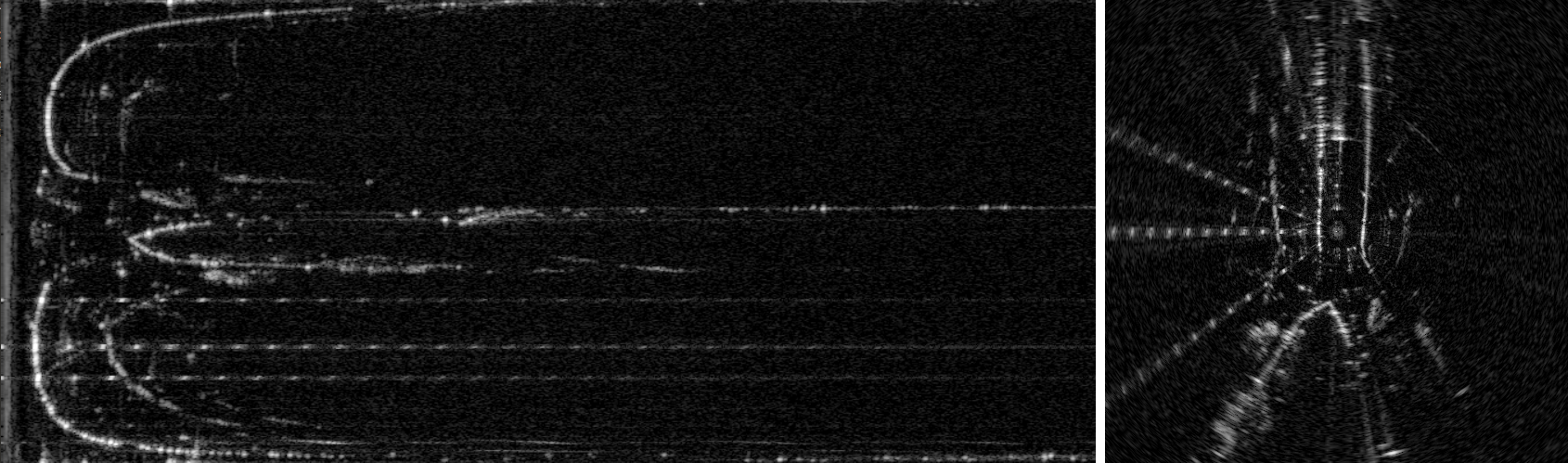
Figure 7: Polar and Cartesian spinning radar data.

The radar outputs $N_{r}$ range bins (the number of columns in Fig. 7), given the max range $R$, the range resolution is $\gamma=R/N_{r}$. Likewise, the radar provides $N_{a}$ azimuth bins (rows in Fig. 7). Each pixel $(a,r)$ with $a\in\{1..N_{a}\},r\in\{1..N_{r}\}$ holds the reflected intensity and can be converted into Cartesian space as

$$\mathbf{p}=\begin{bmatrix}p_{x}\\ p_{y}\end{bmatrix}=\begin{bmatrix}r\gamma\text{cos}\left(\theta\right)\\ r\gamma\text{sin}\left(\theta\right)\end{bmatrix},$$ (8)

where $\gamma$ is the range resolution of the radar and the azimuth angle $\theta$ can be computed via $\theta=2\pi a/N_{a}$.

III-E Computation of Radar Intensity Peak (RIP)-features

From raw radar data as seen in Fig. 7, the goal is to produce accurate point clouds suitable for alignment classification. We build on top of the radar filter “$k$-strongest” [1] that efficiently computes a mask that removes noise and keeps significant features that are useful for odometry estimation. Over all the $1..N_{r}$ range bins, the $k$ highest intensity bins that additionally exceed the expected noise level $z_{min}$ are selected. The noise level $z_{min}$ mitigates speckle noise and uncertain or false detections in absence of real obstacles. The limitation of $k$ returns per azimuth complements $z_{min}$ by mitigating multi-path reflections and receiver saturation under the assumption that true landmarks have higher intensity.

This method efficiently provides a mask in regions around true landmarks and generalizes well across environment types (the same $k$ and $z_{min}$ values work well in our odometry pipeline [1] for the road as well as underground applications). However, it does not accurately reconstruct landmark surface locations. We tested this representation and found that the method is unsuitable for detecting small misalignments. For that reason, we propose an additional step aiming to further analyze masked regions and compute stable features located on Radar Intensity Peaks (RIP)-features. We aim to efficiently and accurately detect surface locations by finding peaks within masked regions where intensity is consistently high over a local neighbourhood. To do so, we combine non-maximum-suppression on the 1D intensity-range signals together with a region strength criterion. Azimuths bins are analyzed independently without considering neighboring azimuth bin. For each range bin within the masked radar image, and neighboring range bins outside the masked region, the region strength is computed as the average intensity within a window (with size $w$) of neighboring range bins. Second, we select all range bins where region strength exceeds neighboring bins with the additional criteria that region strength must exceed the expected region noise floor. The algorithm is formally described in Alg. 1. Typical behavior is depicted in Fig. 8. Structures such as buildings and vehicles appear with higher intensity and give rise to the most stable features; these are good candidates for detecting misalignment as surface location uncertainty is low. When there are secondary landmarks within a single beam observed with intensity, e.g. a bush in front of a building, these give rise to features more scarcely. Moving vehicles have little impact on the CorAl score if driving sufficiently fast, i.e. for a radar spinning at $4$ Hz, vehicles moving faster than $14.4$ km/h will be outside the CorAl radius ($r=1$ m) boundary within consecutive observations, and will not contribute to misalignment.

Figure 8: Sparse radar filtering presented in Cartesian space using the RIP (Radar Intensity Peaks) features proposed in Sec. III-E. The raw radar data (black-yellow) is first masked using “$k$-strongest” (cyan) to find areas that contain landmarks. Stable RIP-features (black dots) are then computed accurately around intensity peaks.

Algorithm 1 RIP-Feature extraction

Input: $Z_{N_{a}\times N_{r}}$ Polar radar image
Parameters: window size $w$, masked points per azimuth $k$, noise filter $z_{min}$
Output: $\mathcal{F}_{rip}=\{(r,a)_{i}\}$ set of range and angle tuples

1:$\mathcal{F}_{rip}\leftarrow\emptyset$

2:for $a\leftarrow 1..N_{a}$  do //all azimuth bins

3:     $\mathcal{K}\leftarrow kstrongest(\>Z(a,1..N_{r}),\>k,\>z_{min})$

4:     Initialize table S //Scores

5:     for $r\in\mathcal{K}\cup neighbors(\mathcal{K},w)$ do

6:         $Scores[r]=1/(2w+1)\sum_{n=r-2}^{r+2}=Z(a,n)$      

7:     for $r\in\mathcal{K}$ do //only search masked points

8:         if $\textbf{S}[r]>=max(\>neighbors(r,w)\>)$  then

9:              if $\textbf{S}[r]>z_{min}$  then

10:                  $\mathcal{F}_{rip}\leftarrow\mathcal{F}_{rip}\cup\{(r,a)\}$                             

III-F Self-supervised learning of alignment classification

We learn alignment classification based on our quality measure in a self-supervised fashion from an accurate sensor pose signal. In this paper, we use either an external ground truth system or a lidar/radar odometry estimator. For each pair of scans, we compute the quality measure 1) directly and 2) after inducing a (sensor frame) offset in position and orientation on the later scan location. This allows the system to produce positive (aligned) and negative (misaligned) data points for training and to learn classification boundaries according to the magnitude of induced errors. To avoid over-fitting and to produce valuable insight into the alignment class separability based on the evaluated score functions, we use a simple logistic regression as a model for classification:

$$\begin{split}&p=\frac{1}{1+e^{-z}},\\ &z=\beta_{0}+\beta_{1}x_{1}+\beta_{2}x_{2},\\ \end{split}$$ (9)

$$y_{pred}=\begin{cases}\mathrm{aligned}&\mathrm{if}\>p\geq t_{h}\\ \mathrm{misaligned}&\mathrm{if}\>p<t_{h},\end{cases}$$ (10)

where $p$ is the class probability and $x_{1},x_{2}$ are input variables to which we pass quality measures. For the CorAl quality presented here, we refrain from passing the one variable quality measure $Q=H_{joint}-H_{sep}$ and instead pass the joint and separate entropies as: $x_{1}=H_{joint},x_{2}=H_{sep}$. This allows the model to learn the mapping from $H_{sep}$ and $H_{joint}$ to alignment probability $p$ implicitly.

The model parameters in Eq. LABEL:eq:class-pz ($\beta_{0}$, $\beta_{1}$, $\beta_{2}$) are learned during training. The classification probability threshold $t_{h}$ can be adjusted after training has been carried out in order to balance sensitivity to false-positive rate. Increasing the threshold will cause fewer well-aligned pairs to be correctly classified as aligned (decrease recall), but will reduce the rate of misaligned pairs being falsely be classified as aligned (increase precision). In our experiments we used the default threshold $t_{h}=0.5$. During training, weights of data points were adjusted inversely proportional to class occurrence to mitigate bias.

‘

IV Evaluation on lidar data

In this section, we present a quantitative evaluation of alignment quality classification with CorAl for 3D lidar data. An evaluation for 2D radar data will follow in Sec. V.

In order to compare the method presented in this paper to previous work related to 3D point cloud alignment assessment, we follow the procedure of evaluation as carried out in [12]. For the results in this section, we use an equal portion of aligned and misaligned point clouds, where misaligned point clouds are created by adding an offset for each point cloud pair: an angular offset ($e_{\theta}=0.57^{\circ}=0.1$ rad) around the sensor’s vertical axis and a random translation $(x,y)$ offset at a distance ($e_{d}=0.1$ m) from the ground truth. These errors are large enough to be meaningful to detect in various environments, yet challenging to classify.

IV-1 Evaluated lidar methods

The evaluated methods; MME, CorAL, CorAl-median, NDT, Rel-NDT and FuzzyQA are briefly summarized here together with their most important parameters. For CorAl, FuzzyQA and Rel-NDT, two values (that represent the quality measure) are passed to $x_{1}$ and $x_{2}$, for MME and NDT, a single value is passed to $x_{1}$ while $x_{2}$ is set to zero. To make a fair comparison, we use a similar radius for NDT, MME and CorAl.

MME

Mean Map Entropy (MME) as proposed by Droeschel and Behnke [47]. The quality measure corresponds to $H_{joint}$ from Eq. 3. The parameter is the same radius $r$ used for computing the per-point differential entropy. The MME is passed to the classifier as: $x_{1}=H_{joint},x_{2}=0$.

CorAl

as described in Secs. III-B and III-C and in [17]. Parameters are $r_{\mathrm{min}}$, $r_{\mathrm{max}}$ and $\alpha$ to determine nearby points radius, and $E_{\mathrm{reject}}$ to set outlier rejection ratio and $\epsilon$ for mitigating ill-conditioned entropies. The joint and separate entropy are passed separately to the classifier: $x_{1}=H_{joint},x_{2}=H_{sep}$, an intuition is presented in  III-F.

CorAl-Median

$H_{s},H_{j}$ are modified to calculate the median entropy rather than the mean entropy, we hypothesize that this modification can be more robust to outliers. Except for modification, we used the same parameter and methodology described in the previous paragraph.

NDT (point-to-distribution normal-distributions transform)

The NDT quality describes the likelihood of finding the points in $\mathcal{P}_{b}$, given the NDT representation of $\mathcal{P}_{a}$. The method uses the 3D-NDT [48] representation, which constructs a voxel grid over one point cloud, and computes a Gaussian based on the points in each voxel. The likelihood of finding the points in $\mathcal{P}_{b}$ is computed as

$$s=\frac{\sum_{k=1}^{n}\tilde{p}(\mathbf{p}_{k})}{n},$$ (11)

where $n$ is the number of overlapping points, defined as those points that fall in an occupied NDT voxel, or in a voxel that is a direct neighbor of an occupied voxel, and $\tilde{p}$ is the probability density function associated with the nearest overlapping NDT-cell. This is similar to the “NDT3” variant in [12]. The most important parameter for NDT is the voxel size $v$ which is set equal to $2*r$ in our evaluation, as this makes the volumes used for the sample covariance of NDT cells and the entropy in CorAl comparable. The NDT quality $s$ is passed as: $x_{1}=s$.

Rel-NDT

as described in [17]. This variant aims to improve the re-utilization of learned NDT classification parameters when applied to new environments. The idea (similar to CorAl) is that environment type is reflected in the average entropy of the scene and can be combined with the NDT score to improve the classification. Similar to the MME, we compute the average differential entropy. However, instead of recomputing the sample covariances around each point $p_{k}$, we use the covariances directly from the NDT representation of $\mathcal{P}_{a}$. This is only done in overlapping regions and no additional parameter to NDT is required. The NDT score $s$ and the overlapping NDT differential entropy (NDT-entropy) is passed as: $x_{1}=s,x_{2}=NDT-entropy$

FuzzyQA

FuzzyQA [14] measures the alignment quality by a ratio $\rho=\frac{\mathrm{AFCCD}}{\mathrm{AFPCD}}$, where AFCCD and AFPCD are two indexes describing the points’ disposition and dispersion around fuzzy cluster centers. In [14], two point clouds are considered to be coarsely aligned if $\rho<1$. In this paper, we pass AFCCD and AFPCD separately to the classifier input $x_{1}=AFCCD,x_{2}=AFPCD$ in order to learn a generalizable separator.

IV-A Qualitative evaluation, live robot data

First, we present qualitative results from real-world data in a warehouse environment. A forklift equipped with a Velodyne HDL-32E 3D laser scanner was manually driven at fast walking speed in the warehouse depicted in Fig. 9. The environment covered in this data set varies from large and open areas with walls in line of sight to small and narrow aisles between shelf racks.

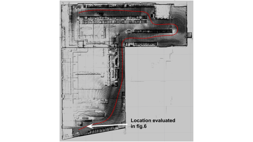
Figure 9: Data acquired by a truck in a warehouse environment. The sensor trajectory is drawn in red. The environment in the figure is 50 m $\times$ 50 m and the sequence length is 102 m. In the first segment of the trajectory, starting at the bottom left, the walls are clearly visible. The final segment is located between aisles where walls are typically out of sight and the sensor observes more complex structures such as shelves. The truck has worn out slightly oval wheels which introduces a large degree of vibrations, hence alignment quality is expected to be low.

To generate ground-truth alignments for the warehouse dataset, we first aligned the point clouds using a scan-to-map approach [8]. We have then inspected the alignment between subsequent scans and found that at least 40/484 (8.3%) point clouds were impaired by rigid misalignments or non-rigid distortions from vibrations and motion to the extent that these could be visually located. Alignment classification was then performed on the remaining scans by inducing errors as described in sec. IV. We used the following parameters as they provided a relatively high value of $Q_{s}$ for the first scan pair in the dataset: $\alpha=0.92^{\circ}$, $E_{\mathrm{reject}}=0.2$, $r_{min}=0.2$ m, $r_{max}=1.0$ m and voxel size $v=2r_{min}=0.4$ m. We found that CorAl-mean, MME and NDT reached an accuracy of $96\%$, $70\%$ and $99\%$ respectively. In this case, NDT performs slightly better than CorAl. We believe that the relatively lower result is due to the experimental setup. CorAl is highly sensitive to low quality in training data. In this case, even after removing the worst data points in the ground truth set, the level of vibrations from the worn-out wheels remain high in a large number of data points used for training and evaluation. This makes it challenging to learn the detection of small errors using the CorAl quality measure. Whether this is high sensitivity is the desired behavior depends on the application.

IV-B Quantitative evaluation, ETH benchmark data set

Our main quantitative evaluation of CorAl’s performance on 3D lidar point clouds is done by using the public ETH registration dataset [49]. It contains several sequences representing a wide variety of environments, which will serve us to evaluate how well CorAl generalizes across different kinds of them. Specifically, this dataset includes 3 sequences in structured environments (Apartments, ETH Hauptgebaude, Stairs), 3 sequences in semi-structured environments (Gazebo in summer, Gazebo in winter, Mountain plain) and 2 challenging sequences in unstructured environments (Wood in summer, Wood in autumn). In Figs. 10, 12 and 11, the training results for structured environments are shown in blue, the ones for semi-structured environments in brown, and the ones for unstructured environments in green. Each sequence contains between 31 and 47 scans acquired from stationary positions. The dataset contains accurate ground truth positions, required to evaluate the different methods. In order to make the evaluation fairer, more realistic, and applicable to real applications, we downsampled the original dense point clouds using a voxel grid of 0.08 m. In all the training experiments, CorAl has been run on an Intel Core i7-7820X desktop CPU, achieving an overall run-time of $0.246\pm 0.095$ seconds per point cloud pair. Also, since this dataset has less variation in sampling density compared to the warehouse one employed in Sec. IV-A, we used a fixed radius $r=0.3$ m and set $E_{\mathrm{reject}}=20\%$ and $\epsilon=0$. Finally, the NDT voxel size was set equal to two times the CorAl radius, i.e, $v=2r=0.6$ m. This way, the diameter of influence for CorAl and the width of NDT cells are similar.

In these conditions, we carried out three different kinds of training, which are aimed at showing how the proposed CorAl method can achieve generalization. Training has been performed with increasing difficulty, as explained below.

IV-B1 Separate training

First, we evaluate the capability to learn classification in a specific type of environment. The classifiers were trained and evaluated on each sequence separately, using 5-fold cross-validation. This evaluation serves as a reference for the cross-environment evaluations below. Results are shown in Fig. 10.

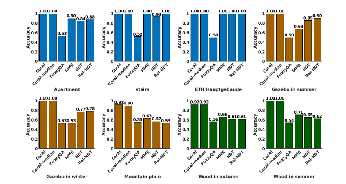
Figure 10: Separate training. The overall accuracy was CorAl: $98\%$, CorAl-median: $98\%$ FuzzyQA: $53\%$ MME: $77\%$ NDT: $78\%$ Rel-NDT: $80\%$

We found that all methods except FuzzyQA performed well in structured environments. For instance, MME scored around 90–100%, which clearly indicates that even a method that is highly influenced by the environment can successfully assess alignment quality if the environment is structured and not changing substantially. In contrast, we did not expect that FuzzyQA would achieve a good classification performance since it is specifically designed to classify coarse alignment.

In the semi-structured and unstructured sequences, only CorAl and CorAl-median performed well, with consistently $>$90% accuracy, even in the most challenging sequences. All other methods are only slightly better than random, except for the gazebo sequences. Rel-NDT slightly outperforms NDT, however not consistently. Both NDT methods performed decently (77–90%) in the gazebo sequence, but poorly in the unstructured Wood sequences (60–65%), indicating that NDT requires at least some structure or surfaces free from foliage to be effective as an alignment correctness measure.

IV-B2 Joint training

The second test evaluates how the methods are able to learn alignment classification when trained in a variety of environments. To do that, the methods need to be versatile. The training was performed on all the ETH sequences together, and evaluation was then done on each sequence individually. The results are shown in Fig. 11.

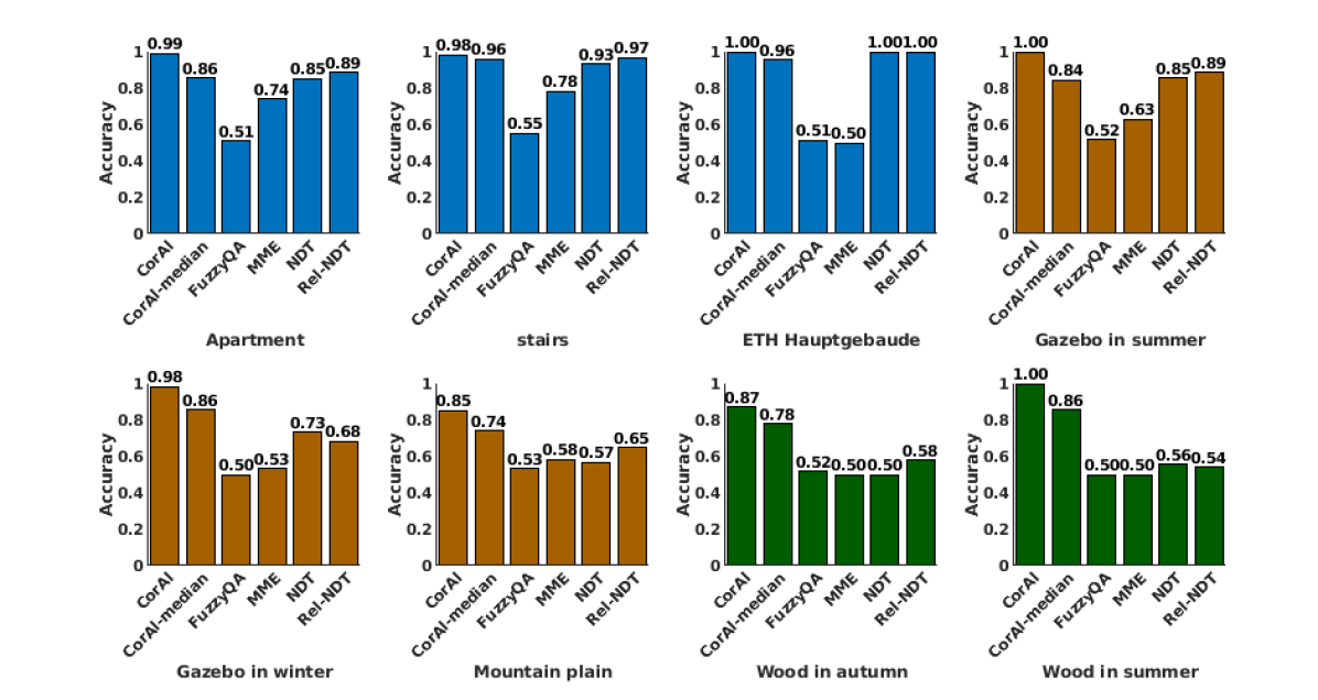
Figure 11: Joint training. Overall accuracy CorAl: $96\%$, Coral-median: $95\%$ FuzzyQA: $52\%$ MME: $60\%$ NDT: $75\%$ Rel-NDT: $78\%$

As can be expected, the accuracy of all classifiers decreased compared to the previous test. CorAl still performs best, with an accuracy of 85–100% in all cases. CorAl-median reached a slightly lower accuracy compared to CorAl. Rel-NDT performed better than NDT in most cases, however not consistently. The generally high accuracy of CorAl indicates that it is possible to find general parameters that make the method valid in a range of substantially different environments.

IV-B3 Generalization to unseen environments

The final test evaluates how classifiers perform in environments with different characteristics than those observed in the training set. We trained and evaluated different sequences and environments. The 3 structured environments were used for training and the remaining 5 (semi-structured and unstructured) were used for evaluation and vice versa. The classification accuracy is depicted in Fig. 12.

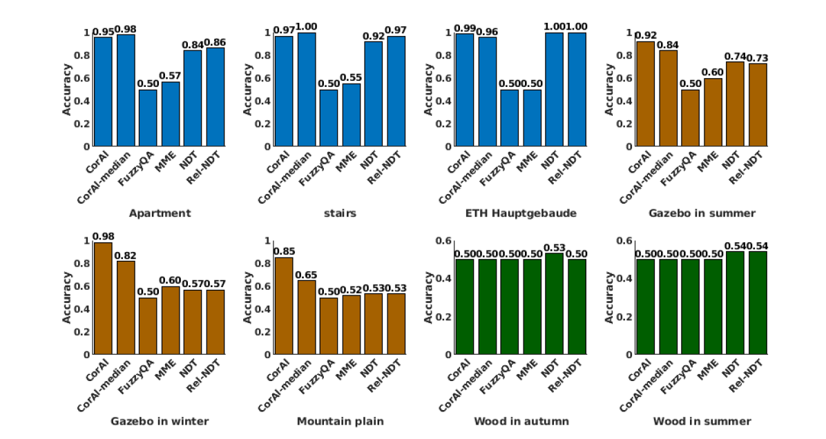
Figure 12: Evaluation on unseen environments. Overall accuracy: $83\%$, CorAl-median: $79\%$ FuzzyQA: $50\%$ MME: $54\%$ NDT: $72\%$ Rel-NDT: $72\%$, In structured and semi-structured environments: $95\%$, Coral-median: $88\%$ FuzzyQA: $50\%$ MME: $56\%$ NDT: $78\%$ Rel-NDT: $79\%$.

When trained on structured and evaluated on semi-structured environments, CorAl performed accurately (85–98%) and other methods performed close to random except NDT for Gazebo summer ($74\%$). No method generalized well when training on structured data and evaluated on unstructured environments. On the other hand, learning from semi-structured and unstructured environments was enough to afford very high accuracy in structured environments with CorAl – very close to what was attained with joint training on all sequences. The previous joint evaluation shows that it is possible to train a model that is simultaneously accurate in all environment types. Hence, we believe that the reason the classifier trained in a structured environment does not generalize to an unstructured environment is that the model overfits when not trained with sufficiently diverse and challenging data.

V Evaluation of large-scale radar data

In this section, we present a thorough evaluation of the problem of alignment correctness classification using data acquired by different spinning radars. In these experiments, we have employed both CTS350-X and CIR2014-H models by Navtech. We highlight multiple challenges in alignment correctness classification of radar data and consider the impact of practical challenges such as variation of parameters, distance between scans, and error magnitudes. Similar to the generalization training carried out in Sec. IV-B, we again use datasets with different characteristics for training and testing in order to understand how CorAl generalizes across different environment types. We compare our method to recently published radar-specific baselines (Sec. V-A).

Currently, there exist four public datasets for spinning radar localization research: Boreas, Radiate [50], Mulran [51] and the most established Oxford Radar RobotCar dataset [52]. We selected Oxford (Fig. 14) and Mulran (Fig. 15) which both have accurate ground truth positioning and similar sensor range resolution ($0.0432$ m and $0.0595$ m respectively). Additionally, MulRan contains a diverse variety of surrounding environment types including urban, mountain, and fields which allows us to test how the methods generalize outside of urban environments. In Sec. V-E we used the sequence “10-12-32” from Oxford and “KAIST02” from Mulran. In all other experiments, each data point and deviation is computed over the sequences 10-12-32, 18-14-14, 18-14-46 and 18-15-20 from the Oxford dataset. Both datasets contain a variety of weather conditions and traffic from vehicles, pedestrians and bikers. Hence these sequences constitute realistic urban scenarios.

To make the method evaluation more realistic for urban applications, we generate 4 misalignments symmetrically around each aligned data-point: two in the longitudinal directions of the driving direction (forward and backward) where localization uncertainty due to motion and landmarks is generally higher, and two in the lateral direction (left and right) with lower uncertainty. Training weights and evaluation metrics are balanced accordingly.

Depending on the application and sensor, various error levels can be of interest. E.g. odometry is expected to be more accurate compared to loop closure and relocalization and requires detection of smaller errors. We produced the position error distribution of the currently most accurate method for radar odometry estimation CFEAR, the distribution is depicted in Fig. 13. The $0.995$ quantile corresponds to a longitudinal and lateral error of $0.29$ m and $0.12$ m, respectively. Detecting errors above this point $(>~{}0.29)$ m would be meaningful for the task of odometry. These are larger error levels compared to what we considered in our previous evaluation on lidar ($0.1$ m) in Sec. IV. Using the same step size between error levels as in [12], we define small, medium and large errors as $0.3$ m, $0.5$ m and $0.7$ m respectively. These errors are higher than the ones defined for lidar sensors, which is necessary as localization uncertainty is expected to be higher, e.g. due to the larger scale, higher motion and low spinning rate of radar used in our experiments. For a vehicle moving at 50 km/h with a radar spinning at 4 Hz, the motion distortion from translation only is 3.5 m between the first and last segment of a scan unless carefully compensated for.

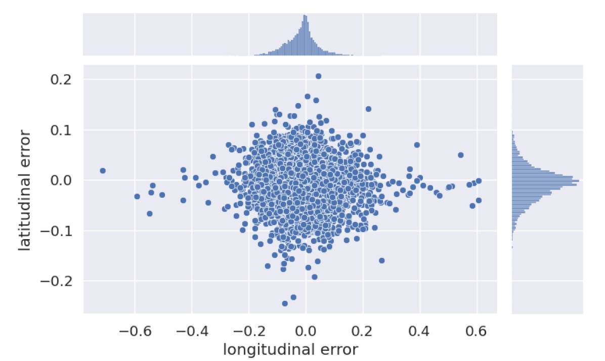
Figure 13: Investigation of error distribution in radar odometry.

Figure 14: Locations traversed in the urban Oxford dataset.

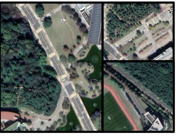
Figure 15: Examples of semi-structured regions in the MulRan dataset.

V-A Evaluated radar methods

Here we give a brief introduction of all compared methods for feature extraction, quality measure and parameters. In all cases, we have compensated for motion distortion effects as described in [1], and features within a minimum range of $2.5$ m are removed in order to discard false detections located on the experimental setup itself.

Cen2018

A method for extracting radar features and estimating ego-motion proposed by Cen and Newman [41]. We use their method for extracting features from intensity gradients and peaks with the improved configuration described by Burnett [38], where the probability threshold is increased to $z_{q}=3.0$ and a Gaussian filter is added with $\sigma=17$ as described in [38]. We do not carry out data association as described in the original publication but instead perform a radius search and compute the point-to-point quality measure with association radius $radius=3$ m. The sum of point-to-point distances is normalized by the number of points and passed to $x1$.

CFEAR

current state-of-the-art in Radar odometry estimation [1]. We use the CFEAR-feature extraction method, with the quality measures (P2P, P2L and P2D). Radar data is first filtered using $k$-strongest as described in Sec. III-E by first applying the $k$-strongest filter and then using a grid-based approach that estimates a set of oriented surface points for each grid cell that contains points. In our experiments, we used the same parameters as described in [1] except with minor changes to $z_{min}=60$ and $radius=3$ m for consistency with Cen2018. For this method, we extend the logistic regression model with a third input dimension $x_{3}$ to incorporate more available information. Specifically, the absolute score, the number of correspondences and the normalized score are passed to $x_{1},x_{2}$ and $x_{3}$ respectively.

CorAl-Radar (ours)

We set $r_{\mathrm{min}}=r_{\mathrm{max}}=1$, $E_{\mathrm{reject}}=0$ and $\epsilon=0$. CorAl-Radar extends the previous parameter CorAl set with window size $w=2$, $k=12$ and $z_{min}=70$ for computing RIP-features (Sec. III-E). The latter parameters ($k$ and $z_{min}$ have the same meaning as in the method CFEAR and are fixed in our experiments and equal for CFEAR and CorAl. The joint and separate entropy are passed separately to the classifier: $x_{1}=H_{joint},x_{2}=H_{sep}$ as described in Sec. III-F.

V-B Method and performance analysis

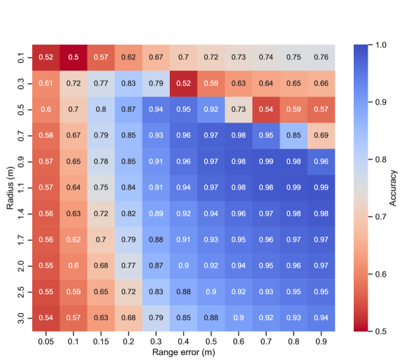
Figure 16: Heat map for the classification accuracy obtained by using the CorAl method, as a function of the translation error and the association radius employed. While the radius is optimally chosen slightly larger compared to the translation maximum error CorAl intends to detect, $r=1$ m provides good capabilities to detect errors larger than $0.2$ m.

We start our evaluation by studying the radius parameter. While a low radius is required to detect the smallest alignment errors, a too conservatively chosen radius will make larger errors more challenging to detect. This is because the computation of entropy is only sensitive to the displacement of points within the radius. Hence is the capability to detect errors with different magnitudes is related to the selection of radius as seen in Fig. 16. Generally, the radius should be chosen larger than the maximum error to detect. however as confirmed by our evaluation, detecting very large alignment errors $>1$ m is not a challenging task and CorAl can therefore be complemented with a quality metric such as point-to-point or point-to-line. We found that a radius set to $r=1$ m provides a good trade-off and allows the detection of fairly large errors.

The runtime performance of CorAl is shown in Tab. I. All timing statistics have been computed out on an Intel i7-11850H laptop CPU. All representations and quality metrics are efficient to compute ($<$5 ms single-threaded) except Cen2018 which runs at 14 ms with a multi-thread implementation.

Feature extraction Quality measure Method Mean [ms] Std. dev. ($\sigma$) Mean [ms] Std. dev. ($\sigma$) Threads CFEAR-P2P 3.93 0.10 0.69 0.04 single CFEAR-P2L 4.88 0.08 0.83 0.09 single CFEAR-P2D 3.92 0.08 0.75 0.05 single CEN2018-P2P 14.21 0.25 3.05 0.41 multiple CorAl (ours) 2.07 0.03 3.47 0.29 single

TABLE I: Computation time (milliseconds) for feature extraction and quality measure.

V-C Detecting errors with various magnitudes

We aim to investigate the extent to which errors of different magnitudes ranging from $0.05$ up to $0.9$ meters can be detected. The performance is quantified using accuracy and the area under the ROC curve (AUC). The obtained results are depicted in Fig. 17. In these plots, we report results for two classes of scans, with varying distances between scans: scans taken at least 0 m apart (consecutive scans) and scans taken at least 10 m apart. In general, these results show that the proposed CorAl method achieves the best classification accuracy and AUC in the evaluated range when the spacing between scans is low. Under these conditions, none of the other methods reach similar performance. The next-best method is CFEAR-P2L, which robustly detects large translation errors but only when they are greater than 0.7 meters. When scan spacing is large ($10$ m), CorAl is still the most accurate for small errors (less than 0.4 meters) although the accuracy achieved is not very high. A summary of these results can be found in Tab. II.

Orientation errors are evaluated separately as depicted in Fig. 18. Such errors are added here in the same way as in the case of evaluation on lidar data, i.e., by adding an angular offset $e_{\theta}$ around the sensor’s vertical axis. In general, the CFEAR and Cen2018 quality metrics demonstrate similar or improved performance compared to CorAl for orientation errors. We believe this is because orientation errors displace observations proportionally to the distance of observation. At large distances, the conservative data association of CorAl makes the metric less sensitive, unless combined with the optional parameter that dynamically increases radius accordingly.

Translation error Method Small (0.3 m) Medium (0.5 m) Large (0.7 m) CFEAR-P2P $0.59/0.61$ $0.69/0.77$ $0.85/0.95$ CFEAR-P2L $0.66/0.77$ $0.89/0.95$ $0.97/0.99$ CFEAR-P2D $0.57/0.66$ $0.76/0.85$ $0.89/0.96$ CEN2018-P2P $0.52/0.54$ $0.56/0.60$ $0.61/0.68$ CorAl (ours) $\mathbf{0.91}/\mathbf{0.98}$ $\mathbf{0.97}/\mathbf{1.00}$ $\mathbf{0.99}/\mathbf{1.00}$

TABLE II: Quality of classification results corresponding to each method used in this work, versus different translation errors. The values reported for each configuration are the mean accuracy and mean AUC, respectively, which also correspond to 0 meters of scan overlapping.

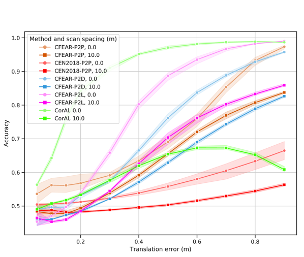
(a)

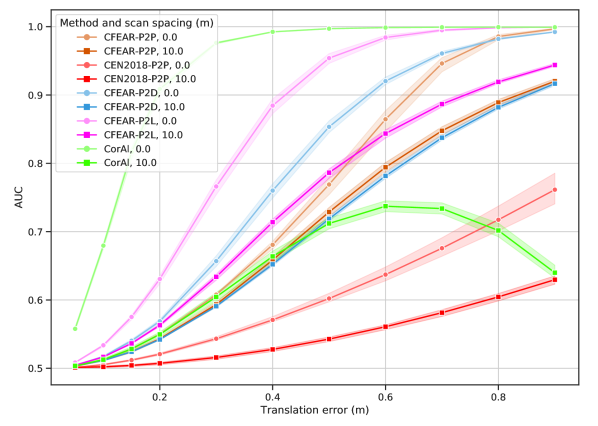
(b)

Figure 17: Accuracy and AUC vs translation error. (a) CorAl is the most accurate and can even detect small alignment errors of $0.3$ m with $>90\%$ accuracy when distance between scans is low. CFEAR-P2L requires $0.2$ m larger errors to reach similar level of accuracy. For large scan distances (less overlap), CFEAR-P2L is the most accurate with $~{}85\%$ accuracy. (b) CorAl generally achieves the best performance (well above $90\%$ even for small translation errors) when distance between scans is low. For large scan distances, CFEAR-P2L is the most robust method for any translation error.

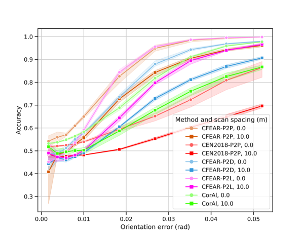
(a)

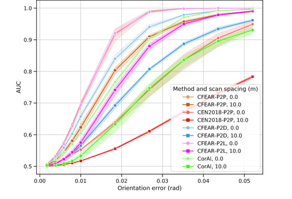
(b)

Figure 18: Classification accuracy vs orientation error. The radius parameter is set to $r=3$ m.

V-D Variation in distance between scans

We have also carried out another set of experiments aimed at analyzing the impact of scan spacing distance. In this case, we consider two different levels of translation errors (0.3 and 0.6 meters). Detecting small errors from scans separated by large distances is challenging due to dynamics changes, lower overlap, and because sensor characteristics make observed landmarks appear differently from different perspectives, a phenomenon previously discussed in the literature [2]. As expected, the results in Fig. 20 show that classification accuracy is reduced for all methods when scan spacing is increased. Despite this, CorAl was able to achieve $~{}87\%$ accuracy for $0.6$ m errors at $5$ m spacing. After $7$ m, CFEAR-P2L accuracy surpasses CorAl, which accuracy reduces more quickly We believe the worse performance for larger scan spacing depends on radar-specific challenges as depicted in Fig. 19. When spacing is large, walls appear different due to beam divergence. CorAl is more sensitive to small errors and hence not expected to perform well in this scenario.

(a)

(b)

Figure 19: Bottom (red) and top (blue) scans acquired with small (a) and large (b) separation in distance. When distance is high, scans incorrectly appear to be misaligned due to a high level of beam divergence in current radar sensors. The impact is higher when landmarks are observed from different angles, which occur more often when the distance between scans is large.

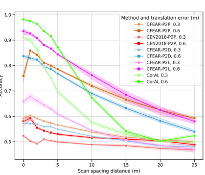
(a)

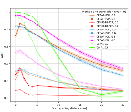
(b)

Figure 20: Accuracy and AUC vs scan spacing (overlap). Increasing distance between scans makes classification more challenging. CorAl is most accurate for small errors while CFEAR-P2L is more accurate when distance between scans is higher.

V-E Generalization across environments

Similarly to the evaluation of generalization capabilities for lidar data (Sec. IV-B3), we are interested in comparing how the proposed approach can classify the scans when the training and test data sequences are not from the same type of environment. We used the urban Oxford dataset (Fig. 14) and the partly semi-structured Mulran dataset (Fig. 15). The accuracy for Oxford and Mulran is depicted in Fig. 22. We make the same observation as in the lidar generalization experiments in Sec. IV-B; classification of a method trained from a semi-structured (more diverse) data set will generalize better.

To train with the structured data (Oxford) and testing on the semi-structured data (Mulran) the accuracy obtained is 91% compared with 96% if the testing and training data is switched. If the datasets are considered fully separately the accuracy for Oxford and Mulran is 97.9% and 95.7% respectively. ROC curves are provided in Fig. 21, which also illustrates the generalization capabilities.

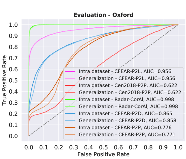
(a)

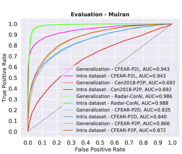
(b)

Figure 21: Comparison where methods are trained and tested on the same (Intra dataset) and separate (Generalization) datasets with varied discrimination treshold. We found that CorAl is the most accurate in both environments regardless of where the method is trained. For our proposed method, the best level of generalization is achieved when training on the semi-structured dataset MulRan and testing on the structured Urban Oxford dataset.

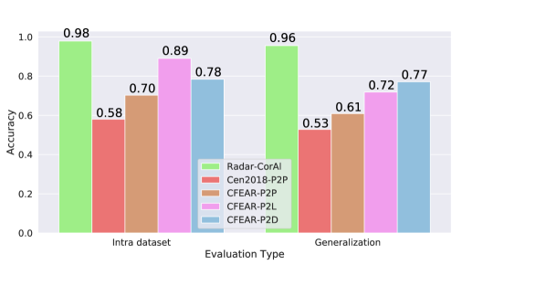
(a)

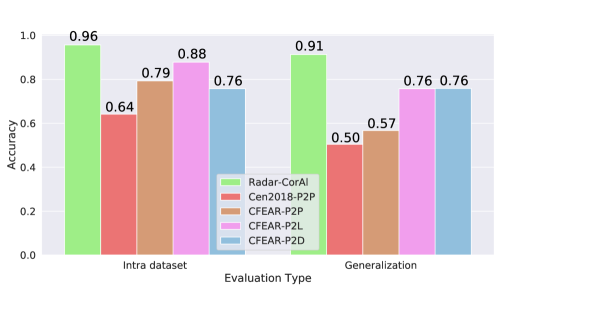
(b)

Figure 22: Classification accuracy of small errors ($0.5$ m) for a fixed discrimination threshold ($t_{h}=0.5$) when training and evaluating on the same dataset (intra dataset) and when training and evaluating on different datasets (generalization).

VI Conclusions

In this paper, we presented CorAl, a principled and intuitive quality measure and self-supervised system that learns to detect small alignment errors between pairs of previously aligned point clouds. CorAl uses dual entropy measurements found in the separate point and in the joint point cloud to obtain a quality measure that substantially outperforms previous methods on the task of detecting small alignment errors within a benchmarking lidar dataset, and within a large-scale urban dataset for spinning radar.

In this work, we proposed a two-step filtering strategy that operates on challenging radar data and produces a high-quality point cloud. By combining our filtering method with CorAl we were able to detect small alignment errors in urban settings using only a spinning radar. We found the method to be accurate in a wide range of environments and can generalize to new unseen environments without retraining. Using a roof-mounted radar within realistic trafficked urban scenarios, we achieve up to $98\%$ accuracy in detection of $0.5$ m errors when trained in the same environment, and up to $96\%$ accuracy when trained on another environment type. Our experiments on both lidar and radar data demonstrate that CorAl achieves a high level of generalization between structured and semi-structured environments. We also found that learning from more challenging less structured environments results is advantageous for generalization. In our lidar experiments, we even found that CorAl was able to generalize from unstructured (woods) to structured indoor environments. However, none of the evaluated methods generalized well when trained in structured environments only and evaluated in an unstructured environment, and this remains a challenging problem.

We believe that the presented system has great potential to serve as an alignment quality tool for point clouds and can improve localization robustness by equipping odometry, relocalization, and loop closure systems with the capability of introspectively detecting small errors in diverse environments.

References

- [1] D. Adolfsson, M. Magnusson, A. Alhashimi, A. J. Lilienthal, and H. Andreasson, “CFEAR radarodometry - conservative filtering for efficient and accurate radar odometry,” in 2021 IEEE/RSJ International Conference on Intelligent Robots and Systems (IROS), 2021, pp. 5462–5469.
- [2] D. Adolfsson, S. Lowry, M. Magnusson, A. Lilienthal, and H. Andreasson, “A Submap per Perspective - Selecting Subsets for SuPer Mapping that Afford Superior Localization Quality,” in 2019 European Conference on Mobile Robots (ECMR), Sept. 2019, pp. 1–7.
- [3] B. Della Corte, H. Andreasson, T. Stoyanov, and G. Grisetti, “Unified Motion-Based Calibration of Mobile Multi-Sensor Platforms With Time Delay Estimation,” IEEE Robotics and Automation Letters, vol. 4, no. 2, pp. 902–909, Apr. 2019.
- [4] A. C. M. Tavares, F. J. Lawin, and P. Forssén, “Assessing losses for point set registration,” IEEE Robotics and Automation Letters, vol. 5, no. 2, pp. 3360–3367, 2020.
- [5] J. Zhang and S. Singh, “LOAM: Lidar odometry and mapping in real-time,” in Robotics: Science and Systems, 2014.
- [6] J. Tang, L. Ericson, J. Folkesson, and P. Jensfelt, “Gcnv2: Efficient correspondence prediction for real-time slam,” IEEE Robotics and Automation Letters, vol. 4, no. 4, pp. 3505–3512, 2019.
- [7] S. Nobili, G. Tinchev, and M. Fallon, “Predicting alignment risk to prevent localization failure,” in 2018 IEEE International Conference on Robotics and Automation (ICRA), 2018, pp. 1003–1010.
- [8] H. Andreasson, D. Adolfsson, T. Stoyanov, M. Magnusson, and A. J. Lilienthal, “Incorporating ego-motion uncertainty estimates in range data registration,” in 2017 (IROS), Sep. 2017, pp. 1389–1395.
- [9] Y. Chen and G. Medioni, “Object modeling by registration of multiple range images,” in Proceedings. 1991 IEEE International Conference on Robotics and Automation, 1991, pp. 2724–2729 vol.3.
- [10] S. M. Rusinkiewicz, “Efficient variants of the ICP algorithm,” in The Third International Conference on 3D Digital Imaging and Modeling, 2001, pp. 145–152.
- [11] M. Magnusson, “The three-dimensional normal-distributions transform — an efficient representation for registration, surface analysis, and loop detection,” Ph.D. dissertation, Örebro University, Dec. 2009, Örebro Studies in Technology 36.
- [12] H. Almqvist, M. Magnusson, T. P. Kucner, and A. J. Lilienthal, “Learning to detect misaligned point clouds,” Journal of Field Robotics, vol. 35, no. 5, pp. 662–677, 2018.
- [13] T. Stoyanov, M. Magnusson, H. Andreasson, and A. J. Lilienthal, “Fast and accurate scan registration through minimization of the distance between compact 3D NDT representations,” The International Journal of Robotics Research, vol. 31, no. 12, pp. 1377–1393, 2012.
- [14] Q. Liao, D. Sun, and H. Andreasson, “Point set registration for 3d range scans using fuzzy cluster-based metric and efficient global optimization,” IEEE Transactions on Pattern Analysis and Machine Intelligence, vol. 43, no. 9, pp. 3229–3246, 2021.
- [15] D. Droeschel and S. Behnke, “Local multi-resolution representation for 6d motion estimation and mapping with a continuously rotating 3d laser scanner,” in In Proc. of IEEE Int. Conf. on Robotics and Automation (ICRA, 2014.
- [16] D. Barnes, R. Weston, and I. Posner, “Masking by moving: Learning distraction-free radar odometry from pose information,” in CoRL, ser. CoRL, L. P. Kaelbling, D. Kragic, and K. Sugiura, Eds., vol. 100. PMLR, 30 Oct–01 Nov 2020, pp. 303–316.
- [17] D. Adolfsson, M. Magnusson, Q. Liao, A. J. Lilienthal, and H. Andreasson, “CorAl – are the point clouds correctly aligned?” in European Conference on Mobile Robots (ECMR).
- [18] P. J. Besl and N. D. McKay, “A method for registration of 3-d shapes,” IEEE TPAMI, vol. 14, no. 2, pp. 239–256, Feb 1992.
- [19] L. Silva, O. R. Bellon, and K. L. Boyer, “Precision range image registration using a robust surface interpenetration measure and enhanced genetic algorithms,” TPAMI, vol. 27, no. 5, pp. 762–776, May 2005.
- [20] A. Segal, D. Haehnel, and S. Thrun, “Generalized-ICP,” in Robotics: Science and Systems V. Robotics: Science and Systems Foundation, jun 2009. [Online]. Available: https://doi.org/10.15607%2Frss.2009.v.021
- [21] H. Yin, L. Tang, X. Ding, Y. Wang, and R. Xiong, “A failure detection method for 3d lidar based localization,” in 2019 Chinese Automation Congress (CAC), 2019, pp. 4559–4563.
- [22] A. Makadia, A. Patterson, and K. Daniilidis, “Fully automatic registration of 3d point clouds,” 2006 IEEE Computer Society Conference on Computer Vision and Pattern Recognition (CVPR’06), vol. 1, pp. 1297–1304, 2006.
- [23] N. Akai, L. Y. Moralesl, and H. Murase, “Reliability estimation of vehicle localization result,” in 2018 IEEE Intelligent Vehicles Symposium (IV), 2018, pp. 740–747.
- [24] R. Aldera, D. D. Martini, M. Gadd, and P. Newman, “What could go wrong? introspective radar odometry in challenging environments,” in 2019 IEEE Intelligent Transportation Systems Conference (ITSC), 2019, pp. 2835–2842.
- [25] P. Sundvall and P. Jensfelt, “Fault detection for mobile robots using redundant positioning systems,” in Proceedings 2006 IEEE International Conference on Robotics and Automation, 2006. ICRA 2006., 2006, pp. 3781–3786.
- [26] D. Landry, F. Pomerleau, and P. Giguère, “CELLO-3D: Estimating the covariance of ICP in the real world,” in IEEE (ICRA), May 2019, pp. 8190–8196.
- [27] O. Bengtsson and A.-J. Baerveldt, “Robot localization based on scan-matching—estimating the covariance matrix for the IDC algorithm,” Robotics and Autonomous Systems, vol. 44, no. 1, pp. 29–40, 2003.
- [28] J. Nieto, T. Bailey, and E. Nebot, “Scan-SLAM: Combining EKF-SLAM and scan correlation,” in Field and Service Robotics, ser. Springer Tracts in Advanced Robotics, P. Corke and S. Sukkariah, Eds. Springer, 2006, pp. 167–178.
- [29] S. M. Prakhya, L. Bingbing, Y. Rui, and W. Lin, “A closed-form estimate of 3d ICP covariance,” in 2015 14th IAPR (MVA), 2015, pp. 526–529.
- [30] A. Censi, “An accurate closed-form estimate of ICP’s covariance,” in Proceedings of the IEEE International Conference on Robotics and Automation (ICRA), apr 2007, pp. 3167–3172.
- [31] E. B. Olson, “Real-time correlative scan matching,” in 2009 IEEE International Conference on Robotics and Automation, 2009, pp. 4387–4393.
- [32] I. Bogoslavskyi and C. Stachniss, “Analyzing the quality of matched 3d point clouds of objects,” 2017 IEEE/RSJ International Conference on Intelligent Robots and Systems (IROS), pp. 6685–6690, 2017.
- [33] M. Chandran-Ramesh and P. Newman, “Assessing map quality and error causation using conditional random fields,” IFAC Proceedings Volumes, vol. 40, no. 15, pp. 463–468, Jan. 2007.
- [34] P. Checchin, F. Gérossier, C. Blanc, R. Chapuis, and L. Trassoudaine, “Radar scan matching slam using the fourier-mellin transform,” in Field and Service Robotics, A. Howard, K. Iagnemma, and A. Kelly, Eds. Berlin, Heidelberg: Springer Berlin Heidelberg, 2010, pp. 151–161.
- [35] Y. S. Park, Y. S. Shin, and A. Kim, “PhaRaO: Direct radar odometry using phase correlation,” in 2020 IEEE (ICRA), 2020, pp. 2617–2623.
- [36] Z. Hong, Y. Petillot, A. Wallace, and S. Wang, “Radar SLAM: A robust slam system for all weather conditions,” 2021.
- [37] Z. Hong, Y. Petillot, and S. Wang, “RadarSLAM: Radar based large-scale slam in all weathers,” in 2020 (IROS), 2020, pp. 5164–5170.
- [38] K. Burnett, A. P. Schoellig, and T. D. Barfoot, “Do we need to compensate for motion distortion and doppler effects in spinning radar navigation?” IEEE RAL, vol. 6, no. 2, pp. 771–778, 2021.
- [39] D. Barnes and I. Posner, “Under the radar: Learning to predict robust keypoints for odometry estimation and metric localisation in radar,” in (ICRA), 2020, pp. 9484–9490.
- [40] K. Burnett, D. J. Yoon, A. P. Schoellig, and T. D. Barfoot, “Radar odometry combining probabilistic estimation and unsupervised feature learning,” 2021.
- [41] S. H. Cen and P. Newman, “Precise ego-motion estimation with millimeter-wave radar under diverse and challenging conditions,” in 2018 IEEE International Conference on Robotics and Automation (ICRA), 2018, pp. 6045–6052.
- [42] S. H. Cen and P. Newman, “Radar-only ego-motion estimation in difficult settings via graph matching,” in 2019 International Conference on Robotics and Automation (ICRA), 2019, pp. 298–304.
- [43] P.-C. Kung, C.-C. Wang, and W.-C. Lin, “A normal distribution transform-based radar odometry designed for scanning and automotive radars,” in 2021 IEEE International Conference on Robotics and Automation (ICRA), 2021, pp. 14 417–14 423.
- [44] P. Biber and W. Strasser, “The normal distributions transform: a new approach to laser scan matching,” in Proceedings 2003 IEEE/RSJ (IROS 2003), vol. 3, Oct. 2003, pp. 2743–2748 vol.3.
- [45] A. Makadia, A. Patterson, and K. Daniilidis, “Fully automatic registration of 3d point clouds,” in 2006 IEEE Computer Society Conference on Computer Vision and Pattern Recognition (CVPR’06), vol. 1, June 2006, pp. 1297–1304.
- [46] J. Razlaw, D. Droeschel, D. Holz, and S. Behnke, “Evaluation of registration methods for sparse 3d laser scans,” 2015 European Conference on Mobile Robots (ECMR), pp. 1–7, 2015.
- [47] D. Droeschel and S. Behnke, “Efficient continuous-time slam for 3d lidar-based online mapping,” in ICRA, May 2018, pp. 1–9.
- [48] M. Magnusson, A. J. Lilienthal, and T. Duckett, “Scan registration for autonomous mining vehicles using 3D-NDT,” Journal of Field Robotics, vol. 24, no. 10, pp. 803–827, Oct. 2007.
- [49] F. Pomerleau, M. Liu, F. Colas, and R. Siegwart, “Challenging data sets for point cloud registration algorithms,” IJRR, vol. 31, no. 14, pp. 1705–1711, Dec. 2012.
- [50] M. Sheeny, E. De Pellegrin, S. Mukherjee, A. Ahrabian, S. Wang, and A. Wallace, “Radiate: A radar dataset for automotive perception,” arXiv preprint arXiv:2010.09076, 2020.
- [51] G. Kim, Y. S. Park, Y. Cho, J. Jeong, and A. Kim, “MulRan: Multimodal range dataset for urban place recognition,” in Proceedings of the IEEE International Conference on Robotics and Automation (ICRA), Paris, May 2020.
- [52] D. Barnes, M. Gadd, P. Murcutt, P. Newman, and I. Posner, “The Oxford radar robotcar dataset: A radar extension to the Oxford robotcar dataset,” in 2020 IEEE ICRA, 2020, pp. 6433–6438.