Unsupervised Representation Learning for 3D MRI Super Resolution with Degradation Adaptation

Abstract

High-resolution (HR) magnetic resonance imaging is critical in aiding doctors in their diagnoses and image-guided treatments. However, acquiring HR images can be time-consuming and costly. Consequently, deep learning-based super-resolution reconstruction (SRR) has emerged as a promising solution for generating super-resolution (SR) images from low-resolution (LR) images. Unfortunately, training such neural networks requires aligned authentic HR and LR image pairs, which are challenging to obtain due to patient movements during and between image acquisitions. While rigid movements of hard tissues can be corrected with image registration, aligning deformed soft tissues is complex, making it impractical to train neural networks with authentic HR and LR image pairs. Previous studies have focused on SRR using authentic HR images and down-sampled synthetic LR images. However, the difference in degradation representations between synthetic and authentic LR images suppresses the quality of SR images reconstructed from authentic LR images. To address this issue, we propose a novel Unsupervised Degradation Adaptation Network (UDEAN). Our network consists of a degradation learning network and an SRR network. The degradation learning network downsamples the HR images using the degradation representation learned from the misaligned or unpaired LR images. The SRR network then learns the mapping from the down-sampled HR images to the original ones. Experimental results show that our method outperforms state-of-the-art networks and is a promising solution to the challenges in clinical settings.

3D Super Resolution, Degradation Adaptation, Geometric Deformation, Magnetic Resonance Imaging, Unsupervised Learning.

1 Introduction

High resolution (HR) magnetic resonance imaging (MRI) provides abundant soft tissue contrast and detailed anatomical structures, which assist doctors in accurate diagnosis and image-guided treatment. However, the acquisition of HR images is highly time-consuming and costly. A prolonged acquisition time also leads to considerable patient discomfort, while motion artifacts are an inevitable consequence. Therefore, shortening the acquisition time of MRI images is highly demanded, and supervised deep learning-based technology has been proposed to tackle this issue in recent years [1, 4, 5, 6, 7, 2, 8, 3, 9, 10].

Training neural networks for super-resolution reconstruction (SRR) can be optimized by utilizing paired low-resolution (LR) and HR MRI images, as reported in previous studies [4, 5, 6, 7, 2, 8, 3, 9, 10]. However, obtaining paired authentic HR and LR images - real images acquired using MRI scanners - remains a challenge in clinical settings. Besides, when the authentic HR and LR MRI image pairs are acquired in a very limited number of cases, the misalignment is introduced due to participant movement during and between the image acquisition, even in the same scan session and with the highly experienced participants. The misalignment incurs significant errors in the SR image generation, making it unusable in real-world clinical practice.

Image registration has been suggested as a straightforward solution to correct the transformation between misaligned authentic HR and authentic LR images [13]. However, the limited effectiveness of rigid image registration in handling non-rigid geometric deformation caused by soft tissue movement has been reported [14]. Recent deformable image registration algorithms have improved accuracy, achieving a dice similarity coefficient (DSC) of around 90% [15]. Nevertheless, such accuracy still needs to be improved when considering the size of the field of view and the object.

An alternative solution is to train the network using a combination of authentic HR images and synthetic LR images, with the synthetic LR images generated through deterministic down-sampling filters, such as the Gaussian blur filter [2, 3], or $K$-space truncation from authentic HR images [4, 5, 6, 7, 8, 9, 10]. After the training, the trained network is used to reconstruct SR images from authentic LR images acquired separately. Most previous works in MRI SRR have followed this synthetic-LR to authentic-HR routine and have designed several different networks. For instance, CSN [2] and SERAN [3] employed attention mechanisms to enhance feature fusion during the 2D reconstruction procedure. ReCNN [4, 5], and DCSRN [6] were the first proposed 3D MRI SRR networks. mDCSRN [7], as an extension of DCSRN, further enhanced its capability with increased depth and a discriminator. deepGG [8], SSGNN [11], and SMORE (3D) [12] generated 3D isotropic SR image volume from anisotropic LR images. The MCSR [9] and MINet [10] introduced the use of HR reference with different contrast as prior information to achieve outstanding performance. The TSRCAN [16] also achieved comparable performance to the MINet in 3D SRR with single-contrast data and significantly reduced demands on computational resources and inference time.

However, in actual clinical settings, the performance of supervised neural networks for super-resolution reconstruction (SRR) is often compromised due to degradation shifts [17]. These shifts occur because of the different degradation presentations between authentic and synthetic LR images. Unsupervised SRR approaches that use only unpaired LR and HR images for training can be employed to address this issue. For instance, ZSSR [18] learns the degradation from the LR image to a lower resolution image further downsampled from the LR image. The learned degradation is then used to fit the inverse process from the LR to the HR image. Similarly, SMORE (3D) [12] follows the same approach in 3D MRI SRR. HR-Ref-ZSSR [19] applies this procedure to MRI image SR with HR reference provided from another modality. ZSSR-GAN [20] augments the network with a discriminator to implement a similar idea. However, these approaches still suffer from the degradation shift caused by the inconsistency between the learned degradation from the LR image to the lower resolution image and the degradation from the HR image to the LR image, and their performances are still unsatisfactory.

The previously mentioned degradation shift could be addressed by employing domain transfer techniques initially designed to transfer images between different domains. One such technique is CycleGAN [21], which defines source and target domains and facilitates image transfer between them. PseudoSR [22] uses CycleGAN to transfer the target domain LR image to the source domain and then reconstructs the SR image in the source domain using an SR network. However, these CycleGAN-based methods only transfer images between domains in the image space rather than the latent feature space. Another unsupervised learning method, DASR [23], addresses the degradation shift by calculating a domain distance map. It uses a downsampling network to transfer the source domain HR image to the target domain LR image, and calculate the domain distance map simultaneously. Then, guided by loss functions based on the domain distance map, DASR trains an SR network to transfer the target domain LR image back to the source domain HR image. Although DASR is a state-of-the-art method, it lacks end-to-end training, making it difficult to train the model optimally. Moreover, these domain transfer techniques are designed for general computer vision SR tasks. They may not be appropriate for MRI SRR.

To address the challenges posed by the lack of aligned authentic LR and HR MRI image pairs and the degradation shift, we propose an unsupervised method that can utilize misaligned or unpaired HR and LR images to train the network. The key contributions of our work are outlined below:

• We introduce an end-to-end unsupervised degradation adaptation deep neural network (UDEAN), which employs a degradation adaptation (DA) mechanism to adaptively learn the degradation representation between the misaligned or unpaired authentic LR and HR MRI images in both the image space and the latent feature space. The combination of DA in both spaces significantly enhances the quality of the reconstructed SR images, surpassing the performance of DA in any single space.

• Our proposed DA mechanism outperforms existing domain transfer methods in the literature. Specifically, the DA mechanism transfers the HR image of the source domain to the LR image of the target domain with an unknown degradation representation, minimizing the errors in the reconstructed SR MRI images.

• The proposed method can be trained with either misaligned or unpaired LR and HR MRI images, making it suitable for real-world clinical settings where accurately aligned authentic LR and HR MRI image pairs are not available.

• Our experimental results demonstrate that our proposed method has distinct advantages over existing paired supervised solutions, achieving up to 0.022/1.49 dB improvement in SSIM/PSNR, and outperforming other unsupervised SR training methods by up to 0.051/3.52 dB in SSIM/PSNR across two diverse public datasets and two scale factors.

2 Methodology

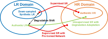
Figure 1: Domain interpretation of differences between supervised and unsupervised SR. A large degradation shift exists between the SR result and desired HR image, which is caused by applying a supervised network, which is pre-trained with synthetic LR images, to authentic LR images with degradation deviating.

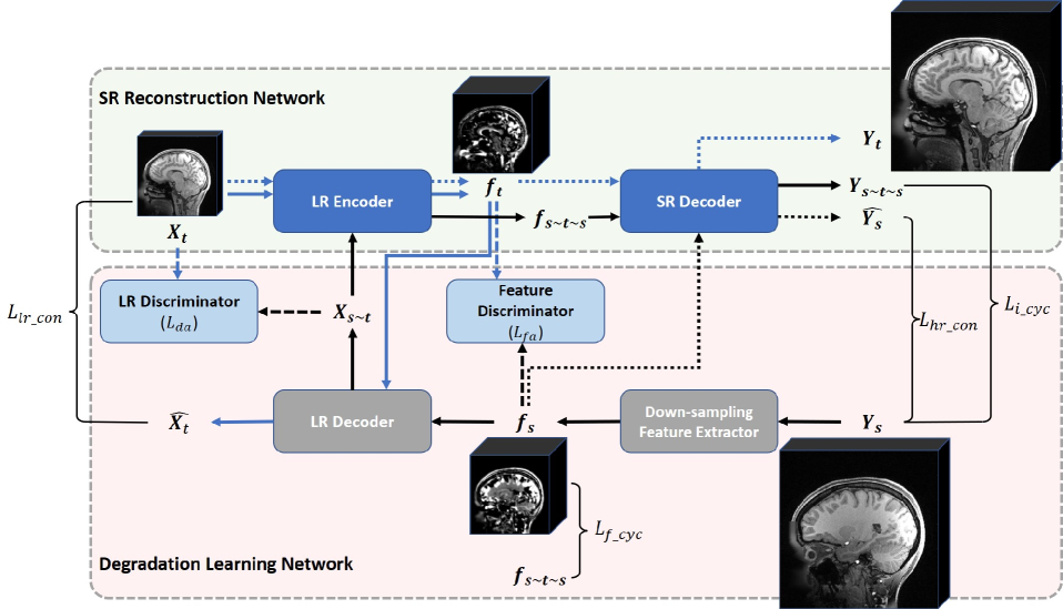
Figure 2: Pipeline of the UDEAN for 3D MRI super-resolution reconstruction. The network is fed with the unpaired or misaligned source group HR image patch $\textbf{Y}_{\textbf{s}}$ and the target group LR image patch $\textbf{X}_{\textbf{t}}$ in training. During the inference, only the target group LR image patch $\textbf{X}_{\textbf{t}}$ is fed in the network, and the SR image patch $\textbf{Y}_{\textbf{t}}$ is reconstructed.

2.1 Degradation Shift and SR Reconstruction with Unknown Degradation

Degradation shift, also known as domain gap in the real-world image SRR, was initially noticed in the blind SRR tasks, where the down-sampling parameters of the LR images were unknown [25]. In previous studies of real-world image SRR, the HR images were down-sampled with either a bicubic algorithm or specific Gaussian blurring kernels [25, 27, 28, 29, 31, 30, 26, 32, 33]. With these down-sampling algorithms, the parameters of the algorithms for the LR images in both training and inference datasets were known. They should be identical to guarantee the performance of the trained network [25]. However, the parameters of the down-sampling algorithms in the real world were normally unknown and very difficult to model [25]. Therefore, it’s impossible to guarantee the identical down-sampling for the LR images in both the training dataset and the inference dataset, and the difference between the degradation of the training and inference datasets resulted in a downgraded performance of the trained network in the inference[25], as shown in Fig. 1.

Similarly, in MRI SRR, $K$-space truncation is the most widely-used down-sampling algorithm to generate synthetic LR images [4, 5, 6, 7, 8, 9, 10]. With this algorithm, an HR image is transformed to its fake $K$-space using fast Fourier transformation (FFT), then the fake $K$-space is truncated based on the down-sampling factor. At last, the remained part of the fake $K$-space is transformed back to the synthetic LR image using inverse FFT (iFFT). However, the degradation shift between the synthetic and authentic LR images created in this process is still remained [17]. The method of $K$-space truncation is a highly simplified down-sampling model, which simulates the acquisition process of LR images based on the assumption that the $K$-spaces of both the HR and the LR images were fully sampled. However, to shorten the scan time in the clinical measurements, most of the protocols for both LR and HR images acquire $K$-spaces, which are under-sampled in several different manners, including partial Fourier in phase-encoding and/or slice-encoding direction, parallel imaging, elliptical $K$-space, etc. Most of these under-sampling processes are difficult to simulate accurately since many of the key parameters are unknown. Besides, some other factors also lead to unpredictable differences between the degradation representations of synthetic and authentic LR images, such as the varied signal-to-noise ratio caused by different signal intensity distribution of the $K$-spaces or different tuning of transmission/receiving chain.

Therefore, unsupervised SRR can be a promising solution when the degradation shift exists. Several methods have been proposed to tackle this problem. These methods can be categorized into three types: the generative network-based domain transfer methods [21, 22, 23], the blurring kernel-based methods [25, 27, 28, 29, 31, 30, 26], and contrastive learning [32, 33]. Since the LR images in MRI were not down-sampled with either bicubic or Gaussian blurring kernels, the blurring kernel-based methods are incompatible with the MRI SRR. Besides, contrastive learning requires positive and negative training samples, which are difficult to acquire, making this method not applicable in the MRI SRR. Therefore, a network with degradation adaptation based on the domain transfer method was built for SRR from LR images with unknown degradation.

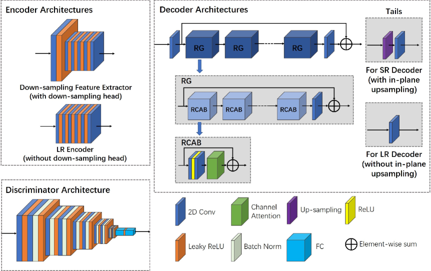
Figure 3: Detailed structures of network components. The encoders are constructed with 6 convolutional layers, each followed by a Leaky ReLU layer. The decoders adopt the TS-RCAN backbone. The VGG network is employed as the discriminator.

2.2 Network Architecture of the UDEAN

As to the unsupervised training, the image from the source and target groups are used in the training process. The images from the target group are the LR images that will be upsampled to reconstruct the SR images. The images from the source group provide the HR images with the style that the SR images expect. As shown in Fig. 2, the HR MRI image $\textbf{Y}_{\textbf{s}}$ from the source group and LR MRI image $\textbf{X}_{\textbf{t}}$ from the target group are either misaligned or unpaired, and there is not any ground truth HR image to calculate any pixel-wise or structural losses with the generated SR image. Noting that misaligned LR and HR images can be considered a special case of unpaired data, where the LR image contains similar structural information as the HR image but is not pixel-wise aligned. Therefore, the training is still not applicable in a supervised manner.

Therefore, we propose an unsupervised degradation adaptation network - UDEAN, whose architecture is shown in Fig. 2. The network contains two components: a degradation learning network and an SR Reconstruction network. There are two modules in the degradation learning network. The first module is a degradation mapping module, colored in gray as shown in Fig. 2. This module contains a down-sampling feature extractor and an LR decoder. The second module is an identification module consisting of an LR discriminator and a feature discriminator, as shown in Fig. 2 in light blue color. The SRR network includes an LR encoder and an SR decoder (colored in deep blue). It is expected to reconstruct SR images with comparable image quality with the HR images of the source group from the LR images of the target group.

As indicated along the black solid line, $\textbf{Y}_{\textbf{s}}$ is fed to a learnable down-sampling feature extractor to extract the down-sampled feature map $f_{s}$ of the source group. Such a feature map contains a generic degradation representation from HR to LR images. Then, the down-sampled LR image $X_{{s}\sim{t}}$, which contains a comparable degradation representation of the target group LR image $\textbf{X}_{\textbf{t}}$, is generated by the LR decoder. Then the feature map $f_{{s}\sim{t}\sim{s}}$ of $X_{{s}\sim{t}}$ is extracted using an LR encoder and generates the SR image $Y_{{s}\sim{t}\sim{s}}$ using an SR decoder. As the reconstructed SR image $Y_{{s}\sim{t}\sim{s}}$ and HR image in source group $\textbf{Y}_{\textbf{s}}$ are expected to be identical, and the feature map $f_{{s}\sim{t}\sim{s}}$ and $f_{s}$ should likewise contain comparable context, two cycle-losses (HR image and feature cycle-losses) are calculated for such purposes. Two consistency losses are also involved in making the training more stable. The LR encoder and LR decoder are trained by minimizing the target group error between $\textbf{X}_{\textbf{t}}$ and the LR image $\hat{X_{t}}$ decoded from $f_{t}$ along the blue solid line. Similarly, the down-sampling feature extractor and SR decoder are trained by minimizing the source group error between $\textbf{Y}_{\textbf{s}}$ and SR image $\hat{Y_{s}}$ reconstructed from $f_{s}$ along the black dotted line.

Since the network is expected to learn the specific degradation representation from the HR images in the source group to the LR images in the target group, an LR discriminator and a feature discriminator are employed. The former is trained to distinguish between the target group LR image $\textbf{X}_{\textbf{t}}$ and the LR image $X_{{s}\sim{t}}$ reconstructed from source group feature. The second discriminator is trained to distinguish between the feature $f_{t}$ retrieved from the target group LR and $f_{s}$. The discriminators have been trained alternately with the degradation mapping module and SRR network. The UDEAN can adapt from the source group to the specific degradation representation in the target group as long as the discriminators are deceived.

Only the trained LR encoder and SR decoder are required during the inference step, as shown along the blue dotted line in Fig. 2. The target group LR MRI image $\textbf{X}_{\textbf{t}}$ is encoded into the feature map, then the target group SR MRI image $\textbf{Y}_{\textbf{t}}$ is generated accordingly.

2.3 Loss Functions

In our experiments, we employed three types of loss functions, which are the L1 loss, the structural similarity (SSIM) loss [34][44] and the adversarial loss:

$$L_{1}(x,y)=\frac{1}{N}\sum_{i=1}^{N}\lvert x-y\rvert$$ (1)

$$L_{SSIM}(x,y)=\frac{1}{N}\sum_{i=1}^{N}\mid 1-SSIM(x,y)^{2}\mid$$ (2)

$$L_{adv}(x)=\frac{1}{N}\sum_{i=1}^{N}\sqrt{(D(x)-1)^{2}}$$ (3)

where the batch size is $N$, $x$ and $y$ represent the generated SR image and ground truth HR images, and $D(\cdot)$ represents the discriminator. To stabilize the training procedure, we use the least square loss [35] for the adversarial loss in our model instead of the negative log-likelihood [36].

As mentioned in the previous section, the two-cycle losses are used to guide the cross-domain restoration of the $Y_{{s}\sim{t}\sim{s}}$. The image cycle loss is calculated as a weighted sum of the L1 loss and SSIM loss between $Y_{{s}\sim{t}\sim{s}}$ and $\textbf{Y}_{\textbf{s}}$, and the adversarial loss of $Y_{{s}\sim{t}\sim{s}}$. The feature cycle loss is calculated as the L1 loss between $f_{{s}\sim{t}\sim{s}}$ and $f_{s}$:

$$L_{i\_cyc}=L_{1}(Y_{{s}\sim{t}\sim{s}},\textbf{Y}_{\textbf{s}})+\alpha*L_{SSIM}(Y_{{s}\sim{t}\sim{s}},\textbf{Y}_{\textbf{s}})$$ (4)

$$+\beta*L_{adv}(Y_{{s}\sim{t}\sim{s}})$$

$$L_{f\_cyc}=L_{1}(f_{{s}\sim{t}\sim{s}},f_{s})$$ (5)

Moreover, the consistency losses are used to restrain the restoration of $\hat{Y_{s}}$ and $\hat{X_{t}}$ within the source and target domain, respectively. They are calculated as a weighted sum of L1, SSIM, and adversarial loss:

$$L_{hr\_con}=L_{1}(\hat{Y_{s}},\textbf{Y}_{\textbf{s}})+\alpha*L_{SSIM}(\hat{Y_{s}},\textbf{Y}_{\textbf{s}})$$ (6)

$$+\beta*L_{adv}(\hat{Y_{s}})$$

$$L_{lr\_con}=L_{1}(\hat{X_{t}},\textbf{X}_{\textbf{t}})+\alpha*L_{SSIM}(\hat{X_{t}},\textbf{X}_{\textbf{t}})$$ (7)

$$+\beta*L_{adv}(\hat{X_{t}})$$

where $\alpha$ and $\beta$ are the weights of the SSIM and adversarial loss, respectively. We set $\alpha=0.5$ and $\beta=0.01$ in our experiments.

Furthermore, the DA losses in image space ($L_{da}$) and in latent feature space ($L_{fa}$), which stemmed from the LR discriminator and the feature discriminator, are used to guide the network approaching the distributions of the LR images and the features extracted from different domains:

$$L_{da}(X_{{s}\sim{t}},\textbf{X}_{\textbf{t}})=\frac{1}{N}\sum_{i=1}^{N}\lvert D_{da}(X_{{s}\sim{t}})-0.5\rvert$$ (8)

$$+\frac{1}{N}\sum_{i=1}^{N}\lvert D_{da}(\textbf{X}_{\textbf{t}})-0.5\rvert$$

$$L_{fa}(f_{t},f_{s})=\frac{1}{N}\sum_{i=1}^{N}\lvert D_{fa}(f_{t})-0.5\rvert$$ (9)

$$+\frac{1}{N}\sum_{i=1}^{N}\lvert D_{fa}(f_{s})-0.5\rvert$$

As a result, the end-to-end training loss for the generators in our network is defined as

$$Loss_{G}=\lambda_{1}*L_{i\_cyc}+\lambda_{2}*L_{f\_cyc}+\lambda_{3}*L_{hr\_con}$$ (10)

$$+\lambda_{4}*L_{lr\_con}+\lambda_{5}*L_{da}+\lambda_{6}*L_{fa}$$

where $\lambda_{1}$ to $\lambda_{6}$ are the weights of the loss components. We set $\lambda_{1,3,4}=1$ and $\lambda_{2,5,6}=0.1$ in our experiments for the best performance.

2.4 Dataset and Data Pre-processing

In this study, we used two public datasets:

2.4.1 Human Connectome Project (HCP) dataset

The T1w images from the HCP dataset, which consists of images from 1113 healthy participants [37]. The T1w images were acquired in the sagittal plane with 3D MPRAGE, $TR=2400ms,TE=2.14ms,TI=1000ms,FA=8,FOV=224mm,rBW=210Hz/Px$, the matrix size was $320\times 320\times 256$ with isotropic of resolution $0.7mm$, and $\times 2$ GRAPPA in phase encoding direction was activated. To shorten the training time, we randomly selected 300 participants for our study.

2.4.2 Brain Tumor Segmentation Challenge 2020 (BraTS) dataset

The contrast-enhanced T1w (T1CE) images from the BraTS dataset, which consists of images from 369 participants with brain tumors[38, 39, 40]. The T1CE images were acquired in the axial plane, the matrix size was $240\times 240\times 155$ with isotropic resolution $1.0mm$. To shorten the training time, we randomly selected 300 participants for our study.

Our experiments involved four data groups: the source, target, validation, and test group. The source and target groups were used to train the neural networks, the validation group was used to monitor the networks’ performance during training, and the test group was used to evaluate the networks after training. We randomly selected 120/120/30/30 participants from the HCP dataset for the source, target, validation, and test group. The target group contains only LR images, which were down-sampled from the HR images by 3D $K$-space truncation with scale factors of $2\times 2\times 1$ and $2\times 2\times 2$ [4, 5, 6, 7, 2, 8, 3, 9, 10]. The source group contained only HR images from 120 participants and differed between the experiments with misaligned/unpaired HR and LR images. For the unpaired SRR, the participants of the source group were isolated from the other three groups; For the misaligned SRR, the source group shared the same participants with the target group, and the HR images were distorted with certain deformation patterns.

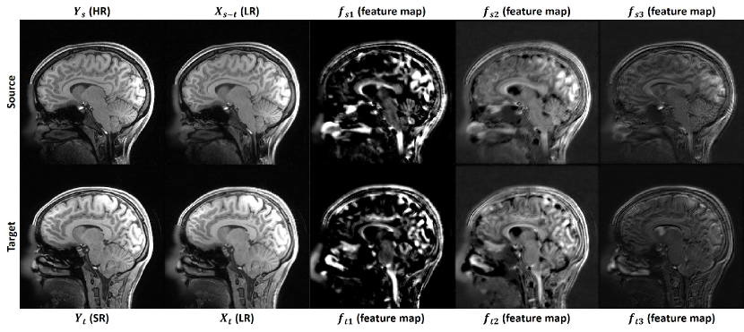
Figure 4: Illustration of the degradation adaptation and feature extraction. Images with similar anatomical structures were selected from different participants in the source group (in the top row) and the target group (in the bottom row). $\textbf{Y}_{\textbf{s}}$ was the HR image from the source group, and $\textbf{Y}_{\textbf{t}}$ was the SR image reconstructed using the LR image ($X_{t}$) from the target group. $X_{{s}\sim{t}}$ was the LR image degraded from $\textbf{Y}_{\textbf{s}}$ by the degradation learning network, and its image quality was comparable to $X_{t}$. $f_{s1}$ to $f_{s3}$ and $f_{t1}$ to $f_{t3}$ were the examples of the feature maps extracted from $\textbf{Y}_{\textbf{s}}$ and $X_{t}$, respectively. Highly consistent patterns could be found between the feature maps of the source group and the target group, revealing the effectiveness of the degradation adaptation in the latent feature space.

Specifically, for the SRR from misaligned LR and HR image pairs, the participant movement between the acquisition of HR and LR images was simulated by adopting mild rigid movement and non-rigid geometric deformation to the HR images. The rigid movement was performed by random rotation of the image volumes by 0 to 2 degrees around the head-feet (H-F) axis and the left-right (L-R) axis and random translation by 0 to 2 voxels in H-F and head-feet L-R directions. The geometric deformation was achieved by randomly shrinking the whole image volumes by 0 to 2 voxels in anterior-posterior (A-P) and L-R directions, resulting in a 0.7 to 0.9% change in the objects’ sizes. Each dataset was scaled to the range of 0 to 1, and to save computation resources, the LR and HR images were cropped into 3D patches of sizes $64\times 64\times 3$ and $128\times 128\times 3$ for the scale factor of $2\times 2\times 1$, and $64\times 64\times 3$ and $128\times 128\times 6$ for the scale factor of $2\times 2\times 2$, respectively.

Table 1: Quantitative results of ablation study for MRI SRR with misaligned LR and HR images of the HCP dataset and scale factor of $2\times 2\times 2$.

	Supervised without	Supervised with	Unsupervised with	Unsupervised with	Unsupervised with
	Rigid-Registration	Rigid-Registration	DA in Feature Space	DA in Image Space	DA in Both Spaces
SSIM	$0.8939\pm 0.0140$	$0.9025\pm 0.0116$	$0.9162\pm 0.0104$	$0.9229\pm 0.0093$	$\mathbf{0.9247\pm 0.0097}$
PSNR	$32.7886\pm 1.5546$	$32.7823\pm 1.5013$	$33.5224\pm 1.6849$	$33.5642\pm 1.7719$	$\mathbf{34.2729\pm 1.8080}$

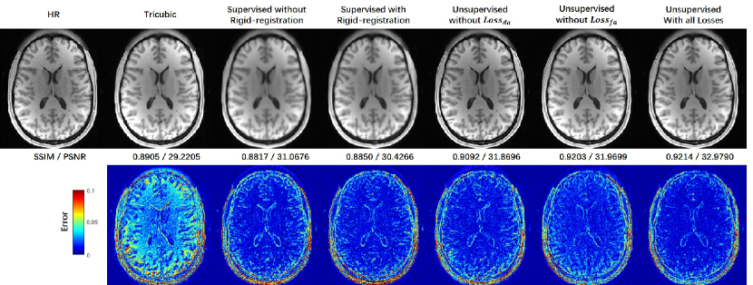
Figure 5: Comparison of reconstructed SR images and error maps of supervised learning and different configurations of the UDEAN with misaligned LR and HR image pairs of the HCP dataset and the scale factor of $2\times 2\times 2$ in the axial plane. The SR images reconstructed using supervised learning are highly blurry. The

2.5 Implementation Details

The detailed structures of our model components are shown in Fig. 3. For the encoders, we used 6 convolution layers with Leaky ReLU between every two layers, and the down-sampling feature extractor down-samples the input HR image to the same size as the LR image. We used the TS-RCAN [16] with 5 residual groups (RG) and 5 residual blocks (RCAB) in each RG as the backbone of the decoders, and VGG [43] as the discriminator for the UDEAN. TS-RCAN is modified from RCAN [41, 42] to conduct 3D MRI SR tasks with low consumption of computation resources and short inference time.

The networks were trained on a workstation equipped with an Nvidia Quadro A6000. For all deep learning experiments, we used Pytorch 1.9 as the back end. In each training batch, eight LR patches were randomly extracted as inputs. We trained our model for 30 epochs using the ADAM optimizer with $\beta_{1}=0.9$, $\beta_{2}=0.99$, and $\epsilon=10^{-8}$, and a Cosine-decay learning rate was applied from $10^{-4}$ to $10^{-8}$. The image pre-processing of down-sampling, deformation, and cropping and the post-processing and metrics calculation were performed with Matlab 2020a. The rigid image registration was performed on Amira 3D with metrics of extended mutual information.

The image quality was evaluated by the most widely-used metrics, signal-to-noise ratio (PSNR) and structure similarity index (SSIM) [4, 6, 7, 2, 8, 3, 10]. The higher values of PSNR and SSIM represent better performance. Unlike regular image SRR studied in computer vision research, we didn’t adopt any perceptual metrics since structural accuracy is more important than the pure perceptual effect in clinical diagnosis and image-guided treatments.

3 Experiments and Results

3.1 Illustration of Degradation Adaptation

As shown in Fig. 4, images with similar anatomical structures were selected from different participants in the source group (in the top row) and the target group (in the bottom row). $\textbf{Y}_{\textbf{s}}$ was the HR image from the source group and $\textbf{Y}_{\textbf{t}}$ was the SR image reconstructed using the LR image ($X_{t}$) from the target group. $X_{{s}\sim{t}}$ was the LR image down-sampled from $\textbf{Y}_{\textbf{s}}$ by the degradation learning network of UDEAN. $X_{t}$ and $X_{{s}\sim{t}}$ had highly comparable image quality, this was achieved by the degradation adaptation mechanism of the network. $f_{s1}$ to $f_{s3}$ and $f_{t1}$ to $f_{t3}$ were the feature maps extracted from $\textbf{Y}_{\textbf{s}}$ and $X_{t}$, respectively. The patterns in the feature maps of the source group and the target group were highly consistent, revealing the effectiveness of the degradation adaptation in the latent feature space. With certain consistency between the source group and the target group in both the image space and the latent feature space, UDEAN was able to reconstruct SR images from LR images from the target group with comparable quality to the HR images from the source domain.

3.2 Ablation Study of the UDEAN

We evaluated our network in various configurations on the same task of SRR for misaligned LR and HR datasets to find the best performance. The effect of DA in the image space and latent feature space was evaluated. Besides, we compared our network to the same backbone network trained in the supervised strategy with the misaligned training data to reveal the effect of the degradation-learning modules. As shown in Table 1, all the configurations of the UDEAN outperformed the supervised learning using the same generator by over 0.014/0.74 dB in SSIM/PSNR using misaligned LR and HR image from the HCP dataset with the scale factor of $2\times 2\times 2$. Among the configurations of the UDEAN, the performance was downgraded by 0.009/0.75 dB or 0.002/0.71 dB in SSIM/PSNR when DA in only latent feature space or image space was applied, respectively.

Furthermore, Fig. 5 shows the visual effect of the reconstructed SR images and the error maps to the HR images. The SR image reconstructed by the supervised methods were highly blurry either with or without rigid image registration. On the contrary, the quality of SR images reconstructed by the UDEAN was significantly improved even with DA only in latent feature space or image space. The errors of the reconstructed anatomical structures were further reduced when DA in both domains was applied in the training process.

Table 2: Quantitative comparison with the state-of-the-art unsupervised networks for MRI SRR with misaligned and unpaired LR and HR images

Dataset	Scale Factor	Method	Misaligned or Unpaired	SSIM	PSNR
HCP	$2\times 2\times 2$	Tricubic	N/A	$0.8981\pm 0.0106$	$31.5862\pm 1.8520$
		ZSSR [18]		$0.8994\pm 0.0163$	$33.0213\pm 2.2054$
		DASR [23]	Unpaired	$0.8931\pm 0.0094$	$32.3309\pm 1.4671$
		Pseudo SR [22]		$0.8931\pm 0.0116$	$31.0407\pm 1.8816$
		Blind-SR [24]		$0.9132\pm 0.0100$	$33.0695\pm 1.4656$
		$\mathbf{UDEAN(ours)}$		$\mathbf{0.9242\pm 0.0083}$	$\mathbf{33.5159\pm 1.7234}$
		DASR [23]	Misaligned	$0.8946\pm 0.0091$	$32.2544\pm 1.4658$
		Pseudo SR [22]		$0.8962\pm 0.0086$	$32.0267\pm 1.5950$
		Blind-SR [24]		$0.9149\pm 0.0091$	$33.1597\pm 1.5693$
		$\mathbf{UDEAN(ours)}$		$\mathbf{0.9247\pm 0.0097}$	$\mathbf{34.2729\pm 1.8080}$
	$2\times 2\times 1$	Tricubic	N/A	$0.9227\pm 0.0088$	$33.6545\pm 1.8492$
		ZSSR [18]		$0.9412\pm 0.0106$	$\mathbf{36.0848\pm 2.4098}$
		DASR [23]	Unpaired	$0.9137\pm 0.0084$	$33.6732\pm 1.4502$
		Pseudo SR [22]		$0.9244\pm 0.0076$	$33.8122\pm 1.6044$
		Blind-SR [24]		$0.9325\pm 0.0081$	$34.9527\pm 1.7325$
		$\mathbf{UDEAN(ours)}$		$\mathbf{0.9371\pm 0.0078}$	$\mathbf{35.1688\pm 1.8195}$
		DASR [23]	Misaligned	$0.9192\pm 0.0082$	$33.9043\pm 1.6386$
		Pseudo SR [22]		$0.9228\pm 0.0080$	$34.0500\pm 1.6694$
		Blind-SR [24]		$0.9395\pm 0.0071$	$35.0236\pm 1.8130$
		$\mathbf{UDEAN(ours)}$		$\mathbf{0.9455\pm 0.0072}$	$\mathbf{35.5182\pm 2.2839}$
BraTS	$2\times 2\times 2$	Tricubic	N/A	$0.9073\pm 0.0196$	$31.2470\pm 1.9187$
		ZSSR [18]		$0.9001\pm 0.0464$	$29.6156\pm 3.1528$
		DASR [23]	Unpaired	$0.9334\pm 0.0141$	$30.5198\pm 2.0642$
		Pseudo SR [22]		$0.8978\pm 0.0129$	$26.4210\pm 0.8741$
		Blind-SR [24]		$0.9434\pm 0.0121$	$31.2900\pm 2.2618$
		$\mathbf{UDEAN(ours)}$		$\mathbf{0.9471\pm 0.0096}$	$\mathbf{31.4467\pm 2.3570}$
		DASR [23]	Misaligned	$0.9377\pm 0.0151$	$31.1546\pm 2.0495$
		Pseudo SR [22]		$0.9378\pm 0.0150$	$31.0804\pm 1.9391$
		Blind-SR [24]		$0.9360\pm 0.0120$	$31.2894\pm 1.9017$
		$\mathbf{UDEAN(ours)}$		$\mathbf{0.9513\pm 0.0133}$	$\mathbf{32.0435\pm 2.2796}$
	$2\times 2\times 1$	Tricubic	N/A	$0.9299\pm 0.0151$	$34.8846\pm 2.2722$
		ZSSR [18]		$0.9514\pm 0.0156$	$33.2469\pm 3.6422$
		DASR [23]	Unpaired	$0.9462\pm 0.0149$	$34.4395\pm 1.8905$
		Pseudo SR [22]		$0.9397\pm 0.0150$	$34.0382\pm 1.9015$
		Blind-SR [24]		$0.9510\pm 0.0156$	$35.3235\pm 2.0213$
		$\mathbf{UDEAN(ours)}$		$\mathbf{0.9551\pm 0.0166}$	$\mathbf{35.4973\pm 2.2433}$
		DASR [23]	Misaligned	$0.9461\pm 0.0167$	$34.5953\pm 2.0557$
		Pseudo SR [22]		$0.9463\pm 0.0162$	$34.5560\pm 1.9037$
		Blind-SR [24]		$0.9558\pm 0.0158$	$36.1029\pm 2.2270$
		$\mathbf{UDEAN(ours)}$		$\mathbf{0.9629\pm 0.0163}$	$\mathbf{36.7631\pm 2.3787}$

3.3 Comparison with the State-of-the-Art Unsupervised Methods

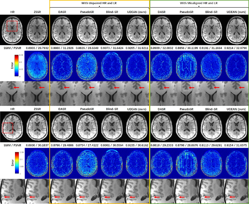
Figure 6: Qualitative comparison of the UDEAN with the state-of-the-art unsupervised networks in visual effect and error maps in the axial plane with the HCP dataset and the scale factor of $2\times 2\times 2$. The arrows point out the small structures that UDEAN reconstructed with higher accuracy than the other networks.

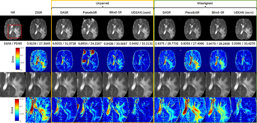
Figure 7: Qualitative comparison of the UDEAN with the state-of-the-art unsupervised networks in visual effect and error maps in the axial plane with the BraTS dataset and the scale factor of $2\times 2\times 2$. UDEAN achieved the lowest error in the region of the lesion.

We implemented other state-of-the-art unsupervised networks, including ZSSR [18], DASR [23], PseudoSR[22], and Blind-SR[24], as the baseline. All these networks used the same backbone as the UDEAN for both generators and discriminators and trained with identical training setups, including training datasets and hyperparameters, for fair comparisons. For inference, UDEAN and DASR used a single upsampling network with the same structure. As a result, the inference process for UDEAN and DASR consumed identical computation resources, including the same number of network parameters, number of operations, GPU consumption, and inference time. Blind-SR and PseudoSR used another network for style transfer in addition to the upsampling network, thus consuming approximately twice as many computation resources as the other two. The numerical results in Table 2 reveal that the UDEAN outperformed all the above-mentioned networks for MRI SRR from both misaligned and unpaired training data, which are from two public datasets with different contrasts and two scale factors. Specifically, for the HCP dataset and both scale factors, UDEAN outperformed the other networks in the SSIM and PSNR values for both misaligned and unpaired training data, only except the PSNR value of ZSSR with the scale factor of $2\times 2\times 1$. For the BraTS dataset, the UDEAN also outperformed all the other networks with the highest SSIM and PSNR values in most of the experiments.

As to the qualitative comparison shown in Fig. 6 for the SRR of the HCP dataset with a scale factor of $2\times 2\times 2$, ZSSR generated highly blurry images, although its metrics values are higher than DASR and PseudoSR in some cases. Among all the images, the ones reconstructed by UDEAN achieved the lowest errors as shown in the error maps, and the best accuracy in small anatomical structures pointed out by the red arrows. Also shown in Fig. 7 for the SRR with the BraTS dataset and the scale factor of $2\times 2\times 2$, UDEAN achieved better accuracy than the other networks in the structures of lesions, which may improve the accuracy of the assessment of the lesions and the therapy based on the reconstructed SR images.

4 Discussion

4.1 Practicality in Clinical Settings

In real clinical settings, perfectly paired and aligned authentic LR and HR images are difficult to acquire due to patient movements. Besides, in-vivo images are mostly acquired with either LR or HR images in clinical settings because of high time consumption and cost. Lacking paired and aligned LR and HR images raises challenges in implementing supervised SRR methods. Our experimental results revealed that supervised methods could not provide acceptable image quality if the LR and HR images in the training datasets were not perfectly aligned. Even with rigid image registration, the inference results were still unsatisfactory if there was a tiny geometric deformation between the LR and HR images. Besides, considering the change of the object size in our experiments was between 0.7% and 0.9%, which was far beyond the accuracy of 90% DSC achieved by the latest deep learning-based deformable image registration [15], the deformable image registration algorithms are not helpful in solving such tiny misalignment of soft tissues. Therefore, previous studies adopted synthetic LR images generated from HR images with certain down-sampling algorithms as the input of the network [4, 6, 7, 2, 8, 3, 10]. However, the degradation shift between the artificial down-sampling and the real degradation from authentic HR to LR images downgrades the performance of the trained networks when they are used for SRR from authentic LR images [17]. Therefore, unsupervised networks can be the possible solution to these problems.

Previously proposed unsupervised networks were designed for 2D real-world images [18, 21, 23, 22]. However, medical images are mostly in 3D form, containing through-slice information. Therefore, we adopted the TS-RCAN [16], which is a low-cost network for 3D SRR with enhanced performance, as the backbone of the UDEAN to process 3D medical images. And comparing to the other unsupervised method, the UDEAN learned the degradation representation in both image space and the latent feature space, thus achieving better performance.

4.2 Effect of Degradation Representation Learning

The degradation representation learning of the UDEAN was a specific type of domain adaptation, which transferred HR images of the source domain to the LR images of the target domain. As illustrated in the result section, UDEAN was able to down-sample the HR image from the source group to the LR image, which had a comparable quality to the target group. The consistency in the latent feature spacce between the source group and the target group further helped the network with improved accuracy. The ablation study also revealed the effects of domain adaptations, which guided the network to learn the degradation representation in both image and latent feature space. The experimental results showed the advantage of UDEAN to the supervised learning approach on misaligned LR and HR images. When the LR and HR images of the training datasets were not perfectly aligned, the supervised methods failed to provide acceptable image quality. Besides, the ablation study also revealed the effect of degradation representation learning in both image and latent feature space. The network could reconstruct the SR images without either $Loss_{da}$ or $Loss_{fa}$. However, the absence of $Loss_{da}$ or $Loss_{fa}$ downgraded the network’s performance, showing the benefit of degradation representation learning in both the image space and the latent feature space.

4.3 Comparison of Different Domain Transfer Strategies

Regarding the other state-of-the-art unsupervised networks, the ZSSR, as a network without domain transfer, learned the degradation representation between LR images and the lower resolution images, which were down-sampled from LR images, and used the learned degradation representation to reconstruct the SR images from the LR images [18]. However, there was a large gap between the learned degradation and the degradation from HR images to the LR images, thus leading to downgraded performance, particularly with large-scale factors. Although it achieved high metrics values in a few cases, the reconstructed SR images were highly blurry as shown in our results, and cannot meet the quality required in clinics.

Most of the unsupervised networks with domain transfer are derived from the CycleGAN. As one of the latest unsupervised SR approaches, the DASR learns the degradation representation by down-sample the HR images of the source domain to the LR images in the target domain, and domain distance maps in the image space are generated simultaneously, which are subsequently used to reconstruct SR images [23]. However, this learning strategy was not in an end-to-end fashion, so the early stop when the down-sampling network (DSN) reached the best performance on the validation dataset was not applicable. The DSN could be overfitted to the training dataset, making the whole network difficult to be trained and optimized, and the learned degradation representation fits the reconstruction procedure hardly. As a result, the inaccuracies in the DASR’s reconstructed SR MRI images are still massively visible.

The PseudoSR is another most recent approach to an unsupervised SRR network. It transfers the LR image of the target domain to the source domain, where the LR images are downgraded from HR images with a predefined algorithm (normally bicubic or Gaussian blurring). Then the SR images are reconstructed from down-sampled LR images [22]. The experimental results showed that the PseudoSR could achieve neither high metrics values nor satisfactory qualitative image quality. Despite the adaptation of latent feature space, another main difference between the UDEAN and the PseudoSR was that the UDEAN transfers the source domain HR images to the target domain and learns the mapping of the LR images from the target domain to the HR images in the source domain. On the contrary, the PseudoSR transfers the target domain LR images to the source domain and learns the mapping of the LR images from the source domain to the HR images in the source domain. The ablation study results showed the advantage of the former scheme even with the absence of feature space adaptation. And with the latter approach, more detailed structures were missing in the reconstructed SR images.

Blind-SR is another variation of CycleGAN, which has been applied to MRI SRR. It shares a similar scheme with the PseudoSR, which transfers the LR image of the target domain to the source domain, whose images are downsampled with bicubic or nearest algorithms. Therefore, it confronted a similar problem with PseudoSR, with whom lots of detailed structure information were lost. Besides, the Blind-SR was not trained in an end-to-end fashion either. Its two components were trained separately, making it face similar difficulties in optimizing the network like DASR.

Besides the differences in the domain transfer strategies, UDEAN and DASR utilized a single upsampling network for the inference, whereas PseudoSR and Blind-SR used another style transfer network in addition to the upsampling network. As a result, the computation resources consumed by UDEAN were identical to DASR and approximately 50% less than PseudoSR and Blind-SR.

4.4 Limitations and Future Works

Despite the promising results of the UDEAN, we acknowledge certain limitations to this study. We only tested the UDEAN on MRI images of brains, where the geometric deformation is normally mild in real clinics, and the LR images were synthetically generated from HR images. Abdominal and musculoskeletal imaging normally suffer from more severe geometric deformation of soft tissues due to irresistible patient movements. Thus, the UDEAN can be the best solution in these scenarios and will be investigated in our future study. Besides, public datasets containing authentic LR and HR images of abdominal and musculoskeletal imaging are unavailable. Therefore the misaligned or unpaired LR and HR images still need to be artificially generated. This study focused on investigating the potential of SRR using networks trained by misaligned or unpaired LR and HR images, the datasets we used in our experiments were still applicable to our experiments. In our future study, the performance of the UDEAN trained with authentic LR and HR images will be investigated.

5 Conclusion

In this manuscript, we propose the UDEAN as an unsupervised degradation adaption network that adaptively learns the degradation representation between misaligned or unpaired LR and HR MRI data in both image and latent feature spaces. The UDEAN applies SRR in an end-to-end fashion, making the network easy to train and optimize. The DA mechanism adopted by the UDEAN also shows advantages over the previously used domain transfer methods, thus minimizing errors in the reconstructed SR images. Our experimental results showed that the UDEAN alleviated the problem of lacking paired authentic LR and HR images, achieved enhanced image quality for SRR, and outperformed the other state-of-the-art networks. Therefore, the UDEAN is a promising solution for SRR in clinical settings when perfectly aligned LR and HR image pairs are unavailable.

References

- [1] S. Wang et al., “Accelerating magnetic resonance imaging via deep learning.” Proc. IEEE Int. Symp. Biomed. Imag., Apr. 2016, pp. 514–517.
- [2] X. Zhao, Y. Zhang, T. Zhang, and X. Zou, “Channel splitting network for single MR image super-resolution,” IEEE Trans. Image Process., vol. 28, no. 11, pp. 5649–5662, 2019.
- [3] Y. Zhang, K. Li, K. Li, and Y. Fu, “MR image super-resolution with squeeze and excitation reasoning attention network,” Proc. IEEE/CVF Conf. Comput. Vis. Pattern Recognit. (CVPR), Jun. 2021, pp. 13425–13434.
- [4] C. H. Pham, A. Ducournau, R. Fablet, and F. Rousseau, “Brain MRI super-resolution using deep 3D convolutional networks,” Proc. IEEE Int. Symp. Biomed. Imag., Apr. 2017, pp. 197–200.
- [5] C. H. Pham et al., “Multiscale brain MRI super-resolution using deep 3D convolutional networks, ” Comput. Med. Imaging. Graph., vol. 77, 101647, 2019.
- [6] Y. Chen, Y. Xie, Z. Zhou, F. Shi, A. G. Christodoulou, and D. Li, “Brain MRI super resolution using 3D deep densely connected neural networks,” Proc. IEEE Int. Symp. Biomed. Imag., Apr. 2018, pp. 739–742.
- [7] Y. Chen, F. Shi, A. G. Christodoulou, Y. Xie, Z. Zhou, and D. Li, “Efficient and accurate MRI super-resolution using a generative adversarial network and 3D multi-level densely connected network,” Proc. Int. Conf. Med. Image Comput. Comput.-Assist. Intervent., Sep. 2018, pp. 91–99.
- [8] Y. Sui, O. Afacan, A. Gholipour, and S. K. Warfield, “Learning a gradient guidance for spatially isotropic MRI super-resolution reconstruction,” Proc. Int. Conf. Med. Image Comput. Comput.-Assist. Intervent., Oct. 2020, pp. 136–146.
- [9] Q. Lyn et al., “Multi-Contrast Super-Resolution MRI Through a Progressive Network,” IEEE Trans. Med. Imag, vol. 39, no. 9, pp. 2738-2749, 2020.
- [10] C. Feng, H. Fu, S. Yuan, and Y. Xu, “Multi-contrast mri super-resolution via a multi-stage integration network,” Proc. Int. Conf. Med. Image Comput. Comput.-Assist. Intervent., Sep. 2021, pp. 140–149.
- [11] Z. Sui, O. Afacan, C. Jaimes, A. Gholipour, and S. K. Warfield, “Scan-Specific Generative Neural Network for MRI Super-Resolution Reconstruction,” IEEE Trans. Med. Imag, vol. 41, no. 6, pp. 2738-2749, 2022.
- [12] C. Zhao, B. E. Dewey, D. L. Pham, P. A. Calabbresi, D. S. Reich, and J. L. Prince, “SMORE: A Self-Supervised Anti-Aliasing and Super-Resolution Algorithm for MRI Using Deep Learning,” IEEE Trans. Med. Imag, vol. 40, no. 3, pp. 805-817, 2021.
- [13] Y. Sui, O. Afacan, A. Gholipour, and S. K. Warfield, “MRI super-resolution through generative degradation learning,” Proc. Int. Conf. Med. Image Comput. Comput.-Assist. Intervent., Sep. 2021, pp. 430–440.
- [14] C. Komninos et al., “Intra-operative oct (ioct) image quality enhancement: a super-resolution approach using high quality ioct 3d scans,” Ophthalmic Medical Image Analysis (OMIA), in Conjunction with MICCAI, vol. 12970, 2021, pp. 21–31.
- [15] A. Zakeri et al., “DragNet: Learning-based deformable registration for realistic cardiac MR sequence generation from a single frame,” Medical Image Analysis, vol. 83, 2023, doi: https://doi.org/10.1016/j.media.2022.102678.
- [16] H. Li and J. Liu, “3D High-Quality Magnetic Resonance Image Restoration in Clinics Using Deep Learning,” 2021, arXiv:2111.14259.
- [17] S. Laguna et al., “Super-resolution of portable low-field MRI in real scenarios: integration with denoising and domain adaptation,” Proc. Medical Imaging with Deep Learning, Apr. 2022.
- [18] A. Shocher, C. Nadav Cohen, and I. Michal, ““zero-shot” super-resolution using deep internal learning,” Proc. IEEE/CVF Conf. Comput. Vis. Pattern Recognit. (CVPR), Jun. 2018, pp. 3118–3126.
- [19] Y. Iwamoto, K. Takeda, Y. Li, A. Shiino, and Y. Chen, “Unsupervised MRI Super-Resolution Using Deep External Learning and Guided Residual Dense Network with Multimodal Image Priors,” 2020, arXiv:2008.11921.
- [20] J. Cui, K. Gong, P. Han, H. Liu, and Q. Li, “Unsupervised arterial spin labeling image superresolution via multiscale generative adversarial network,” Med. Phys., vol. 49, no. 4, pp. 2373-2385, 2022.
- [21] J. Zhu, T. Park, P. Isola, and A. A. Efros, “Unpaired image-to-image translation using cycle-consistent adversarial networks,” Proc. IEEE/CVF Conf. Comput. Vis. Pattern Recognit. (CVPR), Jul. 2017, pp. 2223–2232.
- [22] S. Maeda, “Unpaired image super-resolution using pseudo-supervision,” Proc. IEEE/CVF Conf. Comput. Vis. Pattern Recognit. (CVPR), Jun. 2020, pp. 291–300.
- [23] Y. Wei, S. Gu, Y. Li, R. Timofte, L. jin, and H. Song, “Unsupervised real-world image super resolution via domain-distance aware training,” Proc. IEEE/CVF Conf. Comput. Vis. Pattern Recognit. (CVPR), Jun. 2021, pp. 13385–13394.
- [24] H. Zhou, Y. Huang, Y. Li, Y. Zhou, and Y. Zheng, “Blind Super-Resolution of 3D MRI via Unsupervised Domain Transformation,” IEEE Journal of Biomedical and Health Informatics, vol. 27, no. 3, pp. 1409–1418, 2023.
- [25] A. Liu, Y. Liu, J. Gu, Y. Qiao, and C. Dong, “Blind image super-resolution: A survey and beyond,” IEEE Trans. Pattern Anal. Mach. Intell., 2022, doi: 10.1109/TPAMI.2022.3203009.
- [26] J. Gu, H. Lu, W. Zuo, and C. Dong, “Blind super-resolution with iterative kernel correction,” Proc. IEEE/CVF Conf. Comput. Vis. Pattern Recognit. (CVPR), Jun. 2019, pp. 1604–1613.
- [27] L. Xie, X. Wang, C. Dong, Z. Qi, and Y. Shan, “Finding discriminative filters for specific degradations in blind super-resolution,” Proc. Adv. Neural Inf. Process. Syst., vol. 34, 2021, pp. 51–61.
- [28] Z. Hui, J. Li, X. Wang, and X. Gao, “Learning the non-differentiable optimization for blind super-resolution,” Proc. IEEE/CVF Conf. Comput. Vis. Pattern Recognit. (CVPR), Jun. 2021, pp. 2093–2102.
- [29] M. Yamac, A. Baran, and N. Aakif, “Kernelnet: A blind super-resolution kernel estimation network,” Proc. IEEE/CVF Conf. Comput. Vis. Pattern Recognit. (CVPR), Jun. 2021, pp. 453–462.
- [30] K. Zhang, J. Liang, L. Van Gool, and R. Timofte, “Designing a practical degradation model for deep blind image super-resolution,” Proc. IEEE Int. Conf. Comput. Vis. (ICCV), Oct. 2021, pp. 4791–4800.
- [31] W. Zhang, G. Shi, Y. Liu, C. Dong, and X. Wu, “A Closer Look at Blind Super-Resolution: Degradation Models, Baselines, and Performance Upper Bounds,” Proc. IEEE/CVF Conf. Comput. Vis. Pattern Recognit. (CVPR), Jun. 2022, pp. 527–536.
- [32] L. Wang et al., “Unsupervised degradation representation learning for blind super-resolution,” Proc. IEEE Int. Conf. Comput. Vis. (ICCV), Oct. 2021, pp. 10581–10590.
- [33] J. Zhang, S. Lu, F. Zhan, and Y. Yu, “Blind image super-resolution via contrastive representation learning,” 2021, arXiv:2107.00708.
- [34] E. M. Masutani, B. Naeim, and H. Albert, “Deep learning single-frame and multiframe super-resolution for cardiac MRI,” Radiology, vol. 295, no.3, pp. 552–561, 2020.
- [35] X. Mao, Q. Li, H. Xie, R. Y. K. Raymond, and Z. Wang, “Multi-class generative adversarial networks with the L2 loss function,” 2016, arXiv:1611.04076.
- [36] I. Goodfellow et al., “Generative adversarial networks,” Commun. ACM, vol. 63, no. 11, pp. 139-144, 2020.
- [37] D. C. Van Essen et al., “The WU-Minn human connectome project: an overview,” Neuroimage, vol. 80 pp. 62-79, 2013.
- [38] B. Menze et al., “The multimodal brain tumor image segmentation benchmark (BRATS),” IEEE Trans. Med. Imag, vol. 34, no. 10, pp. 1993-2024, 2014.
- [39] C. T. Lloyd, S. Alessandro, and A. J. Tatem, “High resolution global gridded data for use in population studies,” Sci. Data, vol. 4, no. 1, pp. 1-17, 2017.
- [40] S. Bakas et al., “Identifying the best machine learning algorithms for brain tumor segmentation, progression assessment, and overall survival prediction in the BRATS challenge,” 2018, arXiv:1811.02629.
- [41] Y. Zhang, K. Li, K. Li, L. Wang, B. Zhong, and Y. Fu, “Image super-resolution using very deep residual channel attention networks,” Proc. Eur. Conf. Comput. Vis., Sep. 2018, pp. 286–301.
- [42] Z. Lin et al., “Revisiting rcan: Improved training for image super-resolution,” 2022, arXiv:2201.11279.
- [43] K. Simonyan, and Z. Andrew, “Very deep convolutional networks for large-scale image recognition,” 2014, arXiv:1409.1556.
- [44] Z. Wang, A. C. Bovik, H. R. Scheikh, and E. P. Simoncelli, “Image quality assessment: from error visibility to structural similarity,” IEEE Trans. Image Process., vol. 13, no. 4, pp. 600–612, 2004.