Robustness of Control Design via Bayesian Learning

Abstract

In the realm of supervised learning, Bayesian learning has shown robust predictive capabilities under input and parameter perturbations. Inspired by these findings, we demonstrate the robustness properties of Bayesian learning in the control search task. We seek to find a linear controller that stabilizes a one-dimensional open-loop unstable stochastic system. We compare two methods to deduce the controller: the first (deterministic) one assumes perfect knowledge of system parameter and state, the second takes into account uncertainties in both and employs Bayesian learning to compute a posterior distribution for the controller.

Keywords Robust control  $\cdot$ Bayesian learning  $\cdot$ Optimal control.

1 Introduction

In model-based control theory, nominal system models are used to rigorously generate optimal policies and provide stability guarantees. In the presence of model uncertainties and measurement noise, model-based controllers may show poor performance or even instability. Data-driven control design techniques [1, 2] address this issue by taking away the need for a system model and directly learning viable policies through repeated interactions with the real system. Nevertheless, the stability and robustness analysis under these techniques are limited to the visited state space. Moreover, to avoid hardware damages, training may require conservative state constraints, consequently limiting the capabilities of the learning technique [3, 4].

Bayesian learning (BL) offers a way to simultaneously utilize the learning framework of data-driven techniques and address the uncertainties in model-based techniques. A common approach is Bayesian model learning, which infers a stochastic dynamical model from a series of interactions with the real system, from which a controller is designed [5, 6, 7]. Other frameworks take this approach one step further, by using BL to simultaneously quantify model uncertainties and learn viable policies while imposing Lyapunov stability constraints [8]. Such techniques have become common with safety critical systems, such as space exploration vehicles and drones, that need to interact and make decisions in an uncertain environment with low risk of damage.

The robustness properties of BL are also unmatched; it provides a principled way of adding prior information to learn probability distributions over the parameters of the model, while taking into account the uncertainty in the learning process [9]. The results in [10] and [11] have shown that in contrast to deterministic models, whose parameters are given by point estimates, Bayesian models are more robust against input and parameter perturbations. Moreover, Bayesian adversarial learning techniques intentionally add uncertainties to consider the potential effects of adversaries in the learning process [12]. Such techniques have shown superiority over point estimates in adversary accommodation and robust performance [13].

In this work, we bypass the need to learn a stochastic dynamical model and directly employ BL on the control search task. The goal is to learn robust controllers under system parameter and measurement uncertainties. We provide a comparison study on the robustness properties of deterministic and Bayesian solutions to the optimal control problem. The study examines error sensitivity of the deterministic solution, which inherently assumes perfect knowledge of the system parameters and measured states. We also explore the advantages of reasoning about system parameter and measurement uncertainties into learning a stochastic optimal controller via Bayesian learning technique.

2 Theoretical Justification for the Robustness Properties of Bayesian Learning

In this section, we demonstrate the improved robustness properties of Bayesian learning over point-estimates of a policy. We start with an open-loop unstable $1$-dimensional affine control system, over which we close the loop with a linear controller whose sole parameter is to be determined in an optimal manner. We solve and analyze two stochastic optimal control problems: (i) optimal control of the nominal system subject to only parameter uncertainty, where the only system parameter $p$ is distributed according to a Gaussian distribution, (ii) optimal control of the nominal system subject to both parameter and measurement uncertainties, where the control signal is corrupted due to imperfect measurement of the state $x$.

We compare the optimal controller found by assuming perfect knowledge of the system parameter to one that finds a posterior probability distribution that takes into account system uncertainties. We show that as the uncertainty grows, the two solutions may be quite far apart, and that marginalizing the probability distribution over the posterior distribution produces more robust controllers; that is, controllers that stabilize a wider range of system parameters. Our results also show that the risk of instability increases drastically as the measurement error increases, further favoring the use of Bayesian learning to infer a posterior distribution before making controller decisions.

2.1 Optimal Control under Parameter Uncertainty

Let us consider the first-order scalar control system, whose system parameter $p$ is uncertain:

$$\begin{cases}\dot{x}=px+u,\;x(0)=x_{0},\\ u(x)=\theta x.\end{cases}$$ (1)

We assume that $p\sim\mathcal{N}\left(\hat{p},\sigma_{p}^{2}\right)$ where $\hat{p}$ designates our best prior point estimate of the system parameter $p$ and $\sigma_{p}>0$ quantifies the uncertainty in the knowledge of the system parameter. The controller is set to be linear in the state $x\in\mathbb{R}$ with its only parameter $\theta\in\mathbb{R}$ to be determined through optimization. Without loss of generality, we will take the initial condition $x_{0}=1$. The performance index to be optimized for determining the best control parameter $\theta$ is

$$\mathcal{J}=\int_{0}^{T}\left(\frac{1}{2}qx^{2}+\frac{1}{2}ru^{2}\right)dt,$$ (2)

where $T$ is the control horizon and $q\geq 0$ and $r>0$ are design parameters. We solve the control system (1) to find $x(t)=e^{(p+\theta)t}$ and plug this into the performance index (2) along with the form selected for the controller. Performing the integration over time and letting $T\to\infty$, assuming that $p+\theta<0$ then yields the infinite-horizon optimal cost functional

$$\mathcal{J}_{\infty}=-\frac{1}{4}\frac{q+r\theta^{2}}{p+\theta}.$$ (3)

The optimal control parameter $\theta$ may be found as the appropriate root of $\nabla_{\theta}\mathcal{J}_{\infty}$.

$$\begin{split}\nabla_{\theta}\mathcal{J}_{\infty}&=-\frac{r}{4}\frac{(p+\theta)^{2}-\left(p^{2}+\nicefrac{{q}}{{r}}\right)}{(p+\theta)^{2}}=0,\\ \therefore\theta^{\star}&=g(p):=-p-\sqrt{p^{2}+\nicefrac{{q}}{{r}}},\\ &\hskip 5.69054ptg^{-1}(\theta)=\frac{q}{2r\theta}-\frac{\theta}{2}.\end{split}$$ (4)

The fact that $p\sim\mathcal{N}(\hat{p},\sigma_{p}^{2})$ implies that the optimal control parameter has the probability density function

$$f_{\theta^{\star}}(\theta^{\star}) =f_{p}\left(g^{-1}(\theta^{\star})\right)\left|{\frac{d}{d\theta}g^{-1}(\theta^{\star})}\right|,$$

$$=\frac{1}{\sigma_{p}\sqrt{2\pi}}\left(\frac{1}{2}\left(1+\frac{q}{r{\theta^{\star}}^{2}}\right)\right)\exp{\left\{-\frac{1}{2\sigma_{p}^{2}}\left(\frac{q}{2r\theta^{\star}}-\frac{\theta^{\star}}{2}-\hat{p}\right)^{2}\right\}},$$

where $f_{p}$ is the Gaussian probability density function with mean $\hat{p}$ and variance $\sigma_{p}^{2}$.

We can further eliminate the control parameter from the expression for the optimal cost function $\mathcal{J}_{\infty}$ by substituting for $\theta$ from equation (4), yielding

$$\mathcal{J}^{\star}= h(p):=\frac{r}{2}\left(p+\sqrt{p^{2}+\nicefrac{{q}}{{r}}}\right),$$

$$h^{-1}(\mathcal{J}^{\star})=\frac{\mathcal{J}^{\star}}{r}-\frac{q}{4\mathcal{J}^{\star}}.$$

Hence, the distribution of the optimal cost conditioned on the system parameter $p$ is

$$f_{\mathcal{J}^{\star}}(\mathcal{J}^{\star}) =f_{p}\left(h^{-1}(\mathcal{J}^{\star})\right)\left|{\frac{d}{d\theta}h^{-1}(\mathcal{J}^{\star})}\right|,$$

$$=\frac{1}{\sigma_{p}\sqrt{2\pi}}\left(\frac{1}{r}+\frac{q}{4{\mathcal{J}^{\star}}^{2}}\right)\exp{\left\{-\frac{1}{2\sigma_{p}^{2}}\left(\frac{\mathcal{J}^{\star}}{r}-\frac{q}{4\mathcal{J}^{\star}}-\hat{p}\right)^{2}\right\}}.$$

Notice that the distribution of both the optimal control parameter and the optimal cost are elements of the exponential family that are not Gaussian.

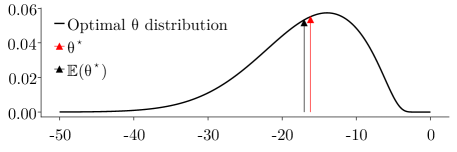
Figure 1: The optimal control parameter distribution given that the system parameter $p$ is normally distributed with mean $\hat{p}=5$ and $\sigma_{p}=5$. The red and black arrows respectively indicate the optimal control parameter without considering the randomness of $p$, and the expected value of the optimal control parameter distribution.

In order to derive some quantitative results, let us assign some numerical values to the parameters that define the optimal cost function $(q,r)=(100,1)$, our best guess $\hat{p}=5$ of the system parameter $p$ and its standard deviation $\sigma_{p}=5$. The optimal control parameter and cost derived for this system whose model is assumed to be known perfectly are given by $\hat{\theta}^{\star}=-16.180$ with the corresponding estimated cost $\hat{\mathcal{J}}^{\star}=8.090$. This deterministic performance estimate turns out to be overconfident when uncertainties in the system parameter are present. For example, if the prior knowledge on the distribution of the system parameter $p$ is utilized, the expected value of the controller parameter is found as $\mathbb{E}[\theta^{\star}]=-17.046$ and the corresponding expected cost is $\mathbb{E}[\mathcal{J}]=8.523$. The controller from the deterministic training/optimization is not only overconfident about its performance; but also is less robust against modeling errors, as the Bayesian learning yields a closed-loop stable system for a wider range of values of $p$.

Finally, Figure 1 shows the optimal control parameter distribution given that the system parameter $p$ is normally distributed with mean $\hat{p}=5$, standard deviation $\sigma_{p}=5$. This figure also shows the mean values of the optimal control distribution with the black arrow and the optimal control parameter a deterministic approach would yield in red. We notice that the Bayesian learning that yields the optimal control parameter distribution is more concerned about system stability due to the uncertainty in the parameter $p$, a feat that the deterministic training may not reason about.

2.2 Optimal Control under Parameter Uncertainty and Measurement Noise

Consider the scenario in which the system (1) is also subject to measurement errors; that is, our measurement model for the state $x$ is probabilistic and is distributed according to the Gaussian $\mathcal{N}(x,\sigma^{2})$. Since the controller uses this measurement to determine its action, the closed-loop system has to be modelled as a stochastic differential equation (SDE), given by

$$\begin{cases}dx(t)=(p+\theta)x(t)\,dt+\theta\sigma\,dW_{t},\\ x(0)=1,\end{cases}$$ (5)

where $W$ denotes the Wiener process [14]. The initial state is assumed deterministic and is set to unity for simplicity. The unique solution to this SDE is given by

$$x(t)=e^{(p+\theta)t}+\theta\sigma\int_{0}^{t}e^{(p+\theta)(t-s)}dW_{s}.$$ (6)

Lemma 1

The conditional expectation $\mathbb{E}\left[\mathcal{J}\mid p\right]$ of the performance index (2) given the system parameter $p$ is

$$\mathbb{E}\left[\mathcal{J}\mid p\right] =-\frac{1}{4}\frac{q+r\theta^{2}}{p+\theta}\left[\theta^{2}\sigma^{2}T+\left(1-e^{2T(p+\theta)}\right)\left(1+\frac{1}{2}\frac{\theta^{2}\sigma^{2}}{p+\theta}\right)\right].$$

Proof 1

Substituting the solution (6) of the SDE (5) expression into the performance measure (2) yields

$$\mathcal{J}= -\frac{1}{4}\frac{q+r\theta^{2}}{p+\theta}\left(1+e^{2T(p+\theta)}\right)+(q+r\theta^{2})\theta\sigma\int_{0}^{T}e^{(p+\theta)t}\int_{0}^{t}e^{(p+\theta)(t-s)}dW_{s}dt\;+$$

$$\hskip 14.22636pt\frac{1}{2}(q+r\theta^{2})\theta^{2}\sigma^{2}\int_{0}^{T}\left(\int_{0}^{t}e^{(p+\theta)(t-s)}dW_{s}\right)^{2}dt$$

The conditional expectation of this quantity given the system parameter $p$ under the distribution induced by the Wiener process may be computed in closed-form using Itô calculus:

$$\mathbb{E}_{W}\left[\mathcal{J}\mid p\right] =-\frac{1}{4}\frac{q+r\theta^{2}}{p+\theta}\left(1-e^{2T(p+\theta)}\right)+(q+r\theta^{2})\theta\sigma\int_{0}^{T}e^{(p+\theta)t}\cancelto{0}{\mathbb{E}_{W}\left[\int_{0}^{t}e^{(p+\theta)(t-s)}dW_{s}~{}\Big{\rvert}p\right]}dt+$$

$$\hskip 14.22636pt\frac{1}{2}(q+r\theta)^{2}\theta^{2}\sigma^{2}\int_{0}^{T}\mathbb{E}_{W}\left[\left(\int_{0}^{t}e^{(p+\theta)(t-s)}dW_{s}\right)^{2}~{}\bigg{\rvert}p\right]dt$$

$$=-\frac{1}{4}\frac{q+r\theta^{2}}{p+\theta}\left(1-e^{2T(p+\theta)}\right)+\frac{1}{2}(q+r\theta^{2})\theta^{2}\sigma^{2}\int_{0}^{T}\left(\int_{0}^{t}e^{2(p+\theta)(t-s)}ds\right)dt$$

$$=-\frac{1}{4}\frac{q+r\theta^{2}}{p+\theta}\left(1-e^{2T(p+\theta)}\right)+\frac{1}{2}(q+r\theta^{2})\theta^{2}\sigma^{2}\int_{0}^{T}-\frac{1}{2(p+\theta)}\left(1-e^{2T(p+\theta)}\right)dt$$

$$=-\frac{1}{4}\frac{q+r\theta^{2}}{p+\theta}\left[\theta^{2}\sigma^{2}T+\left(1-e^{2T(p+\theta)}\right)\left(1+\frac{1}{2}\frac{\theta^{2}\sigma^{2}}{p+\theta}\right)\right]. \blacksquare$$

It is easily shown that this quantity is positive for all $T>0$. Furthermore, it blows up as the horizon $T$ is extended to infinity. This is not surprising since a nonzero measurement noise causes the state to oscillate around the origin, rather than asymptotically converging to it, incurring nonzero cost all the while.

We have kept the system parameter $p$ constant in this analysis so far. Uncertainty over this variable can be incorporated by taking a further expectation

$$\mathbb{E}[\mathcal{J}]:=\mathbb{E}_{p}\left[\mathbb{E}_{W}\left[\mathcal{J}\mid p\right]\right],$$

of $\mathbb{E}_{W}\left[\mathcal{J}\mid p\right]$ over $p$, which must be accomplished numerically as it does not admit a closed-form expression.

We can then minimize $\mathbb{E}[\mathcal{J}]$ over the control parameter in order to study the effects of both kinds of uncertainties on the optimal controller. Such a study is provided in Figures 3 and 3, where we have plotted the optimal control parameter $\theta^{\star}$ and the minimal expected cost $\mathbb{E}[\mathcal{J}]$ as a function of the standard deviations of the measurement noise $\sigma$ and the system parameter $\sigma_{p}$. The constants we used to generate the data are given by $q=r=1$ and $T=\hat{p}=3$. Our first observation is that the magnitude of the optimal control parameter is an increasing function of system parameter uncertainty and a decreasing function of measurement uncertainty. Our second observation is that if the measurement noise is small, then the optimal control parameter is insensitive to system parameter uncertainty as long as this uncertainty is small. The optimal cost shares this insensitivity for an even wider range of values of $\sigma_{p}$. In a similar vein, if the uncertainty in the system parameter is large, then the optimal control parameter is insensitive to the magnitude of the measurement noise. However, the optimal cost is still sensitive to this quantity.

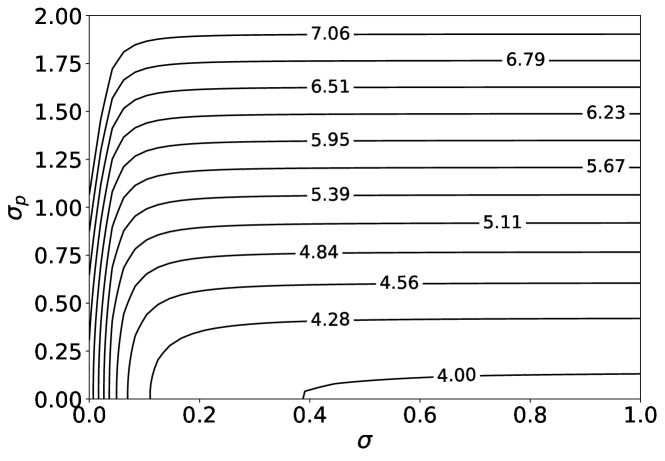
Figure 2: The optimal controller parameter magnitude $\left|{\theta^{\star}}\right|$.

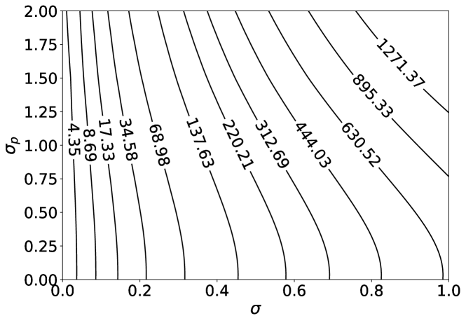
Figure 3: The minimal expected cost $\mathbb{E}[\mathcal{J}]$.

Key Takeaways

There are several advantages, to be inferred from the analyses in this section, of employing Bayesian learning to find the optimal control parameter $\theta$. Note that the optimal control parameter and cost derived for this system whose model is assumed to be known perfectly without measurement noise are given by $\theta_{d}^{\star}=-6.162$ and $\mathcal{J}_{d}^{\star}:=\mathcal{J}(\theta_{d}^{\star})=3.081$. This deterministic performance estimate is greatly overconfident when uncertainties in the system parameter and measurement are present. For example, if $\sigma=\nicefrac{{1}}{{10}}$ and $\sigma_{p}=\nicefrac{{\hat{p}}}{{5}}=\nicefrac{{6}}{{10}}$ then the expected cost with this controller parameter is, in fact, $\mathbb{E}[\mathcal{J}]=14.907$ and the overconfidence is an increasing function of both kinds of uncertainties.

The deterministic optimal controller certainly yields a controller parameter $\theta_{d}^{\star}$ that yields a stable system for a range of values for the system parameter $p$. In the numerical example, even if our best belief $\hat{p}$ of $p$ is erroneous by $100\%$, this controller will stabilize the system assuming no measurement noise.

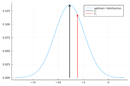
Figure 4: Laplace (Gaussian) approximation of the optimal control parameter distribution (shown in blue) given that the system parameter $p$ is distributed according to a truncated normal with mean $\hat{p}=3$ and $\sigma_{p}=2$ and bounds $(0,6)$. The deterministic optimal controller $\theta^{\star}_{d}$ is shown in black and the Bayesian solution $\theta^{\star}_{s}$ is shown in red.

However, consider the situation where we are pretty certain about the system parameter. Then, in the presence of measurement noise, this controller parameter induces a much larger expected cost than the optimal controller parameter, $\theta_{s}^{\star}$ that Bayesian learning yields (which has smaller magnitude, i.e., $\left|{\theta_{s}^{\star}}\right|<\left|{\theta_{d}^{\star}}\right|$). On the flip side, if the system parameter uncertainty is large, (e.g. $\sigma_{p}>\nicefrac{{\hat{p}}}{{2}}$), then, again, Bayesian learning is able to account for this fact to yield a controller parameter that is more robust. In this case, the situation is reversed and we find out $\left|{\theta_{d}^{\star}}\right|<\left|{\theta_{s}^{\star}}\right|$. Clearly, $\theta_{s}^{\star}$ stabilizes the system for a wider range of the true values of the system parameter than $\theta_{d}^{\star}$ does. When both measurement and system parameter uncertainties are present, Bayesian learning is able to precisely strike the trade-off between these competing uncertainties and yield controller parameter that results in a much better expected cost than a deterministic optimization does.

Finally, Figure 4 shows the Laplace (Gaussian) approximation to the optimal control parameter distribution given that the measurement noise has standard deviation $\sigma=\nicefrac{{1}}{{10}}$, and the system parameter $p$ is distributed according to a truncated normal with mean $\hat{p}=3$, standard deviation $\sigma_{p}=2$ and lower and upper bounds $(0,6)$. This figure also shows the mean values of the optimal control distribution with the black arrow and the optimal control parameter a deterministic approach would yield in red. We notice that the Bayesian learning that yields the optimal control parameter distribution is more concerned about system stability due to the uncertainty in the parameter $p$, a feat that the deterministic training may not reason about.

3 Conclusion

We solve the optimal control problem under the deterministic and Bayesian settings. The optimal control parameter changes sharply as a function of uncertainties in system parameters and measurements. This encourages the use of the Bayesian approach, which takes this variation into account, coming up with controllers that yield closed-loop stable systems for a wider range of system parameters. These findings motivate the use of Bayesian solutions to the control search problems, paving the way for the integration of Bayesian learning in data-driven control design techniques.

References

- [1] N. Heess, D. TB, S. Sriram, J. Lemmon, J. Merel, G. Wayne, Y. Tassa, T. Erez, Z. Wang, S. Eslami, et al., “Emergence of locomotion behaviours in rich environments,” arXiv preprint arXiv:1707.02286, 2017.
- [2] T. P. Lillicrap, J. J. Hunt, A. Pritzel, N. Heess, T. Erez, Y. Tassa, D. Silver, and D. Wierstra, “Continuous control with deep reinforcement learning,” arXiv preprint arXiv:1509.02971, 2015.
- [3] B. D. Argall, S. Chernova, M. Veloso, and B. Browning, “A survey of robot learning from demonstration,” Robotics and Autonomous Systems, vol. 57, no. 5, pp. 469–483, 2009.
- [4] M.-A. Beaudoin and B. Boulet, “Structured learning of safety guarantees for the control of uncertain dynamical systems,” arXiv preprint arXiv:2112.03347, 2021.
- [5] D. Sadigh and A. Kapoor, “Safe control under uncertainty,” arXiv preprint arXiv:1510.07313, 2015.
- [6] T. Shen, Y. Dong, D. He, and Y. Yuan, “Online identification of time-varying dynamical systems for industrial robots based on sparse bayesian learning,” Science China Technological Sciences, vol. 65, no. 2, pp. 386–395, 2022.
- [7] S. Linderman, M. Johnson, A. Miller, R. Adams, D. Blei, and L. Paninski, “Bayesian Learning and Inference in Recurrent Switching Linear Dynamical Systems,” in Proceedings of the 20th International Conference on Artificial Intelligence and Statistics, vol. 54, pp. 914–922, PMLR, 20–22 Apr 2017.
- [8] D. D. Fan, J. Nguyen, R. Thakker, N. Alatur, A.-a. Agha-mohammadi, and E. A. Theodorou, “Bayesian learning-based adaptive control for safety critical systems,” in 2020 IEEE international conference on robotics and automation (ICRA), pp. 4093–4099, IEEE, 2020.
- [9] K. P. Murphy, Machine learning: a probabilistic perspective. MIT press, 2012.
- [10] L. Cardelli, M. Kwiatkowska, L. Laurenti, and A. Patane, “Robustness guarantees for bayesian inference with gaussian processes,” in Proceedings of the AAAI Conference on Artificial Intelligence, vol. 33, pp. 7759–7768, 2019.
- [11] L. Cardelli, M. Kwiatkowska, L. Laurenti, N. Paoletti, A. Patane, and M. Wicker, “Statistical guarantees for the robustness of bayesian neural networks,” arXiv preprint arXiv:1903.01980, 2019.
- [12] M. Wicker, L. Laurenti, A. Patane, Z. Chen, Z. Zhang, and M. Kwiatkowska, “Bayesian inference with certifiable adversarial robustness,” in International Conference on Artificial Intelligence and Statistics, pp. 2431–2439, PMLR, 2021.
- [13] N. Ye and Z. Zhu, “Bayesian adversarial learning,” Advances in Neural Information Processing Systems, vol. 31, 2018.
- [14] L. C. Evans, An introduction to stochastic differential equations, vol. 82. American Mathematical Soc., 2012.