No-regret learning for repeated non-cooperative games with lossy bandits

Abstract

This paper considers no-regret learning for repeated continuous-kernel games with lossy bandit feedback. Since it is difficult to give the explicit model of the utility functions in dynamic environments, the players’ action can only be learned with bandit feedback. Moreover, because of unreliable communication channels or privacy protection, the bandit feedback may be lost or dropped at random. Therefore, we study the asynchronous online learning strategy of the players to adaptively adjust the next actions for minimizing the long-term regret loss. The paper provides a novel no-regret learning algorithm, called Online Gradient Descent with lossy bandits (OGD-lb). We first give the regret analysis for concave games with differentiable and Lipschitz utilities. Then we show that the action profile converges to a Nash equilibrium with probability 1 when the game is also strictly monotone. We further provide the mean square convergence rate $\mathcal{O}\left(k^{-2\min\{\beta,1/6\}}\right)$ when the game is $\beta-$strongly monotone. In addition, we extend the algorithm to the case when the loss probability of the bandit feedback is unknown, and prove its almost sure convergence to Nash equilibrium for strictly monotone games. Finally, we take the resource management in fog computing as an application example, and carry out numerical experiments to empirically demonstrate the algorithm performance.

1 Introduction

Online learning is an effective and necessary method for adaptive decision-making in dynamical or antagonistic environments. In this case, the agent usually needs to select an action without comprehensive models and then adapt to the next action based on the feedback information it receives. Such online learning methods are widely used as a central and canonical solution in various fields such as online recommendation [1], traffic routing [2], network resource allocation, and market prediction [3, 4, 5]. The online learning algorithms generally are designed to minimize the performance metric known as regret, which is the difference between the cumulative utility incurred by online decisions and that of the best-fixed decision in hindsight. A learning algorithm performs well if it meets the no-regret property, i.e., the increase of the regret is sublinear verse time [6, 7]. In other words, this property means that the average accumulated regret approaches zero asymptotically. A wide range of gradient-based no-regret learning algorithms has been established, e.g., online mirror descent [8, 9], exponential weights [10], follow-the-regularized-leader [11], online gradient descent [12, 13, 14], etc.

When a group of agents are interacting in a dynamic environment, each agent’s utility is not only influenced by its own action but also affected by the actions of its opponents. It is desirable that the self-interested agents can produce ideal collective behavior patterns by reaching equilibrium, and even obtain the best performance at the system level. Game theory provides tools and frameworks for the decision-making of non-cooperative agents (also called players). Algorithms for game equilibrium seeking have been studied by different methods such as the alternating direction method of multipliers [15, 16], the forward-backward operator splitting [17, 18, 19], discounted mirror descent [20], the iterative Tikhonov regularization [21], and average consensus protocol [22, 23], etc.

For the online decision-making with non-cooperative agents, the learning process can be modeled as playing repeated stage games among a group of players [24]. In addition, according to the different types of feedback information, numerous learning algorithms were developed respectively. In some situations, the gradient information or second-order Hessian of the player’s own utility function can be obtained after all nodes select actions, with which the next round action can be updated for maximizing its own utility. Since gradient feedback relies on full manipulation of its own utility function, it is called full-information. For this scenario, various convergence and regret analyses have been derived. For example, A no-regret algorithm is proposed in [25], which guarantees the convergence to the correlated equilibria in the repeated convex game. [26] focused on zero-sum games and showed that the actions of the players generated by a no-regret algorithm called NoRegretEgt converge to a min-max equilibrium. An adaptive regret-based learning procedure has been applied to track the correlated equilibria set of the congestion game [27]. When the gradient feedback is lost randomly, [28] focused on variationally stable games and showed that the online gradient descent algorithm converge almost surely to the set of Nash equilibria.

Nevertheless, in many practical problems, utility functions describing performances like service latency or reliability are difficult to model with explicit form in dynamic environments. Moreover, some low-power devices cannot run complicated models such as deep neural network to derive gradients. Besides, the player may not even be aware of the existence of its opponents. In these settings, the only information that the player can obtain after choosing an action is its utility value, which is known as bandit feedback. How to making online decision with such limited information is our concern.

With bandit feedback, players need to derive an individual gradient estimate from the utility value to update the next action. The most commonly used methods for gradient estimation can be divided into two types: multi-point estimation and single-point estimation. In fact, multi-point estimation techniques have been widely used in various optimization problems [29, 30, 31, 32, 33, 34], which are also known as zeroth-order oracles. Different from optimization, for the repeated game problem, each player’s utility is not only related to the actions taken by itself but also related to the actions taken by its opponents. When its actions change, the actions of its opponents will also change accordingly. Therefore, multi-point estimation methods are not applicable or cost too much, hence, single-point estimation methods such as simultaneous perturbation stochastic approximation (SPSA) [35, 36, 37, 38] are studied in the context of non-cooperative games. For example, the work of [39] considered potential games and proved that the exponential weight learning program with bandit feedback can achieve a sublinear expected regret and converge to Nash equilibrium. [40] showed that in monotone concave games, no-regret learning based on mirror descent with bandit feedback can converge to a Nash equilibrium with probability 1. With delayed bandit feedback in monotone games, [41] proposed an algorithm with sublinear regret and convergence to a Nash equilibrium. [42] showed that the no-regret learning in the Cournot game with bandit feedback can converge to the unique Nash equilibrium.

However, random loss and drop of the bandit feedback can occur in practical scenarios. Because the utility value evaluated by the external dynamic environment might be lost during transmission. Moreover, many computing architectures rely on the support of communication networks. Once the communication channel is interrupted, services and information feedback are dropped. Besides, device mobility can cause random variations in channel quality, aggravating communication channel failures [43]. In addition, to protect privacy or to perform intermittent queries to reduce the query costs, the bandit feedback can be actively dropped at random. Compounding bandit feedback with lossy feedback deserves in-depth studies, which is still lacking in the literature [6].

Consider fog computing as an application example, which is a distributed computing architecture for the Internet of Things (IoT). First of all, in the management of resources (including CPU time and storage) in fog computation, online learning for adaptive decision-making is an effective and necessary method. On the one hand, since the fog computing architecture targets at latency-sensitive IoT applications, real-time decision-making through online learning is an effective approach to improve user experience. On the other hand, the dynamic or noncooperative opponent IoT users are so complicated that we cannot build a comprehensive model. In this case, we adapt the decision through online learning with bandit feedback. Because the utility functions describing device latency and reliability in IoT are often difficult to establish explicitly, and low-power edge devices in fog computing cannot provide the computing power required for gradient computing. Adaptive online decision-making methods have also been highlighted in various problems of fog computing, eg, online computation scheduling [44], computation offloading [45], and resource allocation [13, 46]. An online bandit saddle-point (BanSaP) scheme for IoT management is developed in [47], which can achieve sublinear dynamic regret and can deal with time-varying constraints based on multi-point bandits.

Motivated by the above, we focus on no-regret learning with lossy bandits for repeated continuous-kernel games and take the resource management in fog computation as an application example. A preliminary version of the results was presented at the IEEE CDC in 2021 [48]. The current work makes several improvements and extensions compared to [48]: the major one we would like to emphasize is that we derive a convergence rate that can reach the same order of bandit feedback in [40] without information loss. In addition, we further relax the assumption to consider the case where the probability of bandit feedback loss is unknown. In this more practical and complex case, we demonstrate the convergence of the algorithm, for which the analysis is not intuitive. Furthermore, we take fog computation as an application example and carry out more simulations to discuss how loss probability influences the number of iterations and the times of updates required for the algorithm to reach a certain accuracy. The main contributions of our work are summarized as follows:

1. We propose a novel no-regret learning algorithm capable of online decision-making with lossy single-point bandit, called Online Gradient Descent with lossy bandits (OGD-lb).

2. We derive the expected regret bound of the learning algorithm, and show that it conforms to the no-regret property with concave utilities for proper step-sizes.

3. We show that OGD-lb converges to a Nash equilibrium with probability 1 for strictly monotone games, and it achieves $\mathcal{O}\left(k^{-2\min\{\beta,1/6\}}\right)$ convergence rate for $\beta-$strongly monotone games. It is worth noting that this convergence rate reaches the same order of bandit feedback in [40] without information loss.

4. We also consider the case when the probability of bandit feedback loss is unknown. The step-size is set by counting the number of players updates up to the current moment. We show that the algorithm still converges to a Nash equilibrium with probability 1 for strictly monotone games.

The paper is organized as follows. We state the problem formulation in Section 2 and introduce the algorithm in Section 3. The main results and proofs are provided in Sections 4 and 5, respectively. Section 6 presents simulation results. Some concluding remarks are provided in Section 7.

Notations: Denote $i\in\mathcal{N}=\{1,2,\dots,N\}$ as the player in the game, and $k=1,\dots,K$ as iterations. The indicator function of player $i$ at iteration $k$ is denoted by $I_{i}^{k}$. The $m$-dimensional real Euclidean space is denoted by $\mathbb{R}^{m}$. Sets are denoted by calligraphy, i.e., $\mathcal{A},\mathcal{B},\mathcal{C}$, etc. For a column vector $x\in\mathbb{R}^{m}$, $x^{\top}$ denotes its transpose $x^{\top}y=\left\langle x,y\right\rangle$ denotes the inner product of $x,y$, and the standard Euclidean norm is denoted by $\|x\|=\sqrt{x^{\top}x}$. Denote $\|x\|_{\infty}=\max_{1\leq i\leq N}|a_{i}|$ as the max norm. Use $P_{\mathcal{A}}(y)=\arg\min_{a\in\mathcal{A}}\|y-x\|$ to represent the projection of $y$ onto a closed convex set $\mathcal{A}$. For functions $f,\phi:\mathbb{R}\rightarrow\mathbb{R}^{+}$, we write $f(x)=\mathcal{O}(\phi(x))$ if $\lim\sup_{x\rightarrow\infty}\left|f(x)/\phi(x)\right|<\infty$, and $f(x)=o(\phi(x))$ if $\lim\sup_{k\rightarrow\infty}f(x)/\phi(x)=0$.

2 Problem formulation

In this section, a repeated concave game is formulated. Moreover, the definition of regret is introduced, which is a performance metric for the online learning algorithm.

2.1 Repeated Concave Games

The tuple $\mathcal{G}\equiv\mathcal{G}(\mathcal{N},\mathcal{A}\equiv\prod_{i=1}^{N}\mathcal{A}_{i},\left\{u_{i}\right\}_{i=1}^{N})$ denotes a utility maximization game, where $\mathcal{N}=\left\{1,\dots,N\right\}$ is the set of $N$ agents/players. $\mathcal{A}_{i}\subset\mathbb{R}^{d_{i}}$ is the action space of player $i$. And $u_{i}(a)=u_{i}(a_{i},a_{-i}):\mathcal{A}\rightarrow\mathbb{R}$ is player $i$’s utility function. Let $a_{-i}=(a_{1},\cdots,a_{i-1},a_{i+1},\cdots a_{N})$ and $\mathcal{A}_{-i}=\prod_{j\neq i}\mathcal{A}_{j}$ represent the actions and action space for all players except $i$, respectively. The action profile is denoted as $a=(a_{i},a_{-i})$. Our basic assumptions about the utility functions and the action sets are as follows.

Assumption 1.

For each player $i\in\mathcal{N}$,

1. the action set $\mathcal{A}_{i}$ is closed, convex, and compact with a nonempty interior.

2. $u_{i}(a_{i},a_{-i})$ is concave and continuously differentiable in $a_{i}\in\mathcal{A}_{i}$ for any given $a_{-i}\in\mathcal{A}_{-i}$;

3. $g_{i}(a_{i},a_{-i})=\nabla_{a_{i}}u_{i}\left(a_{i},a_{-i}\right)$ represents the partial gradient of $u_{i}(a_{i},a_{-i})$ with respect to $a_{i}$, which is $L_{i}$-Lipschitz continuous in $a\in\mathcal{A}$, i.e.,

   $$\left\|g_{i}\left(a\right)-g_{i}(a^{\prime})\right\|\leq L_{i}\left\|a-a^{\prime}\right\|,\quad\forall a,a^{\prime}\in\mathcal{A}.$$

Time is slotted as $k=1,2,\dots$, we assume that the players repeatedly play the game $\mathcal{G}(\mathcal{N},\mathcal{A}\equiv\prod_{i=1}^{N}\mathcal{A}_{i},\left\{u_{i}\right\}_{i=1}^{N})$. Each player $i$ sequentially chooses its action by learning from the available feedback information. The algorithm for adapting the player’s action is called “online learning”.

2.2 Regret of Online Learning Algorithm

Regret is usually taken as the metric to measure the performance of online learning algorithms. The learning protocol of a given repeated game is as follows: At iteration $k$, each player $i$ selects an action $a_{i,k}$ through a learning algorithm. Then the external environment such as the app user market evaluates the current action profile $(a_{i,k},a_{-i,k})$, and returns the value $u_{i}\left(a_{i,k},a_{-i,k}\right)$ to player $i$. The cumulative utility of player $i$ within $K$ iterations is denoted as $\sum_{k=1}^{K}u_{i}\left(a_{i,k},a_{-i,k}\right)$. To measure the performance of $\mathcal{A}$, the cumulative utility is usually compared with the utility obtained when a best-fixed decision in the hindsight is taken. The regret of node $i$ within $K$ iterations is formally defined as

$$\mathcal{R}eg^{(i)}\left(K\right)=\max_{a_{i}^{\prime}\in\mathcal{A}_{i}}\left\{\sum_{k=1}^{K}u_{i}\left(a_{i}^{\prime},a_{-i,k}\right)-\sum_{k=1}^{K}u_{i}\left(a_{i,k},a_{-i,k}\right)\right\}.$$

An online algorithm is no-regret if and only if the regret is sublinear as a function of time $K$, $\mathcal{R}eg^{(i)}(K)=o(K)$, i.e.,

$$\lim_{K\rightarrow\infty}\frac{\mathcal{R}eg^{(i)}(K)}{K}=0,\quad\forall i\in\mathcal{N}.$$ (1)

3 Online learning with lossy bandits

In this section, an online learning algorithm was designed, which is called Online Gradient Descent with lossy bandits (OGD-lb).

3.1 Lossy Bandits

With bandit feedback, the only information available to the players is the utility value with a given action. However, the utility value may not be available at each stage of online learning. Take the fog computation networks as an example, $a)$ the utility may be lost during transmission; $b)$ the interruption of network connection; $c)$ communication channel failures due to small-scale fading or IoT device mobility; $d)$ the player performs intermittent queries to reduce the query costs; $e)$ the player actively drops the utility for privacy protection, etc.

We consider the lossy bandits scenario as shown in Figure 1. At iteration $k$, each player $i\in\mathcal{N}$ submits its applied action $\hat{a}_{i,k}$ (obtained after perturbing intended action $a_{i,k}$) to the market. However, some players may not receive the utility value due to feedback loss, such as players 1 and 3 in Figure 1. Then the players that have received the utilities update their actions, while those that cannot receive the utility information keep their actions unchanged. For a detailed description of this process, please refer to the algorithm introduction in the next subsection.

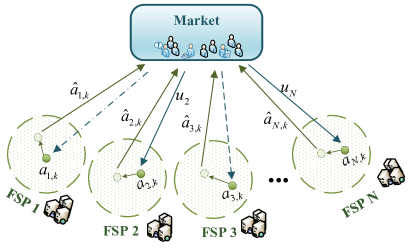
Figure 1: Lossy bandits (where FSP stands for fog service provider, the solid line represents the received information transmission, and the dashed line represents information loss; $a_{i,k}$ is the action of FSP $i$ at iteration $k$; $u_{i}$ is the utility value of FSP $i$).

Let $p_{i}$ denote the probability that player $i$ will receive its utility value, then the probability of information loss is $1-p_{i}$. Denote the indicator function as follows:

$$\begin{split}I_{i}^{k}=\left\{\begin{array}[]{lr}1,\;{\rm if\;the\;bandit\;is\;received;}\\ 0,\;{\rm if\;the\;bandit\;is\;lost.}\end{array}\right.\end{split}$$

Then $\mathbb{E}\left[I_{i}^{k}\right]=p_{i}>0$.

3.2 Learning Process

The learning process of our proposed algorithm can be divided into three parts. The first part is initializing parameters. The second part is estimating the gradient with bandit feedback, in which we use a one-point estimation method motivating by simultaneous perturbation stochastic approximation (SPSA) [35]. The third part is performing projected gradient descent.

At each stage, the players update their actions by the novel algorithm called Online Gradient Descent with lossy bandits (OGD-lb) (Algorithm 1), where the action of player $i$ at stage $k$ is denoted by $a_{i,k}$. A detailed description of the algorithm is shown below and the corresponding position with the pseudo-code is marked in parentheses.

• (Initialization) Set $k=1$, require step-size $\{\gamma_{i,k}\}>0$ and query radius $\{\delta_{k}\}>0$ are non-increasing sequences, choose an action $a_{i,k}\in\mathcal{A}_{i}$ for each player $i\in\mathcal{N}$.

• (Line 4-5) Fix a $\delta_{k}>0$ and select a vector $\lambda_{i,k}$ from the unit sphere $\mathbb{S}_{i}\equiv\mathbb{S}^{d_{i}}\subset\mathbb{R}^{d_{i}}$ that is independent with each other at stage $k$. To ensure that the perturbed point is still in the action space $\mathcal{A}_{i}$, we select an interior point $c_{i}$ from $\mathcal{A}_{i}$ and let $\mathbb{B}_{r_{i}}\left(c_{i}\right)$ be a $r_{i}$-ball centered at $c_{i}\in\mathcal{A}_{i}$ so that $\mathbb{B}_{r_{i}}\left(c_{i}\right)\subseteq\mathcal{A}_{i}$. We then take

  $$\theta_{i,k}=\lambda_{i,k}-r_{i}^{-1}\left(a_{i,k}-c_{i}\right)$$ (2)

  as the perturbation direction.

• (Line 6) Get an applied action $\hat{a}_{i,k}=a_{i,k}+\delta_{k}\theta_{i,k}=a_{i,k}^{\delta_{k}}+\delta_{k}\lambda_{i,k}$ to play, where

  $$a_{i,k}^{\delta_{k}}=a_{i,k}-r_{i}^{-1}\delta_{k}\left(a_{i,k}-c_{i}\right)$$ (3)

  with $\delta_{k}/r_{i}<1$. Note that it is equivalent to first moving each intended action $a_{i,k}$ to $a_{i,k}^{\delta_{k}}$, and then perturbing along the direction $\lambda_{i,k}$ to get the applied action $\hat{a}_{i,k}$.

• (Line 7-8) After that, we obtain the utility value $\hat{u}_{i,k}=u_{i}\left(\hat{a}_{i,k},\hat{a}_{-i,k}\right)$, and derive an estimated gradient by

  $$\hat{g}_{i,k}\left({a}_{i,k},{a}_{-i,k}\right)=\frac{d_{i}}{\delta_{k}}\hat{u}_{i,k}\lambda_{i,k}.$$ (4)

• (Line 9) Finally, if $I_{i}^{k}=1$, player $i$ updates its action $a_{i,k+1}$ by the projected gradient method. Otherwise, $a_{i,k}$ remains unchanged.

In summary, we provide a novel algorithm OGD-lb, for which the pseudo-code is shown in Algorithm 1. For convenience, we abbreviate $\hat{g}_{i}\left({x}_{i,k},{x}_{-i,k}\right)$ as $\hat{g}_{i,k}$ in the rest.

Algorithm 1 OGD-lb

Require: step-size $\{\gamma_{i,k}\}>0$, query radius $\{\delta_{k}\}>0$, safety ball $\mathbb{B}_{r_{i}}\left(c_{i}\right)\subseteq\mathcal{A}_{i}$
1: choose $a_{i,k}\in\mathcal{A}_{i}$, iteration $k\leftarrow 1$
2: repeat
3:  for each player $i$ do
4:   draw $\lambda_{i,k}$ uniformly from $S_{i}\equiv S^{d_{i}}$ of $\mathbb{R}^{d_{i}}$
5:   set $\theta_{i,k}\leftarrow\lambda_{i,k}-r_{i}^{-1}(a_{i,k}-c_{i})$
6:   play $\hat{a}_{i,k}\leftarrow a_{i,k}+\delta_{k}\theta_{i,k}$
7:   receive $\hat{u}_{i,k}=u_{i}\left(\hat{a}_{i,k},\hat{a}_{-i,k}\right)$
8:   set $\hat{g}_{i,k}\leftarrow\left(d_{i}/\delta_{k}\right)\hat{u}_{i,k}\lambda_{i,k}$
9:   update

$$\quad\quad\quad a_{i,k+1}\leftarrow\left\{\begin{array}[]{ll}P_{\mathcal{A}_{i}}\left(a_{i,k}+\gamma_{i,k}\hat{g}_{i,k}\right),&\text{ if }I_{i}^{k}=1\\ a_{i,k},&\text{ if }I_{i}^{k}=0\end{array}\right.$$

10:  end for
11:  $k\leftarrow k+1$
12: until end

With respect to the independence of the perturbation sequences $\{\lambda_{i,k}\}$ and the indicator functions $\{I_{i}^{k}\}$ used in Algorithm 1, the following assumption is made.

Assumption 2.

At each stage $k$, the random variables $\lambda_{i,k},I_{i}^{k},i=1,\cdots,N$ are mutually independent. In addition, for each $i\in\mathcal{N}$, $\{I_{i}^{k}\}_{k\geq 1}$ are independent and identically distributed (i.i.d.) across time steps.

4 Main Results

In this section, the main theoretical results are given, which contain the expected regret bound, convergence, and convergence rate with different algorithm step-size selections.

4.1 Regret Analysis

Here, we demonstrate the expected regret bound of Algorithm 1 and show that it meets no-regret property. For detailed proofs of Theorem 1 and Corollary 1, please refer to Section5.2 and 5.3.

Theorem 1 (Regret bound in expectation).

Let Assumptions 1-2 hold. Consider the players follow Algorithm 1 with step-size $\gamma_{i,k}=\gamma_{k}p_{i}^{-w}$ and constant $w>0$. Suppose that $\{\gamma_{k}\}$ and $\{\delta_{k}\}$ are non-increasing sequences with $\delta_{1}<\min_{i}r_{i}$. Then for each $i\in\mathcal{N}$,

$$\mathbb{E}\left[\mathcal{R}eg^{(i)}(K)\right] \leq\frac{p_{i}^{w-1}B_{i}^{2}}{2\gamma_{K}}+\sum_{k=1}^{K}B_{i}L_{i}\sqrt{N}\delta_{k}$$

$$+\sum_{k=1}^{K}\frac{p_{i}^{w-1}}{2\gamma_{k}}\frac{G_{i}^{2}}{\delta_{k}^{2}}\mathbb{E}\left[\gamma_{i,k}^{2}\right],$$ (5)

where $B_{i}=\max_{a_{i}^{\prime},a_{i}\in\mathcal{A}_{i}}\|a_{i}^{\prime}-a_{i}\|$ represents the Euclidean diameter of $\mathcal{A}_{i}$, and $G_{i}^{2}=d_{i}^{2}\max_{a\in\mathcal{A}}\left|u_{i}(a_{i},a_{-i})\right|^{2}$ is a bounded constant.

Theorem 1 proves that the number of players $N$, and the algorithm update parameters (step-size $\gamma_{i,k}$ and perturbation radius $\delta_{k}$) of player $i\in\mathcal{N}$ at iteration $k$ all affect the expectation-valued regret bound of the Algorithm 1. Then, for some specific step sizes, the no-regret property is proved in the following corollary.

Corollary 1 (Expected No-regret).

Suppose Assumptions 1-2 hold. Consider the players follow Algorithm 1 with $\gamma_{i,k}=1/(k^{b}p_{i})$ and $\delta_{k}={\delta_{1}}k^{-c}$ with $0<b<1$, $0<c<b/2$ and $\delta_{1}<\min_{i}r_{i}$. Then for each $i\in\mathcal{N}$,

$$\mathbb{E} \left[\mathcal{R}eg^{(i)}(K)\right]\leq\frac{B_{i}^{2}}{2}k^{b}+\frac{B_{i}L_{i}\sqrt{N}{\delta_{1}}}{1-c}K^{1-c}$$

$$\quad+\frac{G_{i}^{2}}{2p_{i}^{2}{\delta_{1}^{2}}(1-b+2c)}K^{1-b+2c}+B_{i}L_{i}\sqrt{N}{\delta_{1}}+\frac{G_{i}^{2}}{2p_{i}^{2}{\delta_{1}^{2}}}.$$

Remark 1.

According to Corollary 1, we obtain that

$$\mathbb{E}\left[\mathcal{R}eg^{(i)}(K)\right]=\mathcal{O}(K^{\max\{b,1-c,1-b+2c\}}).$$

Thus, $\lim\sup_{K\rightarrow\infty}\mathbb{E}\left[\mathcal{R}eg^{(i)}(K)\right]/K=0,$ which implies that Algorithm 1 is no-regret. Note that it is desirable for the players to follow a no-regret learning algorithm because everyone wishes that the online strategy he adopted is at least not worse than any static strategy. For example, a regret bound $K^{3/4}$ can be obtained with $b=3/4$ and $c=1/4$, which is a common bound in the online learning literature, such as [37].

4.2 Convergence Analysis

Definition 1.

(Nash equilibrium). The profile $a^{*}\in\mathcal{A}$ is a Nash equilibrium for a given game $\mathcal{G}$ if for each $i\in\mathcal{N}$,

$$u_{i}\left(a_{i}^{*},a_{-i}^{*}\right)\geq u_{i}\left(a_{i},a_{-i}^{*}\right),\quad\forall a_{i}\in\mathcal{A}_{i}.$$

It is worth noting that a no-regret algorithm cannot ensure the convergence to the Nash equilibrium in general, for instance, the sequence of actions can converge to the coarsest equilibrium or correlated equilibrium [24]. Convergence to a Nash equilibrium is “considerably more difficult” because Nash equilibrium is a more stable equilibrium. To study the convergence of the algorithm, we further restrict the game structure to a strictly monotone game [49]. In the following, the pseudo-gradient mapping is denoted by $g(a)=(g_{1}(a_{1},a_{-1}),\dots,g_{N}(a_{N},a_{-N}))^{\top}$.

Assumption 3.

Suppose that $\mathcal{G}$ is a strictly monotone game on action space $\mathcal{A}$, i.e.,

$$\left\langle g(a)-g(a^{\prime}),a-a^{\prime}\right\rangle<0,\quad\forall a,a^{\prime}\in\mathcal{A},a\neq a^{\prime}.$$

Remark 2.

When the action set $\mathcal{A}_{i}$ is convex and compact for each player $i\in\mathcal{N}$, a strictly monotone game admits a unique Nash equilibrium $a^{*}$, which is equivalent to the solution of the variational inequality[50]

$$\sum_{i\in\mathcal{N}}\left\langle g_{i}\left(a_{i}^{*},a_{-i}^{*}\right),a_{i}-a_{i}^{*}\right\rangle\leq 0,\quad\forall a_{i}\in\mathcal{A}_{i}.$$ (6)

The assumption regarding the step-size is as follows, which can also be found in the existing literature, see e.g., [40].

Assumption 4.

For each $i\in\mathcal{N}$, the sequences $\{\gamma_{k}\}$ and perturbation radius $\{\delta_{k}\}$ satisfy $\delta_{1}<\min_{i}r_{i}$, and

$$\lim_{k\rightarrow\infty}\gamma_{k}=\lim_{k\rightarrow\infty}\delta_{k}=0,\quad\sum_{k=1}^{\infty}\gamma_{k}=\infty,$$

$$\sum_{k=1}^{\infty}\gamma_{k}\delta_{k}<\infty,\quad\sum_{k=1}^{\infty}\frac{\gamma_{k}^{2}}{\delta_{k}^{2}}<\infty.$$

Then, we can obtain the convergence of the algorithm.

Theorem 2 (Almost sure convergence).

Consider Algorithm 1 with $\gamma_{i,k}=\gamma_{k}p_{i}^{-1}$ for all $i\in\mathcal{N}$. Let Assumptions 1-4 hold. Then the action sequence $\hat{a}_{k}$ converges to a Nash equilibrium with probability 1.

The results are proved as follows. Firstly, with Assumptions 1-3, we prove that $D\left(a_{k},a^{*}\right)=\|a_{k}-a^{*}\|^{2}/2$ converges almost surely (a.s.) to a finite random variable $D_{\infty}$. We then prove that there exists a subsequence $\{a_{k_{r}}\}$ of $\{a_{k}\}$ which converges a.s. to the Nash equilibrium. Finally, combining the above two results, we prove Theorem 2. Please refer to Section 5.4 for detailed proofs.

4.3 Rate Analysis

In order to study the convergence rate of the proposed algorithm, we further strengthen the game structure into a $\beta$-strongly monotone game with specific step-sizes. For the detailed proof of Theorem 3, please refer to Section 5.5.

Assumption 5.

Suppose that $\mathcal{G}$ is a $\beta-$strongly monotone game on action space $\mathcal{A}$, i.e.,

$$\left\langle g\left(a\right)-g(a^{\prime}),a-a^{\prime}\right\rangle\leq-\beta\|a-a^{\prime}\|^{2},\quad\forall a,a^{\prime}\in\mathcal{A}.$$

Theorem 3 (Convergence rate in a mean-squared sense).

Suppose Assumptions 1, 2, and 5 hold. Consider the players follow Algorithm 1 with $\gamma_{i,k}={1}/({kp_{i}})$ and $\delta_{k}={\delta_{1}}k^{-1/3}$ with $\delta_{1}<\min_{i}r_{i}$. Then

$$\mathbb{E}\left[\|\hat{a}_{k}-a^{*}\|^{2}\right]=\mathcal{O}\left(k^{-2\min\{\beta,1/6\}}\right).$$

4.4 Convergence with Unknown Lossy Probability

In addition, we consider the scenario where $p_{i}$ is unknown. Let the step-size be a function related to the number of updates up to the current time $k$, i.e., step-size $\gamma_{i,k}={1}/{(\Gamma_{i}^{k})^{q}}$ where $\Gamma_{i}^{k}=\sum_{t=1}^{k}I_{i}^{t}$, $q\in(1/2,1]$, and $\mathbb{E}[I_{i}^{k}]=p_{i}>0$ for all $i$ and $k$. In this setting, the symbol $p_{i}$ is only used for analysis.

Then, we can obtain the convergence of the algorithm when the loss probability is unknown in advance, for which the proof can be found in Section 5.6.

Theorem 4 (Almost sure convergence with unknown $p_{i}$).

Suppose Assumptions 1, 2, and 3 hold. Consider the players follow Algorithm 1, where $\gamma_{i,k}={1}/{(\Gamma_{i}^{k})^{q}}$ with $\Gamma_{i}^{k}=\sum_{t=1}^{k}I_{i}^{t}$ and $q\in(1/2,1]$, and the perturbation radius $\{\delta_{k}\}$ satisfies $\delta_{1}<\min_{i}r_{i}$, and

$$\lim_{k\rightarrow\infty}\delta_{k}=0,~{}\sum_{k=1}^{\infty}k^{-q}\delta_{k}<\infty,~{}\sum_{k=1}^{\infty}k^{-2q}\delta_{k}^{-2}<\infty.$$ (7)

Then the sequence of realized actions $\hat{a}_{k}$ converges to the Nash equilibrium with probability 1.

5 Proof of Main Results

In this part, we provide detailed proofs corresponding to the main results established in Section 4.

5.1 Preliminary Analysis

Let $\mathcal{F}_{k}$ be a $\sigma-$algebra of random variables up to stage $k$, i.e., $\mathcal{F}_{k}\triangleq\sigma\left\{a_{i,1},\lambda_{i,s},I_{i}^{s},i\in\mathcal{N},1\leq s\leq k-1\right\}$. We denote

$$\hat{g}_{i,k}=g_{i}\left(a_{k}\right)+\rho_{i,k+1}+\zeta_{i,k}$$ (8)

where

$$\rho_{i,k+1}=\hat{g}_{i,k}-\mathbb{E}\left[\hat{g}_{i,k}\mid\mathcal{F}_{k}\right],$$ (9)

$$\zeta_{i,k}=\mathbb{E}\left[\hat{g}_{i,k}\mid\mathcal{F}_{k}\right]-g_{i}\left(a_{k}\right)$$ (10)

are noise term and systematic bias respectively. Then, a lemma of SPSA estimator is introduced as follows.

Lemma 5.

[40, Lemma 4] Let Assumption 1 holds. Then the SPSA estimator $(\hat{g}_{i,k})_{i\in\mathcal{N}}$ satisfies

$$\mathbb{E}\left[\hat{g}_{i,k}\mid\mathcal{F}_{k}\right]=g_{i,k}^{\delta_{k}}=\nabla_{a_{i,k}^{\delta_{k}}}u_{i}^{\delta_{k}}(a_{i,k}^{\delta_{k}},a_{-i,k}^{\delta_{k}}),$$ (11)

where $u_{i}^{\delta_{k}}(a_{i,k}^{\delta_{k}},a_{-i,k}^{\delta_{k}})$ is a $\delta$-smooth utility function and $a_{i,k}^{\delta_{k}}$ is defined in equation (3). In addition, we have

$$\|\zeta_{i,k}\|\leq L_{i}\sqrt{N}\delta_{k}$$ (12)

and the second moment of the noise term $\rho_{i,k+1}$ is $\mathcal{O}\left(1/\delta_{k}^{2}\right).$

Remark 3.

When the perturbation radius $\delta_{k}\rightarrow 0,$ the bias will decrease to zero, but the noise will increase to infinity. Therefore, there is a bias-variance tradeoff between the bias and noise variance. Thus, the perturbation radius $\delta_{k}$ should be selected carefully.

In the following, we present a preliminary lemma that will be used for convergence analysis.

Lemma 6.

Suppose Assumptions 1-3 hold. Define $D_{k}=\sum_{i\in\mathcal{N}}p_{i}^{w-1}D_{i,k}$ with $D_{i,k}=\frac{1}{2}\|a_{i,k}-a_{i}^{\prime}\|^{2}$ for $a_{i}^{\prime}\in\mathcal{A}_{i}$, and $\tilde{\gamma}_{i,k}=\gamma_{i,k}-\gamma_{k}p_{i}^{-w}$ with a constant $w>0$. Then

$$\mathbb{E}\left[D_{k+1}\mid\mathcal{F}_{k}\right] \leq D_{k}+\gamma_{k}{\left\langle g(a^{{}^{\prime}}),a_{k}-a^{{}^{\prime}}\right\rangle}+\sum_{i\in\mathcal{N}}B_{i}L_{i}\sqrt{N}\gamma_{k}\delta_{k}$$

$$+\sum_{i\in\mathcal{N}}({C_{i}}+B_{i}L_{i}\sqrt{N}\delta_{k})p_{i}^{w-1}\mathbb{E}\left[\left|\tilde{\gamma}_{i,k}\right|\mid\mathcal{F}_{k}\right]$$

$$+\sum_{i\in\mathcal{N}}\frac{G_{i}^{2}p_{i}^{w-1}}{2\delta_{k}^{2}}\mathbb{E}\left[\gamma_{i,k}^{2}\mid\mathcal{F}_{k}\right],\quad{\forall a^{{}^{\prime}}\in\mathcal{A}},$$

where ${C_{i}}$ is some scalar satisfying $\left|\left\langle g_{i}(a),a_{i}-a_{i}^{\prime}\right\rangle\right|\leq{C_{i}}$ for any $a\in\mathcal{A}$ and $a_{i}^{\prime}\in\mathcal{A}_{i}$ , $B_{i}=\max_{a_{i}^{\prime},a_{i}\in\mathcal{A}_{i}}\|a_{i}^{\prime}-a_{i}\|$ is the Euclidean diameter of $\mathcal{A}_{i}$, $L_{i}$ denotes the Lipschitz constant and $G_{i}^{2}=d_{i}^{2}\max_{a\in\mathcal{A}}\left|u_{i}(a_{i},a_{-i})\right|^{2}$ is a bounded constant.

Proof.

Note by Algorithm 1 and the definition of $\sigma-$algebra that $a_{k}$ is adapted to $\mathcal{F}_{k}$. Since $\rho_{i,k+1}$ is an $\mathcal{F}_{k}-$adapted martingale difference sequence by (9), we have that

$$D_{i,k+1} =D(a_{i,k+1},a_{i}^{\prime})$$

$$=\frac{1}{2}\|a_{i,k+1}-a_{i}^{\prime}\|^{2}\mathbf{1}_{\left\{I_{i}^{k}=1\right\}}+\frac{1}{2}\|a_{i,k}-a_{i}^{\prime}\|^{2}\mathbf{1}_{\left\{I_{i}^{k}=0\right\}}$$

$$\overset{(a)}{\leq}\left(\frac{1}{2}\|a_{i,k}+\gamma_{i,k}\hat{g}_{i,k}-a_{i}^{\prime}\|^{2}\right)\mathbf{1}_{\left\{I_{i}^{k}=1\right\}}$$

$$\quad\quad+\frac{1}{2}\|a_{i,k}-a_{i}^{\prime}\|^{2}\mathbf{1}_{\left\{I_{i}^{k}=0\right\}}$$

$$=\left(\frac{1}{2}\|a_{i,k}-a_{i}^{\prime}\|^{2}+\gamma_{i,k}\left\langle\hat{g}_{i,k},a_{i,k}-a_{i}^{\prime}\right\rangle+\frac{1}{2}\gamma_{i,k}^{2}\|\hat{g}_{i,k}\|^{2}\right)$$

$$\quad\quad\mathbf{1}_{\left\{I_{i}^{k}=1\right\}}+\frac{1}{2}\|a_{i,k}-a_{i}^{\prime}\|^{2}\mathbf{1}_{\left\{I_{i}^{k}=0\right\}}$$

$$\overset{{\eqref{es}}}{=}D_{i,k}+\left(\gamma_{i,k}\left\langle g_{i}(a_{k})+\rho_{i,k+1}+\zeta_{i,k},a_{i,k}-a_{i}^{\prime}\right\rangle\right)\mathbf{1}_{\left\{I_{i}^{k}=1\right\}}$$

$$\quad\quad+\frac{1}{2}\gamma_{i,k}^{2}\|\hat{g}_{i,k}\|^{2}\mathbf{1}_{\left\{I_{i}^{k}=1\right\}},\quad{\forall a_{i}^{{}^{\prime}}\in\mathcal{A}_{i},}$$ (13)

where $(a)$ comes from the nonexpansibility of the projection.

Let $G_{i}^{2}=d_{i}^{2}\max_{a\in\mathcal{A}}|u_{i}(a_{i},a_{-i})|^{2}$, and we can know that $G_{i}$ is a bounded constant because the set $\mathcal{A}$ is compact and the function $u_{i}$ is continuous (Assumption 1). Thus, with Line 8 of Algorithm 1, we obtain $\|\hat{g}_{i,k}\|^{2}\leq G_{i}^{2}/\delta_{k}^{2},$ and inequality (5.1) becomes

$$D_{i,k+1} \leq D_{i,k}+(\gamma_{i,k}\left\langle g_{i}(a_{k}),a_{i,k}-a_{i}^{\prime}\right\rangle)\mathbf{1}_{\left\{I_{i}^{k}=1\right\}}$$

$$+(\gamma_{i,k}\left\langle\rho_{i,k+1},a_{i,k}-a_{i}^{\prime}\right\rangle)\mathbf{1}_{\left\{I_{i}^{k}=1\right\}}$$

$$+(\gamma_{i,k}\left\langle\zeta_{i,k},a_{i,k}-a_{i}^{\prime}\right\rangle)\mathbf{1}_{\left\{I_{i}^{k}=1\right\}}$$

$$+\frac{1}{2}\gamma_{i,k}^{2}\frac{G_{i}^{2}}{\delta_{k}^{2}}\mathbf{1}_{\left\{I_{i}^{k}=1\right\}}.$$ (14)

Expressing $\gamma_{i,k}=\gamma_{k}p_{i}^{-w}+\tilde{\gamma}_{i,k}$ with $\tilde{\gamma}_{i,k}=\gamma_{i,k}-\gamma_{k}p_{i}^{-w}$, we have

$$D_{i,k+1}\leq D_{i,k}+\left[\tilde{\gamma}_{i,k}\left\langle g_{i}(a_{k}),a_{i,k}-a_{i}^{\prime}\right\rangle\right]\mathbf{1}_{\left\{I_{i}^{k}=1\right\}}$$

$$+\left[\tilde{\gamma}_{i,k}\left\langle\rho_{i,k+1},a_{i,k}-a_{i}^{\prime}\right\rangle\right]\mathbf{1}_{\left\{I_{i}^{k}=1\right\}}+\left[\tilde{\gamma}_{i,k}\left\langle\zeta_{i,k},a_{i,k}-a_{i}^{\prime}\right\rangle\right]\mathbf{1}_{\left\{I_{i}^{k}=1\right\}}$$

$$+\frac{\gamma_{k}}{p_{i}^{w}}\left\langle g_{i}(a_{k}),a_{i,k}-a_{i}^{\prime}\right\rangle\mathbf{1}_{\left\{I_{i}^{k}=1\right\}}+\frac{\gamma_{k}}{p_{i}^{w}}\left\langle\rho_{i,k+1},a_{i,k}-a_{i}^{\prime}\right\rangle\mathbf{1}_{\left\{I_{i}^{k}=1\right\}}$$

$$+\frac{\gamma_{k}}{p_{i}^{w}}\left\langle\zeta_{i,k},a_{i,k}-a_{i}^{\prime}\right\rangle\mathbf{1}_{\left\{I_{i}^{k}=1\right\}}+\frac{1}{2}\gamma_{i,k}^{2}\frac{G_{i}^{2}}{\delta_{k}^{2}}\mathbf{1}_{\left\{I_{i}^{k}=1\right\}}$$

$$\leq D_{i,k}+\left[\left|\tilde{\gamma}_{i,k}\right|\left|\left\langle g_{i}(a_{k}),a_{i,k}-a_{i}^{\prime}\right\rangle\right|\right]\mathbf{1}_{\left\{I_{i}^{k}=1\right\}}$$

$$+\left[\left(\tilde{\gamma}_{i,k}\right)\left\langle\rho_{i,k+1},a_{i,k}-a_{i}^{\prime}\right\rangle\right]\mathbf{1}_{\left\{I_{i}^{k}=1\right\}}$$

$$+\left[\left|\tilde{\gamma}_{i,k}\right|\left|\left\langle\zeta_{i,k},a_{i,k}-a_{i}^{\prime}\right\rangle\right|\right]\mathbf{1}_{\left\{I_{i}^{k}=1\right\}}$$

$$+\frac{\gamma_{k}}{p_{i}^{w}}\left\langle g_{i}(a_{k}),a_{i,k}-a_{i}^{\prime}\right\rangle\mathbf{1}_{\left\{I_{i}^{k}=1\right\}}+\frac{\gamma_{k}}{p_{i}^{w}}\left\langle\rho_{i,k+1},a_{i,k}-a_{i}^{\prime}\right\rangle\mathbf{1}_{\left\{I_{i}^{k}=1\right\}}$$

$$+\frac{\gamma_{k}}{p_{i}^{w}}\left|\left\langle\zeta_{i,k},a_{i,k}-a_{i}^{\prime}\right\rangle\right|\mathbf{1}_{\left\{I_{i}^{k}=1\right\}}+\frac{1}{2}\gamma_{i,k}^{2}\frac{G_{i}^{2}}{\delta_{k}^{2}}\mathbf{1}_{\left\{I_{i}^{k}=1\right\}}.$$ (15)

Note that $B_{i}=\max_{a_{i}^{\prime},a_{i}\in\mathcal{A}_{i}}\|a_{i}^{\prime}-a_{i}\|<\infty$ by compactness of $\mathcal{A}_{i}$. Then by using (12), we obtain that

$$\left|\left\langle\zeta_{i,k},a_{i,k}-a_{i}^{\prime}\right\rangle\right|\leq\|\zeta_{i,k}\|\|a_{i,k}-a_{i}^{\prime}\|\leq B_{i}L_{i}\sqrt{N}\delta_{k},$$ (16)

where the first inequality comes from the Cauchy–Schwarz inequality. Since $\mathcal{A}_{i}$ is a compact convex set and $g_{i}(a)$ is $L_{i}$-Lipschitz continuous (Assumption 1) for all $i$, we have $\left|\left\langle g_{i}(a_{k}),a_{i,k}-a_{i}^{\prime}\right\rangle\right|\leq{C_{i}}$ for any $k\geq 1$. By noting that $a_{i,k}$, $g_{i}(a_{k})$ and $\zeta_{i,k}$ are finite-valued $\mathcal{F}_{k}-$measurable random variables, $\rho_{i,k+1}\in\left\{\mathcal{F}_{k},\lambda_{i,k}\right\}$. Taking conditional expectations on $\mathcal{F}_{k}$ on both sides of the inequality (5.1), and using $\mathbb{E}\left[I_{i}^{k}\right]=p_{i}>0$ for all $i$ and $k$, we have

$$\mathbb{E}[D_{i,k+1}\mid\mathcal{F}_{k}]$$

$$\leq D_{i,k}+({C_{i}}+B_{i}L_{i}\sqrt{N}\delta_{k})\mathbb{E}\left[\left|\tilde{\gamma}_{i,k}\right|\mathbf{1}_{I_{i}^{k}=1}\mid\mathcal{F}_{k}\right]$$

$$+\left\langle\mathbb{E}\left[\rho_{i,k+1}\mid\mathcal{F}_{k}\right],a_{i,k}-a_{i}^{\prime}\right\rangle\mathbb{E}\left[\tilde{\gamma}_{i,k}\mathbf{1}_{I_{i}^{k}=1}\mid\mathcal{F}_{k}\right]$$

$$+\frac{\gamma_{k}}{p_{i}^{w-1}}\left\langle g_{i}(a_{k}),a_{i,k}-a_{i}^{\prime}\right\rangle+\frac{\gamma_{k}}{p_{i}^{w-1}}\left\langle\mathbb{E}\left[\rho_{i,k+1}\mid\mathcal{F}_{k}\right],a_{i,k}-a_{i}^{\prime}\right\rangle$$

$$+\frac{\gamma_{k}}{p_{i}^{w-1}}B_{i}L_{i}\sqrt{N}\delta_{k}+\frac{1}{2}\frac{G_{i}^{2}}{\delta_{k}^{2}}\mathbb{E}\left[\gamma_{i,k}^{2}\mathbf{1}_{I_{i}^{k}=1}\mid\mathcal{F}_{k}\right],$$ (17)

where the inequality comes from the independence of random variables $\lambda_{i,k}$ and $I_{i,k}$ (Assumption 2) with respect to $\mathcal{F}_{k}$.

By the definition of $\rho_{i,k+1}=\hat{g}_{i,k}-\mathbb{E}\left[\hat{g}_{i,k}\mid\mathcal{F}_{k}\right]$, we have $\left\langle\mathbb{E}\left[\rho_{i,k+1}\mid\mathcal{F}_{k}\right],a_{i,k}-a_{i}^{\prime}\right\rangle=0$. We further amplify (5.1) by removing the indicator function to achieve

$$\mathbb{E}\left[D_{i,k+1}\mid\mathcal{F}_{k}\right]$$

$$\leq D_{i,k}+\frac{1}{2}\frac{G_{i}^{2}}{\delta_{k}^{2}}\mathbb{E}\left[\gamma_{i,k}^{2}\mid\mathcal{F}_{k}\right]+\frac{\gamma_{k}}{p_{i}^{w-1}}\left\langle g_{i}(a_{k}),a_{i,k}-a_{i}^{\prime}\right\rangle$$

$$+\frac{\gamma_{k}}{p_{i}^{w-1}}B_{i}L_{i}\sqrt{N}\delta_{k}+(C_{i}+B_{i}L_{i}\sqrt{N}\delta_{k})\mathbb{E}\left[\left|\tilde{\gamma}_{i,k}\right|\mid\mathcal{F}_{k}\right].$$ (18)

From (5.1) it follows that

$$p_{i}^{w-1} \mathbb{E}\left[D_{i,k+1}\mid\mathcal{F}_{k}\right]\leq p_{i}^{w-1}D_{i,k}+\frac{p_{i}^{w-1}}{2}\frac{G_{i}^{2}}{\delta_{k}^{2}}\mathbb{E}\left[\gamma_{i,k}^{2}\mid\mathcal{F}_{k}\right]$$

$$+({C_{i}}+B_{i}L_{i}\sqrt{N}\delta_{k})p_{i}^{w-1}\mathbb{E}\left[\left|\tilde{\gamma}_{i,k}\right|\mid\mathcal{F}_{k}\right]$$

$$+\gamma_{k}\left\langle g_{i}(a_{k}),a_{i,k}-a_{i}^{\prime}\right\rangle+B_{i}L_{i}\sqrt{N}\gamma_{k}\delta_{k}.$$ (19)

With the definition $D_{k}=\sum_{i\in\mathcal{N}}p_{i}^{w-1}D_{i,k}$, by summing up (5.1) from $i=1$ to $N$, we obtain

$$\mathbb{E}\left[D_{k+1}\mid\mathcal{F}_{k}\right] \leq D_{k}+\sum_{i\in\mathcal{N}}({C_{i}}+B_{i}L_{i}\sqrt{N}\delta_{k})p_{i}^{w-1}\mathbb{E}\left[\left|\tilde{\gamma}_{i,k}\right|\mid\mathcal{F}_{k}\right]$$

$$+\gamma_{k}\sum_{i\in\mathcal{N}}\left\langle g_{i}(a_{k}),a_{i,k}{-a_{i}^{{}^{\prime}}}\right\rangle+\sum_{i\in\mathcal{N}}B_{i}L_{i}\sqrt{N}\gamma_{k}\delta_{k}$$

$$+\sum_{i\in\mathcal{N}}\frac{p_{i}^{w-1}}{2}\frac{G_{i}^{2}}{\delta_{k}^{2}}\mathbb{E}\left[\gamma_{i,k}^{2}\mid\mathcal{F}_{k}\right].$$ (20)

By Assumption 3, we have

$$\sum_{i\in\mathcal{N}}\left\langle g_{i}(a_{k})-g_{i}(a^{\prime}),a_{i,k}-a_{i}^{\prime}\right\rangle<0,\quad{\forall a^{{}^{\prime}}\in\mathcal{A},}$$

which implies

$$\sum_{i\in\mathcal{N}} \left\langle g_{i}(a_{k}),a_{i,k}-a_{i}^{\prime}\right\rangle\leq\sum_{i\in\mathcal{N}}\left\langle g_{i}(a^{\prime}),a_{i,k}-a_{i}^{\prime}\right\rangle.$$

This incorporating with (5.1) proves the lemma. ∎

5.2 Proof of Theorem 1

Proof.

By rearranging the terms of (5.1), we have

$$\left\langle g_{i}(a_{k}),a_{i}^{\prime}-a_{i,k}\right\rangle \leq\frac{p_{i}^{w-1}}{\gamma_{k}}\left[D_{i,k}-\mathbb{E}\left[D_{i,k+1}\mid\mathcal{F}_{k}\right]\right]$$

$$+\frac{p_{i}^{w-1}}{\gamma_{k}}({C_{i}}+B_{i}L_{i}\sqrt{N}\delta_{k})\mathbb{E}\left[\left|\tilde{\gamma}_{i,k}\right|\mid\mathcal{F}_{k}\right]$$

$$+B_{i}L_{i}\sqrt{N}\delta_{k}+\frac{p_{i}^{w-1}}{2\gamma_{k}}\frac{G_{i}^{2}}{\delta_{k}^{2}}\mathbb{E}\left[\gamma_{i,k}^{2}\mid\mathcal{F}_{k}\right].$$ (21)

Then by taking unconditional expectations on both sides of the above inequality, we obtain

$$\mathbb{E}\left[\left\langle g_{i}(a_{k}),a_{i}^{\prime}-a_{i,k}\right\rangle\right] \leq\frac{p_{i}^{w-1}}{\gamma_{k}}(\mathbb{E}\left[D_{i,k}\right]-\mathbb{E}\left[D_{i,k+1}\right])$$

$$+\frac{p_{i}^{w-1}}{\gamma_{k}}({C_{i}}+B_{i}L_{i}\sqrt{N}\delta_{k})\mathbb{E}\left[\left|\tilde{\gamma}_{i,k}\right|\right]$$

$$+B_{i}L_{i}\sqrt{N}\delta_{k}+\frac{p_{i}^{w-1}}{2\gamma_{k}}\frac{G_{i}^{2}}{\delta_{k}^{2}}\mathbb{E}\left[\gamma_{i,k}^{2}\right],$$ (22)

where the inequality comes from the law of total expectation. With the $\gamma_{i,k}=\gamma_{k}p_{i}^{-w}$ and $\tilde{\gamma}_{i,k}=\gamma_{i,k}-\gamma_{k}p_{i}^{-w}$, we have that $\tilde{\gamma}_{i,k}=0$. Then by recalling the definition $D_{i,k}=\frac{1}{2}\|a_{i,k}-a_{i}^{\prime}\|^{2}$ and summing up (5.2) from $k=1$ to $K$, we obtain

$$\sum_{k=1}^{K}\mathbb{E}\left[\left\langle g_{i}(a_{k}),a_{i}^{\prime}-a_{i,k}\right\rangle\right]$$

$$\quad\quad\leq\underbrace{\sum_{k=1}^{K}\frac{p_{i}^{w-1}}{2\gamma_{k}}\mathbb{E}\left[\|a_{i,k}-a_{i}^{\prime}\|^{2}-\|a_{i,k+1}-a_{i}^{\prime}\|^{2}\right]}_{Term1}$$

$$\quad\quad+\sum_{k=1}^{K}B_{i}L_{i}\sqrt{N}\delta_{k}+\sum_{k=1}^{K}\frac{p_{i}^{w-1}}{2\gamma_{k}}\frac{G_{i}^{2}}{\delta_{k}^{2}}\mathbb{E}\left[\gamma_{i,k}^{2}\right].$$ (23)

Note that

$$Term1 =\frac{p_{i}^{w-1}}{2\gamma_{1}}\mathbb{E}\left[\|a_{i,1}-a_{i}^{\prime}\|^{2}\right]-\frac{p_{i}^{w-1}}{2\gamma_{K}}\mathbb{E}\left[\|a_{i,K+1}-a_{i}^{\prime}\|^{2}\right]$$

$$+\frac{p_{i}^{w-1}}{2}\sum_{k=2}^{K}\left(\frac{1}{\gamma_{k}}-\frac{1}{\gamma_{k-1}}\right)\mathbb{E}\left[\|a_{i,k}-a_{i}^{\prime}\|^{2}\right]$$

$$\leq\frac{p_{i}^{w-1}B_{i}^{2}}{2\gamma_{1}}+\frac{p_{i}^{w-1}}{2}\sum_{k=2}^{K}\left(\frac{1}{\gamma_{k}}-\frac{1}{\gamma_{k-1}}\right)B_{i}^{2}$$

$$\leq\frac{p_{i}^{w-1}B_{i}^{2}}{2\gamma_{K}},$$ (24)

where the second inequality comes from the fact that $B_{i}=\max_{a_{i}^{\prime},a_{i}\in\mathcal{A}_{i}}\|a_{i}^{\prime}-a_{i}\|$ and that $\{\gamma_{k}\}$ is non-increasing. Then by (5.2), we have

$$\sum_{k=1}^{K}\mathbb{E} \left[\left\langle g_{i}(a_{k}),a_{i}^{\prime}-a_{i,k}\right\rangle\right]\leq\frac{p_{i}^{w-1}B_{i}^{2}}{2\gamma_{K}}$$

$$\quad+\sum_{k=1}^{K}B_{i}L_{i}\sqrt{N}\delta_{k}+\sum_{k=1}^{K}\frac{p_{i}^{w-1}}{2\gamma_{k}}\frac{G_{i}^{2}}{\delta_{k}^{2}}\mathbb{E}\left[\gamma_{i,k}^{2}\right].$$ (25)

Since ${u}_{i}(\bullet,a_{-i,k})$ is concave in $a_{i}\in\mathcal{A}_{i}$, with the definition of $g_{i}(a_{k})=\nabla_{a_{i}}u_{i}\left(a_{i,k},a_{-i,k}\right)$, we have

$${u}_{i}(a_{i}^{\prime},a_{-i,k})-{u}_{i}(a_{i,k},a_{-i,k})\leq g_{i}(a_{k})^{\top}(a_{i}^{\prime}-a_{i,k}).$$ (26)

Therefore, we have

$$\mathbb{E}\left[\mathcal{R}eg^{(i)}(K)\right] =\mathbb{E}\left[\max_{a_{i}^{\prime}\in\mathcal{A}}\sum_{k=1}^{K}\left\{u_{i}(a_{i}^{\prime},a_{-i,k})-u_{i}(a_{i,k},a_{-i,k})\right\}\right]$$

$$\leq\mathbb{E}\left[\max_{a_{i}^{\prime}\in\mathcal{A}}\sum_{k=1}^{K}g_{i}(a_{k})^{T}(a_{i}^{\prime}-a_{i,k})\right].$$ (27)

Therefore, by combining inequality (5.2) and (5.2), and using the Jensen’s inequality to interchange the max and $\mathbb{E}$ operations, we prove Theorem 1. ∎

5.3 Proof of Corollary 1

Proof.

By substituting $\gamma_{i,k}=\gamma_{k}p_{i}^{-w}$ with $\gamma_{k}=k^{-b}$, $b>0$ and $w=1$ into Theorem 1, we have

$$\mathbb{E}\left[\mathcal{R}eg^{(i)}(K)\right] \leq\frac{B_{i}^{2}}{2}k^{b}+\sum_{k=1}^{K}B_{i}L_{i}\sqrt{N}\delta_{k}$$

$$+\sum_{k=1}^{K}\frac{G_{i}^{2}}{2p_{i}^{2}}\delta_{k}^{-2}k^{-b}.$$ (28)

By noting that $\delta_{k}={\delta_{1}}k^{-c}$ with a constant $c>0$, we have

$$\sum_{k=1}^{K}\delta_{k}=\sum_{k=1}^{K}\frac{{\delta_{1}}}{k^{c}} \leq{\delta_{1}}\left(1+\int_{k=1}^{K}\frac{1}{k^{c}}d_{k}\right)$$

$$\leq{\delta_{1}}+\frac{{\delta_{1}}}{1-c}K^{1-c}.$$ (29)

In the same way, we have

$$\sum_{k=1}^{K}\delta_{k}^{-2}k^{-b}=\sum_{k=1}^{K}\frac{k^{2c-b}}{{\delta_{1}^{2}}}\leq\frac{1}{{\delta_{1}^{2}}}+\frac{K^{1-b+2c}}{(1-b+2c){\delta_{1}^{2}}}.$$ (30)

Then, substituting (5.3) and (30) into (5.3), we obtain

$$\mathbb{E} \left[\mathcal{R}eg^{(i)}(K)\right]\leq\frac{B_{i}^{2}}{2}k^{b}+\frac{B_{i}L_{i}\sqrt{N}{\delta_{1}}}{1-c}K^{1-c}$$

$$+\frac{G_{i}^{2}}{2p_{i}^{2}{\delta_{1}^{2}}(1-b+2c)}K^{1-b+2c}+B_{i}L_{i}\sqrt{N}{\delta_{1}}+\frac{G_{i}^{2}}{2p_{i}^{2}{\delta_{1}^{2}}}.$$

Thus, $\limsup_{k\rightarrow\infty}\mathcal{R}eg^{(i)}(K)/K=0$ follows from $0<b<1$ and $0<c<b/2$.

∎

5.4 Proof of Theorem 2

Proof.

Recall that $\gamma_{i,k}=\gamma_{k}p_{i}^{-w}$ and $\tilde{\gamma}_{i,k}=\gamma_{i,k}-\gamma_{k}p_{i}^{-w}=0$ for $w=1$. Then, from Lemma 6 and let $a_{i}^{{}^{\prime}}=a_{i}^{*}$, we obtain

$$\mathbb{E}\left[D_{k+1}\mid\mathcal{F}_{k}\right] \leq D_{k}+\gamma_{k}\left\langle g(a^{*}),a_{k}-a^{*}\right\rangle$$

$$+\underbrace{\sum_{i\in\mathcal{N}}B_{i}L_{i}\sqrt{N}\gamma_{k}\delta_{k}}_{Term1}+\underbrace{\sum_{i\in\mathcal{N}}\frac{G_{i}^{2}}{2p_{i}^{2}}\frac{\gamma_{k}^{2}}{\delta_{k}^{2}}}_{Term2}.$$

From Assumption 4, we obtain

$$\sum_{k=1}^{\infty}(Term1+Term2)<\infty.$$ (31)

By recalling (6) and applying the Robbins’s convergence theorem, we conclude that $D_{k}$ converges to some finite random variable $D_{\infty}$ almost surely and

$$\sum_{k=1}^{\infty}\gamma_{k}\left\langle g(a^{*}),a^{*}-a_{k}\right\rangle<\infty.$$

The requirement $\sum_{k=1}^{\infty}\gamma_{k}=\infty$ in Assumption 4 implies that $\lim\inf_{k\rightarrow\infty}\left\langle g(a^{*}),a^{*}-a_{k}\right\rangle=0$. So, there exists a subsequence $\{k_{r}\}$ such that $\lim_{r\rightarrow\infty}\left\langle v(a^{*}),a^{*}-a_{k_{r}}\right\rangle=0$. Let $\tilde{a}$ be a limit point of $\{a_{k_{r}}\}$. Then, $\left\langle g(a^{*}),a^{*}-\tilde{a}\right\rangle=0$. Hence $\tilde{a}=a^{*}$ by the strict monotonicity of $g(a)$ (Assumption 3). Then $D(a_{k_{r}},a^{*})$ converges a.s. to zero. By recalling that $D(a_{k},a^{*})$ converges a.s., we reach the conclusion that $D(a_{k},a^{*})\xrightarrow[k\rightarrow\infty]{a.s.}0$. Hence, $a_{k}\xrightarrow[k\rightarrow\infty]{a.s.}a^{*}$. ∎

5.5 Proof of Theorem 3

In this part, we give the analysis of the convergence rate of Algorithm 1 for the strongly monotone game. To begin with, we introduce a lemma from [51, Lemma 3].

Lemma 7.

Let $\{x_{k}\}$ be a non-negative sequence such that

$$x_{k+1}\leq x_{k}\left(1-\frac{P}{k^{p}}\right)+\frac{Q}{k^{p+q}},$$ (32)

where $0<p\leq 1$, $q>0$, and $P,Q>0$. Then assuming $P>q$ if $p=1$, we have

$$x_{k}\leq\frac{Q}{R}\frac{1}{k^{q}}+o\left(\frac{1}{k^{q}}\right)$$ (33)

with $R=P$ if $p<1$ and $R=P-q$ if $p=1$.

Proof of Theorem 3.

In the setting of Theorem 3, we have $\gamma_{i,k}=\gamma_{k}p^{-w}$ with $\gamma_{k}=k^{-1},w=1$ and $\tilde{\gamma}_{i,k}=0.$ Let $D_{k}=\sum_{i\in\mathcal{N}}\frac{1}{2}\|a_{i,k}-a_{i}^{*}\|^{2}$, since the game is $\beta$-strongly monotone (Assumption 5), by (6) we have

$$\left\langle g\left(a_{k}\right),a_{k}-a^{*}\right\rangle =\left\langle g\left(a_{k}\right)-g(a^{*}),a_{k}-a^{*}\right\rangle+\left\langle g\left(a^{*}\right),a_{k}-a^{*}\right\rangle$$

$$\leq-\beta\|a_{k}-a^{*}\|^{2}=-2\beta D_{k}.$$ (34)

Then let $a_{i}^{{}^{\prime}}$ in (5.1) be replaced by $a_{i}^{*}$, and by substituting (5.5) into (5.1) and taking unconditional expectations, we obtain

$$\mathbb{E}\left[D_{k+1}\right] \leq(1-2\beta\gamma_{k})\mathbb{E}\left[D_{k}\right]+\sum_{i\in\mathcal{N}}B_{i}L_{i}\sqrt{N}\gamma_{k}\delta_{k}$$

$$+\sum_{i\in\mathcal{N}}\frac{G_{i}^{2}}{2\delta_{k}^{2}}\mathbb{E}\left[\gamma_{i,k}^{2}\right].$$ (35)

Since $\gamma_{i,k}=1/(kp_{i})$, $\gamma_{k}=1/k$, and $\delta_{k}={\delta_{1}}k^{-1/3}$ with $\delta_{1}<\min_{i}r_{i}$, we obtain from (5.5) that

$$\mathbb{E}\left[D_{k+1}\right]\leq\left(1-\frac{2\beta}{k}\right)\mathbb{E}\left[D_{k}\right]+\frac{H_{1}+H_{2}}{k^{\frac{4}{3}}},$$ (36)

where constants $H_{1}=\sum_{i\in\mathcal{N}}\sqrt{N}B_{i}L_{i}{\delta_{1}}$ and $H_{2}=\sum_{i\in\mathcal{N}}{G_{i}^{2}}/{(2p_{i}^{2}{\delta_{1}^{2}})}$. Then we discuss the constant $\beta$ in the following two cases.

Case 1: When $\beta\geq 1/6$. By Lemma 7,

$$\mathbb{E}\left[D_{k}\right] \leq\frac{\sum_{i\in\mathcal{N}}\left(\sqrt{N}B_{i}L_{i}{\delta_{1}}+\frac{G_{i}^{2}}{2p_{i}^{2}{\delta_{1}^{2}}}\right)}{2\beta-\frac{1}{3}}\frac{1}{k^{1/3}}+o\left(\frac{1}{k^{1/3}}\right).$$ (37)

Case 2: When $0<\beta<1/6$. We rewrite (36) in the following form:

$$\mathbb{E}\left[D_{k+1}\right] \leq\Pi_{t=1}^{k}\left(1-\frac{2\beta}{t}\right)\mathbb{E}\left[D_{1}\right]$$

$$+(H_{1}+H_{2})\left[\sum_{s=1}^{{k-1}}\Pi_{t=s+1}^{k}\left(1-\frac{2\beta}{t}\right)s^{-\frac{4}{3}}{+k^{-\frac{4}{3}}}\right]$$

$$\leq\Pi_{t=1}^{k}\exp\left(-\frac{2\beta}{t}\right)\mathbb{E}\left[D_{1}\right]$$

$$+(H_{1}+H_{2})\left[\sum_{s=1}^{k-1}\Pi_{t=s+1}^{k}\exp\left(-\frac{2\beta}{t}\right)s^{-\frac{4}{3}}{+k^{-\frac{4}{3}}}\right]$$

$$\leq\exp\left(-\sum_{t=1}^{k}\frac{2\beta}{t}\right)\mathbb{E}\left[D_{1}\right]$$

$$+(H_{1}+H_{2})\left[\sum_{s=1}^{k-1}\exp\left(-\sum_{t=s+1}^{k}\frac{2\beta}{t}\right)s^{-\frac{4}{3}}{+k^{-\frac{4}{3}}}\right],$$ (38)

where the second inequality comes from the fact that $1-x\leq\exp(-x),x>0$.

Since by the integral test and the divergence rate of the harmonic series, we know

$$\sum_{t=1}^{k}\frac{1}{t}>\int_{t=1}^{k+1}\frac{1}{t}d_{t}=\ln(k+1)>\ln(k),$$ (39)

and

$$\sum_{t=1}^{k}\frac{1}{t}\leq 1+\int_{t=1}^{k}\frac{1}{t}d_{t}=1+\ln(k).$$

Furthermore,

$$\sum_{t=s+1}^{k}\frac{1}{t}=\sum_{t=1}^{k}\frac{1}{t}-\sum_{t=1}^{s}\frac{1}{t} \geq\ln(k+1)-\ln(s)-1$$

$$>\ln(\frac{k}{s})-1.$$ (40)

Then, substituting (39) and (5.5) into (5.5), we have

$$\mathbb{E}\left[D_{k+1}\right]\leq\exp\left(-2\beta\ln(k)\right)\mathbb{E}\left[D_{1}\right]$$

$$\quad+(H_{1}+H_{2})\Big{[}\underbrace{\sum_{s=1}^{{k-1}}\exp\left(-2\beta(\ln(\frac{k}{s}){-1})\right)s^{-\frac{4}{3}}}_{Term1}+k^{-\frac{4}{3}}\Big{]}.$$ (41)

For $Term1$, we have

$$Term1 ={\exp(2\beta)}\sum_{s=1}^{k-1}(\frac{k}{s})^{-2\beta}s^{-\frac{4}{3}}$$

$$={\exp(2\beta)}k^{-2\beta}\sum_{s=1}^{k-1}s^{2\beta-\frac{4}{3}}$$

$$\leq{\exp(2\beta)}k^{-2\beta}{1\over 2\beta-\frac{1}{3}}s^{2\beta-\frac{1}{3}}\big{|}_{s=1}^{k-1}$$

$$={{\exp(2\beta)}\over{\frac{1}{3}-2\beta}}k^{-2\beta}\left[{1-(k-1)^{2\beta-\frac{1}{3}}}\right]$$

$${\leq{\exp(2\beta)\over\frac{1}{3}-2\beta}k^{-2\beta}.}$$

This together with (5.5) implies

$$\mathbb{E}\left[D_{k+1}\right] \leq k^{-2\beta}\mathbb{E}\left[D_{1}\right]{+(H_{1}+H_{2})k^{-\frac{4}{3}}}$$

$$\quad+{(H_{1}+H_{2}){\exp(2\beta)}\over{\frac{1}{3}-2\beta}}k^{-2\beta}$$

$$=\mathcal{O}(k^{-2\beta}).$$ (42)

By combining Case 1 with Case 2, we prove the theorem. ∎

5.6 Proof of Theorem 4

Recall that when the loss probability of bandit feedback can be obtained, the step-size $\gamma_{i,k}=1/(k^{b}p_{i}),a>0$ can be directly substituted into Lemma 2 to yield $\tilde{\gamma}_{i,k}\equiv 0$. But when $p_{i}$ is unknown, step-size is a function related to the number of updates up to the current time. So we provide results about such a step-size as follows.

Lemma 8.

[52, Lemma 5] Let $\tilde{\gamma}_{i,k}=\gamma_{i,k}-{1}/{(k^{q}p_{i}^{q})}$, step-size $\gamma_{i,k}={1}/{(\Gamma_{i}^{k})^{q}}$ where $\Gamma_{i}^{k}=\sum_{t=1}^{k}I_{i}^{t}$, $q\in(1/2,1]$, and $\mathbb{E}[I_{i}^{k}]=p_{i}>0$ for all $i$ and $k$. Then, for any $\sigma\in(0,1/2)$ , and for every $\omega\in\Omega$, there exists a sufficiently small constant $\epsilon>0$ and a sufficiently large $\tilde{k}(\omega)=\tilde{k}(\sigma,\epsilon)$ such that we have for all $k\geq\tilde{k}(\omega)$ and $i\in\mathcal{N}$,

$$(a)\gamma_{i,k}\leq\frac{2^{q}}{k^{q}p_{i}^{q}};\quad\quad(b)\left|\tilde{\gamma}_{i,k}\right|\leq\frac{2q\epsilon}{p_{i}^{2}k^{\frac{1}{2}+q-\sigma}}.$$

Note that $\tilde{k}(\omega)$ is contingent on the sample path corresponding to $\sigma$ and $\epsilon$. More precisely, we claim the following:

$$\mathbb{P}\left[\omega:\gamma_{i,k}\leq\frac{2^{q}}{k^{q}p_{i}^{q}}\text{ for }k\geqslant\tilde{k}(\omega)\right]=1.$$

Proof of Theorem 4.

In the setting, we have $\tilde{\gamma}_{i,k}=\gamma_{i,k}-\gamma_{k}p_{i}^{-q}$, where $\gamma_{k}=k^{-q}$ and $\gamma_{i,k}={1}/{(\Gamma_{i}^{k})^{q}}$. Then based on Lemma 6 and replace $a_{i}^{{}^{\prime}}$ with $a_{i}^{*}$, we obtain from Lemma 8 that for any $\sigma\in(0,1/2)$ and any sufficiently small $\epsilon>0$, there exists a sufficiently large $\tilde{k}(\omega)=\tilde{k}(\sigma,\epsilon)$ such that for all $k\geq\tilde{k}(\omega)$,

$$\mathbb{E}\left[D_{k+1}\mid\mathcal{F}_{k}\right] \leq D_{k}+k^{-q}\left\langle g(a^{*}),a_{k}-a^{*}\right\rangle$$ (43)

$$+\underbrace{\sum_{i\in\mathcal{N}}({C_{i}}+B_{i}L_{i}\sqrt{N}\delta_{k})p_{i}^{q-1}\frac{2q\epsilon}{p_{i}^{2}k^{\frac{1}{2}+q-\sigma}}}_{Term1}$$

$$+\underbrace{\sum_{i\in\mathcal{N}}B_{i}L_{i}\sqrt{N}k^{-q}\delta_{k}}_{Term2}+\underbrace{\sum_{i\in\mathcal{N}}\frac{G_{i}p_{i}^{q-1}}{2\delta_{k}^{2}}\frac{2^{2q}}{k^{2q}p_{i}^{2q}}}_{Term3}.$$ (44)

Since $q\in(1/2,1]$ and $\sigma\in(0,1/2)$, we have $\sum_{k=\tilde{k}+1}^{\infty}k^{-(\frac{1}{2}+q-\sigma)}<\infty$. Then by $\lim_{k\rightarrow\infty}\delta_{k}=0$, we conclude that $\sum_{k=1}^{\infty}Term1<\infty,~{}a.s.$ Using (7), we achieve $\sum_{k=1}^{\infty}Term2<\infty$ and $\sum_{k=1}^{\infty}Term3<\infty.$ Then by recalling (6) and applying the Robbins’s convergence theorem to (43), we have that $D_{k}$ convergences a.s. to some finite random variable $D_{\infty}$ and $\sum_{k=1}^{\infty}k^{-q}\left\langle g(a^{*}),a^{*}-a_{k}\right\rangle<\infty$. Since $\sum_{k=1}^{\infty}k^{-q}=\infty$, we have that $\lim\inf_{k\rightarrow\infty}\left\langle g(a^{*}),a^{*}-a_{k}\right\rangle=0$. So, there exists a subsequence $\{k_{r}\}$ such that $\lim_{r\rightarrow\infty}\left\langle g(a^{*}),a^{*}-a_{k_{r}}\right\rangle=0$. Let $\tilde{a}$ be a limit point of the bounded sequence $a_{k_{r}}$. Then, $\left\langle g({x}^{*},a^{*}-\tilde{a})\right\rangle=0$. Hence $\tilde{a}=a^{*}$ by the strict monotonicity of $g_{i}(a_{i},a_{-i})$ (Assumption 3). Then $D(a_{k_{r}},a^{*})$ converges to zero almost surely. By recalling that $D(a_{k},a^{*})$ converges almost surely, we reach the conclusion that $D(a_{k},a^{*})\xrightarrow[k\rightarrow\infty]{a.s.}0$. Hence, $a_{k}\xrightarrow[k\rightarrow\infty]{a.s.}a^{*}$. ∎

6 The Application to Fog Computing

6.1 Problem Setting

The common goal of cloud computing and fog computing is to share resources and services. Therefore, how to effectively manage and allocate resources has become one of the most important parts of fog computing. We consider a numerical study of the proposed algorithm for the resource management game in fog computing with noncooperative service providers.

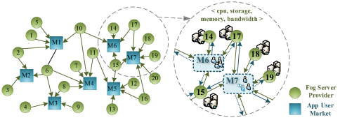
Figure 2: Resource management in fog computing.

Consider 20 fog service providers (FSPs) and 7 app user markets (AUMs), as shown in Figure 2. Each FSP can provide memory, bandwidth, CPU, or storage to AUMs. As a player, each fog server provider needs to determine how many resources to provide to app user markets in order to maximize its own benefits. That is, as a strategy in competition, FSP $i$ provides $a_{i}\in\mathbb{R}^{n_{i}}$ quantity of resources to the $n_{i}$ AUMs it connects. The connection relationship between the FSP and the AUM is denoted by a matrix $W$, which is a bipartite graph.

The extremely low-information environment is mainly caused by two reasons: cost and price. The local cost function of FSP $i$ is $\mathcal{C}_{i}\left(a_{i}\right)$ but the specific form is usually very complicated. The cost may come from many factors such as hardware, software, manpower, etc. Operations such as obtaining gradients in such a multi-coupled form will cause serious computational resource consumption. Moreover, what we only know and care about is the value of the cost, so directly operating on the cost value can reduce the occupation of computing resources. The price is determined by the relationship between supply and demand in the market. In real applications, FSP usually cannot know the specific form of the market pricing function, and in a market-based mechanism, resource supply and demand are dynamically changing, only the value of current price in the market is available to all players. Therefore, after FSP provides some kinds of resources to the market, the feedback which can be received from the market is their own profit value under this strategy. Overall, FSP compete with each other for market share to maximize their own profits, that is, in this networked fog resource management competition, each FSP aims to solve

$$\max_{a_{i}\in\mathcal{A}_{i}}(P(W\mathbf{a})-\mathcal{C}_{i}(a_{i}))W_{i}a_{i}$$

given the other providers’ profile $\mathbf{a}_{-i}$.

We simulate the two scenarios of known loss probability and unknown loss probability, respectively. Throughout this section, the empirical performance of OGD-lb in the expected sense is averaged over 10 paths.

6.2 Simulations with Known Loss Probability

We run Algorithm 1 with $\gamma_{i,k}={1}/{(k^{b}p_{i})}$ and $\delta_{k}=k^{-c}$. Firstly, we set $b=0.7$, $c=8/25$, $p_{i}=0.6$ and display the sublinear expectation-valued regret in Figure 3, which implies that algorithm OGD-lb meets the no-regret property. In other words, the online scheme is performing at least as well as any static strategy.

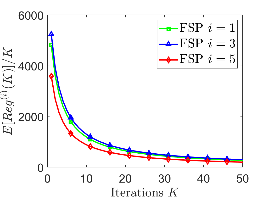
Figure 3: Average regret $\mathbb{E}\left[\mathcal{R}eg^{(i)}(K)\right]/K$ with update probability $p_{i}=0.6,i\in\{1,3,5\}$.

Next, keep $b=0.7$, $c=8/25$ and $p_{i}=0.6$ unchanged. Algorithm 1 is run by a single path and the result is demonstrated in Figure 4, which shows that the actions generated by OGD-lb will converge almost surely to the Nash equilibrium. But due to the lossy bandits, the curve will sometimes updated and sometimes unchanged.

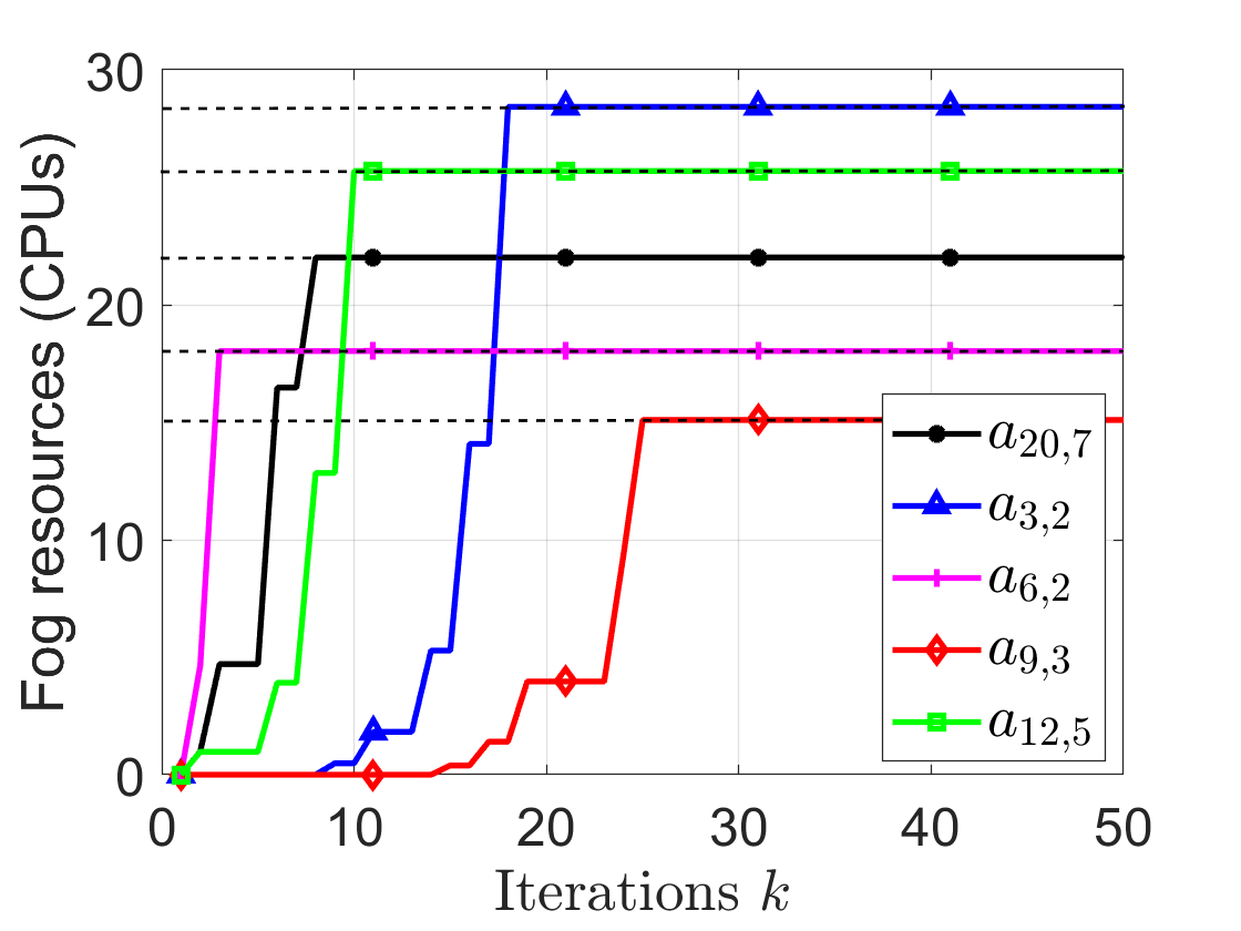
Figure 4: The trajectories of the decisions of some fog server providers, where $a_{i,j}$ represents the amount of CPUs supplied by FSP $i$ to AUM $j$, the Nash equilibrium is denoted by the dotted line.

We further keep $c=8/25$ to explore the influence of $p_{i}$ and $b$ on the convergence rate of the algorithm. As shown in Figure 5, the convergence rate increases as $p_{i}$ decreases. This is because increasing $p_{i}$ means that the bandit feedback from the AUM is more likely to be received by the FSP, that is, the algorithm update frequency is increased, and the convergence is accelerated. Moreover, we can see from Figure 6 that the convergence rate will increase as $b$ decreases. This is because decreasing $b$ will increase the update step-size.

Figure 5: The trajectories of $\sum_{i\in\mathcal{N}}\mathbb{E}\left[\|{\hat{a}_{i,k}}-{a^{*}}\|^{2}\right]$ with different update probabilities.

Figure 6: The trajectories of $\sum_{i\in\mathcal{N}}\mathbb{E}\left[\|{\hat{a}_{i,k}}-{a^{*}}\|^{2}\right]$ with different $b$.

Finally, let $\frac{\mathbb{E}\left[\|a_{k}-a^{*}\|\right]}{\|a^{*}\|}\leq\varepsilon$ and $p_{i}=P,i\in\mathcal{N}$. We investigate the iterations required for the player to reach the specified accuracy $\varepsilon$ under different probabilities, and the corresponding number of times the feedback information is received. It can be seen from Figure 7 that when $p_{i}$ is close to $0.8$, the number of iterations required to reach the accuracy $\varepsilon=0.01$ reaches the bottom. Therefore, if human intervention is allowed in applications, we can choose an appropriate update probability (such as $p_{i}=0.8$) instead of synchronous updates. This will greatly reduce the consumption of computing and communication resources.

Figure 7: Iterations vs Update times. (Where $p_{i}=P,i\in\mathcal{N}$ and ${\mathbb{E}\left[\|a_{k}-a^{*}\|\right]}/{\|a^{*}\|}\leq\varepsilon$. Iter denote the iterations required for the players to reach the accuracy of $\varepsilon$ under different probabilities. Upd denote the number of times that players update their actions.)

6.3 Simulations with Unknown Loss Probability

Consider Algorithm 1 with step-size $\gamma_{i,k}={1}/{(\Gamma_{i}^{k})^{q}}$, where $\Gamma_{i}^{k}=\sum_{t=1}^{k}I_{i}^{t}$, $q\in(1/2,1]$, and perturbation radius $\delta_{k}=k^{-c}$. Firstly, let $q=0.7$ and $c=8/25$. Performing Algorithm 1 with a single path, the result is shown in Figure 8, which shows that the actions generated by OGD-lb converge almost surely to the Nash equilibrium. But due to the lossy bandits, the curve will sometimes updated and sometimes unchanged.

Figure 8: The trajectories of the decisions of some fog server providers, where $a_{i,j}$ represents the amount of CPUs supplied by FSP $i$ to AUM $j$, the Nash equilibrium is denoted by the dotted line.

Next, we explore the regret and convergence rate of the algorithm in the unknown bandit feedback probability situation through simulations. We set $q=0.7$ and $c=8/25$, and display the expectation-valued regret versus the time horizon $K$ in Figure 9, which shows that the average regret converges sub-linearly, i.e., OGD-lb is a no-regret algorithm.

Figure 9: Average regret $\mathbb{E}\left[\mathcal{R}eg^{(i)}(K)\right]/K$ with update probability $p_{i}=0.8,i\in\{2,4,6\}$.

Then we set $c=8/25$ and investigate how do $q$ and $p_{i}$ influence the algorithm performance. It is seen from Figure 10 that the convergence rate increases as $q$ decreases. This is because decreasing $q$ increases the update step-size. We can see from Figure 11 that the convergence rate increases as $p_{i}$ decreases. This is because increasing $p_{i}$ increases the probability of FSP receiving feedback from the AUM, which increases the frequency of algorithm updates and accelerates convergence.

Figure 10: The trajectories of $\sum_{i\in\mathcal{N}}\mathbb{E}\left[\|{\hat{a}_{i,k}}-{a^{*}}\|^{2}\right]$ with different $q$.

Figure 11: The trajectories of $\sum_{i\in\mathcal{N}}\mathbb{E}\left[\|{\hat{a}_{i,k}}-{a^{*}}\|^{2}\right]$ with different update probabilities.

7 Conclusion

This paper considered bandit online learning for repeated stage games and proposed a novel no-regret algorithm called Online Gradient Descent with lossy bandits (OGD-lb). For concave games, we demonstrated that the algorithm meets the no-regret property with a proper selection of step-size. Furthermore, we showed that for strictly monotone games, the actions generated by OGD-lb can converge to a Nash equilibrium with probability 1 even when the bandit loss probability is unknown. Moreover, we derived an upper bound of the convergence rate for strongly monotone games, which can reach the same order of the algorithm without information loss. Finally, we applied the proposed method to the resource management game in fog computing.

References

• [1] Elad Hazan et al. Introduction to online convex optimization. Foundations and Trends® in Optimization, 2(3-4):157–325, 2016.
• [2] H Brendan McMahan, Gary Holt, David Sculley, Michael Young, Dietmar Ebner, Julian Grady, Lan Nie, Todd Phillips, Eugene Davydov, Daniel Golovin, et al. Ad click prediction: a view from the trenches. In Proceedings of the 19th ACM SIGKDD international conference on Knowledge discovery and data mining (KDD), pages 1222–1230, 2013.
• [3] Antoine Lesage-Landry, Iman Shames, and Joshua A. Taylor. Predictive online convex optimization. Automatica, 113:108771, 2020.
• [4] Tianyi Chen, Qing Ling, and Georgios B. Giannakis. An online convex optimization approach to proactive network resource allocation. IEEE Transactions on Signal Processing, 65(24):6350–6364, 2017.
• [5] Shai Shalev-Shwartz et al. Online learning and online convex optimization. Foundations and Trends® in Machine Learning, 4(2):107–194, 2012.
• [6] Xiao Xu and Qing Zhao. Distributed no-regret learning in multiagent systems: Challenges and recent developments. IEEE Signal Processing Magazine, 37(3):84–91, 2020.
• [7] Yan Zhang, Yi Zhou, Kaiyi Ji, and Michael M. Zavlanos. A new one-point residual-feedback oracle for black-box learning and control. Automatica, 136:110006, 2022.
• [8] Shai Shalev-shwartz and Yoram Singer. Convex repeated games and Fenchel duality. In Advances in Neural Information Processing Systems (NIPS), volume 19, 2006.
• [9] Deming Yuan, Yiguang Hong, Daniel W.C. Ho, and Guoping Jiang. Optimal distributed stochastic mirror descent for strongly convex optimization. Automatica, 90:196–203, 2018.
• [10] Sanjeev Arora, Elad Hazan, and Satyen Kale. The multiplicative weights update method: a meta-algorithm and applications. Theory of Computing, 8(1):121–164, 2012.
• [11] Adam Kalai and Santosh Vempala. Efficient algorithms for online decision problems. Journal of Computer and System Sciences, 71(3):291–307, 2005.
• [12] Martin Zinkevich. Online convex programming and generalized infinitesimal gradient ascent. In Proceedings of the 20th International Conference on Machine Learning (ICML), pages 928–936, 2003.
• [13] Elad Hazan, Amit Agarwal, and Satyen Kale. Logarithmic regret algorithms for online convex optimization. Machine Learning, 69(2-3):169–192, 2007.
• [14] Andrea Simonetto, Emiliano Dall’Anese, Julien Monteil, and Andrey Bernstein. Personalized optimization with user’s feedback. Automatica, 131:109767, 2021.
• [15] Farzad Salehisadaghiani, Wei Shi, and Lacra Pavel. Distributed Nash equilibrium seeking under partial-decision information via the alternating direction method of multipliers. Automatica, 103:27–35, 2019.
• [16] Zijie Zheng, Lingyang Song, Zhu Han, Geoffrey Ye Li, and H. Vincent Poor. Game theory for big data processing: Multi-leader multi-follower game-based ADMM. IEEE Transactions on Signal Processing, 66(15):3933–3945, 2018.
• [17] Peng Yi and Lacra Pavel. An operator splitting approach for distributed generalized Nash equilibria computation. Automatica, 102:111–121, 2019.
• [18] Barbara Franci and Sergio Grammatico. Stochastic generalized Nash equilibrium seeking in merely monotone games. IEEE Transactions on Automatic Control, pages 1–1, 2021.
• [19] Barbara Franci and Sergio Grammatico. Training generative adversarial networks via stochastic Nash games. IEEE Transactions on Neural Networks and Learning Systems, 2021.
• [20] Bolin Gao and Lacra Pavel. Continuous-time discounted mirror descent dynamics in monotone concave games. IEEE Transactions on Automatic Control, 66(11):5451–5458, 2021.
• [21] Jinlong Lei, Uday V. Shanbhag, and Jie Chen. Distributed computation of Nash equilibria for monotone aggregative games via iterative regularization. In 59th IEEE Conference on Decision and Control (CDC), pages 2285–2290, 2020.
• [22] Maojiao Ye, Guoqiang Hu, and Frank L Lewis. Nash equilibrium seeking for N-coalition non-cooperative games. Automatica, 95:266–272, 2018.
• [23] Xianlin Zeng, Jie Chen, Shu Liang, and Yiguang Hong. Generalized nash equilibrium seeking strategy for distributed nonsmooth multi-cluster game. Automatica, 103:20–26, 2019.
• [24] Nicolo Cesa-Bianchi and Gábor Lugosi. Prediction, learning, and games. Cambridge university press, 2006.
• [25] Geoffrey J Gordon, Amy Greenwald, and Casey Marks. No-regret learning in convex games. In Proceedings of the 25th International Conference on Machine Learning (ICML), pages 360–367, 2008.
• [26] Constantinos Daskalakis, Alan Deckelbaum, and Anthony Kim. Near-optimal no-regret algorithms for zero-sum games. In Proceedings of the 22th Annual ACM-SIAM Symposium on Discrete Algorithms (SODA), pages 235–254, 2011.
• [27] Michael Maskery, Vikram Krishnamurthy, and Qing Zhao. Decentralized dynamic spectrum access for cognitive radios: Cooperative design of a non-cooperative game. IEEE Transactions on Communications, 57(2):459–469, 2009.
• [28] Zhengyuan Zhou, Panayotis Mertikopoulos, Susan Athey, Nicholas Bambos, Peter W Glynn, and Yinyu Ye. Learning in games with lossy feedback. In Advances in Neural Information Processing Systems (NIPS), volume 31, 2018.
• [29] Yurii Nesterov and Vladimir Spokoiny. Random gradient-free minimization of convex functions. Foundations of Computational Mathematics, 17(2):527–566, 2017.
• [30] Xuanyu Cao and K. J. Ray Liu. Online convex optimization with time-varying constraints and bandit feedback. IEEE Transactions on Automatic Control, 64(7):2665–2680, 2019.
• [31] Xinlei Yi, Xiuxian Li, Tao Yang, Lihua Xie, Tianyou Chai, and Karl Henrik Johansson. Distributed bandit online convex optimization with time-varying coupled inequality constraints. IEEE Transactions on Automatic Control, 66(10):4620–4635, 2021.
• [32] Deming Yuan, Alexandre Proutiere, and Guodong Shi. Distributed online linear regressions. IEEE Transactions on Information Theory, 67(1):616–639, 2021.
• [33] Xuanyu Cao and Tamer Başar. Decentralized online convex optimization based on signs of relative states. Automatica, 129:109676, 2021.
• [34] Jingyi Zhu. Hessian-aided random perturbation (HARP) using noisy zeroth-order oracles. IEEE Transactions on Neural Networks and Learning Systems, 2021.
• [35] James C Spall. A one-measurement form of simultaneous perturbation stochastic approximation. Automatica, 33(1):109–112, 1997.
• [36] Jane Wei Huang, Hassan Mansour, and Vikram Krishnamurthy. A dynamical games approach to transmission-rate adaptation in multimedia wlan. IEEE Transactions on Signal Processing, 58(7):3635–3646, 2010.
• [37] Abraham D. Flaxman, Adam Tauman Kalai, and H. Brendan McMahan. Online convex optimization in the bandit setting: Gradient descent without a gradient. In Proceedings of the 16th Annual ACM-SIAM Symposium on Discrete Algorithms (SODA), page 385–394, 2005.
• [38] Jinlong Lei, Peng Yi, Yiguang Hong, Jie Chen, and Guodong Shi. Online convex optimization over Erdos-Renyi random networks. In Advances in Neural Information Processing Systems (NIPS), volume 33, pages 15591–15601, 2020.
• [39] Amélie Heliou, Johanne Cohen, and Panayotis Mertikopoulos. Learning with bandit feedback in potential games. In Advances in Neural Information Processing Systems (NIPS), volume 30, 2017.
• [40] Mario Bravo, David Leslie, and Panayotis Mertikopoulos. Bandit learning in concave N-person games. In Advances in Neural Information Processing Systems (NIPS), volume 31, 2018.
• [41] Amélie Héliou, Panayotis Mertikopoulos, and Zhengyuan Zhou. Gradient-free online learning in games with delayed rewards. In Proceedings of the 37th International Conference on Machine Learning (ICML-20), pages 1–11, 2020.
• [42] Yuanyuan Shi and Baosen Zhang. No-regret learning in Cournot games. arXiv preprint arXiv:1906.06612, 2019.
• [43] Wenbo Wang, Amir Leshem, Dusit Niyato, and Zhu Han. Decentralized learning for channel allocation in IoT networks over unlicensed bandwidth as a contextual multi-player multi-armed bandit game. IEEE Transactions on Wireless Communications, pages 1–1, 2021.
• [44] Yanli Xu. Gradient-free scheduling of fog computation for marine data feedback. IEEE Internet of Things Journal, 8(7):5657–5668, 2020.
• [45] Shihao Shen, Yiwen Han, Xiaofei Wang, and Yan Wang. Computation offloading with multiple agents in edge-computing–supported IoT. ACM Transactions on Sensor Networks (TOSN), 16(1):1–27, 2019.
• [46] Bingcong Li, Tianyi Chen, and Georgios B. Giannakis. Secure mobile edge computing in IoT via collaborative online learning. IEEE Transactions on Signal Processing, 67(23):5922–5935, 2019.
• [47] Tianyi Chen and Georgios B Giannakis. Bandit convex optimization for scalable and dynamic IoT management. IEEE Internet of Things Journal, 6(1):1276–1286, 2018.
• [48] Wenting Liu, Jinlong Lei, and Peng Yi. No-regret learning for repeated concave games with lossy bandits. In 2021 60th IEEE Conference on Decision and Control (CDC), pages 936–941. IEEE, 2021.
• [49] J Ben Rosen. Existence and uniqueness of equilibrium points for concave N-person games. Econometrica: Journal of the Econometric Society, pages 520–534, 1965.
• [50] Gesualdo Scutari, Daniel P Palomar, Francisco Facchinei, and Jong-Shi Pang. Convex optimization, game theory, and variational inequality theory. IEEE Signal Processing Magazine, 27(3):35–49, 2010.
• [51] Kai Lai Chung. On a stochastic approximation method. The Annals of Mathematical Statistics, pages 463–483, 1954.
• [52] Kunal Srivastava and Angelia Nedic. Distributed asynchronous constrained stochastic optimization. IEEE Journal of Selected Topics in Signal Processing, 5(4):772–790, 2011.