Distributed coordination for seeking the optimal Nash equilibrium of aggregative games

Abstract

This paper aims to design a distributed coordination algorithm for solving a multi-agent decision problem with a hierarchical structure. The primary goal is to search the Nash equilibrium of a noncooperative game such that each player has no incentive to deviate from the equilibrium under its private objective. Meanwhile, the agents can coordinate to optimize the social cost within the set of Nash equilibria of the underlying game. Such an optimal Nash equilibrium problem can be modeled as a distributed optimization problem with variational inequality constraints. We consider the scenario where the objective functions of both the underlying game and social cost optimization problem have a special aggregation structure. Since each player only has access to its local objectives while cannot know all players’ decisions, a distributed algorithm is highly desirable. By utilizing the Tikhonov regularization and dynamical averaging tracking technique, we propose a distributed coordination algorithm by introducing an incentive term in addition to the gradient-based Nash equilibrium seeking, so as to intervene players’ decisions to improve the system efficiency. We prove its convergence to the optimal Nash equilibrium of a monotone aggregative game with simulation studies.

I Introduction

Consider a group of players $\mathcal{N}=\{1,\cdots,N\}$, where each player $i\in\mathcal{N}$ decides its strategy $x_{i}\in\mathbb{R}^{m}$. The $i$th player is characterized by two cost functions $f_{i}(x_{i},\bar{x}):\mathbb{R}^{2m}\rightarrow\mathbb{R}$ and $g_{i}(x_{i},\bar{x}):\mathbb{R}^{2m}\rightarrow\mathbb{R}$, which depend on $x_{i}$ and the aggregate $\bar{x}=\frac{1}{N}\sum_{i=1}^{N}x_{i}$. The primary goal of the players is to seek a Nash equilibrium (NE) in an aggregative game $P_{a}$, i.e., player $i$ solves the following optimization problem given other players’ decisions,

$$\min_{x_{i}\in\mathbb{R}^{m}}f_{i}\Big{(}x_{i},\tfrac{1}{N}x_{i}+\tfrac{1}{N}\sum_{j\neq i}x_{j}\Big{)}. P_{a}$$ ()

A profile $\mathbf{\tilde{x}}=[\tilde{x}_{1}^{T},\cdots,\tilde{x}_{N}^{T}]^{T}$ is a Nash equilibrium when

$$\tilde{x}_{i}\in\arg\min_{x_{i}\in\mathbb{R}^{m}}f_{i}\Big{(}x_{i},\tfrac{1}{N}x_{i}+\tfrac{1}{N}\sum_{j\neq i}\tilde{x}_{j}\Big{)},~{}\forall i\in\mathcal{N}$$

Denote by $X^{*}\subseteq\mathbb{R}^{mN}$ the set of Nash equilibria to ($P_{a}$). The secondary goal is to cooperatively solve the distributed constrained aggregative optimization problem:

$$\min_{\mathbf{x}=[{x}_{1}^{T},\cdots,{x}_{N}^{T}]^{T}}g(\mathbf{x})=\sum_{i=1}^{N}g_{i}(x_{i},\bar{x}),s.t.~{}\mathbf{x}\in X^{*}. P_{b}$$ ()

The ultimate goal of this work is to design a distributed coordination algorithm to seek a $\mathbf{x}^{*}\in\arg\min_{\mathbf{x}\in X^{*}}\{g(\mathbf{x})\}$ of ($P_{b}$).

We consider the aforementioned problem since game theory is increasingly applied to control and decision problems over networks such as network load balancing [1], smart grids [2], and intelligent transportation systems[3]. Meanwhile, the class of aggregative games in ($P_{a}$) has attracted significant attention recently due to its wide applications, such as charging management plug-in electric vehicles[4, 5], demand-response [6, 7], spectrum sharing game [8] and public goods problem [9]. Hence, seeking NE of aggregative games is also of interest, and we list [10, 11, 12, 13] for a few.

Even though NE represents the incentive compatibility state of a game, it can be non-unique for a variety of problems. For example, there exist two equilibria in the stag hunt game, and [14] proves that in a congestion game, the number of Nash equilibria is exponential in the number of users and routes. The efficiency of Nash equilibria has drawn much attention for decades, since Nash equilibria do not always optimize the overall system performance or lead to the lowest social cost (like ($P_{b}$)), taking the Prisoner’s Dilemma as a famous example. To measure the efficiency of different Nash equilibria, [14] proposes to use the ratio between the social cost of the worst Nash equilibrium and the global optimum, called “Price of Anarchy” (PoA). Within this avenue, [15] studies a noncooperative spectrum sharing game with two players and provides the upper bound of PoA at a high signal to noise ratio. [16] considers aggregative charging games in smart grids, and provides the upper bounds of PoA for three types of charging price functions. In addition to considering the efficiency under the worst Nash equilibrium, how to obtain a best Nash equilibrium that optimizes the social welfware/cost is also very meaningful, and is referred as the optimal NE problem [17].

However, we cannot expect that the existing NE seeking algorithms (like in [10], [12], and [13]) can naturally converge to the optimal NE. As such, certain intervention and control must be imposed. There are a few works studying how to intervening in the players to obtain an optimal NE. For example, [18] proposes a completely uncoupled learning rule to select an efficient NE in a Pareto optimal sense. Based on [18], [19] further proposes and proves learning procedures that can lead to a Pareto optimal action profile for repeated games, but the converged profile is not necessarily an NE. The authors of [20] propose to affect players’ strategies by imposing an external incentive target. This method is able to converge to an optimal NE, which however necessitates a central planner and needs to change the players’ objectives. Recently, [17] studies an optimization problem with variational inequality constraints, and demonstrates that the optimal NE problem can be reformulated as it. Based on the Tikhonov trajectory, it also develops a converging algorithm, but needs either a center or requires full information of all players.

Motivated by the appealing properties of distributed algorithms for large-scale networks, we propose solving the problem ($P_{b}$) over a network. With the distributed algorithm, each player preserves its local objective functions $f_{i}$ and $g_{i}$, and needs no center to collect and broadcast the aggregation variable. By applying the gradient tracking technique, we propose a distributed and single-timescale algorithm for this problem with provable convergence guarantee.

The rest of the paper is organized as follows. We list the standing assumptions of problems ($P_{a}$) and ($P_{b}$) in Section II, and then design a distributed algorithm along with the main results in Section III. We validate the proposed algorithm through numerical simulations in Section IV, and conclude the paper in Section V.

Notations. Let $\mathbf{x}=[x_{1}^{T},\cdots,x_{N}^{T}]^{T}$ stack the vectors $x_{1},\cdots,x_{N}$, and $x_{-i}=[x_{1}^{T},\cdots,x_{i-1}^{T},x_{i+1}^{T},\cdots,x_{N}^{T}]^{T}$. Denote $\nabla_{1}f_{i}(x_{i},\bar{x})$ by $\nabla_{x_{i}}f_{i}(\cdot,\bar{x})$ and $\nabla_{2}f_{i}(x_{i},\bar{x})$ by $\nabla_{\bar{x}}f_{i}(x_{i},\cdot)$. Let $\|x\|$ denote the Euclidean two-norm. An $N$ dimension vector with all entries being one is denoted by $\mathbf{1}_{N}$, and the $m\times m$ identity matrix is denoted by $I_{m}$. Denote a graph by $\mathcal{G}=(\mathcal{N,E})$, where $\mathcal{N}$ is the set of nodes, and $\mathcal{E}\subseteq\mathcal{N}\times\mathcal{N}$ denotes the set of ordered pairs, called edges. A graph $\mathcal{G}$ is called undirected when for any edge $(i,j)\in\mathcal{E}$, there exists an edge $(j,i)\in\mathcal{E}$. An undirected graph $\mathcal{G}$ is called connected if there exists a path between any two nodes. Define the weighted adjacency matrix $W=[w_{ij}]_{i,j=1}^{N}$ of $\mathcal{G}$ as $w_{ij}>0$ if $(i,j)\in\mathcal{E}$ else $w_{ij}=0$.

II Standing Assumptions

We make the following assumptions on the problem ($P_{a}$).

Assumption 1.

For each player $i\in\mathcal{N},$

• $f_{i}\left(x_{i},\frac{1}{N}x_{i}+\frac{1}{N}\sum_{j\neq i}x_{j}\right)$ is convex in $x_{i}\in\mathbb{R}^{m}$ for every fixed $x_{-i}$;

• $f_{i}(\cdot,\beta)$ is continuously differentiable in $x_{i}\in\mathbb{R}^{m}$ for every fixed $\beta\in\mathbb{R}^{m}$, and $f_{i}(x_{i},\beta)$ is continuously differentiable in $\beta\in\mathbb{R}^{m}$ for every fixed $x_{i}\in\mathbb{R}^{m}$.

Let

$$\begin{split}\nabla_{1}f_{i}(x_{i},\bar{x})&=\nabla_{1}f_{i}(x_{i},\bar{x})+\frac{1}{N}\nabla_{2}f_{i}(x_{i},\bar{x}),~{}i\in\mathcal{N},\\ \nabla_{1}f(\mathbf{x,y})&=[\nabla_{1}f_{1}(x_{1},y_{1})^{T},\cdots,\nabla_{1}f_{N}(x_{N},y_{N})^{T}]^{T},\\ \nabla_{2}f(\mathbf{x,y})&=[\nabla_{2}f_{1}(x_{1},y_{1})^{T},\cdots,\nabla_{2}f_{N}(x_{N},y_{N})^{T}]^{T},\\ F(\mathbf{x})&=[\nabla f_{1}(x_{1},\bar{x})^{T},\cdots,\nabla f_{N}(x_{N},\bar{x})^{T}]^{T}\\ &=\nabla_{1}f(\mathbf{x},\mathbf{1}_{N}\otimes\bar{x})+\frac{1}{N}\nabla_{2}f(\mathbf{x},\mathbf{1}_{N}\otimes\bar{x}).\end{split}$$ (1)

Assumption 1 is a sufficient condition that guarantees the existence of an NE for ($P_{a}$). From [21], $\tilde{\mathbf{x}}$ is an NE if and only if it is a solution to the variational inequality $VI(\mathbb{R}^{mN},F)$,

$$F(\tilde{\mathbf{x}})^{T}(\mathbf{x}-\tilde{\mathbf{x}})\geq 0\text{~{}for all~{}}\mathbf{x}\in\mathbb{R}^{mN}.$$ (2)

The solution set of (2) is denoted as $SOL(\mathbb{R}^{mN},F)$.

Proposition 1.

Under Assumption 1, a vector $\tilde{\mathbf{{x}}}$ solves $VI(\mathbb{R}^{mN},F)$ if and only if $F(\tilde{\mathbf{x}})=0$.

We require the set of Nash equilibria to be nonempty, and impose some Lipschitz continuity conditions on the mappings defined in (1).

Assumption 2.

• The map $F(\mathbf{x})$ is $L_{F}$-Lipschitz continuous and monotone in $\mathbf{x}\in\mathbb{R}^{mN}$, and $\nabla_{1}f(\mathbf{x},\mathbf{y})+\frac{1}{N}\nabla_{2}f(\mathbf{x},\mathbf{y})$ is also $L_{F}$-Lipschitz continuous in $(\mathbf{x,y})\in\mathbb{R}^{mN}\times\mathbb{R}^{mN}$, i.e., for any $(\mathbf{x,y}),(\mathbf{x}^{\prime}\mathbf{y}^{\prime})\in\mathbb{R}^{mN}\times\mathbb{R}^{mN}$,

  $$\begin{split}&\|F(\mathbf{x})-F(\mathbf{x}^{\prime})\|\leq L_{F}\|\mathbf{x}-\mathbf{x}^{\prime}\|,\\ &(F(\mathbf{x})-F(\mathbf{x}^{\prime}))^{T}(\mathbf{x}-\mathbf{x}^{\prime})\geq 0,\\ &\Big{\|}\nabla_{1}f(\mathbf{x},\mathbf{y})+\frac{1}{N}\nabla_{2}f(\mathbf{x},\mathbf{y})-\nabla_{1}f(\mathbf{x}^{\prime},\mathbf{y}^{\prime})-\frac{1}{N}\nabla_{2}f(\mathbf{x}^{\prime},\mathbf{y}^{\prime})\Big{\|}\\ &\leq L_{F}(\|\mathbf{x}-\mathbf{x}^{\prime}\|+\|\mathbf{y}-\mathbf{y}^{\prime}\|).\end{split}$$

• $X^{*}$ is a nonempty set.

For problem ($P_{b}$), let

$$\nabla_{1}g_{i}(\mathbf{x}) =\nabla_{1}g_{i}(x_{i},\bar{x})+\frac{1}{N}\sum_{j=1}^{N}\nabla_{2}g_{j}(x_{j},\bar{x}),~{}i\in\mathcal{N},$$

$$\nabla_{1}g(\mathbf{x,y}) =[\nabla_{1}g_{1}(x_{1},y_{1})^{T},\cdots,\nabla_{1}g_{N}(x_{N},y_{N})^{T}]^{T},$$

$$\nabla_{2}g(\mathbf{x,y}) =[\nabla_{2}g_{1}(x_{1},y_{1})^{T},\cdots,\nabla_{2}g_{N}(x_{N},y_{N})^{T}]^{T},$$

$$\nabla g(\mathbf{x}) =\nabla_{1}g(\mathbf{x},\mathbf{1}_{N}\otimes\bar{x})+\frac{\mathbf{1}_{N}\mathbf{1}_{N}^{T}}{N}\otimes I_{m}\nabla_{2}g(\mathbf{x},\mathbf{1}_{N}\otimes\bar{x}).$$

We impose the following assumptions on $g(\mathbf{x})$.

Assumption 3.

• The global objective function $g$ is differentiable and $\mu_{g}$-strongly convex in $\mathbf{x}\in\mathbb{R}^{mN}$. Also, $\nabla g$ and $\nabla_{1}g(\mathbf{x},\mathbf{y})+\frac{\mathbf{1}_{N}\mathbf{1}_{N}^{T}}{N}\otimes I_{m}\nabla_{2}g(\mathbf{x},\mathbf{y})$ are $L_{1}$ Lipschitz continuous in $(\mathbf{x,y})\in\mathbb{R}^{mN}\times\mathbb{R}^{mN}$, i.e., for any $(\mathbf{x,y}),(\mathbf{x}^{\prime}\mathbf{y}^{\prime})\in\mathbb{R}^{mN}\times\mathbb{R}^{mN}$,

  $$\begin{split}&\|\nabla g(\mathbf{x})-\nabla g(\mathbf{x}^{\prime})\|\leq L_{1}\|\mathbf{x}-\mathbf{x}^{\prime}\|,\\ &(\nabla g(\mathbf{x})-\nabla g(\mathbf{x}^{\prime}))^{T}(\mathbf{x}-\mathbf{x}^{\prime})\geq\mu_{g}\|\mathbf{x}-\mathbf{x}^{\prime}\|^{2},\\ &\Bigg{\|}\nabla_{1}g(\mathbf{x},\mathbf{y})+\frac{\mathbf{1}_{N}\mathbf{1}_{N}^{T}}{N}\otimes I_{m}\nabla_{2}g(\mathbf{x},\mathbf{y})\\ &\quad-\nabla_{1}g(\mathbf{x}^{\prime},\mathbf{y}^{\prime})-\frac{\mathbf{1}_{N}\mathbf{1}_{N}^{T}}{N}\otimes I_{m}\nabla_{2}g(\mathbf{x}^{\prime},\mathbf{y}^{\prime})\Bigg{\|}\\ &\quad\leq L_{1}(\|\mathbf{x}-\mathbf{x}^{\prime}\|+\|\mathbf{y}-\mathbf{y}^{\prime}\|).\end{split}$$

• $\nabla_{2}g(\mathbf{x,y})$ is $L_{2}$ Lipschitz continuous in $(\mathbf{x,y})\in\mathbb{R}^{mN}\times\mathbb{R}^{mN}$, i.e., for any $(\mathbf{x,y}),(\mathbf{x}^{\prime}\mathbf{y}^{\prime})\in\mathbb{R}^{mN}\times\mathbb{R}^{mN}$,

  $$\left\|\nabla_{2}g(\mathbf{x},\mathbf{y})-\nabla_{2}g(\mathbf{x}^{\prime},\mathbf{y}^{\prime})\right\|\leq L_{2}(\|\mathbf{x}-\mathbf{x}^{\prime}\|+\|\mathbf{y}-\mathbf{y}^{\prime}\|).$$

Note that we only require the global function $g(\mathbf{x})$ to be strongly convex, while each local function $g_{i}(x_{i},\bar{x})$ is not necessarily strongly convex or convex. Since the objective function $g$ is strongly convex, ($P_{b}$) has a unique optimal solution, denoted as $\mathbf{x}^{*}$.

Let the interaction among the players be described by an undirected graph $\mathcal{G}=(\mathcal{N},\mathcal{E})$ with the adjacency matrix denoted by $W$. We impose the following conditions on $\mathcal{G}$.

Assumption 4.

The communication graph $\mathcal{G}$ is undirected and connected. Besides, the adjacency matrix $W=[w_{ij}]_{i,j=1}^{N}$ is nonnegative and doubly stochastic, i.e., $W\mathbf{1}_{N}=\mathbf{1}_{N}$ and $\mathbf{1}_{N}^{T}W=\mathbf{1}_{N}^{T}$.

III Distributed Algorithm and Main results

We propose a distributed Tikhonov regularized algorithm to compute the optimal NE as follows.

Algorithm 1 Distributed seeking for the optimal NE

Initialization: For each $i\in\mathcal{N}$, let $x_{i}^{0}\in\mathbb{R}^{m}$ and set $v_{i}^{0}=x_{i}^{0},y_{i}^{0}=\nabla_{2}g_{i}(x_{i}^{0},v_{i}^{0})$;
Iteration: for all $k\geq 0$,

$$x_{i}^{k+1} =x_{i}^{k}-\gamma_{k}\left(\nabla_{1}f_{i}(x_{i}^{k},v_{i}^{k})+\tfrac{1}{N}\nabla_{2}f_{i}(x_{i}^{k},v_{i}^{k})+\eta_{k}(\nabla_{1}g_{i}(x_{i}^{k},v_{i}^{k})+y_{i}^{k})\right),$$

$$v_{i}^{k+1} =\sum_{i=1}^{N}w_{ij}v_{i}^{k}+x_{i}^{k+1}-x_{i}^{k},$$

$$y_{i}^{k+1} =\sum_{i=1}^{N}w_{ij}y_{i}^{k}+\nabla_{2}g_{i}(x_{i}^{k+1},v_{i}^{k+1})-\nabla_{2}g_{i}(x_{i}^{k},v_{i}^{k}),$$

where $\gamma_{k},\eta_{k}$ are positive step-sizes.

In the algorithm, the local variables $v_{i}$ and $y_{i}$ are used to track the dynamical aggregate $\bar{x}$ and $\tfrac{1}{N}\sum_{i=1}^{N}\nabla_{2}g_{i}(x_{i},\bar{x})$, respectively. Then each player $i$ uses $\nabla_{1}f_{i}(x_{i}^{k},v_{i}^{k})+\frac{1}{N}\nabla_{2}f_{i}(x_{i}^{k},v_{i}^{k})$ as an estimate of the gradient $\nabla_{1}f_{i}(x_{i}^{k},\bar{x}^{k})$ to seek the NE of ($P_{a}$), and adds an incentive term $\nabla_{1}g_{i}(x_{i}^{k},v_{i}^{k})+y_{i}^{k}$ as an estimate of the gradient $\nabla_{1}g_{i}(\mathbf{x}^{k})$ to optimize the social cost.

Algorithm 1 can be represented compactly as follows:

$$\mathbf{x}^{k+1} =\mathbf{x}^{k}-\gamma_{k}\Big{(}\nabla_{1}f(\mathbf{x}^{k},\mathbf{v}^{k})+\frac{1}{N}\nabla_{2}f(\mathbf{x}^{k},\mathbf{v}^{k})$$

$$\quad\quad\quad\quad\quad+\eta_{k}(\nabla_{1}g(\mathbf{x}^{k},\mathbf{v}^{k})+\mathbf{y}^{k})\Big{)},$$ (3)

$$\mathbf{v}^{k+1} =W\otimes I_{m}\mathbf{v}^{k}+\mathbf{x}^{k+1}-\mathbf{x}^{k},$$ (4)

$$\mathbf{y}^{k+1} =W\otimes I_{m}\mathbf{y}^{k}+\nabla_{2}g(\mathbf{x}^{k+1},\mathbf{v}^{k+1})-\nabla_{2}g(\mathbf{x}^{k},\mathbf{v}^{k}).$$ (5)

We impose the following conditions on the step-sizes $\{\gamma_{k}\}$ and $\{\eta_{k}\}$.

Assumption 5.

(Step-size update rules) Set $\gamma_{k}=\frac{\gamma_{0}}{(k+1)^{a}}>0$ and $\eta_{k}=\frac{\eta_{0}}{(k+1)^{b}}>0$ for $k\geq 0$, where $a,b$ satisfy $0<b<a<1$ and $a+b<1$.

With the initial state $v_{i}^{0}=x_{i}^{0},y_{i}^{0}=\nabla_{2}g_{i}(x_{i}^{0},v_{i}^{0})$, similarly to [10, Lemma 2], we can easily obtain the following lemma.

Lemma 1.

Define $\bar{v}^{k}\triangleq{1\over N}\sum_{i=1}^{N}v_{i}^{k}$ and $\bar{y}^{k}\triangleq{1\over N}\sum_{i=1}^{N}y_{i}^{k}$. Under Assumption 4, we have that

$$\bar{v}^{k}=\bar{x}^{k},~{}\bar{y}^{k}=\frac{\mathbf{1}_{N}^{T}}{N}\otimes I_{m}\nabla_{2}g(\mathbf{x}^{k},\mathbf{v}^{k}),\quad\forall k\geq 0.$$

From Assumptions 2 and 3, we can easily obtain some properties of the regularized map $F+\eta_{k}\nabla g$.

Lemma 2.

Let Assumptions 2 and 3 hold. Then $F+\eta_{k}\nabla g$ is $(\eta_{k}\mu_{g})$-strongly monotone and $(L_{F}+\eta_{k}L_{1})$ Lipschitz continuous, and $\nabla_{1}f(\mathbf{x},\mathbf{y})+\tfrac{1}{N}\nabla_{2}f(\mathbf{x},\mathbf{y})+\eta_{k}\left(\nabla_{1}g(\mathbf{x},\mathbf{y})+\tfrac{\mathbf{1}_{N}\mathbf{1}_{N}^{T}}{N}\otimes I_{m}\nabla_{2}g(\mathbf{x},\mathbf{y})\right)$ is also $(L_{F}+\eta_{k}L_{1})$-Lipschitz continuous.

Since $F+\eta_{k}\nabla g$ is strongly monotone and Lipschitz continuous, there exists an unique solution $\mathbf{x}_{\eta_{k}}^{*}$ to $VI(\mathbb{R}^{mN},F+\eta_{k}\nabla g)$. The sequence $\{\mathbf{x}_{\eta_{k}}^{*}\}$ is called the Tikhonov trajectory of the Problem ($P_{b}$). In the following, we show that the trajectory asymptotically converges to the optimal solution to Problem ($P_{b}$), and provide the upper bound on the error $\|\mathbf{x}_{\eta_{k}}^{*}-\mathbf{x}_{\eta_{k-1}}^{*}\|$. The proof is similar to that of [17, Lemma 4.5], so we give the proof in Appendix for completeness. The established properties of the Tikhonov trajectory will be used in the convergence analysis of Algorithm 1.

Lemma 3.

(Properties of Tikhonov trajectory) Let Assumptions 1, 2, 3 and 5 hold. Then we have
(a) the sequence $\{\mathbf{x}_{\eta_{k}}^{*}\}$ converges to $\mathbf{x}^{*}$;
(b) there exists a scalar $C>0$ such that $\|\mathbf{x}_{\eta_{k}}^{*}-\mathbf{x}_{\eta_{k-1}}^{*}\|\leq\frac{C}{\mu_{g}}\Gamma_{k-1}$ for all $k\geq 1$, where $\Gamma_{k-1}=|1-\frac{\eta_{k-1}}{\eta_{k}}|$.

We use $\|\mathbf{x}^{k}-\mathbf{x}_{\eta_{k-1}}^{*}\|,\|\mathbf{v}^{k}-\mathbf{1}_{N}\otimes\bar{v}^{k}\|,\|\mathbf{y}^{k}-\mathbf{1}_{N}\otimes\bar{y}^{k}\|$ to show our convergence, of which the first term represents the distance between the iterate and the Tikhonov trajectory, the second term measures the consensus violation for the aggregate and the third term measures the consensus violation for the gradient of the global cost function. Define $\Delta_{k}=\left[\|\mathbf{x}^{k}-\mathbf{x}_{\eta_{k-1}}^{*}\|,\|\mathbf{v}^{k}-\mathbf{1}_{N}\otimes\bar{v}^{k}\|,\|\mathbf{y}^{k}-\mathbf{1}_{N}\otimes\bar{y}^{k}\|\right]^{T}$. The following result provides a recursive relation of the three metrics.

Proposition 2.

Consider Algorithm 1 under Assumptions 1-5. If $0<\gamma_{0}<1/(L_{F}+\eta_{0}L_{1})$, we have $\Delta_{k+1}\leq H_{k}\Delta_{k}+h_{k}$ for all $k\geq 1$, where $H_{k}=[H_{k,ij}]_{3\times 3},h_{k}=[h_{k,i}]_{3\times 1}$ are given by

$$H_{k,11}=1-\gamma_{k}\eta_{k}\mu_{g},~{}H_{k,12}=\gamma_{k}(L_{F}+\eta_{k}L_{1}),$$

$$H_{k,13}=H_{k,23}=\gamma_{k}\eta_{k},~{}H_{k,21}=2\gamma_{k}(L_{F}+\eta_{k}L_{1}),$$

$$H_{k,22}=\rho+\gamma_{k}(L_{F}+\eta_{k}L_{1}),~{}H_{k,31}=4L_{2}\gamma_{k}(L_{F}+\eta_{k}L_{1}),$$

$$H_{k,32}=L_{2}\|W-I_{N}\|+2L_{2}\gamma_{k}(L_{F}+\eta_{k}L_{1}),$$

$$H_{k,33}=\rho+2L_{2}\gamma_{k}\eta_{k},$$

$$h_{k,1}=\tfrac{C}{\mu_{g}}\Gamma_{k-1},~{}h_{k,2}=\tfrac{2\gamma_{k}C(L_{F}+\eta_{k}L_{1})}{\mu_{g}}\Gamma_{k-1},$$

$$h_{k,3}=\tfrac{4L_{2}\gamma_{k}C(L_{F}+\eta_{k}L_{1})}{\mu_{g}}\Gamma_{k-1}.$$

Proof. First we show $\Delta_{k+1,1}\leq\sum_{i=1}^{3}H_{k,1i}\Delta_{k,i}+h_{k,1}$. From the definition of $\mathbf{x}_{\eta_{k}}^{*}$ and Proposition 1, we know that $F(\mathbf{x}_{\eta_{k}}^{*})+\eta_{k}\nabla g(\mathbf{x}_{\eta_{k}}^{*})=0$. By (3),

$$\|\mathbf{x}^{k+1}-\mathbf{x}_{\eta_{k}}^{*}\|=\big{\|}\mathbf{x}^{k}-\gamma_{k}\big{(}\nabla_{1}f(\mathbf{x}^{k},\mathbf{v}^{k})+\tfrac{1}{N}\nabla_{2}f(\mathbf{x}^{k},\mathbf{v}^{k})$$

$$+\eta_{k}(\nabla_{1}g(\mathbf{x}^{k},\mathbf{v}^{k})+\mathbf{y}^{k})\big{)}-\mathbf{x}_{\eta_{k}}^{*}+\gamma_{k}\left(F(\mathbf{x}_{\eta_{k}}^{*})+\eta_{k}\nabla g(\mathbf{x}_{\eta_{k}}^{*})\right)\big{\|}$$

$$\leq\Big{\|}\mathbf{x}^{k}-\gamma_{k}\left(F(\mathbf{x}^{k})+\eta_{k}\nabla g(\mathbf{x}^{k})\right)-\mathbf{x}_{\eta_{k}}^{*}$$

$$+\gamma_{k}\left(F(\mathbf{x}_{\eta_{k}}^{*})+\eta_{k}\nabla g(\mathbf{x}_{\eta_{k}}^{*})\right)\Big{\|}+\gamma_{k}\Big{\|}F(\mathbf{x}^{k})+\eta_{k}\nabla g(\mathbf{x}^{k})$$ (6)

$$-\Big{(}\nabla_{1}f(\mathbf{x}^{k},\mathbf{v}^{k})+\frac{1}{N}\nabla_{2}f(\mathbf{x}^{k},\mathbf{v}^{k})$$

$$+\eta_{k}(\nabla_{1}g(\mathbf{x}^{k},\mathbf{v}^{k})+\mathbf{1}_{N}\otimes\bar{y}^{k})\Big{)}\Big{\|}+\gamma_{k}\eta_{k}\left\|\mathbf{1}_{N}\otimes\bar{y}^{k}-\mathbf{y}^{k}\right\|.$$

Since $0<\gamma_{0}<1/(L_{F}+\eta_{0}L_{1})$ and $\{\eta_{k}\},\{\gamma_{k}\}$ are non-increasing sequence, we have that

$$0<\gamma_{k}<\gamma_{0}<1/(L_{F}+\eta_{0}L_{1})<1/(L_{F}+\eta_{k}L_{1}),\quad\forall k\geq 0.$$

Then by recalling that $F+\eta_{k}\nabla g$ is $(\eta_{k}\mu_{g})$-strongly monotone and $(L_{F}+\eta_{k}L_{1})$ Lipschitz continuous from Lemma 2, and using [22, Lemma 3], we have

$$\begin{split}&\Big{\|}\mathbf{x}^{k}-\gamma_{k}\left(F(\mathbf{x}^{k})+\eta_{k}\nabla g(\mathbf{x}^{k})\right)-\mathbf{x}_{\eta_{k}}^{*}\\ &+\gamma_{k}\left(F(\mathbf{x}_{\eta_{k}}^{*})+\eta_{k}\nabla g(\mathbf{x}_{\eta_{k}}^{*})\right)\Big{\|}\leq(1-\gamma_{k}\eta_{k}\mu_{g})\|\mathbf{x}^{k}-\mathbf{x}_{\eta_{k}}^{*}\|.\end{split}$$ (7)

By Lemma 1, we have

$$\begin{split}&\nabla_{1}f(\mathbf{x}^{k},\mathbf{v}^{k})+\frac{1}{N}\nabla_{2}f(\mathbf{x}^{k},\mathbf{v}^{k})+\eta_{k}(\nabla_{1}g(\mathbf{x}^{k},\mathbf{v}^{k})+\mathbf{1}_{N}\otimes\bar{y}^{k})\\ &=\nabla_{1}f(\mathbf{x}^{k},\mathbf{v}^{k})+\frac{1}{N}\nabla_{2}f(\mathbf{x}^{k},\mathbf{v}^{k})\\ &+\eta_{k}\left(\nabla_{1}g(\mathbf{x}^{k},\mathbf{v}^{k})+\frac{\mathbf{1}_{N}\mathbf{1}_{N}^{T}}{N}\otimes I_{m}\nabla_{2}g(\mathbf{x}^{k},\mathbf{v}^{k})\right).\end{split}$$

Using the definition of $F(\mathbf{x}^{k})$ and $\nabla g(\mathbf{x}^{k})$ and $\bar{v}^{k}=\bar{x}^{k}$ in Lemma 1, we can further obtain that

$$\begin{split}&F(\mathbf{x}^{k})+\eta_{k}\nabla g(\mathbf{x}^{k})=\nabla_{1}f(\mathbf{x}^{k},\mathbf{1}_{N}\otimes\bar{v}^{k})+\frac{1}{N}\nabla_{2}f(\mathbf{x}^{k},\mathbf{1}_{N}\otimes\bar{v}^{k})\\ &+\eta_{k}\left(\nabla_{1}g(\mathbf{x}^{k},\mathbf{1}_{N}\otimes\bar{v}^{k})+\frac{\mathbf{1}_{N}\mathbf{1}_{N}^{T}}{N}\otimes I_{m}\nabla_{2}g(\mathbf{x}^{k},\mathbf{1}_{N}\otimes\bar{v}^{k})\right).\end{split}$$

Then by recalling the Lipschitz continuity of $\nabla_{1}f(\mathbf{x},\mathbf{y})+\frac{1}{N}\nabla_{2}f(\mathbf{x},\mathbf{y})+\eta_{k}\left(\nabla_{1}g(\mathbf{x},\mathbf{y})+\frac{\mathbf{1}_{N}\mathbf{1}_{N}^{T}}{N}\otimes I_{m}\nabla_{2}g(\mathbf{x},\mathbf{y})\right)$ from Lemma 2, we have

$$\begin{split}&\gamma_{k}\Big{\|}F(\mathbf{x}^{k})+\eta_{k}\nabla g(\mathbf{x}^{k})-\Big{[}\nabla_{1}f(\mathbf{x}^{k},\mathbf{v}^{k})\\ &+\frac{1}{N}\nabla_{2}f(\mathbf{x}^{k},\mathbf{v}^{k})+\eta_{k}(\nabla_{1}g(\mathbf{x}^{k},\mathbf{v}^{k})+\mathbf{1}_{N}\otimes\bar{y}^{k})\Big{]}\Big{\|}\\ &\leq\gamma_{k}(L_{F}+\eta_{k}L_{1})\|\mathbf{v}^{k}-\mathbf{1}_{N}\otimes\bar{v}^{k}\|.\end{split}$$ (8)

This combined with (III) and (7) produces

$$\begin{split}&\|\mathbf{x}^{k+1}-\mathbf{x}_{\eta_{k}}^{*}\|\leq(1-\gamma_{k}\eta_{k}\mu_{g})\|\mathbf{x}^{k}-\mathbf{x}_{\eta_{k}}^{*}\|\\ &+\gamma_{k}(L_{F}+\eta_{k}L_{1})\|\mathbf{v}^{k}-\mathbf{1}_{N}\otimes\bar{v}^{k}\|+\gamma_{k}\eta_{k}\|\mathbf{1}_{N}\otimes\bar{y}^{k}-\mathbf{y}^{k}\|.\end{split}$$ (9)

Adding and substracting $\mathbf{x}_{\eta_{k-1}}^{*}$ in the first term, noting that $1-\gamma_{k}\eta_{k}\mu_{g}<1$, and using Lemma 3, we obtain the desired inequality.

Next, we show that $\Delta_{k+1,2}\leq\sum_{i=1}^{3}H_{k,2i}\Delta_{k,i}+h_{k,2}$. Since $W$ is doubly stochastic, by using (4) and $\big{\|}I_{mN}-\tfrac{\mathbf{1}_{N}\mathbf{1}_{N}^{T}}{N}\otimes I_{m}\big{\|}=1$, we have

$$\begin{split}&\|\mathbf{v}^{k+1}-\mathbf{1}_{N}\otimes\bar{v}^{k+1}\|=\Big{\|}W\otimes I_{m}\mathbf{v}^{k}+\mathbf{x}^{k+1}-\mathbf{x}^{k}\\ &-\tfrac{\mathbf{1}_{N}\mathbf{1}_{N}^{T}}{N}\otimes I_{m}(W\otimes I_{m}\mathbf{v}^{k}+\mathbf{x}^{k+1}-\mathbf{x}^{k})\Big{\|}\\ &\leq\|W\otimes I_{m}\mathbf{v}^{k}-\mathbf{1}_{N}\otimes\bar{v}^{k}\|\\ &+\left\|I_{mN}-\tfrac{\mathbf{1}_{N}\mathbf{1}_{N}^{T}}{N}\otimes I_{m}\right\|\|\mathbf{x}^{k+1}-\mathbf{x}^{k}\|\\ &\leq\rho\|\mathbf{v}^{k}-\mathbf{1}_{N}\otimes\bar{v}^{k}\|+\|\mathbf{x}^{k+1}-\mathbf{x}^{k}\|,\end{split}$$ (10)

where $\rho$ is the spectral radius of $W-\mathbf{1}_{N}\mathbf{1}_{N}^{T}/N$ and $0<\rho<1$ by [23, Lemma 1]. For the second term above, from (3) and $F(\mathbf{x}_{\eta_{k}}^{*})+\eta_{k}\nabla g(\mathbf{x}_{\eta_{k}}^{*})=0$, we obtain

$$\begin{split}&\|\mathbf{x}^{k+1}-\mathbf{x}^{k}\|=\gamma_{k}\big{\|}\nabla_{1}f(\mathbf{x}^{k},\mathbf{v}^{k})+\tfrac{1}{N}\nabla_{2}f(\mathbf{x}^{k},\mathbf{v}^{k})\\ &+\eta_{k}(\nabla_{1}g(\mathbf{x}^{k},\mathbf{v}^{k})+\mathbf{y}^{k})\big{\|}\\ &\leq\gamma_{k}\big{\|}\nabla_{1}f(\mathbf{x}^{k},\mathbf{v}^{k})+\tfrac{1}{N}\nabla_{2}f(\mathbf{x}^{k},\mathbf{v}^{k})\\ &+\eta_{k}(\nabla_{1}g(\mathbf{x}^{k},\mathbf{v}^{k})+\mathbf{1}_{N}\otimes\bar{y}^{k})-\left(F(\mathbf{x}_{\eta_{k}}^{*})+\eta_{k}\nabla g(\mathbf{x}_{\eta_{k}}^{*})\right)\big{\|}\\ &+\gamma_{k}\eta_{k}\left\|\mathbf{y}^{k}-\mathbf{1}_{N}\otimes\bar{y}^{k}\right\|\\ &\leq\gamma_{k}(L_{F}+\eta_{k}L_{1})(\|\mathbf{x}^{k}-\mathbf{x}_{\eta_{k}}^{*}\|+\|\mathbf{v}^{k}-\mathbf{1}_{N}\otimes\bar{v}_{\eta_{k}}^{*}\|)\\ &+\gamma_{k}\eta_{k}\left\|\mathbf{y}^{k}-\mathbf{1}_{N}\otimes\bar{y}^{k}\right\|\\ &\leq\gamma_{k}(L_{F}+\eta_{k}L_{1})(\|\mathbf{x}^{k}-\mathbf{x}_{\eta_{k}}^{*}\|+\|\mathbf{v}^{k}-\mathbf{1}_{N}\otimes\bar{v}^{k}\|)\\ &+\gamma_{k}\eta_{k}\left\|\mathbf{y}^{k}-\mathbf{1}_{N}\otimes\bar{y}^{k}\right\|\\ &+\gamma_{k}(L_{F}+\eta_{k}L_{1})\|\mathbf{1}_{N}\otimes\bar{v}^{k}-\mathbf{1}_{N}\otimes\bar{v}_{\eta_{k}}^{*}\|\end{split}$$ (11)

where the second inequality is derived similar to that of (8). Note by Lemma 1 that

$$\begin{split}&\|\mathbf{1}_{N}\otimes\bar{v}^{k}-\mathbf{1}_{N}\otimes\bar{v}_{\eta_{k}}^{*}\|^{2}=N\|\bar{x}^{k}-\bar{x}_{\eta_{k}}^{*}\|^{2}\\ &=N\left\|\tfrac{1}{N}\sum_{i=1}^{N}(x_{i}^{k}-x_{\eta_{k},i}^{*})\right\|^{2}\leq\tfrac{1}{N}\left(\sum_{i=1}^{N}\left\|x_{i}^{k}-x_{\eta_{k},i}^{*}\right\|\right)^{2}\\ &\leq\sum_{i=1}^{N}\left\|x_{i}^{k}-x_{\eta_{k},i}^{*}\right\|^{2}=\|\mathbf{x}^{k}-\mathbf{x}_{\eta_{k}}^{*}\|^{2},\end{split}$$

where the second inequality we use the fact that $(\sum_{i=1}^{N}a_{i})^{2}\leq N\sum_{i=1}^{N}a_{i}^{2}$. This together with (11) implies that

$$\begin{split}&\|\mathbf{x}^{k+1}-\mathbf{x}^{k}\|\leq 2\gamma_{k}(L_{F}+\eta_{k}L_{1})\|\mathbf{x}^{k}-\mathbf{x}_{\eta_{k}}^{*}\|\\ &+\gamma_{k}(L_{F}+\eta_{k}L_{1})\|\mathbf{v}^{k}-\mathbf{1}_{N}\otimes\bar{v}^{k}\|\\ &+\gamma_{k}\eta_{k}\big{\|}\mathbf{y}^{k}-\mathbf{1}_{N}\otimes\bar{y}^{k}\big{\|}.\end{split}$$ (12)

Substituting (12) into (10), we have

$$\begin{split}&\|\mathbf{v}^{k+1}-\mathbf{1}_{N}\otimes\bar{v}^{k+1}\|\leq(\rho+\gamma_{k}(L_{F}+\eta_{k}L_{1}))\|\mathbf{v}^{k}-\mathbf{1}_{N}\otimes\bar{v}^{k}\|\\ &+2\gamma_{k}(L_{F}+\eta_{k}L_{1})\|\mathbf{x}^{k}-\mathbf{x}_{\eta_{k}}^{*}\|+\gamma_{k}\eta_{k}\left\|\mathbf{y}^{k}-\mathbf{1}_{N}\otimes\bar{y}^{k}\right\|.\end{split}$$

Then the desired inequality is obtained by adding and substracting $\mathbf{x}_{\eta_{k-1}}^{*}$ in the second term.

Thirdly, we show that $\Delta_{k+1,3}\leq\sum_{i=1}^{3}H_{k,3i}\Delta_{k,i}+h_{k,3}$. By (5), we obtain that

$$\bar{y}^{k+1}=\bar{y}^{k}+\tfrac{\mathbf{1}_{N}^{T}}{N}\otimes I_{m}(\nabla_{2}g(\mathbf{x}^{k+1},\mathbf{v}^{k+1})-\nabla_{2}g(\mathbf{x}^{k},\mathbf{v}^{k})).$$

Since $W$ is doubly stochastic, by using $\big{\|}I_{mN}-\tfrac{\mathbf{1}_{N}\mathbf{1}_{N}^{T}}{N}\otimes I_{m}\big{\|}=1$, we derive

$$\begin{split}&\|\mathbf{y}^{k+1}-\mathbf{1}_{N}\otimes\bar{y}^{k+1}\|\\ &=\Big{\|}W\otimes I_{m}\mathbf{y}^{k}-\mathbf{1}_{N}\otimes\bar{y}^{k}+\nabla_{2}g(\mathbf{x}^{k+1},\mathbf{v}^{k+1})-\nabla_{2}g(\mathbf{x}^{k},\mathbf{v}^{k})\\ &\quad-\tfrac{\mathbf{1}_{N}\mathbf{1}_{N}^{T}}{N}\otimes I_{m}(\nabla_{2}g(\mathbf{x}^{k+1},\mathbf{v}^{k+1})-\nabla_{2}g(\mathbf{x}^{k},\mathbf{v}^{k}))\Big{\|}\\ &\leq\|W\otimes I_{m}\mathbf{y}^{k}-\mathbf{1}_{N}\otimes\bar{y}^{k}\|+\|\nabla_{2}g(\mathbf{x}^{k+1},\mathbf{v}^{k+1})-\nabla_{2}g(\mathbf{x}^{k},\mathbf{v}^{k})\|\\ &\leq\rho\|\mathbf{y}^{k}-\mathbf{1}_{N}\otimes\bar{y}^{k}\|+L_{2}(\|\mathbf{x}^{k+1}-\mathbf{x}^{k}\|+\|\mathbf{v}^{k+1}-\mathbf{v}^{k})\|),\end{split}$$ (13)

where Assumption 3(b) has been used in the last inequality. For the last term in (13), from (4) and noting that $W\mathbf{1}_{N}=\mathbf{1}_{N}$, we have

$$\begin{split}&\|\mathbf{v}^{k+1}-\mathbf{v}^{k}\|=\|W\otimes I_{m}\mathbf{v}^{k}+\mathbf{x}^{k+1}-\mathbf{x}^{k}-\mathbf{v}^{k}\|\\ &=\|(W\otimes I_{m}-I_{mN})(\mathbf{v}^{k}-\mathbf{1}_{N}\otimes\bar{v}^{k})+\mathbf{x}^{k+1}-\mathbf{x}^{k}\|\\ &\leq\|W-I_{N}\|\|\mathbf{v}^{k}-\mathbf{1}_{N}\otimes\bar{v}^{k}\|+\|\mathbf{x}^{k+1}-\mathbf{x}^{k}\|.\end{split}$$ (14)

Substituting (12) and (14) into (13) gives rise to

$$\begin{split}&\|\mathbf{y}^{k+1}-\mathbf{1}_{N}\otimes\bar{y}^{k+1}\|\\ &\leq\rho\|\mathbf{y}^{k}-\mathbf{1}_{N}\otimes\bar{y}^{k}\|+L_{2}\|W-I_{N}\|\|\mathbf{v}^{k}-\mathbf{1}_{N}\otimes\bar{v}^{k}\|\\ &+2L_{2}\|\mathbf{x}^{k+1}-\mathbf{x}^{k}\|\\ &\leq\rho\|\mathbf{y}^{k}-\mathbf{1}_{N}\otimes\bar{y}^{k}\|+L_{2}\|W-I_{N}\|\|\mathbf{v}^{k}-\mathbf{1}_{N}\otimes\bar{v}^{k}\|\\ &+4L_{2}\gamma_{k}(L_{F}+\eta_{k}L_{1})\|\mathbf{x}^{k}-\mathbf{x}_{\eta_{k}}^{*}\|\\ &+2L_{2}\gamma_{k}(L_{F}+\eta_{k}L_{1})\|\mathbf{v}^{k}-\mathbf{1}_{N}\otimes\bar{v}^{k}\|\\ &+2L_{2}\gamma_{k}\eta_{k}\left\|\mathbf{y}^{k}-\mathbf{1}_{N}\otimes\bar{y}^{k}\right\|\\ &=(\rho+2L_{2}\gamma_{k}\eta_{k})\|\mathbf{y}^{k}-\mathbf{1}_{N}\otimes\bar{y}^{k}\|\\ &+4L_{2}\gamma_{k}(L_{F}+\eta_{k}L_{1})\|\mathbf{x}^{k}-\mathbf{x}_{\eta_{k}}^{*}\|\\ &+\left(L_{2}\|W-I_{N}\|+2L_{2}\gamma_{k}(L_{F}+\eta_{k}L_{1})\right)\|\mathbf{v}^{k}-\mathbf{1}_{N}\otimes\bar{v}^{k}\|.\end{split}$$ (15)

Adding and substracting $\mathbf{x}_{\eta_{k-1}}^{*}$ in the second term, we obtain the desired inequality. $\hfill\blacksquare$

Now we introduce a lemma for our convergence proof.

Lemma 4.

[24, Lemma 2.2.3] Let $\{v^{k}\}$, $\{\epsilon^{k}\}$, and $\{\gamma_{k}\}$ be nonnegative sequences of real numbers such that

$$v^{k+1}\leq\gamma_{k}v^{k}+\epsilon^{k},\text{ for all }k\in\mathbb{N}.$$

Suppose, in addition, that

$$0\leq\gamma_{k}<1,~{}\sum_{k=0}^{\infty}(1-\gamma_{k})=\infty,{\rm~{}and~{}}\lim_{k\rightarrow\infty}\frac{\epsilon^{k}}{1-\gamma_{k}}=0.$$

Then $\lim_{k\rightarrow\infty}v^{k}=0$.

Let

$$\begin{split}c_{1}&=\eta_{0}^{2}\mu_{g}L_{2}(L_{F}+\eta_{0}L_{1})+8\eta_{0}L_{2}(L_{F}+\eta_{0}L_{1})^{2},\\ c_{2}&=0.5\eta_{0}^{2}\mu_{g}L_{2}\|W-I_{N}\|+(1-\rho)(L_{F}+\eta_{0}L_{1})^{2}\\ &+2\eta_{0}L_{2}(L_{F}+\eta_{0}L_{1})\|W-I_{N}\|+2\eta_{0}L_{2}(1-\rho)(L_{F}+\eta_{0}L_{1}),\\ c_{3}&=0.125\mu_{g}(1-\rho)^{2}.\end{split}$$

The next theorem gives the convergence result of Algorithm 1.

Theorem 1.

Consider Algorithm 1 under Assumptions 1-5. If $\gamma_{0}$ satisfies

$$\begin{split}0<\gamma_{0}<\max\Bigg{\{}\frac{1}{L_{F}+\eta_{0}L_{1}},\frac{1-\rho}{\eta_{0}\mu_{g}+2(L_{F}+\eta_{0}L_{1})},\\ \frac{1-\rho}{\eta_{0}\mu_{g}+4L_{2}\eta_{0}},\frac{-c_{2}+\sqrt{c_{2}^{2}+4c_{1}c_{3}\eta_{0}}}{2c_{1}}\Bigg{\}},\end{split}$$ (16)

then

• $\|\Delta_{k+1}\|\leq(1-0.5\gamma_{k}\eta_{k}\mu_{g})\|\Delta_{k}\|+\Theta\Gamma_{k-1}$ for all $k\geq 1$, where $\Theta\triangleq\max\{1,2\gamma_{0}(L_{F}+\eta_{0}L_{1}),4L_{2}\gamma_{0}(L_{F}+\eta_{0}L_{1})\}\sqrt{3}C/\mu_{g}$;

• $\lim\limits_{k\rightarrow\infty}\|\Delta_{k}\|=0$;

• $\lim\limits_{k\rightarrow\infty}\mathbf{x^{k}}=\mathbf{x^{*}}$.

Proof. (1) Let $\alpha_{k}=1-0.5\gamma_{k}\eta_{k}\mu_{g}$ and define $\hat{H}_{k}=[\hat{H}_{k,ij}]_{3\times 3}$ and $\hat{h}_{k}=[\hat{h}_{k,i}]_{3\times 1}$ as follows:

$$\hat{H}_{k,11}=H_{k,11},~{}\hat{H}_{k,12}=\gamma_{k}(L_{F}+\eta_{0}L_{1}),$$

$$\hat{H}_{k,13}=\hat{H}_{k,23}=\gamma_{k}\eta_{0},~{}\hat{H}_{k,21}=2\gamma_{k}(L_{F}+\eta_{0}L_{1}),$$

$$\hat{H}_{k,22}=\hat{H}_{k,33}=\alpha_{k}-\frac{1-\rho}{2},~{}\hat{H}_{k,31}=4L_{2}\gamma_{k}(L_{F}+\eta_{0}L_{1}),$$

$$\hat{H}_{k,32}=L_{2}\|W-I_{N}\|+2L_{2}\gamma_{k}(L_{F}+\eta_{0}L_{1}),$$

$$\hat{h}_{k,1}=\hat{h}_{k,2}=\hat{h}_{k,3}=\frac{\Theta}{\sqrt{3}}\Gamma_{k-1}.$$

Note that

$$\hat{H}_{k,22}-H_{k,22}=\frac{1-\rho}{2}-0.5\gamma_{k}\eta_{k}\mu_{g}-\gamma_{k}(L_{F}+\eta_{k}L_{1}),$$

and by Assumption 5 that $\{\gamma_{k}\}_{k=0}^{\infty},\{\eta_{k}\}_{k=0}^{\infty}$ are decreasing strictly positive sequences, we have $\gamma_{k}\leq\gamma_{0}<\frac{1-\rho}{\eta_{0}\mu_{g}+2(L_{F}+\eta_{0}L_{1})}\leq\frac{1-\rho}{\eta_{k}\mu_{g}+2(L_{F}+\eta_{k}L_{1})}$. Thus $\hat{H}_{k,22}>H_{k,22}$ for all $k\geq 1$. Similarly, we have $\hat{H}_{k,33}>H_{k,33}$ for all $k\geq 1$ since $\gamma_{0}<\frac{1-\rho}{\eta_{0}\mu_{g}+4L_{2}\eta_{0}}$. Since$\{\eta_{k}\}_{k=0}^{\infty}$ is a decreasing strictly positive sequence, by invoking the definition of $\Theta$, we have $H_{k}\leq\hat{H}_{k}$ and $h_{k}\leq\hat{h}_{k}$ for any $k\geq 0$. Thus, we have $\Delta_{k+1}\leq\hat{H}_{k}\Delta_{k}+\hat{h}_{k}$ for all $k\geq 0$. Consequently, we have $\|\Delta_{k+1}\|\leq\rho(\hat{H}_{k})\|\Delta_{k}\|+\Theta\Gamma_{k-1}$, where $\rho(\hat{H}_{k})$ denotes the spectral norm of $\hat{H}_{k}$.

We proceed to show that $\rho(\hat{H}_{k})<\alpha_{k}$ for all $k\geq 1$. By [23, Lemma 5] it suffices to show that $0\leq\hat{H}_{k,ii}<\alpha_{k}$ for $i=1,2,3$ and $\det(\alpha_{k}I-\hat{H}_{k})>0$. Firstly, we show that $0\leq\hat{H}_{k,ii}<\alpha_{k}$ for $i=1,2,3$. It can be seen that $\hat{H}_{k,ii}<\alpha_{k}$ for $i=1,2,3$ from its definition. Since $0<\rho<1$ and $\gamma_{0}<\frac{1-\rho}{\eta_{0}\mu_{g}+4L_{2}\eta_{0}}$ by (16), we have $\gamma_{k}<\gamma_{0}<\frac{1}{\eta_{k}\mu_{g}}$ and thus $\hat{H}_{k,11}>0$. We can further obtain that $\gamma_{k}<\frac{1}{\eta_{k}\mu_{g}}<\frac{1+\rho}{\eta_{k}\mu_{g}}$, implying that $\hat{H}_{k,22}=\hat{H}_{k,33}>0$. Next, we show that $\det(\alpha_{k}I-\hat{H}_{k})>0$ for all $k\geq 1$.

$$\begin{split}&\det(\alpha_{k}I-\hat{H}_{k})=0.5(\gamma_{k}\eta_{k}\mu_{g})\left(\tfrac{1-\rho}{2}\right)^{2}\\ &-0.5(\gamma_{k}\eta_{k}\mu_{g})(\gamma_{k}\eta_{0})(L_{2}\|W-I_{N}\|+2L_{2}\gamma_{k}(L_{F}+\eta_{0}L_{1}))\\ &-\gamma_{k}(L_{F}+\eta_{0}L_{1})\left(\tfrac{1-\rho}{2}\right)[2\gamma_{k}(L_{F}+\eta_{0}L_{1})]\\ &-\gamma_{k}(L_{F}+\eta_{0}L_{1})(\gamma_{k}\eta_{0})[4L_{2}\gamma_{k}(L_{F}+\eta_{0}L_{1})]\\ &-\gamma_{k}\eta_{0}[2\gamma_{k}(L_{F}+\eta_{0}L_{1})][L_{2}\|W-I_{N}\|+2L_{2}\gamma_{k}(L_{F}+\eta_{0}L_{1})]\\ &-\gamma_{k}\eta_{0}\left(\tfrac{1-\rho}{2}\right)[4L_{2}\gamma_{k}(L_{F}+\eta_{0}L_{1})]\\ &\geq-[\eta_{0}^{2}\mu_{g}L_{2}(L_{F}+\eta_{0}L_{1})+8\eta_{0}L_{2}(L_{F}+\eta_{0}L_{1})^{2}]\gamma_{k}^{3}\\ &-[0.5\eta_{0}^{2}\mu_{g}L_{2}\|W-I_{N}\|+(1-\rho)(L_{F}+\eta_{0}L_{1})^{2}\\ &+2\eta_{0}L_{2}(L_{F}+\eta_{0}L_{1})\|W-I_{N}\|\\ &+2\eta_{0}L_{2}(1-\rho)(L_{F}+\eta_{0}L_{1})]\gamma_{k}^{2}+0.125\mu_{g}(1-\rho)^{2}\eta_{k}\gamma_{k}\\ &=(-c_{1}\gamma_{k}^{2}-c_{2}\gamma_{k}+c_{3}\eta_{k})\gamma_{k}.\end{split}$$

Since $\gamma_{k}>0$, it suffices to show that $c_{1}\gamma_{k}^{2}+c_{2}\gamma_{k}<c_{3}\eta_{k}$. Note that $c_{1},c_{2},c_{3}>0$. Invoking the step-size update rule that $\gamma_{k}=\frac{\gamma_{0}}{(k+1)^{a}},\eta_{k}=\frac{\eta_{0}}{(k+1)^{b}}$ and $0<b<a<1$, we know that $\{\gamma_{k}\}$ and $\{\frac{\gamma_{k}}{\eta_{k}}\}$ are both strictly decreasing and positive sequences. Then we obtain that $c_{1}\gamma_{k}^{2}/\eta_{k}+c_{2}\gamma_{k}/\eta_{k}\leq c_{1}\gamma_{0}^{2}/\eta_{0}+c_{2}\gamma_{0}/\eta_{0}$. And because $0<\gamma_{0}<\frac{-c_{2}+\sqrt{c_{2}^{2}+4c_{1}c_{3}\eta_{0}}}{2c_{1}}$, we have $c_{1}\gamma_{0}^{2}/\eta_{0}+c_{2}\gamma_{0}/\eta_{0}<c_{3}$, implying that $\det(\alpha_{k}I-\hat{H}_{k})>0$. Thus for all $k\geq 1$, we have $\rho(\hat{H}_{k})<\alpha_{k}=1-0.5\gamma_{k}\eta_{k}\mu_{g}$ provided that $\gamma_{0}$ satisfies (16). We can conclude that for all $k\geq 1$, we have $\|\Delta_{k+1}\|\leq(1-0.5\gamma_{k}\eta_{k}\mu_{g})\|\Delta_{k}\|+\Theta\Gamma_{k-1}$.

(2) Firstly, from part (1) we have $0<\alpha_{k}<1$. Secondly, using the update rule of $\gamma_{k}$ and $\eta_{k}$ and $0<a+b<1$, it follows that

$$\sum_{k=0}^{\infty}(1-\alpha_{k}) =\sum_{k=0}^{\infty}0.5\gamma_{k}\eta_{k}\mu_{g}=0.5\gamma_{0}\eta_{0}\mu_{g}\sum_{k=0}^{\infty}\frac{1}{(k+1)^{a+b}}$$

$$\geq 0.5\gamma_{0}\eta_{0}\mu_{g}\sum_{k=0}^{\infty}\frac{1}{k+1}=\infty.$$

Thirdly, because $x^{b}<x$ if $x>1$ and $0<b<1$, we can obtain

$$\begin{split}\Gamma_{k-1}=\frac{\eta_{k-1}}{\eta_{k}}-1=\left(1+\tfrac{1}{k}\right)^{b}-1\leq 1+\frac{1}{k}-1=\frac{1}{k}.\end{split}$$

Then we have

$$\begin{split}\frac{\Theta\Gamma_{k-1}}{1-\alpha_{k}}\leq\frac{\Theta(k+1)^{a+b}}{0.5\gamma_{0}\eta_{0}\mu_{g}k}.\end{split}$$

Since $a+b<1$, we obtain that $\lim\limits_{k\rightarrow\infty}\frac{\Theta\Gamma_{k-1}}{1-\alpha_{k}}=0$. Therefore, by Lemma 4, we have $\lim\limits_{k\rightarrow\infty}\|\Delta_{k}\|=0$.

(3) $\lim\limits_{k\rightarrow\infty}\|\mathbf{x}^{k}-\mathbf{x}_{\eta_{k-1}}^{*}\|=0$ combined with Lemma 3(a) proves that $\lim\limits_{k\rightarrow\infty}\mathbf{x^{k}}=\mathbf{x^{*}}$. $\hfill\blacksquare$

IV Numerical studies

The charging management of electric vehicles (EV) in an electricity market is an instance of aggregative games [4], [6],[16]. The energy price at every time instant relies on the total energy demand of all EVs. Each EV needs to decide its charging/discharging plan over a period of time to minimize its own cost, while can be incentivized to optimize the overall social cost.

Consider an electricity market consisting of $N$ EVs. The $i$th EV decides its charging/discharging $x_{i}\in\mathbb{R}^{m}$, and has a cost function,

$$f_{i}(x_{i},\bar{x})=\frac{1}{2}(\mathbf{1}_{m}^{T}x_{i}-d_{i})^{2}+p(\bar{x})^{T}x_{i},$$ (17)

where $d_{i}\in\mathbb{R}$ is the desired energy demand of player $i$, and the first term $\frac{1}{2}(\mathbf{1}_{m}^{T}x_{i}-d_{i})^{2}$ is called the load curtailment cost. $p(\bar{x})=C_{1}\bar{x}+b_{1}$ with $C_{1}\in\mathbb{R}^{m\times m}$ and $b_{1}\in\mathbb{R}^{m}$ denotes the energy price vector that is related with the average demand $\bar{x}=\frac{1}{N}\sum_{1=}^{N}x_{i}$, therein the second term $p(\bar{x})^{T}x_{i}$ represents the total energy payment of EV $i$. Denote $\mathbf{F}=I_{N}\otimes\mathbf{1}_{m}\mathbf{1}_{m}^{T}+\left(I_{N}+\mathbf{1}_{N}\mathbf{1}_{N}^{T}\right)\otimes\frac{C_{1}}{N},d=[d_{1},\cdots,d_{m}]^{T},\mathbf{d}=d\otimes\mathbf{1}_{m}-\mathbf{1}_{N}\otimes b_{1}.$ Then the NE set $X^{*}$ for the game is $X^{*}=\{\mathbf{x}:\mathbf{F}\mathbf{x}=\mathbf{d}\}$. We also define

$$S_{i}=\{x_{i}\in\mathbb{R}^{m}|(x_{i},x_{-i})\in X^{*}\}.$$ (18)

To optimize the social cost, we let $g$ as

$$g(\mathbf{x})=\sum_{i=1}^{N}g_{i}(x_{i},\bar{x}),g_{i}(x_{i},\bar{x})=\frac{1}{2}x_{i}^{T}Ux_{i}+(C_{2i}\bar{x}+b_{2})^{T}x_{i},$$ (19)

with $U,C_{2i}\in\mathbb{R}^{m\times m}$ and $b_{2}\in\mathbb{R}^{m}$. The optimal NE $\mathbf{x}^{*}$ is a solution of a quadratic programming with a linear constraint:

$$\mathbf{x}^{*}\in\arg\min_{\{\mathbf{x}:\mathbf{F}\mathbf{x}=\mathbf{d}\}}\frac{1}{2}\mathbf{x}^{T}\mathbf{U}\mathbf{x}+\mathbf{b}^{T}\mathbf{x},$$ (20)

where $\mathbf{U}=I_{N}\otimes U+\frac{2}{N}\mathbf{1}_{N}\mathbf{1}_{N}^{T}\otimes I_{m}C_{2}$ with $C_{2}=diag(C_{21},\cdots,C_{2N})$ and $\mathbf{b}=\mathbf{1}_{N}\otimes b_{2}$.

We set $N=5,m=3$ and $d=[1,0.5,0.8,0.9,0.6]^{T}$. The communication structure is a randomly generated undirected connected graph. The energy price $p(\bar{x})=0.15\bar{x}$ for time instant $1$ and $p(\bar{x})=0.15$ for time instant $2-3$. Thus, this changing game is merely monotone and the Nash equilibrium is non-unique. Set the diagonal matrix $U=diag(3,4,2),C_{2}=diag(0.1,0.2,0.3,0.2,0.3,0.2,0.4,0.3,0.1,0.4,0.1,0.2,0.1,0.1,0.1)$ and $b_{2}=0.5\mathbf{1}_{m}$. We use $\gamma_{k}=\frac{0.1}{\sqrt{k+1}},\eta_{k}=\frac{0.1}{(k+1)^{0.4}}$. The trajectories of players’ decision variables are shown in Fig 3. The initial points are all $[0,0,0]^{T}$. Here $S_{1},S_{2},S_{3},S_{4},S_{5}$ are hyperplanes defined as (18), and each can be treated as a cut of the NE set $X^{*}$. It can be seen that the players’ decisions converge to the optimal NE.

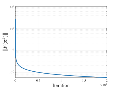
Figure 1: The infeasibility measured by $\ln\|F(\mathbf{x}^{k})\|$.

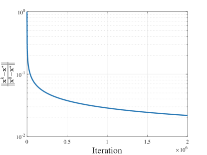
Figure 2: The optimality gap measured by $\ln\frac{\|\mathbf{x}^{k}-\mathbf{x}^{*}\|}{\|\mathbf{x}^{0}-\mathbf{x}^{*}\|}$.

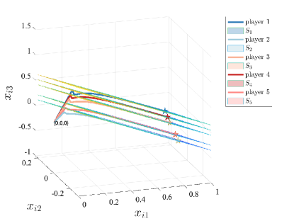
Figure 3: The decision trajectories of players generated by the algorithm. Each hyperplanes $S_{i}$ is a cut of the NE set $X^{*}$, while the star point corresponds with the optimal NE $\mathbf{x}^{*}$.

V Conclusion

We considered a monotone aggregative game, meanwhile the players coordinate to search a Nash equilibrium that minimizes the social cost. Based on a dynamical averaging tracking and Tikhonov regularization, we develop a distributed and single-timescale framework for seeking the optimal Nash equilibrium. Future works can be placed on various aspects, such as Nash games, complicated strategy sets, unbalanced directed graphs, and the relaxation of the strongly convex social cost to a convex or non-convex objective.

Proof of Lemma 3: (1) The proof is done in a similar fashion as that of [17, Lemma 4.5(a)]. According to the definition of $\mathbf{x}^{*}$ and $\mathbf{x}_{\eta_{k}}^{*}$, we have

$$F(\mathbf{x}^{*})^{T}(\mathbf{x}_{1}-\mathbf{x}^{*})\geq 0,~{}\forall\mathbf{x}_{1}\in\mathbb{R}^{mN},$$ (21)

$$\left(F(\mathbf{x}_{\eta_{k}}^{*})+\eta_{k}\nabla g(\mathbf{x}_{\eta_{k}}^{*})\right)^{T}(\mathbf{x}_{2}-\mathbf{x}_{\eta_{k}}^{*})\geq 0,~{}\forall\mathbf{x}_{2}\in\mathbb{R}^{mN}.$$ (22)

Let $\mathbf{x}_{1}=\mathbf{x}_{\eta_{k}}^{*},\mathbf{x}_{2}=\mathbf{x}^{*}$, and add (21) and (22) together, we obtain

$$\eta_{k}\nabla g(\mathbf{x}_{\eta_{k}}^{*})^{T}(\mathbf{x}^{*}-\mathbf{x}_{\eta_{k}}^{*})\geq(F(\mathbf{x}^{*})-F(\mathbf{x}_{\eta_{k}}^{*}))^{T}(\mathbf{x}^{*}-\mathbf{x}_{\eta_{k}}^{*}).$$

Recalling by Assumption 2 that the map $F(\mathbf{x})$ is monotone, we have $\nabla g(\mathbf{x}_{\eta_{k}}^{*})^{T}(\mathbf{x}^{*}-\mathbf{x}_{\eta_{k}}^{*})\geq 0$. From the strong convexity of $g$, we obtain that for all $k\geq 0$,

$$g(\mathbf{x}^{*}) \geq g(\mathbf{x}_{\eta_{k}}^{*})+\nabla g(\mathbf{x}_{\eta_{k}}^{*})^{T}(\mathbf{x}^{*}-\mathbf{x}_{\eta_{k}}^{*})+\frac{\mu_{g}}{2}\|\mathbf{x}^{*}-\mathbf{x}_{\eta_{k}}^{*})\|^{2}$$

$$\geq g(\mathbf{x}_{\eta_{k}}^{*}),$$ (23)

where we neglect the term $\frac{\mu_{g}}{2}\|\mathbf{x}^{*}-\mathbf{x}_{\eta_{k}}^{*}\|^{2}$. By Assumptions 2, 3 and Lemma 2, both $\mathbf{x}^{*}$ and $\mathbf{x}_{\eta_{k}}^{*}$ exist and are unique. Therefore, $g(\mathbf{x}_{\eta_{k}}^{*})$ is bounded. Further by the coercivity of $g$ (due to its strong convexity), the sequence $\{\mathbf{x}_{\eta_{k}}^{*}\}$ is bounded implying that it must have at least one limit point. Let $\{\mathbf{x}_{\eta_{k}}^{*}\}_{k\in\mathcal{K}}$ be an arbitrary subsequence such that $\lim_{k\rightarrow\infty,k\in\mathcal{K}}\mathbf{x}_{\eta_{k}}^{*}=\hat{\mathbf{x}}$. We now show that $\hat{\mathbf{x}}\in SOL(\mathbb{R}^{mN},F)$. Taking the limit on both sides of (22) with respect to the aforementioned subsequence and using the continuity of $F$ and $\nabla g$, we obtain that for all $\mathbf{y}\in\mathbb{R}^{mN}$, $(F(\hat{\mathbf{x}})+\lim_{k\rightarrow\infty,k\in\mathcal{K}}\eta_{k}\nabla g(\hat{\mathbf{x}}))^{T}(\mathbf{y}-\hat{\mathbf{x}})\geq 0$.

Because the sequence $\{\mathbf{x}_{\eta_{k}}^{*}\}$ is bounded, there exists a compact ball $\mathcal{X}\in\mathbb{R}^{mN}$ such that $\{\mathbf{x}_{\eta_{k}}^{*}\}_{k=0}^{\infty}\subseteq\mathcal{X}$. Combining with the continuity of $\nabla g$, we know that there exists a constant $C>0$ such that $\|\nabla g(\mathbf{x}_{\eta_{k}}^{*})\|\leq C$ for all $k\geq 0$. Recalling that $\lim_{k\rightarrow\infty}\eta_{k}=0$ by Assumption 5, we obtain that $F(\hat{\mathbf{x}})^{T}(\mathbf{y}-\hat{\mathbf{x}})\geq 0$ for all $\mathbf{y}\in\mathbb{R}^{mN}$, implying $\hat{\mathbf{x}}$ is a feasible solution to Problem ($P_{b}$). Next we show that $\hat{\mathbf{x}}$ is the optimal solution. From (23) we know that $g(\mathbf{x}^{*})\geq g(\lim_{k\rightarrow\infty,k\in\mathcal{K}}\mathbf{x}_{\eta_{k}}^{*})=g(\hat{\mathbf{x}})$. Hence, by the uniqueness of $\mathbf{x}^{*}$, all the limit points of $\{\mathbf{x}_{\eta_{k}}^{*}\}$ converge to $\mathbf{x}^{*}$ and this proof is completed.

(2) See the proof of [17, Lemma 4.5(b)]. $\hfill\blacksquare$

References

• [1] I. Caragiannis, M. Flammini, C. Kaklamanis, P. Kanellopoulos, and L. Moscardelli, “Tight bounds for selfish and greedy load balancing,” in International Colloquium on Automata, Languages, and Programming.   Springer, 2006, pp. 311–322.
• [2] S. R. Etesami, W. Saad, N. B. Mandayam, and H. V. Poor, “Stochastic games for the smart grid energy management with prospect prosumers,” IEEE Transactions on Automatic Control, vol. 63, no. 8, pp. 2327–2342, 2018.
• [3] A. Alcántara, J. Capitán, R. Cunha, and A. Ollero, “Optimal trajectory planning for cinematography with multiple unmanned aerial vehicles,” Robotics and Autonomous Systems, vol. 140, p. 103778, 2021.
• [4] S. Grammatico, “Dynamic control of agents playing aggregative games with coupling constraints,” IEEE Transactions on Automatic Control, vol. 62, no. 9, pp. 4537–4548, 2017.
• [5] C. Cenedese, F. Fabiani, M. Cucuzzella, J. M. Scherpen, M. Cao, and S. Grammatico, “Charging plug-in electric vehicles as a mixed-integer aggregative game,” in 2019 IEEE 58th Conference on Decision and Control (CDC).   IEEE, 2019, pp. 4904–4909.
• [6] M. Ye and G. Hu, “Game design and analysis for price-based demand response: An aggregate game approach,” IEEE transactions on cybernetics, vol. 47, no. 3, pp. 720–730, 2016.
• [7] F. Parise, S. Grammatico, B. Gentile, and J. Lygeros, “Distributed convergence to Nash equilibria in network and average aggregative games,” Automatica, vol. 117, p. 108959, 2020.
• [8] P. Zhou, W. Wei, K. Bian, D. O. Wu, Y. Hu, and Q. Wang, “Private and truthful aggregative game for large-scale spectrum sharing,” IEEE Journal on Selected Areas in Communications, vol. 35, no. 2, pp. 463–477, 2017.
• [9] R. Lahkar and S. Mukherjee, “Evolutionary implementation in a public goods game,” Journal of Economic Theory, vol. 181, pp. 423–460, 2019.
• [10] J. Koshal, A. Nedić, and U. V. Shanbhag, “Distributed algorithms for aggregative games on graphs,” Operations Research, vol. 64, no. 3, pp. 680–704, 2016.
• [11] S. Liang, P. Yi, and Y. Hong, “Distributed Nash equilibrium seeking for aggregative games with coupled constraints,” Automatica, vol. 85, pp. 179–185, 2017.
• [12] Y. Zhu, W. Yu, G. Wen, and G. Chen, “Distributed Nash equilibrium seeking in an aggregative game on a directed graph,” IEEE Transactions on Automatic Control, vol. 66, no. 6, pp. 2746–2753, 2020.
• [13] J. Lei, U. V. Shanbhag, and J. Chen, “Distributed computation of Nash equilibria for monotone aggregative games via iterative regularization,” in 2020 59th IEEE Conference on Decision and Control (CDC).   IEEE, 2020, pp. 2285–2290.
• [14] E. Koutsoupias and C. Papadimitriou, “Worst-case equilibria,” in Annual symposium on theoretical aspects of computer science.   Springer, 1999, pp. 404–413.
• [15] R. Mochaourab and E. Jorswieck, “Resource allocation in protected and shared bands: uniqueness and efficiency of Nash equilibria,” in Proceedings of the Fourth International ICST Conference on Performance Evaluation Methodologies and Tools, 2009, pp. 1–10.
• [16] D. Paccagnan, F. Parise, and J. Lygeros, “On the efficiency of Nash equilibria in aggregative charging games,” IEEE Control Systems Letters, vol. 2, no. 4, pp. 629–634, 2018.
• [17] H. D. Kaushik and F. Yousefian, “A method with convergence rates for optimization problems with variational inequality constraints,” SIAM Journal on Optimization, vol. 31, no. 3, pp. 2171–2198, 2021.
• [18] B. S. Pradelski and H. P. Young, “Learning efficient Nash equilibria in distributed systems,” Games and Economic behavior, vol. 75, no. 2, pp. 882–897, 2012.
• [19] J. R. Marden, H. P. Young, and L. Y. Pao, “Achieving pareto optimality through distributed learning,” SIAM Journal on Control and Optimization, vol. 52, no. 5, pp. 2753–2770, 2014.
• [20] A. Galeotti, B. Golub, and S. Goyal, “Targeting interventions in networks,” Econometrica, vol. 88, no. 6, pp. 2445–2471, 2020.
• [21] F. Facchinei and J.-S. Pang, “12 Nash equilibria: the variational approach,” Convex optimization in signal processing and communications, p. 443, 2010.
• [22] X. Li, L. Xie, and Y. Hong, “Distributed aggregative optimization over multi-agent networks,” IEEE Transactions on Automatic Control, pp. 1–1, 2021.
• [23] S. Pu and A. Nedić, “Distributed stochastic gradient tracking methods,” Mathematical Programming, vol. 187, no. 1, pp. 409–457, 2021.
• [24] B. T. Polyak, “Introduction to optimization. optimization software,” Inc., Publications Division, New York, vol. 1, p. 32, 1987.