Dark-siren Cosmology with Decihertz Gravitational-wave Detectors

Abstract

GW originated from mergers of stellar-mass binary black holes are considered as dark sirens in cosmology since they usually do not have electromagnetic counterparts. In order to study cosmos with these events, we not only need the luminosity distances extracted from GW signals, but also require the redshift information of sources via, say, matching GW sky localization with galaxy catalogs. Based on such a methodology, we explore how well decihertz GW detectors, DO-Optimal and DECIGO, can constrain cosmological parameters. Using Monte-Carlo simulated dark sirens, we find that DO-Optimal can constrain the Hubble parameter to ${\sigma_{H_{0}}}/{H_{0}}\,\lesssim 0.23\%$ when estimating $H_{0}$ alone, while DECIGO performs better by a factor of 5 with ${\sigma_{H_{0}}}/{H_{0}}\lesssim 0.043\%$. Such a good precision of $H_{0}$ will shed light on the $H_{0}$ tension. For multiple-parameter estimation, DECIGO can still reach a level of relative uncertainty smaller than $7\%$. The reason why decihertz detectors perform well is explained by their large numbers of SBBH GW events with good distance and angular resolution.

1 Introduction

The first direct detection of a gravitational wave (GW) event, namely GW150914, marked the beginning of GW astronomy [1]. According to the first half of the third observing run (O3a) detected by the Advanced Laser Interferometer Gravitational-wave Observatory (LIGO) and Advanced Virgo detectors [2], there are 39 GW candidate events detected so far [3]. Although most of them are not associated with electromagnetic (EM) observations, with the increasing number of detected GW events, a statistical study of the cosmic expansion is now possible [4]. For GW events with associated EM counterparts, because (i) GW signals can provide the luminosity distance of the sources, and (ii) the redshift information can be obtained from the EM observations, one can constrain cosmological parameters [5, 6, 7, 8, 9]. [5, 6, 7] Such GW events are called “standard sirens”. For example, the first binary neutron star merger GW170817 [2] and its numerous multi-band EM follow-ups [10, 11, 12, 13, 14, 15, 16, 17] became a milestone for the new era of multi-messenger astronomy. Based on these multi-messenger observations of GW170817, the Hubble parameter $H_{0}$ is constrained to be $H_{0}=70^{+12}_{-8}\,{\rm km\,s^{-1}\,Mpc^{-1}}$ (68$\%$ credible interval) [18].

By contrast, we call the GW events without EM counterparts “dark sirens” in the cosmological context. Although we lack the EM observations for these events, some statistic methods can still provide constraints on the cosmological parameters. In one of the dark-siren methods, a key point is that one can use a galaxy catalog. Fishbach et al. [19] first applied this method to GW170817 without regard to its EM follow-ups. Their results constrained $H_{0}$ to be $H_{0}=77^{+37}_{-18}\,{\rm km\,s^{-1}\,Mpc^{-1}}$. Recent studies have explored the prospects of the dark-siren cosmology using Bayesian framework with observations [4, 20] as well as simulated data [21, 22, 23, 24]. Extending earlier methods and criteria, in this work we discuss the constraints on the cosmological parameters with space-borne decihertz GW detectors.

In order to probe the cosmological parameters, GW signals should have high signal-to-noise ratio (SNR) and the inferred parameters should have good precision. Liu et al. [25] have shown that decihertz GW detectors could reach high distance resolution as well as high angular resolution, which are expected to provide accurate parameter estimations. Isoyama et al. [26] have also shown that the SNR for a GW150914-like binary black hole (BBH) merger event at decihertz waveband will be greater than that in the millihertz band. All of these indicate that space-borne decihertz GW detectors can provide crucial scientific value from the detection of SBBH merger events, especially in possessing the potential of measuring the Hubble parameter thus clarifying the Hubble tension.

In this work, we attempt to explore the constraints on the cosmological parameters with dark sirens by decihertz GW detectors. Specifically, we consider the DECihertz laser Interferometer Gravitational wave Observatory (DECIGO) [30], and Decihertz Observatories (DOs). DOs have two illustrative LISA-like designs, the more ambitious DO-Optimal and the less challenging DO-Conservative [32, 33], of which we choose DO-Optimal as a representative to study the capabilities of DOs on cosmological parameter constraints. The sensitive frequency band for DO-Optimal ranges from 0.01 Hz to 1 Hz, while DECIGO aims to detect GW sources in the frequency band between 0.1 Hz and 10 Hz. Although some estimations in the context of cosmology with DOs have been analyzed by Chen et al. [34], we consider a more realistic situation in our work, including the redshift error caused by the peculiar velocity [35, 36, 37] and the photo-z error caused by the photometric measurement [38]. For the luminosity distance errors, we further consider the bias of weak gravitational lensing [39].

The organization of this paper is as follows. We describe the methodology in Sec. 2. In Sec. 3, we illustrate the constraints on the cosmological parameters for DO-Optimal and DECIGO. Finally, we present our conclusions in Sec. 4.

2 Methodology

Assuming a flat $\rm\Lambda CDM$ universe throughout this work, the GW source’s luminosity distance $D_{\rm L}$ as a function of redshift $z$ can be written as

$${D_{\rm L}}=\frac{c(1+z)}{H_{0}}\int_{0}^{z}\frac{{\rm d}{z^{\prime}}}{\sqrt{{\rm\Omega_{M}}(1+z^{\prime})^{3}+\rm\Omega_{\Lambda}}}\,,$$ (1)

where $\rm\Omega_{M}$ is the present matter density fraction relative to the critical density, $\rm\Omega_{\Lambda}$ is the fractional density for present dark energy, $c$ is the speed of light, and $H_{0}$ is the Hubble constant. For a flat universe, we further have,

$$\rm\Omega_{\Lambda}+\Omega_{M}=1\,.$$ (2)

With known $D_{\rm L}$ and $z$ from many sources, $H_{0}$, $\rm\Omega_{M}$, and $\rm\Omega_{\Lambda}$ can be constrained using Eqs. (1) and (2). As noted in the Introduction, although we can get $D_{\rm L}$ from GW signals, the lack of EM follow-up observations means that we miss the redshift information for SBBH mergers [40]. However, the galaxy catalog can provide the redshift information for these dark sirens in a statistical way. Thus in this work, based on the simulated SBBH populations and related galaxy catalog, we constrain the cosmic parameters with the dark sirens that are to be detected by decihertz GW detectors.

Below we will introduce the strategy to generate SBBH population and galaxy catalog in Secs. 2.1 and 2.2, respectively. In Sec. 2.3 we describe a Bayesian framework to obtain the posterior probability distributions of cosmological parameters. We explain the uncertainty of the redshift and the luminosity distance in Sec. 2.4.

2.1 Populations of SBBHs

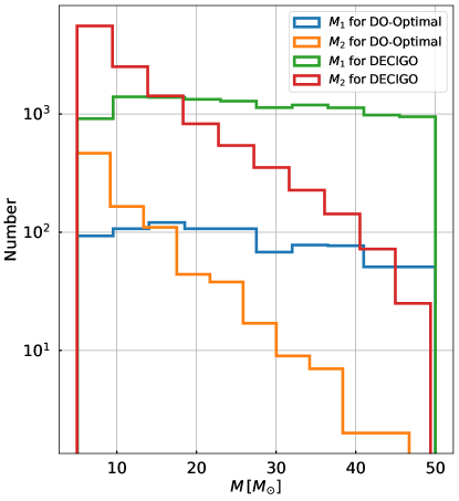
Figure 1: Mass histograms for detectable GW events in DO-Optimal and DECIGO during their 4-year mission lifetime.

Firstly, it is important to note that we artificially set $z_{\rm max}=1$ to be the upper detection limit in our work. This is because a larger $z$ tends to have a poorer localization accuracy, which will have less contribution to the cosmological parameter constraints. The realistic galaxy catalog is also less complete in the high-redshift regime. As for the mass generation of SBBHs, we use the flat-in-log mass model to generate the masses for each SBBH (see Fig. 1) [41]. The mass distribution for individual black hole (BH) is independently flat on the logarithmic scale as

$${\rm P}(M_{1},M_{2})\propto\frac{\rm 1}{M_{1}M_{2}}\,,$$ (3)

where ${\rm P}(M_{1},M_{2})$ is the probability that the component masses of SBBH are $M_{1}$ and $M_{2}$, respectively ($5M_{\odot}<M_{2}<M_{1}<50M_{\odot}$). Abbott et al. [41] estimated the merger rate $\rm\mathcal{R}=19^{+13}_{-8.2}\,Gpc^{-3}\,yr^{-1}$ under the assumption of a constant-redshift rate density and flat-in-log population. Conservatively, we set a 4-yr mission time ($T_{\rm m}$) for DO-Optimal and DECIGO. So the total number of SBBH merger events is $N_{\rm tot}=\frac{4}{3}\pi(D^{\rm max}_{\rm c})^{3}\times\mathcal{R}\times T_{\rm m}$, where $D^{\rm max}_{\rm c}$ is calculated using $z_{\rm max}$ via,

$${D_{\rm c}}=\frac{c}{H_{0}}\int_{0}^{z}\frac{{\rm d}z^{\prime}}{\sqrt{{\rm\Omega_{M}}(1+z^{\prime})^{3}+\rm\Omega_{\Lambda}}}\,.$$ (4)

And $N_{\rm tot}$ is around $1.2\times 10^{3}$.

The sky location of GW sources and their orbital angular momentum relative to the Earth direction are described by $\{\overline{\theta}_{\rm S},\overline{\phi}_{\rm S},\overline{\theta}_{\rm L},\overline{\phi}_{\rm L}\}$ in the ecliptic frame [25]. We randomly generate $N_{\rm tot}$ sets of $\{\overline{\theta}_{\rm S},\overline{\phi}_{\rm S},\overline{\theta}_{\rm L},\overline{\phi}_{\rm L}\}$ with ${\cos\,}\overline{\theta}_{\rm S},{\cos\,}\overline{\theta}_{\rm L}\in[-1,1]$ and $\overline{\phi}_{\rm S},\overline{\phi}_{\rm L}\in[0,2\pi)$. We then assign the GW events to host galaxies, and replace the sky location and distance with the value from the nearest galaxy as its host galaxy.

In order to generate luminosity distance and redshift of SBBHs, we assume here that galaxies are uniformly distributed in the comoving volume. So the probability density distribution within a spherical shell is given by

$${\rm P}(D_{\rm c})\propto{D_{\rm c}}^{2}\,,$$ (5)

where $D_{\rm c}\leq D^{\rm max}_{\rm c}$. The relation between luminosity distance ($D_{\rm L}$) and comoving distance ($D_{\rm c}$) is

$${D_{\rm L}}={(1+z)}{D_{\rm c}}\,.$$ (6)

We fix $H_{0}=67.8\,{\rm km\,s^{-1}\,Mpc^{-1}}$, $\Omega_{\rm M}=0.307$, and $\Omega_{\Lambda}=0.693$ to be the true values in our work, which is derived from the $Planck$ observations [29, 42].

2.2 Populations of host galaxies

Consistent with Liu et al. [25], we use the IMRPhenomD model to produce the simulated GW signals [43, 44]. The waveform is a function of the following physical parameters,

$${\overrightarrow{\vartheta}}=\{\mathcal{M},{D}_{\rm L},\chi_{1},\chi_{2},t_{\rm c},\phi_{\rm c},\eta\}\,,$$ (7)

where $\mathcal{M}=(M_{1}+M_{2}){\eta}^{3/5}$ is the chirp mass with the symmetric mass ratio $\eta=M_{1}M_{2}/{(M_{1}+M_{2})^{2}}$. $t_{\rm c},\phi_{\rm c}$ are respectively the time and phase at coalescence and $\chi_{1},\chi_{2}$ are the dimensionless BH spins. Without losing generality, we choose $t_{\rm c}=0,\phi_{\rm c}=0,\chi_{1}=0,\chi_{2}=0$ as fiducial values for each SBBH [3]. And the relationship between the frequency-domain GW signal $\widetilde{h}(f)$ in the detector and the incident cross and plus GW signals is

$${\widetilde{h}(f)=F^{+}(f)\widetilde{h}_{+}(f)+F^{\times}(f)\widetilde{h}_{\times}(f)}\,,$$ (8)

where $F^{+}(f),F^{\times}(f)$ are frequency-dependent detector pattern functions and $\widetilde{h}_{+}(f),\widetilde{h}_{\times}(f)$ are the source GW waveform provided by the IMRPhenomD. Following Liu et al. [25], we use the Fisher information matrix (FIM) to perform parameter estimations for SBBH events with SNR larger than 10. We obtain the angular resolution $\rm\Delta\Omega$ and the luminosity distance resolution $\Delta D_{\rm L}$ of the SBBH mergers. Note that the definition of $\rm\Delta\Omega$ is

$${\rm\Delta\Omega}=2\pi\sqrt{{\left(\Delta\overline{\phi}_{\rm S}\Delta{\rm cos}\,\overline{\theta}_{\rm S}\right)}^{2}-{\left\langle\delta\overline{\phi}_{\rm S}\delta{\rm cos}\,\overline{\theta}_{\rm S}\right\rangle}^{2}}\,,$$ (9)

where $\Delta\overline{\phi}_{\rm S}$ and $\Delta{\rm cos}\,\overline{\theta}_{\rm S}$ are the root mean square errors of $\overline{\phi}_{\rm S}$ and ${\rm cos}\,\overline{\theta}_{\rm S}$, respectively; $\left\langle\delta\overline{\phi}_{\rm S}\delta{\rm cos}\,\overline{\theta}_{\rm S}\right\rangle$ is the covariance of $\overline{\phi}_{\rm S}$ and ${\rm cos}\,\overline{\theta}_{\rm S}$. More details can be seen in Liu et al. [25]. Then we simulate the galaxy catalog with the assumption that such a galaxy catalog is completed within $z_{\rm max}=1$. We use flat priors for $H_{0}\in[10,120]\,{\rm km\,s^{-1}\,Mpc^{-1}}$, ${\rm\Omega_{M}}\in[0.1,0.5]$, and ${\rm\Omega_{\Lambda}}\in[0.5,0.9]$. Combining priors and $\Delta D_{\rm L}$, we obtain the upper (lower) limit $z^{\rm upp}$ ($z^{\rm low}$) of each SBBH merger. We also obtain the upper and lower limits of the luminosity distance, $D_{\rm L}^{\rm low}$ and $D_{\rm L}^{\rm upp}$, and the comoving distance, $D_{\rm c}^{\rm low}$ and $D_{\rm c}^{\rm upp}$. So the comoving volumetric error $\Delta V_{\rm c}$ of each GW source including the host galaxy and other candidate galaxies is given by

$${\Delta V_{\rm c}}\approx\frac{\rm 1}{\rm 3}{\rm\Delta\Omega}\left[{\big{(}{D_{\rm c}^{\rm upp}}\big{)}^{3}-\big{(}{D_{\rm c}^{\rm low}}\big{)}^{3}}\right]\,.$$ (10)

It is the volume of the frustum of a comoving cone. Given that the average number density of the Milky-Way-like galaxy is $\sim 0.01\,\rm Mpc^{-3}$ [45, 46], the expected number of possible host galaxies in each $\Delta V_{\rm c}$ can be roughly estimated as

$${\bar{N}_{\rm gal}}=0.01{\Delta V_{\rm c}}\,{\rm Mpc}^{-3}\,.$$ (11)

Note that the definition of possible host galaxies here is from the perspective of actual detection, and it includes the host galaxy and other candidate galaxies. We obtain the total number of galaxies $N_{\rm gal}$ from a Poisson distribution with its mean value $\bar{N}_{\rm gal}$. The number of other candidate galaxies in $\Delta V_{\rm c}$ is $N_{\rm can}=N_{\rm gal}-1$. For the mergers with $\bar{N}_{\rm gal}<1$, we can directly set $N_{\rm gal}=1$. We generate the redshift of other candidate galaxies in the same way as SBBHs. In reality, galaxies are clustered on small scales rather than uniformly distributed as assumed here [47, 48, 49]. Clustered galaxies will provide more informative redshift distribution, improving the constraints on cosmological parameters. Thus we are conservative in this aspect.

As we will see later in Sec. 2.3, we consider different weights for each galaxy in each $\Delta V_{\rm c}$ based on their position and masses. Before that, we first discuss how we allocate the position and mass to each galaxy. For the position, we get the uncertainty $\{\rm\Delta\overline{\theta}_{\rm S},\Delta\overline{\phi}_{\rm S}\}$ by the FIM method. We can obtain an ellipse projected on the tangent plane of the celestial sphere, and it is centered on the host galaxy. The principal axes of this ellipse are $\rm 3\Delta\overline{\theta}_{\rm S}$ and $\rm 3\Delta\overline{\phi}_{\rm S}$. In this ellipse, we randomly simulate galaxies to provide different position information for later use.

We use a galaxy’s total stellar mass as a proxy for its mass, and assume other candidate galaxies’ masses directly follow the stellar mass function (SMF) in Kelvin et al. [50]. Assuming that the formation rate of SBBHs is uniform for all galaxies, we expect that the more massive the galaxy is, the more likely it is the host galaxy of the SBBH [19]. Thus, in order to highlight the contribution of the host galaxy, we regard the mass distribution of the host galaxy as the distribution of $\rho{M}$, where $\rho$ is the number density of galaxy and ${M}$ is the galaxy mass. The values of $\rho$ and ${M}$ are obtained from the SMF. Following this “mass-weighted” SMF distribution, we generate a statistically larger mass for the host galaxy than the candidate galaxies’ masses generated from the SMF. Note that this treatment is crude but reasonable. At this point, we have generated the masses of all the galaxies, and this is different from Zhu et al. [23], and Chen and Amaro-Seoane [51].

In addition to generating host galaxy populations according to the above method, another realistic simulated galaxy catalog will also be considered in Sec. 3.3. We will present more results in later sections.

2.3 Bayesian framework

We use the Bayesian framework to derive the precision of the cosmological parameters from our simulated dark sirens and related galaxy catalogs. In our notation, a set of GW data $\mathcal{D}_{\rm GW}\equiv\{\mathcal{D}_{\rm GW}^{1},...,\mathcal{D}_{\rm GW}^{i},...,\mathcal{D}_{\rm GW}^{N_{\rm tot}}\}$ includes $N_{\rm tot}$ GW events, characterized by the luminosity distance $D_{\rm L}$, the position $\{\rm\overline{\theta}_{\rm S},\overline{\phi}_{\rm S}\}$ and so on. The posterior probability distribution for the cosmological parameters can be estimated by

$${\rm P}(\mathcal{H}|\mathcal{D}_{\rm GW},I)\propto{{\rm P}(\mathcal{H}|I)}{{\rm P}(\mathcal{D}_{\rm GW}|\mathcal{H},I)}\,,$$ (12)

where $\mathcal{H}\equiv\{H_{0},{\rm\Omega_{M},\Omega_{\Lambda}}\}$, ${\rm P}(\mathcal{H}|I)$ is the prior probability distribution of $\mathcal{H}$, and $I$ represents all the related background information. In addition, we use ${{D}_{\rm L}^{i}}$ to represent the true luminosity distance of the $i$-${\rm th}$ host galaxy. We assume that it is equal to the luminosity distance of the SBBH merger event. The second term in the right hand side of Eq. (12) is called the likelihood function, and it can be derived as

$${\rm P}(\mathcal{D}_{\rm GW}|\mathcal{H},{I})=\prod_{i=1}^{N_{\rm tot}}{{\rm P}(\mathcal{D}_{\rm GW}^{i}|\mathcal{H},{I})}\,.$$ (13)

For each merger event, ${\rm P}(\mathcal{D}_{\rm GW}^{i}|\mathcal{H},{I})$ can be expressed as

$${\rm P}(\mathcal{D}_{\rm GW}^{i}|\mathcal{H},{I})= \int{{\rm d}{D}_{\rm L}}\int{{\rm d}z}\int{{\rm d}M}\int{{\rm d}\Omega}$$ (14)

$$\times{{\rm P}(\mathcal{D}_{\rm GW}^{i}|{{D}_{\rm L}},{z,{M},}\Omega,\mathcal{H},{I})}$$

$$\times{{\rm P}({z,{M}},\Omega|\mathcal{H},{I})}$$

$$\times{{\rm P}({{D}_{\rm L}}|{z,{M}},\Omega,\mathcal{H},I)}\,,$$

where $M$ is the mass of each possible host galaxy. Adopting Gaussian noise for GW signals [52], ${\rm P}(\mathcal{D}_{\rm GW}^{i}|\mathcal{H},I)$ is assumed to follow a Gaussian distribution $\mathcal{N}\big{[}\widetilde{{D}}_{\rm L}^{i},(\sigma_{{D}_{\rm L}^{i},j})^{2}\big{]}$, where $\widetilde{{D}}_{\rm L}^{i}$ represents the detected luminosity distance; $\sigma_{{D}_{\rm L}^{i},j}$ is the standard deviation including the error of the redshift and the luminosity distance. We assume that $\widetilde{{D}}_{\rm L}^{i}$ follows $\widetilde{{D}}_{\rm L}^{i}\sim\mathcal{N}\big{[}{D}_{\rm L}^{i},{(\sigma_{D_{\rm L}}^{\rm GW})}^{2}\big{]}$. Note that $\sigma_{D_{\rm L}}^{\rm GW}$ here is the bias of the luminosity distance obtained from the GW signals alone, and it is one of the components of $\sigma_{{D}_{\rm L}^{i},j}$, to be discussed later in the next subsection. The subscript $j$ represents the $j$-th galaxy within the error volume for the $i$-th merger event. In our notation, $j=1$ represents the host galaxy and there are $N_{\rm can}^{i}$ other candidate galaxies in the $i$-th error volume. So, the redshift information in each error volume is $\big{\{}{z}_{i,1},\cdots,{z}_{i,j},\cdots,{z}_{i,N_{\rm gal}^{i}}\big{\}}$. In addition, we assume a $\rm\delta-$function for ${{\rm P}({{D}_{\rm L}}|{z,M},\Omega,\mathcal{H},I)}$ via

$${{\rm P}({{D}_{\rm L}}|{z,M},\Omega,\mathcal{H},I)}=\delta\big{(}{D}_{\rm L}-{D}_{\rm L}(z,\mathcal{H})\big{)}\,,$$ (15)

where ${D}_{\rm L}(z,\mathcal{H})$ is the transformed luminosity distance of $z$ with the cosmology parameter $\mathcal{H}$ in Eq. (1).

For ${{\rm P}({z,M},\Omega|\mathcal{H},{I})}$, we express it as

$${\rm P}({z,M},\Omega|\mathcal{H},{I})\propto \sum_{j=1}^{N_{\rm gal}^{i}}\Big{[}\delta({z}-{z}_{i,j})\times{W_{\rm pos}^{i,j}(\Omega)}$$ (16)

$$\times{W_{\rm mass}^{i,j}(M)}\Big{]}\,,$$

where $\delta({z}-{z}_{i,j})$ means that the weight from the redshift of each galaxy is the same. $W_{\rm pos}^{i,j}(\Omega)$ and $W_{\rm mass}^{i,j}(M)$ represent the weights from the position and the mass of each galaxy, respectively. We could get the covariance matrix $\Xi_{\overline{\theta}_{\rm S},\overline{\phi}_{\rm S}}^{i}$ of sky location from each merger event by the FIM method. The positional weight is obtained as

$${f}_{\rm pos}(\overline{\theta}_{\rm S}^{i,j},\overline{\phi}_{\rm S}^{i,j})\propto {\rm exp}\bigg{[}-\frac{1}{2}\big{(}\overline{\theta}_{\rm S}^{i,j}-\overline{\theta}_{\rm S}^{i,1},\overline{\phi}_{\rm S}^{i,j}-\overline{\phi}_{\rm S}^{i,1}\big{)}$$ (17)

$${\Xi_{\overline{\theta}_{\rm S},\overline{\phi}_{\rm S}}^{i}\big{(}\overline{\theta}_{\rm S}^{i,j}-\overline{\theta}_{\rm S}^{i,1},\overline{\phi}_{\rm S}^{i,j}-\overline{\phi}_{\rm S}^{i,1}\big{)}^{\rm T}\bigg{]}}\,,$$

$${W_{\rm pos}^{i,j}(\Omega)}\propto {f}_{\rm pos}(\overline{\theta}_{\rm S},\overline{\phi}_{\rm S})\times\delta(\overline{\theta}_{\rm S}-\overline{\theta}_{\rm S}^{i,j})$$ (18)

$$\times\delta(\overline{\phi}_{\rm S}-\overline{\phi}_{\rm S}^{i,j})\,,$$

where $\{\overline{\theta}_{\rm S}^{i,j},\overline{\phi}_{\rm S}^{i,j}\}$ represent the sky location of each galaxy in $\Delta V_{\rm c}$; ${f}_{\rm pos}(\overline{\theta}_{\rm S}^{i,j},\overline{\phi}_{\rm S}^{i,j})$ represents the probability density at the sky location. As mentioned in Sec. 2.2, $W_{\rm mass}^{i,j}(M)$ is defined as

$${W_{\rm mass}^{i,j}(M)}\propto M\times\delta({M}-{M}_{i,j})\,.$$ (19)

From Eqs. (13–19), we can derive the likelihood for all the GW events as

$${\rm P} (\mathcal{D}_{\rm GW}|\mathcal{H},{\rm I})\propto\prod_{i=1}^{N_{\rm tot}}\bigg{\{}\sum_{j=1}^{N_{\rm gal}^{i}}\Big{[}{M}_{i,j}\times{f}_{\rm pos}(\overline{\theta}_{\rm S}^{i,j},\overline{\phi}_{\rm S}^{i,j})$$ (20)

$$\times{\frac{1}{\sqrt{2\pi}{{\sigma_{{D}_{\rm L}^{i},j}}}}{\rm exp}\Big{(}-\frac{{\big{(}{D}_{\rm L}({z}_{i,j},\mathcal{H})-\widetilde{{D}}_{\rm L}^{i}\big{)}}^{2}}{2({\sigma_{{D}_{\rm L}^{i},j}})^{2}}\Big{)}}\Big{]}\bigg{\}}\,.$$

According to Eqs. (12–20), we calculate the posterior probability distributions of the cosmological parameters $\mathcal{H}$. Note that the cosmological parameter error might originate from the EM selection effect. The GW selection effect is not considered in this work because the constraints mainly depend on the nearest GW events, which have large SNRs and well localization or even the best localization. The bias introduced by the GW selection effect is negligible for these events. Taking DO-Optimal as an example, from Table 2, only about $10\%$ of the GW events are well-localized, and about $80\%$ of these well-localized events have large SNRs (SNR>50). This means that the majority of the sources used for the GW cosmology study are high SNR events, therefore will not suffer from GW selection bias. Besides, Fig. 2(a) shows that DO-Optimal can detect well-localized events with $z\lesssim 0.5$. Therefore, we argue that the GW selection effect will not introduce GW bias too much in the constraints of the cosmological parameters. For the influence of the EM selection effect, more details will be discussed in Sec. 3.3 with the simulated galaxy catalog.

We use the method of Markov Chain Monte Carlo (MCMC) to obtain the parameter estimations and perform a series of MCMC studies with emcee, a Python package that implements an affine-invariant MCMC ensemble sampler [53, 54].

2.4 Uncertainty of redshift and luminosity distance

For the luminosity distance, we consider the following two possible errors. (i) We use a fitting function in Hirata et al. [39] to estimate the error from the weak lensing effects, which is given by

$${\sigma_{D_{\rm L}}^{\rm lens}(z)}={{\rm C}\;\bigg{[}\frac{1-(1+z)^{-\beta}}{\beta}\bigg{]}^{\alpha}\;D_{\rm L}}\,,$$ (21)

where $\rm C=0.066$, $\beta=0.25$, and $\alpha=1.8$. (ii) As mentioned in Sec. 2.2, we can get $\Delta D_{\rm L}$ through FIM for each GW event. So the error from the GW measurements could be expressed as

$${\sigma_{D_{\rm L}}^{\rm GW}(z)}={\Delta D_{\rm L}}\,.$$ (22)

To adequately describe the uncertainty of the redshift, we consider two kinds of errors and then transform both uncertainties into the errors on the luminosity distance. (i) According to Ilbert et al. [38], the uncertainty from the photometric redshift is given by

$${\sigma_{z}^{\rm photo}(z)}={0.008(1+z)}\,.$$ (23)

Then based on Kocsis et al. [36] and the chain rule, we derive

$${\sigma_{D_{\rm L}}^{\rm photo}(z)} =\frac{\partial{D_{\rm L}(z)}}{\partial{z}}{\sigma_{z}^{\rm photo}(z)}\,.$$ (24)

(ii) Gordon et al. [35], Kocsis et al. [36], and He [37] estimated the redshift error from the peculiar velocity of galaxies by

$${\sigma_{D_{\rm L}}^{\rm pv}(z)}={\Big{[}1-\frac{c(1+z)^{2}}{H(z)D_{\rm L}}\Big{]}\;\frac{\sqrt{\langle v^{2}\rangle}}{c}\;D_{\rm L}}\,,$$ (25)

$${H(z)}=H_{0}{\sqrt{\Omega_{\rm M}(1+z)^{3}+{\rm\Omega_{\Lambda}}}}\,,$$ (26)

where $\sqrt{\langle v^{2}\rangle}=500\;\rm km/s$ is the root mean square peculiar velocity of the galaxy with respect to the Hubble flow [23, 37].

Combining all the errors mentioned above, the total uncertainty of the luminosity distance of the $j$-th possible host galaxies corresponding to the $i$-th GW event is expressed as

$${\sigma_{{D}_{\rm L}^{i},j}({z}_{i,j})}={\sqrt{{(\sigma_{D_{\rm L}}^{\rm photo})}^{2}+{(\sigma_{D_{\rm L}}^{\rm pv})}^{2}+{(\sigma_{D_{\rm L}}^{\rm lens})}^{2}+{(\sigma_{D_{\rm L}}^{\rm GW})}^{2}}}\,.$$ (27)

3 Results

In this section, we compare the constraints on the cosmology parameters with dark sirens between DO-Optimal and DECIGO. Sec. 3.1 gives results for a single parameter $H_{0}$, and Sec. 3.2 gives results for multiple parameters. Sec. 3.3 gives results for parameters by using a realistic simulated galaxy catalog.

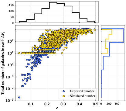
(a) DO-Optimal

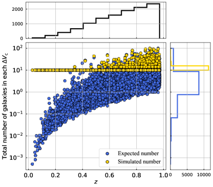
(b) DECIGO

Figure 2: The expected number (blue) and the simulated number (yellow) of galaxies in each $\Delta V_{\rm c}$ are given in dots, and the detectable merger events are summarized with histograms.

3.1 Estimations for a single parameter $H_{0}$

As mentioned in Sec. 2.3, the luminosity distance of the $i$-th simulated merger event is ${D}_{\rm L}^{i}$. The corresponding redshifts of possible host galaxies are $\big{\{}{z}_{i,1},\cdots,{z}_{i,j},\cdots,{z}_{i,{N}_{\rm gal}^{i}}\big{\}}$. By using Eq. (1), we can get each ${H}_{0}^{ij}$ with ${D}_{\rm L}^{i}$ and ${z}_{i,j}$. As noted in Sec. 2.4, we have transformed the redshift uncertainty to the luminosity uncertainty, and then we calculate the total uncertainty $\sigma_{{H}_{0}^{ij}}^{\rm tot}={\lvert{\partial{H_{f}(z)}}/{\partial{D_{\rm L}}}\rvert\cdot\lvert\sigma_{{D}_{\rm L}^{i},j}\rvert}$ of ${H}_{0}^{ij}$ by using Eq. (27) and the chain rule. Note that $H_{f}(z)$ is derived by Eq. (1). The likelihood of ${H}_{0}$ constrained from the $i$-th event can thus be expressed as

$${\rm P}(\mathcal{D}_{\rm GW}^{i} |{H_{0},I})\propto\sum_{j=1}^{{N}_{\rm gal}^{i}}\bigg{[}{M}_{i,j}\times{f}_{\rm pos}(\overline{\theta}_{\rm S}^{i,j},\overline{\phi}_{\rm S}^{i,j})$$ (28)

$$\times{\frac{1}{\sqrt{2\pi}{\sigma_{{H}_{0}^{ij}}^{\rm tot}}}{\rm exp}\Big{(}-\frac{({H}_{0}-{H}_{0}^{ij})^{2}}{2({\sigma_{{H}_{0}^{ij}}^{\rm tot}})^{2}}\Big{)}}\bigg{]}\,.$$

Finally, we calculate the likelihood of ${H}_{0}$ constrained by all simulated merger events with Eq. (13). Note that for simplicity, we select the well-localized simulated merger events with the total number of galaxies in $\Delta V_{\rm c}$ less than 100, i.e. ${N}_{\rm gal}^{i}\leq 100$. As these events are most constraining, this choice, while speeding up our calculation enormously, will not change our result in a significant way.

We show in Fig. 2 the relationship between the total number of simulated galaxies for each merger event and their redshifts. We find that DO-Optimal can detect well-localized SBBH merger events with $z\lesssim 0.5$, while the redshift can be much larger for DECIGO, reaching $z\sim 1$. We also see that DECIGO has a better performance not only on the total number of the merger events but also on the “best-localized” events. The best-localized events are defined that there is only one galaxy within $\Delta V_{\rm c}$. As shown in Fig. 3, the excellent performance of DECIGO can be explained by its better distance and angular resolution than DO-Optimal. Fig. 3 also shows that, in our samples, DECIGO’s minimum values for the distance relative error and angular resolution can reach $\sim 10^{-6}$ and $\sim 10^{-6}\,{\rm arcmin}^{2}$, respectively.

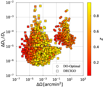
Figure 3: The relative uncertainty on the luminosity distance and angular resolution for DO-Optimal (circles) and DECIGO (squares) in our simulated samples.

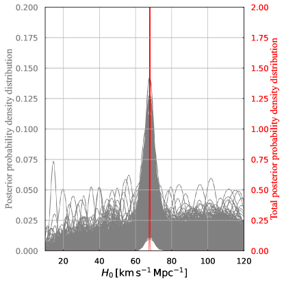
(a) DO-Optimal

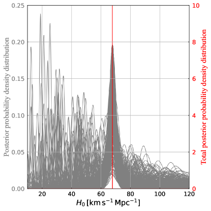
(b) DECIGO

Figure 4: The posterior probability density distributions of ${H}_{0}$ for each GW event (gray) and the total posterior probability density distribution (red) for DO-Optimal (left) and DECIGO (right).

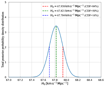
(a) DO-Optimal

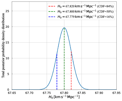
(b) DECIGO

Figure 5: Posterior probability density distributions of ${H}_{0}$ with a 68% confidence level from combining all events in DO-Optimal (left) and DECIGO (right).

Detector	1-parameter	2-parameter		3-parameter
	$\frac{\sigma_{H_{0}}}{H_{0}}(\%)$	$\frac{\sigma_{H_{0}}}{H_{0}}(\%)$	$\frac{\sigma_{\Omega_{\rm M}}}{\Omega_{\rm M}}(\%)$	$\frac{\sigma_{H_{0}}}{H_{0}}(\%)$	$\frac{\sigma_{\Omega_{\rm M}}}{\Omega_{\rm M}}(\%)$	$\frac{\sigma_{\Omega_{\Lambda}}}{\Omega_{\Lambda}}(\%)$
DO-Optimal	0.17	1.8	44	1.7	86	33
DECIGO	0.029	0.14	0.98	0.42	3.3	5.1
Using a realistic simulated galaxy catalog from the TAO
DECIGO	0.032	0.18	1.3	0.47	4.6	6.6

Table 1: Constraints on the cosmological parameters with DO-Optimal and DECIGO.

Detector	$N_{\rm tot}$			${N}_{\rm gal}\leq 100$ (well-localized)		SNR>10
	11696					${N}_{\rm gal}\leq 10$	${N}_{\rm gal}\leq 3$	${N}_{\rm gal}=1$ (best-localized)
	SNR>10	SNR>50	SNR>100	SNR>10	SNR>50
DO-Optimal	11694	8210	3741	860	719	329	194	133
DECIGO	11696	11696	11693	11689	11689	11626	11491	11120
Using a realistic simulated galaxy catalog from the TAO
DECIGO	$N_{\rm sel}$			11293	11293	10396	8584	5611
	11396
	SNR>10	SNR>50	SNR>100
	11396	11396	11394

Table 2: The number of GW events with different SNR thresholds and ${N}_{\rm gal}$.

We can see in Fig. 4 that there are multiple peaks on the posterior probability density distributions for each merger event, given by gray lines. For each gray line, among the peaks it has, there is always a peak near the true value, $H_{0}=67.8\,{\rm km\,s^{-1}\,Mpc^{-1}}$ in our injection. In addition, the well-localized GW events $({N}_{\rm gal}^{i}\leq 100)$ tend to have better constraints on $H_{0}$, and have made a major contribution. For more comparisons between DO-Optimal and DECIGO, we show the $1$-$\sigma$ range of the combined posterior probability density distributions in Fig. 5. The given values of cumulative distribution function (CDF) are the medians, along with its $16\%$ and $84\%$ quantiles. We can see that the relative uncertainties of $H_{0}$ for DO-Optimal and DECIGO are about $0.17\%$ and $0.029\%$, respectively. Therefore, both DO-Optimal and DECIGO can constrain $H_{0}$ quite well. Between them, DECIGO performs even better. It is not only related to DECIGO’s excellent positioning capability but also its larger number of detectable merger events (cf. Figs. 2–3 and Table 2).

3.2 Estimations for multiple parameters

For simplicity, we uniformly select GW events with ${N}_{\rm gal}^{i}\leq 3$. We have verified with ${N}_{\rm gal}^{i}\leq 10$ that the results are consistent. Thus we only illustrate our results with ${N}_{\rm gal}^{i}\leq 3$ in this subsection.

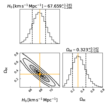
(a) DO-Optimal

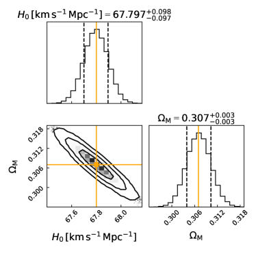
(b) DECIGO

Figure 6: Two-parameter estimations for $\big{\{}H_{0},\Omega_{\rm M}\big{\}}$ with DO-Optimal (left) and DECIGO (right).

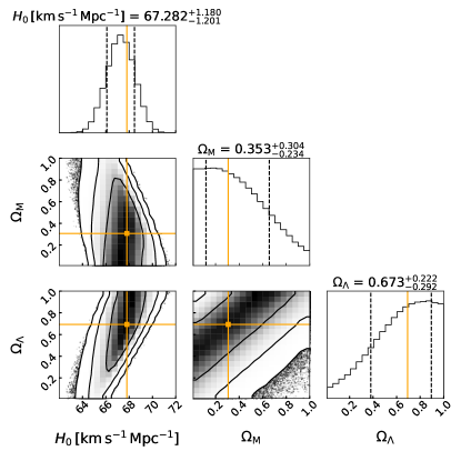
(a) DO-Optimal

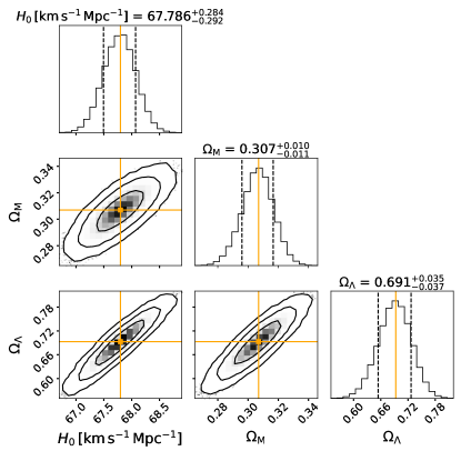
(b) DECIGO

Figure 7: Three-parameter estimations for $\big{\{}H_{0},{\rm\Omega_{M},\Omega_{\Lambda}}\big{\}}$ with DO-Optimal (left) and DECIGO (right).

We first consider two parameters $\big{\{}H_{0},\Omega_{\rm M}\big{\}}$ with $\Omega_{\Lambda}=1-\Omega_{\rm M}$ in Eq. (2). We find in Fig. 6 that DECIGO has better constraints on $\big{\{}H_{0},\Omega_{\rm M}\big{\}}$ with relative errors of $\sim 0.14\%$ and $\sim 0.98\%$, respectively. In contrast, DO-Optimal can constrain $H_{0}$ with a relative error of $\sim 1.8\%$, while it performs worse on $\Omega_{\rm M}$ with a relative error of $\sim 44\%$.

In addition to the results above, we further consider treating $\Omega_{\Lambda}$ as an independent variable and then performing parameter estimations on $\mathcal{H}$ with three parameters. Fig. 7(a) shows the estimation results for the two detectors. We see in Fig. 7(a) that DO-Optimal can constrain $H_{0}$ well with a relative error of $\sim 1.7\%$, but has basically no constraints on $\Omega_{\rm M}$ and $\Omega_{\Lambda}$ with relative errors reaching $\sim 86\%$ and $\sim 33\%$, respectively. This can be explained well by the low localization accuracy of the high-redshift events for DO-Optimal. In contrast, DECIGO still has a much better performance on the parameter estimations, as shown in Fig. 7(b). The relative errors of $\big{\{}H_{0},{\rm\Omega_{M},\Omega_{\Lambda}}\big{\}}$ can reach $\sim 0.42\%$, $\sim 3.3\%$, and $\sim 5.1\%$, respectively.

Comparing the 2-parameter and 3-parameter constraints from the two detectors, we conclude that DECIGO behaves much better than DO-Optimal. Both detectors can constrain $H_{0}$ well, while for $\Omega_{\rm M}$ and $\Omega_{\Lambda}$, only DECIGO can reach a significant result with relative errors $\leq 6\%$. The differences between DECIGO and DO-Optimal are mainly due to the different localization capabilities, especially for the high-redshift events. DECIGO can detect well-localized merger events even at $z=1$, significantly improving the constraints. Moreover, $\Omega_{\rm M}$ and $\Omega_{\Lambda}$ dominate in the high-redshift regime based on Eq. (1), which determines that it is hard for DO-Optimal to give more precise measurements of $\Omega_{\rm M}$ and $\Omega_{\Lambda}$.

It is worth noting that for the same detector, the single parameter constraints can be much better than the results of the multiple parameters. The increase in relative error can be explained by the degrees of freedom. We summarize our marginalized constraints in Table 1 and the number of GW events under different cutoffs in calculations in Table 2.

3.3 Estimations with a realistic simulated galaxy catalog

We adopt the MultiDark Planck (MDPL) cosmological simulation [55] and the Semi-Analytic Galaxy Evolution (SAGE) model [56] from the Theoretical Astrophysical Observatory (TAO) to generate a realistic simulated galaxy catalog. The MDPL simulation assumes a Planck cosmology [42], and the TAO is a publicly available codebase that runs on the dark matter halo trees of a cosmological N-body simulation. In addition to the locations of the galaxies, the MDPL also provide the luminosity information of the galaxies according to Croton et al. [56], Conroy and Wechsler [57].

All the information obtained from the simulated catalog includes luminosity distance, redshift, mass, location, and apparent magnitude in the K-band. Then we adopt a mass-weighted random selection of $N_{\rm tot}$ host galaxies. To be more realistic, we also simulate the EM selection effect. Following Zhu et al. [23], the probability that a galaxy with luminosity $\mathcal{L}$ (in the unit of sun’s luminosity) can be observed is defined as

$${\mathcal{P}({\rm lg}\mathcal{L})=\int_{{\rm lg}\mathcal{L}_{\rm limit}}^{\infty}\mathcal{N}\big{[}\mathcal{L},(\sigma_{{\rm lg}\mathcal{L}})^{2}\big{]}\,d\mathcal{L}^{\prime}}\,,$$ (29)

where ${\rm lg}\mathcal{L}_{\rm limit}=\frac{{\rm m}_{\odot}-{\rm m_{\rm limit}}-5}{2.5}+2{\rm lg}\big{(}\frac{D_{\rm L}}{1{\rm pc}}\big{)}$ with the absolute magnitude of the sun ${\rm m}_{\odot}=+4.8\,{\rm mag}$ and the limiting apparent magnitude ${\rm m_{\rm limit}}=+24\,{\rm mag}$. We adopt the measurement error of limiting luminosity $\sigma_{{\rm lg}\mathcal{L}}=0.04$ [23, 58, 59]. As shown in Table 2, the total number of SBBH merger events is reduced to $N_{\rm sel}=11396$ due to the EM selection effect. Considering that the calculation is very time-consuming, we only use DECIGO as a representative to constrain the cosmological parameters and compare them with the previous results in Sec. 3.1 and 3.2.

We adopt the same method as in Sec. 2.3 to constrain the cosmological parameters. Note that when we calculate the position weights of galaxies in each $\Delta V_{\rm c}$, to be more realistic, we have added a random bias to the location of the error volume’s center relative to the host galaxy. The results are shown in Fig. 8 and summarized in Table 1. We find that even considering the EM selection effect with a realistic simulated galaxy catalog, DECIGO can also constrain the cosmological parameters well. The relative uncertainties of $H_{0}$ for DECIGO is $\sim 0.032\%$; $\big{\{}H_{0},{\rm\Omega_{M}}\big{\}}$ is about $\sim 0.18\%$ and $\sim 1.3\%$. For the 3-parameter $\big{\{}H_{0},{\rm\Omega_{M},\Omega_{\Lambda}}\big{\}}$ estimations, DECIGO can reach $\sim 0.47\%$, $\sim 4.6\%$, and $\sim 6.6\%$, respectively. In addition, we find that DECIGO’s constraints on cosmological parameters are consistent (a little worse) with the previous results in Sec. 3.1 and 3.2, which indicates that the EM selection effect has little influence on the results of DECIGO’s constraints. Besides, 11396 GW events with SNR>10 also provide a lot of best-localized events (5611 GW events).

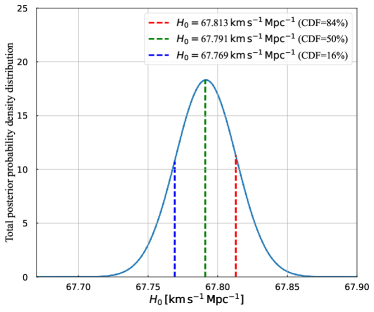
(a) Estimation for $\big{\{}H_{0}\big{\}}$

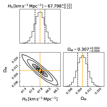
(b) Estimations for $\big{\{}H_{0},\Omega_{\rm M}\big{\}}$

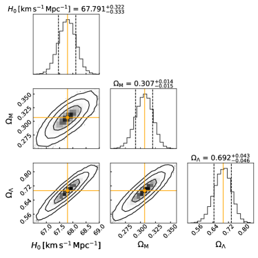
(c) Estimations for $\big{\{}H_{0},\Omega_{\rm M},\Omega_{\Lambda}\big{\}}$

Figure 8: Parameter estimations with DECIGO by using a realistic simulated galaxy catalog from the TAO.

4 Conclusion and discussion

Up to now, most of the detected GW events belong to the dark sirens in the context of cosmology. In the future, space-borne decihertz GW detectors can provide excellent localization capability for numerous detectable merger events. Therefore, it is possible to use these events to constrain cosmological parameters precisely by a statistic method. In this work, we explore how well the space-borne decihertz GW detectors (DO-Optimal and DECIGO) can constrain the cosmological parameters with simulated dark-siren events and galaxy catalogs. We have considered various redshift and luminosity distance errors and performed parameter estimations with single/multiple parameters for DO-Optimal and DECIGO. All the results are listed in Table 1, and we find that both DECIGO and DO-Optimal can constrain $H_{0}$ well. For 2-parameter/3-parameter estimations, DECIGO can still constrain $\Omega_{\rm M}$ and $\Omega_{\Lambda}$ well, while DO-Optimal cannot. The main reason is in DECIGO’s better localization accuracy compared with DO-Optimal. More recently, Seymour et al. [60] has shown that a space-borne decihertz detector can enhance the sensitivity of a ground network by about a factor of 3 for the cosmological parameter estimations with dark sirens. The precise measurements of $H_{0}$ with space-borne decihertz GW detectors can shed light on the $H_{0}$ tension. Early measurements constrained the relative error of $H_{0}$ to be larger than a few percents, while space-borne decihertz GW detectors can reach a better level. With the help of these detectors, we can use GW as another means to measure $H_{0}$ precisely and help us judge whether the two sets of results in the previous work for $H_{0}$ are valid.

Note that for realistic cosmological parameter estimations, galaxy catalogs would be incomplete due to the EM selection effects like the Malmquist bias [61]. Thus, in our work, we discuss the effect of Malmquist bias on the constraints of the cosmological parameters using DECIGO. We find that even taking into account the Malmquist bias, there are also many best-localized GW events and high-accuracy constraints on cosmological parameters. Moreover, several works have derived a correction term into the Bayesian framework to eliminate such a selection bias [18, 23, 62, 63]. Therefore, our results in this paper can still be used to provide meaningful references and helpful inputs for upcoming space-borne decihertz GW projects. In addition, the incompleteness of the galaxy catalog can be compensated by the GW-triggered deeper field galaxy surveys [64, 65, 66]. Moreover, one of the solutions to the lack of redshift information is to increase the EM follow-up observation. Several works have been devoted to the best searching strategy with ground-based GW observatories [67, 68, 69, 70] and the early warnings of EM follow-up observations from decihertz GW observatories [71, 72]. We will investigate these effects in the future. Finally, we have only considered circular orbits for SBBHs. Since the eccentricity can provide more astrophysical information [51, 73, 74, 75, 76], it is worth investigating whether the SBBH system with eccentricity will impact the estimation of the cosmological parameters [24].

References

- Abbott et al. [2016] B. P. Abbott et al. (LIGO Scientific, Virgo), Phys. Rev. Lett. 116, 061102 (2016), arXiv:1602.03837 [gr-qc] .
- Abbott et al. [2017a] B. P. Abbott et al. (LIGO Scientific, Virgo), Phys. Rev. Lett. 119, 161101 (2017a), arXiv:1710.05832 [gr-qc] .
- Abbott et al. [2021a] R. Abbott et al. (LIGO Scientific, Virgo), Phys. Rev. X 11, 021053 (2021a), arXiv:2010.14527 [gr-qc] .
- Abbott et al. [2021b] R. Abbott et al. (LIGO Scientific, VIRGO, KAGRA), (2021b), arXiv:2111.03604 [astro-ph.CO] .
- Schutz [1986] B. F. Schutz, Nature 323, 310 (1986).
- Dalal et al. [2006] N. Dalal, D. E. Holz, S. A. Hughes, and B. Jain, Phys. Rev. D 74, 063006 (2006), arXiv:astro-ph/0601275 .
- Holz and Hughes [2005] D. E. Holz and S. A. Hughes, Astrophys. J. 629, 15 (2005), arXiv:astro-ph/0504616 .
- Nissanke et al. [2010] S. Nissanke, D. E. Holz, S. A. Hughes, N. Dalal, and J. L. Sievers, Astrophys. J. 725, 496 (2010), arXiv:0904.1017 [astro-ph.CO] .
- Nissanke et al. [2013] S. Nissanke, D. E. Holz, N. Dalal, S. A. Hughes, J. L. Sievers, and C. M. Hirata, (2013), arXiv:1307.2638 [astro-ph.CO] .
- Abbott et al. [2021c] R. Abbott et al. (LIGO Scientific, VIRGO, KAGRA), (2021c), arXiv:2111.03634 [astro-ph.HE] .
- Abbott et al. [2017b] B. P. Abbott et al. (LIGO Scientific, Virgo, Fermi-GBM, INTEGRAL), Astrophys. J. Lett. 848, L13 (2017b), arXiv:1710.05834 [astro-ph.HE] .
- Abbott et al. [2017c] B. P. Abbott et al. (LIGO Scientific, Virgo, Fermi GBM, INTEGRAL, IceCube, AstroSat Cadmium Zinc Telluride Imager Team, IPN, Insight-Hxmt, ANTARES, Swift, AGILE Team, 1M2H Team, Dark Energy Camera GW-EM, DES, DLT40, GRAWITA, Fermi-LAT, ATCA, ASKAP, Las Cumbres Observatory Group, OzGrav, DWF (Deeper Wider Faster Program), AST3, CAASTRO, VINROUGE, MASTER, J-GEM, GROWTH, JAGWAR, CaltechNRAO, TTU-NRAO, NuSTAR, Pan-STARRS, MAXI Team, TZAC Consortium, KU, Nordic Optical Telescope, ePESSTO, GROND, Texas Tech University, SALT Group, TOROS, BOOTES, MWA, CALET, IKI-GW Follow-up, H.E.S.S., LOFAR, LWA, HAWC, Pierre Auger, ALMA, Euro VLBI Team, Pi of Sky, Chandra Team at McGill University, DFN, ATLAS Telescopes, High Time Resolution Universe Survey, RIMAS, RATIR, SKA South Africa/MeerKAT), Astrophys. J. Lett. 848, L12 (2017c), arXiv:1710.05833 [astro-ph.HE] .
- Coulter et al. [2017] D. A. Coulter et al., Science 358, 1556 (2017), arXiv:1710.05452 [astro-ph.HE] .
- Soares-Santos et al. [2017] M. Soares-Santos et al. (DES, Dark Energy Camera GW-EM), Astrophys. J. Lett. 848, L16 (2017), arXiv:1710.05459 [astro-ph.HE] .
- Cowperthwaite et al. [2017] P. S. Cowperthwaite et al., Astrophys. J. Lett. 848, L17 (2017), arXiv:1710.05840 [astro-ph.HE] .
- Goldstein et al. [2017] A. Goldstein et al., Astrophys. J. Lett. 848, L14 (2017), arXiv:1710.05446 [astro-ph.HE] .
- Savchenko et al. [2017] V. Savchenko et al., Astrophys. J. Lett. 848, L15 (2017), arXiv:1710.05449 [astro-ph.HE] .
- Abbott et al. [2017d] B. P. Abbott et al. (LIGO Scientific, Virgo, 1M2H, Dark Energy Camera GW-E, DES, DLT40, Las Cumbres Observatory, VINROUGE, MASTER), Nature 551, 85 (2017d), arXiv:1710.05835 [astro-ph.CO] .
- Fishbach et al. [2019] M. Fishbach et al. (LIGO Scientific, Virgo), Astrophys. J. Lett. 871, L13 (2019), arXiv:1807.05667 [astro-ph.CO] .
- Abbott et al. [2021d] B. P. Abbott et al. (LIGO Scientific, Virgo, VIRGO), Astrophys. J. 909, 218 (2021d), [Erratum: Astrophys.J. 923, 279 (2021)], arXiv:1908.06060 [astro-ph.CO] .
- Gray et al. [2020] R. Gray et al., Phys. Rev. D 101, 122001 (2020), arXiv:1908.06050 [gr-qc] .
- Zhao et al. [2020] Z.-W. Zhao, L.-F. Wang, J.-F. Zhang, and X. Zhang, Sci. Bull. 65, 1340 (2020), arXiv:1912.11629 [astro-ph.CO] .
- Zhu et al. [2022a] L.-G. Zhu, Y.-M. Hu, H.-T. Wang, J.-D. Zhang, X.-D. Li, M. Hendry, and J. Mei, Phys. Rev. Res. 4, 013247 (2022a), arXiv:2104.11956 [astro-ph.CO] .
- Zhu et al. [2022b] L.-G. Zhu, L.-H. Xie, Y.-M. Hu, S. Liu, E.-K. Li, N. R. Napolitano, B.-T. Tang, J.-d. Zhang, and J. Mei, Sci. China Phys. Mech. Astron. 65, 259811 (2022b), arXiv:2110.05224 [astro-ph.CO] .
- Liu et al. [2020a] C. Liu, L. Shao, J. Zhao, and Y. Gao, Mon. Not. Roy. Astron. Soc. 496, 182 (2020a), arXiv:2004.12096 [astro-ph.HE] .
- Isoyama et al. [2018] S. Isoyama, H. Nakano, and T. Nakamura, PTEP 2018, 073E01 (2018), arXiv:1802.06977 [gr-qc] .
- Riess et al. [2019] A. G. Riess, S. Casertano, W. Yuan, L. M. Macri, and D. Scolnic, Astrophys. J. 876, 85 (2019), arXiv:1903.07603 [astro-ph.CO] .
- Riess et al. [2021] A. G. Riess, S. Casertano, W. Yuan, J. B. Bowers, L. Macri, J. C. Zinn, and D. Scolnic, Astrophys. J. Lett. 908, L6 (2021), arXiv:2012.08534 [astro-ph.CO] .
- Aghanim et al. [2020] N. Aghanim et al. (Planck), Astron. Astrophys. 641, A6 (2020), [Erratum: Astron.Astrophys. 652, C4 (2021)], arXiv:1807.06209 [astro-ph.CO] .
- Kawamura et al. [2021] S. Kawamura et al., PTEP 2021, 05A105 (2021), arXiv:2006.13545 [gr-qc] .
- Amaro-Seoane et al. [2017] P. Amaro-Seoane, H. Audley, S. Babak, J. Baker, E. Barausse, P. Bender, E. Berti, P. Binetruy, M. Born, D. Bortoluzzi, et al., arXiv preprint arXiv:1702.00786 (2017).
- Sedda et al. [2020] M. A. Sedda et al., Class. Quant. Grav. 37, 215011 (2020), arXiv:1908.11375 [gr-qc] .
- Sedda et al. [2021] M. A. Sedda et al., Exper. Astron. 51, 1427 (2021), arXiv:2104.14583 [gr-qc] .
- Chen et al. [2022] J. Chen, C. Yan, Y. Lu, Y. Zhao, and J. Ge, Res. Astron. Astrophys. 22, 015020 (2022), arXiv:2201.12526 [astro-ph.CO] .
- Gordon et al. [2007] C. Gordon, K. Land, and A. Slosar, Phys. Rev. Lett. 99, 081301 (2007), arXiv:0705.1718 [astro-ph] .
- Kocsis et al. [2006] B. Kocsis, Z. Frei, Z. Haiman, and K. Menou, Astrophys. J. 637, 27 (2006), arXiv:astro-ph/0505394 .
- He [2019] J.-h. He, Phys. Rev. D 100, 023527 (2019), arXiv:1903.11254 [astro-ph.CO] .
- Ilbert et al. [2013] O. Ilbert et al., Astron. Astrophys. 556, A55 (2013), arXiv:1301.3157 [astro-ph.CO] .
- Hirata et al. [2010] C. M. Hirata, D. E. Holz, and C. Cutler, Phys. Rev. D 81, 124046 (2010), arXiv:1004.3988 [astro-ph.CO] .
- Graham et al. [2020] M. J. Graham et al., Phys. Rev. Lett. 124, 251102 (2020), arXiv:2006.14122 [astro-ph.HE] .
- Abbott et al. [2019] B. P. Abbott et al. (LIGO Scientific, Virgo), Astrophys. J. Lett. 882, L24 (2019), arXiv:1811.12940 [astro-ph.HE] .
- Ade et al. [2016] P. A. R. Ade et al. (Planck), Astron. Astrophys. 594, A13 (2016), arXiv:1502.01589 [astro-ph.CO] .
- Khan et al. [2016] S. Khan, S. Husa, M. Hannam, F. Ohme, M. Pürrer, X. J. Forteza, and A. Bohé, Phys. Rev. D 93, 044007 (2016).
- Husa et al. [2016] S. Husa, S. Khan, M. Hannam, M. Pürrer, F. Ohme, X. J. Forteza, and A. Bohé, Phys. Rev. D 93, 044006 (2016).
- Abadie et al. [2010] J. Abadie et al. (LIGO Scientific, VIRGO), Class. Quant. Grav. 27, 173001 (2010), arXiv:1003.2480 [astro-ph.HE] .
- Chen and Holz [2016] H.-Y. Chen and D. E. Holz, (2016), arXiv:1612.01471 [astro-ph.HE] .
- Soares-Santos et al. [2019] M. Soares-Santos et al. (DES, LIGO Scientific, Virgo), Astrophys. J. Lett. 876, L7 (2019), arXiv:1901.01540 [astro-ph.CO] .
- Palmese et al. [2020] A. Palmese et al. (DES), Astrophys. J. Lett. 900, L33 (2020), arXiv:2006.14961 [astro-ph.CO] .
- Nair et al. [2018] R. Nair, S. Bose, and T. D. Saini, Phys. Rev. D 98, 023502 (2018), arXiv:1804.06085 [astro-ph.CO] .
- Kelvin et al. [2014] L. S. Kelvin et al., Mon. Not. Roy. Astron. Soc. 444, 1647 (2014).
- Chen and Amaro-Seoane [2017] X. Chen and P. Amaro-Seoane, Astrophys. J. Lett. 842, L2 (2017), arXiv:1702.08479 [astro-ph.HE] .
- Finn [1992] L. S. Finn, Phys. Rev. D 46, 5236 (1992), arXiv:gr-qc/9209010 .
- Foreman-Mackey et al. [2013] D. Foreman-Mackey, D. W. Hogg, D. Lang, and J. Goodman, Publications of the Astronomical Society of the Pacific 125, 306 (2013).
- Foreman-Mackey et al. [2019] D. Foreman-Mackey, W. Farr, M. Sinha, A. Archibald, D. Hogg, J. Sanders, J. Zuntz, P. Williams, A. Nelson, M. de Val-Borro, T. Erhardt, I. Pashchenko, and O. Pla, Journal of Open Source Software 4, 1864 (2019).
- Klypin et al. [2016] A. Klypin, G. Yepes, S. Gottlöber, F. Prada, and S. Heß, Mon. Not. Roy. Astron. Soc. 457, 4340 (2016).
- Croton et al. [2016] D. J. Croton, A. R. H. Stevens, C. Tonini, T. Garel, M. Bernyk, A. Bibiano, L. Hodkinson, S. J. Mutch, G. B. Poole, and G. M. Shattow, Astrophys. J. Suppl. 222, 22 (2016), arXiv:1601.04709 [astro-ph.GA] .
- Conroy and Wechsler [2009] C. Conroy and R. H. Wechsler, Astrophys. J. 696, 620 (2009), arXiv:0805.3346 [astro-ph] .
- York et al. [2000] D. G. York et al. (SDSS), Astron. J. 120, 1579 (2000), arXiv:astro-ph/0006396 .
- Laureijs et al. [2011] R. Laureijs et al. (EUCLID), (2011), arXiv:1110.3193 [astro-ph.CO] .
- Seymour et al. [2022] B. C. Seymour, H. Yu, and Y. Chen, (2022), arXiv:2208.01668 [gr-qc] .
- Malmquist [1922] K. G. Malmquist, Meddelanden fran Lunds Astronomiska Observatorium Serie I 100, 1 (1922).
- Chen et al. [2018] H.-Y. Chen, M. Fishbach, and D. E. Holz, Nature 562, 545 (2018), arXiv:1712.06531 [astro-ph.CO] .
- Mandel et al. [2019] I. Mandel, W. M. Farr, and J. R. Gair, Mon. Not. Roy. Astron. Soc. 486, 1086 (2019), arXiv:1809.02063 [physics.data-an] .
- Bartos et al. [2015] I. Bartos, A. P. S. Crotts, and S. Márka, Astrophys. J. Lett. 801, L1 (2015), arXiv:1410.0677 [astro-ph.HE] .
- Chen and Holz [2017] H.-Y. Chen and D. E. Holz, Astrophys. J. 840, 88 (2017), arXiv:1509.00055 [astro-ph.IM] .
- Klingler et al. [2019] N. J. Klingler et al., Astrophys. J. Suppl. 245, 15 (2019), arXiv:1909.11586 [astro-ph.HE] .
- Gehrels et al. [2016] N. Gehrels, J. K. Cannizzo, J. Kanner, M. M. Kasliwal, S. Nissanke, and L. P. Singer, Astrophys. J. 820, 136 (2016), arXiv:1508.03608 [astro-ph.HE] .
- Rosswog et al. [2017] S. Rosswog, U. Feindt, O. Korobkin, M. R. Wu, J. Sollerman, A. Goobar, and G. Martinez-Pinedo, Class. Quant. Grav. 34, 104001 (2017), arXiv:1611.09822 [astro-ph.HE] .
- Cowperthwaite et al. [2019] P. S. Cowperthwaite, V. A. Villar, D. M. Scolnic, and E. Berger, Astrophys. J. 874, 88 (2019), arXiv:1811.03098 [astro-ph.HE] .
- Liu et al. [2022a] M.-X. Liu, H. Tong, Y.-M. Hu, M. L. Chan, Z. Liu, H. Sun, and M. Hendry, Res. Astron. Astrophys. 21, 308 (2022a), arXiv:2005.11076 [astro-ph.HE] .
- Kang et al. [2022] Y. Kang, C. Liu, and L. Shao, Mon. Not. Roy. Astron. Soc. 515, 739 (2022), arXiv:2205.02104 [astro-ph.HE] .
- Liu et al. [2022b] C. Liu, Y. Kang, and L. Shao, Astrophys. J. 934, 84 (2022b), arXiv:2204.06161 [astro-ph.HE] .
- Liu et al. [2020b] X. Liu, Z. Cao, and L. Shao, Phys. Rev. D 101, 044049 (2020b), arXiv:1910.00784 [gr-qc] .
- Gerosa et al. [2019] D. Gerosa, S. Ma, K. W. K. Wong, E. Berti, R. O’Shaughnessy, Y. Chen, and K. Belczynski, Phys. Rev. D 99, 103004 (2019), arXiv:1902.00021 [astro-ph.HE] .
- Zhang et al. [2019] F. Zhang, L. Shao, and W. Zhu, Astrophys. J. 877, 87 (2019), arXiv:1903.02685 [astro-ph.GA] .
- Nishizawa et al. [2016] A. Nishizawa, E. Berti, A. Klein, and A. Sesana, Phys. Rev. D 94, 064020 (2016), arXiv:1605.01341 [gr-qc] .