Magnetization Plateau of the Distorted Diamond Spin Chain with Anisotropic Ferromagnetic Interaction

Abstract

The $S=1/2$ distorted diamond spin chain with the anisotropic ferromagnetic interaction is investigated using the numerical diagonalization and the level spectroscopy analysis. It is known that the system exhibits a plateau of the magnetization curve at the 1/3 of the saturation. The present study indicates that as the anisotropy is varied the quantum phase transition occurs between two different mechanisms of the 1/3 magnetization plateau. The phase diagram with respect to the anisotropy and the ferromagnetic coupling is also presented.

I Introduction

The magnetization plateau is one of interesting phenomena in the field of the magnetism. It possibly appears as the quantization of magnetization, when the one-dimensional quantum spin system satisfies the necessary condition

$$S_{\rm unit}-m_{\rm unit}={\rm integer},$$ (1)

where $S_{\rm unit}$ is the total spin and $m_{\rm unit}$ is the magnetization per unit celloshikawa . The $S=1/2$ distorted diamond spin chainokamoto0 is a strongly frustrated quantum spin system which exhibits the 1/3 magnetization plateau according to the conditions. This system was proposed as a good theoretical model of the compound Cu₃(CO₃)₂(OH)₂, called azuritekikuchi ; kikuchi2 . In fact, the magnetization measurement of azurite detected a clear magnetization plateau at 1/3 of the saturation magnetization. The theoretical study by the numerical exact diagonalizationokamoto1 ; okamoto2 suggested that the 1/3 magnetization plateau is induced by two different mechanisms. One is based on the ferrimagnetic mechanism and the other is due to the formation of singlet dimers at the $J_{2}$ bonds in Fig.1 and free spins. The 1/3 plateau of azurite is believed to be due to the latter mechanism kikuchi2 ; aimo

Recently other candidate materials for the distorted diamond spin chain were discovered. They are the compound K₃Cu₃AlO₂(SO₄)₄, called alumoklyuchevskitefujihara ; morita ; fujihala2 and related materials. All the exchange interactions of azurite are antiferromagnet, while alumoklyuchevskite includes ferromagnetic couplings as well as antiferromagnetic ones. The most important point is the the difference of the $J_{2}$ bond, although the model of alumoklyuchevskite is more complicated than that of azurite. The $J_{2}$ bond is antiferromagnetic on which a singlet dimer pair is formed in azurite, whereas it is ferromagnetic in alumoklyuchevskite. Thus it would be useful to investigate the distorted diamond chain with the ferromagnetic interaction. In this paper we investigate the distorted diamond spin chain model with the ferromagnetic exchange interaction and introduce the $XXZ$ anisotropy to this ferromagnetic bond. It is expected that this model would exhibit the 1/3 magnetization plateau based on two different mechanisms, as was predicted for the $(S,s)=(1,1/2)$ mixed spin chainsakai-okamoto . Using the numerical diagonalization of finite-size systems and the level spectroscopy analysis, we investigate the mechanisms of the 1/3 magnetization plateau in the present model and obtain the phase diagram with respect to the anisotropy and the strength of the ferromagnetic coupling.

II Model

We investigate the model described by the Hamiltonian

$${\cal H} = {\cal H}_{0}+{\cal H}_{\rm Z}$$ (2)

$${\cal H}_{0} = J_{1}\sum_{j=1}^{N/3}\left[{\bf S}_{3j-2}\cdot{\bf S}_{3j-1}+{\bf S}_{3j-1}\cdot{\bf S}_{3j}\right]$$

$$+J_{2}\sum_{j=1}^{N/3}\left[S_{3j}^{x}S_{3j+1}^{x}+S_{3j}^{y}S_{3j+1}^{y}+\lambda S_{3j}^{z}S_{3j+1}^{z}\right]$$

$$+J_{3}\sum_{j=1}^{N/3}\left[{\bf S}_{3j-1}\cdot{\bf S}_{3j+1}+{\bf S}_{3j}\cdot{\bf S}_{3j+2}\right]$$ (3)

$${\cal H}_{\rm Z} = -H\sum_{l=1}^{N}S_{l}^{z}$$ (4)

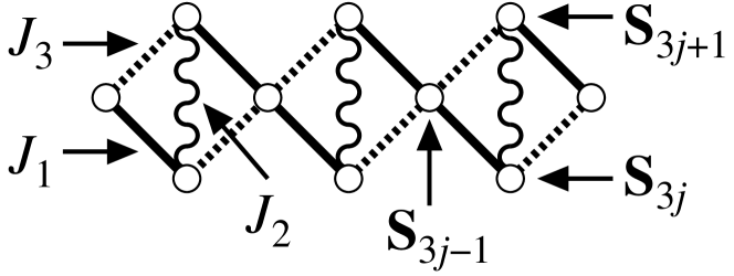
Figure 1: The model of the $S=1/2$ distorted diamond spin chain. Solid lines, wavy lines and dotted lines denote $J_{1}$, $J_{2}$ and $J_{3}$, respectively.

where ${\bf S}_{j}$ is the spin-1/2 operator, $J_{1}$, $J_{2}$, $J_{3}$ are the coupling constants of the exchange interactions, respectively, and $\lambda$ is the coupling anisotropy. The schematic picture of the model is shown in Fig. 1. In this paper we consider the case where $J_{2}$ is ferromagnetic and the $XY$-like (easy-plane) anisotropy is introduced to this bond only ($J_{2}<0$ and $\lambda<1$), while $J_{1}$ and $J_{3}$ are isotropic antiferromagnetic bonds ($J_{1},J_{3}>0$ ). (We note that the case of $J_{1}<0$, $J_{2}>0$, $J_{3}\gtrless 0$ and $\lambda=1$ was studied. okamoto2005 ). $N$ is the number of spins and $L$ is defined as the number of the unit cells, namely $N=3L$. For $L$-unit systems, the lowest energy of ${\cal H}_{0}$ in the subspace where $\sum_{j}S_{j}^{z}=M$, is denoted as $E(L,M)$. The reduced magnetization $m$ is defined as $m=M/M_{\rm s}$, where $M_{\rm s}$ denotes the saturation of the magnetization, namely $M_{\rm s}=3L/2$ for this system. $E(L,M)$ is calculated by the Lanczos algorithm under the periodic boundary condition (${\bf S}_{N+l}={\bf S}_{l}$) and the twisted boundary condition ($S^{x,y}_{N+l}=-S^{x.y}_{l},S^{z}_{N+l}=S^{z}_{l}$), for $L=$4, 6 and 8. Under the twisted boundary condition we calculate the lowest energy $E_{{\rm TBC},P=+}(L,M)$ ($E_{{\rm TBC},P=-}(L,M)$) in the subspace where the parity is even (odd) with respect to the lattice inversion ${\bf S}_{l}\to{\bf S}_{N-l+1}$ at the twisted bond.

III Magnetization plateau

In the isotropic coupling case $\lambda=1$ the model (2) is the ferrimagnet with the 1/3 spontaneous magnetization and has the 1/3 magnetization plateau. The previous numerical diagonalization and the level spectroscopy studysakai-okamoto on the $(S,s)=(1,1/2)$ mixed spin ferrimagnetic chain indicated that as the easy-plane anisotropy increases, the system exhibits the quantum phase transition at the critical point where the ferrimagnetic magnetization plateau disappears and a new plateau due to another mechanism appears. The equivalent quantum phase transition is expected to occur in the present model. The initial 1/3 magnetization plateau is based on the ferrimagnetic mechanism shown in Fig. 2, while another mechanism of the 1/3 plateau is expected to be due to a strong easy-plane anisotropy effect shown in Fig. 3. We denote these two plateaux as the plateaux I and II, respectively.

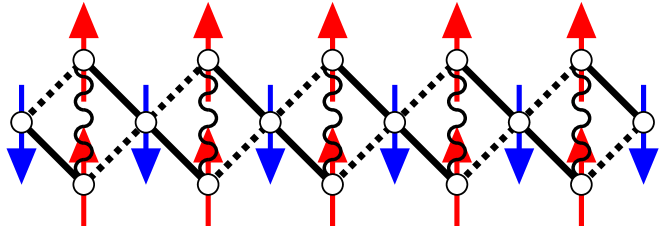
Figure 2: Schematic picture of the ferrimagnetic mechanism of the 1/3 magnetization plateau.

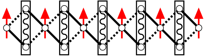
Figure 3: Schematic picture of another mechanism of the 1/3 magnetization plateau, induced by the strong easy-plane anisotropy of the ferromagnetic $J_{2}$ bond. Here the rectangles denote the two spin state $(1/\sqrt{2})(\uparrow\downarrow+\downarrow\uparrow)$.

In order to investigate the quantum phase transition between the plateaux I and II, we apply the phenomenological renormalization for the plateau width $W=E(L,M+1)+E(L,M-1)-2E(L,M)$ at $M=L/2$ calculated by the numerical diagonalization. The scaled plateau width $LW$ for $L=$4, 6 and 8 is plotted versus the anisotropy $\lambda$ in the case of $J_{1}=1.0,J_{2}=-1.0$ and $J_{3}=0.5$ shown in Fig. 4. It indicates the quantum phase transition around $\lambda\sim 0.2$ where the first plateau vanishes and the other plateau appears with decreasing $\lambda$. The phase boundary will be estimated in the next section.

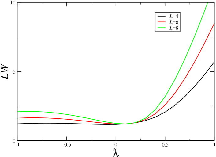
Figure 4: Scaled plateau width $LW$ for $L=$4, 6 and 8 is plotted versus the anisotropy $\lambda$ in the case of $J_{1}=1.0,J_{2}=-1.0$ and $J_{3}=0.5$

IV Level spectroscopy and phase diagram

In order to detect the quantum phase transitions among the plateaux I, II and plateauless phases, the level spectroscopy analysiskitazawa1 ; kitazawa2 is one of the best methods. According to this analysis, we should compare the following three energy gaps;

$$\Delta_{2}={E(L,M-2)+E(L,M+2)-2E(L,M)\over 2},$$ (5)

$$\Delta_{{\rm TBC},P=+}=E_{{\rm TBC},P=+}(L,M)-E(L,M),$$ (6)

$$\Delta_{{\rm TBC},P=-}=E_{{\rm TBC},P=-}(L,M)-E(L,M).$$ (7)

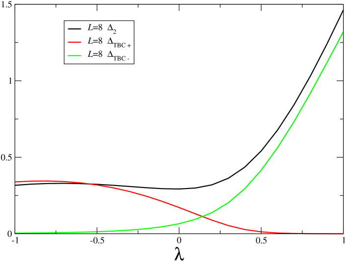
Figure 5: Level spectroscopy analysis applied to the present model for $J_{1}=1.0$, $J_{2}=-1.0$ and $J_{3}=0.5$.

The level spectroscopy method indicates that the smallest gap among these three gaps for $M=L=M_{\rm s}/3$ determines the phase at $m=1/3$. $\Delta_{2}$, $\Delta_{{\rm TBC},P=+}$ and $\Delta_{{\rm TBC},P=-}$ correspond to the plateauless, plateau I and plateau II phases, respectively. Especially, $\Delta_{{\rm TBC,}P=+}$ and $\Delta_{{\rm TBC},P=-}$ directly reflect the symmetries of two plateau states. The physical explanation is very simple. In the ferrimagnetic mechanism, the state is essentially composed of the direct product of local state, which leads to no change ($P=+$) under the space inversion operation. On the other hand, there is a two-spin state $(1/\sqrt{2})(\uparrow_{N}\downarrow_{1}+\downarrow_{1}\uparrow_{N})$ on the $J_{2}$ bonds connecting ${\bf S}_{N}$ and ${\bf S}_{1}$. This state changes into the $(1/\sqrt{2})(\uparrow_{N}\downarrow_{1}-\downarrow_{1}\uparrow_{N})$ state if the corresponding $J_{2}$ bond is twisted. When we perform the space inversion operation, this state becomes $(1/\sqrt{2})(\downarrow_{1}\uparrow_{N}-\uparrow_{1}\downarrow_{N})$, which means $P=-$. The $\lambda$ dependence of these three gaps for $J_{1}=1.0$, $J_{2}=-1.0$ and $J_{3}=0.5$ is shown in Fig. 5 for $L=$8. It indicates that the quantum phase transition between the plateaux I and II phases occurs, but the plateauless phase does not appear.

Assuming that the finite-size correction is proportional to $1/L^{2}$, we estimate the phase boundaries in the thermodynamic limit from every level-cross point. The process for the same parameters as Fig. 5 is shown in Fig. 6.

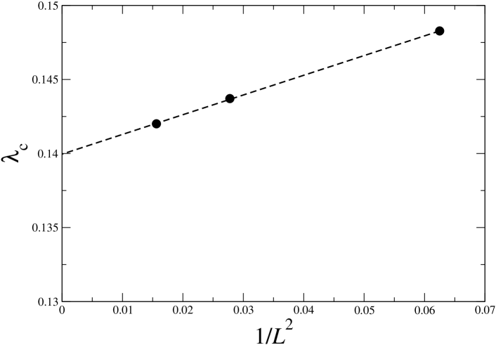
Figure 6: Process of the extrapolation of the phase boundary to the thermodynamic limit $L\rightarrow\infty$. The model parameters are the same as those of Fig.5.

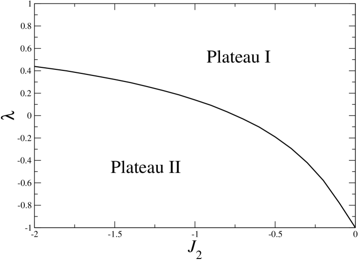
Figure 7: Phase diagram on the $J_{2}$-$\lambda$ plane at $m=1/3$ for $J_{1}=1.0$ and $J_{3}=0.5$.

The phase diagram on the $J_{2}$-$\lambda$ plane at $m=1/3$ for $J_{1}=1.0$ and $J_{3}=0.5$ is shown in Fig. 7. The two different plateau phases appears, but the plateauless phase does not appear. The plateau II phase is predicted for the first time at least for the distorted diamond spin system.

V Summary

The $S=1/2$ distorted diamond spin chain with the anisotropic ferromagnetic interaction is investigated using the numerical diagonalization and the level spectroscopy analysis. As a result it is found that as the easy-plane anisotropy of the ferromagnetic bond increases the quantum phase transition occurs at the critical point where the mechanism of the 1/3 magnetization plateau changes. The phase diagram with respect to the strength of the ferromagnetic coupling and the anisotropy is also presented.

Data Availability

The data that support the findings of this study are available from the corresponding author upon reasonable request.

References

- (1) M. Oshikawa, M. Yamanaka and I. Affleck, Phys. Rev. Lett. 78, 1984 (1997).
- (2) K. Okamoto T. Tonegawa, Y. Takahashi, and M. Kaburagi, J. Phys.: Condens. Matter 11, 10485 (1999).
- (3) H. Kikuchi, Y. Fujii, M. Chiba, S. Mitsudo, T. Idehara, T. Tonegawa, K. Okamoto, T. Sakai, T. Kuwai, and H. Ohta, Phys. Rev. Lett. 94, 227201 (2005).
- (4) H. Kikuchi, Y. Fujii, M. Chiba, S. Mitsudo, T. Idehara, T. Tonegawa, K. Okamoto, T. Sakai, T. Kuwai, K. Kindo, A. Matsuo, W. Higemoto, K. Nishiyama, M. Holvatoć and C. Bertheir, Prog. Theor. Phys. Suppl. No.159, 1 (2005).
- (5) F. Aimo, S. Krämer, M. Klanjšek, M. Horvatić, C. Berthier, and H. Kikuchi, Phys. REv. Lett. 102, 127205 (2009).
- (6) K. Okamoto, T. Tonegawa, and M. Kaburagi, J. Phys.: Condens. Matter, 15, 5979 (2003).
- (7) K. Okamoto and A. Kitazawa, J. Phys. A: Math. Gen. 32, 4601 (1999).
- (8) M. Fujihala, H. Koorikawa, S. Mitsuda, M. Hagihala, H. Morodomi, T. Kawae, A. Mitsudo, and K. Kindo, J. Phys. Soc. Jpn. 84, 073702 (2015).
- (9) K. Morita, M. Fujihala, H. Koorikawa, T. Sugimoto, S. Sota, S. Mitsuda and T. Tohyama, Phys. Rev. B 95, 184412 (2017).
- (10) M. Fujihala, H. Koorikawa1, S. Mitsuda, K. Morita, T. Tohyama, K. Tomiyasu, A. Koda, H. Okabe, S. Itoh, T. Yokoo, S. Ibuka, M. Tadokoro, M. Itoh, H. Sagayama, R. Kumai and Y. Murakami, Sci. Rep. 7, 16785 (2017)
- (11) K. Okamoto, T. Tonegawa, T. Yamada, M. Matsumoto, M. Koga and T. Sakai, Prog. Theor. Phys. Suppl. No.159, 17 (2005).
- (12) T. Sakai and K. Okamoto, Phys. Rev. B 65, 214403 (2002).
- (13) A. Kitazawa, J. Phys. A: Math. Gen. 30, L285 (1997).
- (14) K. Nomura and A. Kitazawa, J. Phys. A: Math. Gen. 31, 7341 (1998).