REMuS-GNN: A Rotation-Equivariant Model for Simulating Continuum Dynamics

Abstract

Numerical simulation is an essential tool in many areas of science and engineering, but its performance often limits application in practice or when used to explore large parameter spaces. On the other hand, surrogate deep learning models, while accelerating simulations, often exhibit poor accuracy and ability to generalise. In order to improve these two factors, we introduce REMuS-GNN, a rotation-equivariant multi-scale model for simulating continuum dynamical systems encompassing a range of length scales. REMuS-GNN is designed to predict an output vector field from an input vector field on a physical domain discretised into an unstructured set of nodes. Equivariance to rotations of the domain is a desirable inductive bias that allows the network to learn the underlying physics more efficiently, leading to improved accuracy and generalisation compared with similar architectures that lack such symmetry. We demonstrate and evaluate this method on the incompressible flow around elliptical cylinders.

1 Introduction

Continuum dynamics models often describe the underlying physical laws by one or more partial differential equations (PDEs). Numerical methods are well-established for approximately solving PDEs with high accuracy, however, they are computationally expensive (Karniadakis & Sherwin, 2013). Deep learning techniques have been shown to accelerate physical simulations (Guo et al., 2016), however, their relatively poor accuracy and limited ability to generalise restricts their application in practice. Most deep learning models for simulating continuum physics have been developed around convolutional neural networks (CNNs) (Thuerey et al., 2018; Wiewel et al., 2019). CNNs constrain input and output fields to be defined on rectangular domains represented by regular grids, which is not suitable for more complex domains. This has motivated the recent interest in graph neural networks (GNN) for learning to simulate continuum dynamics, which allow complex domains to be represented and the resolution spatially varied (Pfaff et al., 2021).

Most physical processes possess several symmetries, among which translation and rotation are perhaps the most common. Translation invariance/equivariance can be easily satisfied by using CNNs or GNNs (Battaglia et al., 2018). For rotation, the general approach is to approximately learn invariance/equivariance by training against augmented training data which includes rotations (Chu & Thuerey, 2017; Li et al., 2019; Mrowca et al., 2018; Lino et al., 2021). Here, we propose REMuS-GNN, a Rotation Equivariant Multi-Scale GNN model that enforces the rotation equivariance of input and output vector fields, and improves the accuracy and generalisation over the data-augmentation approach. REMuS-GNN forecasts the spatio-temporal evolution of continuum systems, discretised on unstructured sets of nodes, and processes the physical data at different resolutions or length scales, enabling the network to more accurately and efficiently learn spatially global dynamics. We introduce a general directional message-passing (MP) algorithm and an edge-unpooling algorithm that is rotation invariant. The accuracy and generalisation of REMuS-GNN was assessed on simulations of the incompressible flow around elliptical cylinders, an example of Eulerian dynamics with a global behaviour due the infinite speed of the pressure waves.

2 Related work

Neural solvers

During the last five years, most of the neural network models used for simulating continuum physics have included convolutional layers. For instance, CNNs have been used to solve the Poisson’s equation (Tang et al., 2018; Özbay et al., 2019) and to solve the Navier-Stokes equations (Guo et al., 2016; Thuerey et al., 2018; Lee & You, 2019; Kim et al., 2019; Wiewel et al., 2019), achieving an speed-up of one to four orders of magnitude with respect to numerical solvers. To the best of our knowledge Alet et al. (2019) were the first to explore the use of GNNs to infer continuum physics by solving the Poisson PDE, and subsequently Pfaff et al. (2021) proposed a mesh-based GNN to simulate a wide range of continuum dynamics. Multi-resolution graph models were later introduced by Li et al. (2020); Lino et al. (2021); Liu et al. (2021) and Chen et al. (2021).

Rotation invariance and equivariance

There has been a constant interest to develop neural networks that are equivariant to symmetries, and particularly to rotation. For instance, Weiler & Cesa (2019) and Weiler et al. (2018) introduced an SE(2)-equivariant and an SE(3)-equivariant CNNs respectively, both later applied to simulate continuum dynamics by Wang et al. (2021) and Siddani et al. (2021). However, rotation equivariant CNNs only achieve equivariance with respect to a small set of rotations, unlike rotation equivariant GNNs (Thomas et al., 2018; Fuchs et al., 2020; Schütt et al., 2021; Satorras et al., 2021). All these rotation equivariant networks require a careful design of each of their components. On the other hand, rotation invariant GNNs, such as directional MP neural networks (Klicpera et al., 2020; 2021b), ensure the rotation invariance by a proper selection of the input and output attributes (Klicpera et al., 2021a; Liu et al., 2022). Nevertheless, these GNNs can only be applied to scalar fields, but not vector fields (Klicpera et al., 2020). On the other hand, although Tensor Flow Networks (Thomas et al., 2018) and SE(3)-Transformers (Fuchs et al., 2020) can handle equivariant vector fields and could be applied to Eulerian dynamics, they lack an efficient mechanism for processing and propagating node features across long distances.

3 REMuS-GNN

For a PDE $\frac{\partial\bm{u}}{\partial t}=\mathcal{F}(\bm{u})$ on a spatial domain $\mathcal{D}\subset\mathbb{R}^{2}$, REMuS-GNN infers the temporal evolution of the two-dimensional vector field $\bm{u}(t,\bm{x})$ at a finite set of nodes $V^{1}$, with coordinates $\bm{x}^{1}_{i}\in\mathcal{D}$. Given an input vector field $\bm{u}(t_{0},\bm{x}_{V^{1}})$ at time $t=t_{0}$ and at the $V^{1}$ nodes, a single evaluation of REMuS-GNN returns the output field $\bm{u}(t_{0}+dt,\bm{x}_{V^{1}})$, where $dt$ is a fixed time-step size. REMuS-GNN is equivariant to rotations of $\mathcal{D}$, i.e., if a two-dimensional rotation $\mathcal{R}:\bm{x}\rightarrow R\bm{x}$ with $R\in\mathbb{R}^{2\times 2}$ is applied to $\bm{x}_{V^{1}}$ and $\bm{u}(t_{0},\bm{x}_{V^{1}})$ then the output field is $R\bm{u}(t_{0}+dt,\bm{x}_{V^{1}})$. Such rotation equivariance is achieved through the selection of input attributes that are agnostic to the orientation of the domain (but still contain information about the relative position of the nodes) and the design of a neural network that is invariant to rotations. REMuS-GNN is applied to a data structure expanded from a directed graph. We denote it as $H^{1}:=(V^{1},E^{1},A^{1})$, where $E^{1}:=\{(i,j)|i,j\in V^{1}\}$ is a set of directed edges and $A^{1}:=\{(i,j,k)|(i,j),(j,k)\in E^{1}\}$ is a set of directed angles. The edges in $E^{1}$ are obtained using a k-nearest neighbours (k-NN) algorithm that guarantees that each node has exactly $\kappa$ incoming edges. Unlike traditional GNNs, there are no input node-attributes to the network. The input attributes at edge $(i,j)$ are $\bm{e}_{ij}:=[u_{ij},p(\bm{x}_{j}),\Omega_{j}]$, where $p(\bm{x})$ can be any physical parameter and $\Omega_{j}=1$ on Dirichlet boundaries and $\Omega_{j}=0$ elsewhere. The edge attribute $u_{ij}$ is defined as

$$u_{ij}:=\hat{\bm{e}}_{ij}\cdot\bm{u}(t_{0},\bm{x}_{j}),$$ (1)

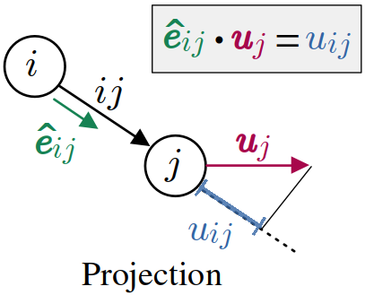
(a)

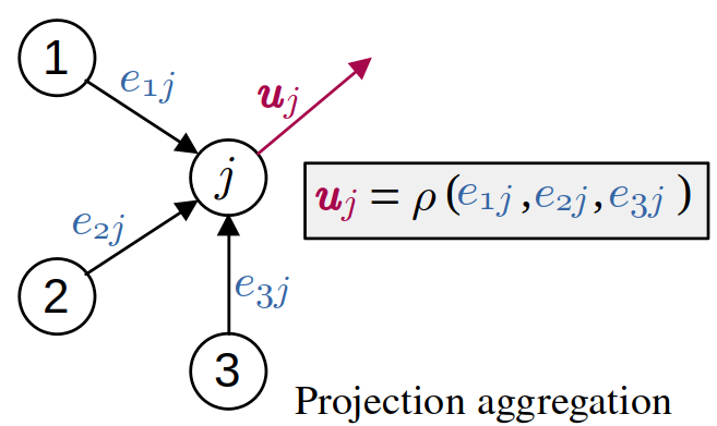
(b)

Figure 2: Diagrams of the projection step and projection-aggregation step (with $\kappa=3$). The projection allows to encode a vector defined at node $j$, $\bm{u}_{j}$, as its projection along the direction of the $\kappa$ incoming edges. The projection-aggregation is equivalent to the inverse of the projection step. Given the projection of $\bm{u}_{j}$ along the $\kappa$ incoming edges, $e_{1:\kappa,j}$; it restores the vector $\bm{u}_{j}$ by solving the overdetermined system of equations given by equation (2).

where $\hat{\bm{e}}_{ij}:=(\bm{x}_{j}-\bm{x}_{i})/||\bm{x}_{j}-\bm{x}_{i}||_{2}$; that is, $u_{ij}$ is the projection of the input vector field at node $j$ along the direction of the incoming edge $(i,j)$ (see Figure 2a). The input attributes at angle $(i,j,k)$ are $\bm{a}_{ijk}:=[||\bm{x}_{j}-\bm{x}_{i}||_{2},||\bm{x}_{k}-\bm{x}_{j}||_{2},\cos(\alpha_{ijk}),\sin(\alpha_{ijk})],$ where $\alpha_{ijk}:=\measuredangle(i,j)(j,k)$. Since all the input attributes are independent of the chosen coordinate system, any function applied exclusively to them is invariant to both rotations and translations.

We denote as $u^{\prime}_{ij}\in\mathbb{R}$ to the output at edge $(i,j)$ of a forward pass through the network, and it represents the projection of the output vector field at node $j$ along the direction of the incoming edge $(i,j)$. In order to obtain the desired output vectors at each node, $\bm{u}(t_{0}+dt,\bm{x}_{V^{1}})$, from these scalar values; we solve the overdetermined system of equations (if $\kappa>2$) given by

$$[\hat{\bm{e}}^{1}_{1:\kappa,j}][\bm{u}(t_{0}+dt,\bm{x}_{j})]=[u^{\prime}_{1:\kappa,j}],\ \ \ \forall j\in V^{1},$$ (2)

where matrix $[\hat{\bm{e}}_{1:\kappa,j}]\in\mathbb{R}^{\kappa\times 2}$ contains in its rows the unit vectors along the directions of the $\kappa$ incoming edges at node $j$, $[\bm{u}(t_{0}+dt,\bm{x}_{j})]\in\mathbb{R}^{2\times 1}$ is a column vector with the horizontal and vertical components of the output vector field at node $j$, and $[u^{\prime}_{1:\kappa,j}]\in\mathbb{R}^{\kappa\times 1}$ is another column vector with the value of $u^{\prime}$ at each of the $\kappa$ incoming edges. This step can be regarded as the inverse of the projection in equation (1). To solve equation (2) we use the Moore-Penrose pseudo-inverse of $[\hat{\bm{e}}_{1:\kappa,j}]$, which we denote as $[\hat{\bm{e}}_{1:\kappa,j}]^{+}\in\mathbb{R}^{2\times\kappa}$. Thus, if we define the projection-aggregation function at scale $\ell$, $\rho^{\ell}:\mathbb{R}^{\kappa}\rightarrow\mathbb{R}^{2}$, as the matrix-vector product given by

$$\rho^{\ell}(e_{1},e_{2},\dots,e_{\kappa}):=[\hat{\bm{e}}^{\ell}_{1:\kappa,j}]^{+}[e_{1},e_{2},\dots,e_{\kappa}]^{T}$$ (3)

then $\bm{u}(t_{0}+dt,\bm{x}_{j})=\rho^{1}(u^{\prime}_{1:\kappa,j})$ (see Figure 2b).

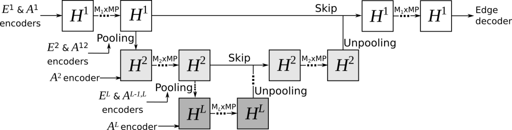
Figure 3: REMuS-GNN architecture. $H^{1}$ is a high-resolution representation, $H^{\ell}$ with $\ell\geq 2$ are lower-resolution representations.

The output $\bm{u}(t_{0}+dt,\bm{x}_{V^{1}})$ can be successively re-fed to REMuS-GNN to produce temporal roll-outs. In each forward pass the information processing happens at $L$ length-scales in a U-Net fashion, as illustrated in Figure 3. A single MP layer applied to $H^{1}$ propagates the edge features only locally between adjacent edges. To process the information at larger length-scales, REMuS-GNN creates an $H$ representation for each level, where MP is also applied. The lower-resolution representations ($H^{2},H^{3},\dots,H^{L}$; with $|V_{1}|>|V_{2}|>\dots>|V_{L}|$) possess fewer nodes, and hence, a single MP layer can propagate the features of edges and angles over longer distances more efficiently. Each $V^{\ell+1}$ is a subset of $V^{\ell}$ obtained using Guillard’s coarsening algorithm (Guillard, 1993), and $E^{\ell+1}$ and $A^{\ell+1}$ are obtained in an analogous manner to how $E^{1}$ and $A^{1}$ were obtained, as well as their attributes $\bm{e}_{ij}^{\ell+1}$ and $\bm{a}_{ij}^{\ell+1}$. Before being fed to the network, all the edge attributes $\bm{e}_{ij}^{\ell}$ and angle attributes $\bm{a}_{ij}^{\ell}$ are encoded through independent multi-layer perceptrons (MLPs). At the end, another MLP decodes the output edge-features of $E^{1}$ to return $u^{\prime}_{ij}$. As depicted in Figure 3, the building blocks of REMuS-GNN’s network are a directional MP (EdgeMP) layer, an edge-pooling layer and an edge-unpooling layer.

EdgeMP layer

Based on the GNBlock introduced by Sanchez-Gonzalez et al. (2018) and Battaglia et al. (2018) to update node and edge attributes, we define a general MP layer to update angle and edge attributes. The angle-update, angle-aggregation and edge-update at scale $\ell$ are given by

$$\bm{a}^{\ell}_{ijk} \leftarrow f^{a}([\bm{a}^{\ell}_{ijk},\bm{e}^{\ell}_{ij},\bm{e}^{\ell}_{jk}]),\ \ \ \forall(i,j,k)\in A^{\ell},$$ (4)

$$\overline{\bm{a}}^{\ell}_{jk} \leftarrow\frac{1}{\kappa}\sum_{k\in\mathcal{N}^{-}_{j}}\bm{a}^{\ell}_{ijk},\ \forall(j,k)\in E^{\ell},$$ (5)

$$\bm{e}^{\ell}_{jk} \leftarrow f^{e}([\bm{e}_{jk},\overline{\bm{a}}^{\ell}_{jk}]),\ \forall(j,k)\in E^{\ell}.$$ (6)

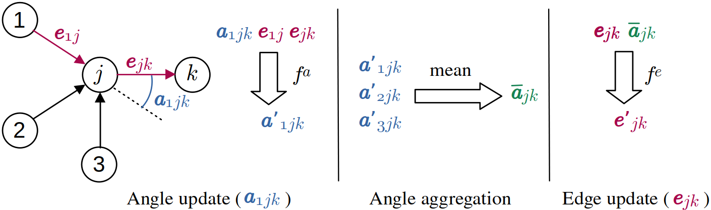
Figure 4: Diagram of the EdgeMP algorithm applied to update the edge attribute $\bm{e}_{jk}$ (in the diagram $\kappa=3$). The algorithm has three steps: update of the angle attributes, aggregation of the angle attributes and update of the edge attributes. In this case the angle-update step must be repeated 3 times (once for each incoming edge at node $j$).

Functions $f^{a}$ and $f^{e}$ are MLPs in the present work. This algorithm is illustrated in Figure 4.

Edge-pooling layer

Given a node $j\in V^{\ell}$ (hence $j\in V^{\ell-1}$ too), an outgoing edge $(j,k)\in E^{\ell}$ and its $\kappa$ incoming edges $(i,j)\in E^{\ell-1}$, we can define $\kappa$ new angles $(i,j,k)\in A^{\ell-1,\ell}$ that connect scale $\ell-1$ to scale $\ell$. Pooling from $H^{\ell-1}$ to $H^{\ell}$ is performed as the EdgeMP, but using the incoming edges $(i,j)\in E^{\ell-1}$, outcoming edge $(j,k)\in E^{\ell}$ and angles $(i,j,k)\in A^{\ell-1,\ell}$.

Edge-unpooling layer

To perform the unpooling from $H^{\ell+1}$ to $H^{\ell}$ we first aggregate the features of incoming edges into node features. Namely, given the $\kappa$ incoming edges at node $j\in V^{\ell+1}$ and their $F$-dimensional edge-features, $\bm{e}^{\ell+1}_{ij}=[(e_{1})^{\ell+1}_{i,j},(e_{2})^{\ell+1}_{i,j},\dots,(e_{F})^{\ell+1}_{i,j}]$, the node-feature matrix $W_{j}^{\ell+1}\in R^{2\times F}$ is obtained applying the projection-aggregation function $\rho^{\ell+1}$ to each component of the edge features according to

$$W_{j}^{\ell+1}=\bigg{[}\rho^{\ell}\big{(}(e_{1})^{\ell+1}_{1:\kappa,j}\big{)}^{T}\Big{|}\rho^{\ell}\big{(}(e_{2})^{\ell+1}_{1:\kappa,j}\big{)}^{T}\Big{|}\dots\Big{|}\rho^{\ell}\big{(}(e_{F})^{\ell+1}_{1:\kappa,j}\big{)}^{T}\bigg{]},$$ (7)

where $\cdot\ |\ \cdot$ denotes the horizontal concatenation of column vectors. Then, $W_{j}^{\ell+1}$ is interpolated to the set of nodes $V^{\ell}$ following the interpolation algorithm introduced by Qi et al. (2017), yielding $W_{k}^{\ell}\in\mathbb{R}^{2\times F}$ at each node $k\in V^{\ell}$. Next, these node features are projected to each edge $(l,k)$ on $E^{\ell}$ to obtain $\bm{w}^{\ell}_{lk}\in\mathbb{R}^{F}$, where

$$\bm{w}^{\ell}_{lk}:=\hat{\bm{e}}_{lk}^{\ell}W_{k}^{\ell},\ \ \ \forall(l,k)\in E^{\ell}.$$ (8)

Finally, the MLP $f^{u}$ is used to update the edge features $\bm{e}^{\ell}_{lk}$ as

$$\bm{e}^{\ell}_{lk}\leftarrow f^{u}([\bm{e}^{\ell}_{lk},\bm{w}_{lk}^{\ell}]),\ \ \ \forall(l,k)\in E^{\ell}.$$ (9)

4 Experiments

Datasets

Datasets Ns and NsVal where use for training and validation respectively. Both contain solutions of the incompressible Navier-Stokes equations for the flow around an elliptical cylinder with an aspect ratio $b\in[0.5,0.8]$ on a rectangular fluid domain with top and bottom boundaries separated by a distance $H\in[5,6]$. Each sample consists of the vector-valued velocity field at 100 time-points within the periodic vortex-shedding regime with a Reynolds number $Re\in[500,1000]$. Domains are discretised with between 4800 and 9200 nodes. In REMuS-GNN, the input $\bm{u}(t,\bm{x})$ corresponds to the velocity field and $p(\bm{x})$ to $Re$. Besides these datasets, six datasets with out-of-distribution values for $b$, $H$ and $Re$ were used for assessing the generalisation of the models; and dataset NsAoA includes rotated ellipses. Further details are included in Appendix C.

Models

We compare REMuS-GNN with MultiScaleGNN (Lino et al., 2021), a state-of-the-art model for inferring continuum dynamics; and with MultiScaleGNNg, a modified version of MultiScaleGNN. MultiScaleGNN and MultiScaleGNNg possess the same U-Net-like architecture as REMuS-GNN, while MultiScaleGNNg and REMuS-GNN also share the same low-resolution representations. The benchmark models are not rotation equivariant, so they were trained with and without rotations of the domain. All the models have three scales ($L=3$) and a similar number of learnable parameters. For hyper-parameter choices and training setup see Appendix D.

Results

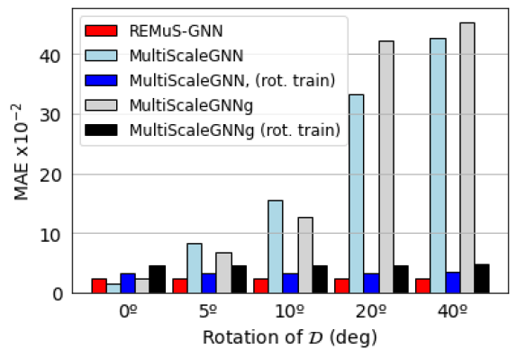
Figure 1: MAE ($\times 10^{-2}$) on the NsVal dataset under rotations of $\mathcal{D}$.

From Figure 1 it is clear that the MAEs of the predictions of MultiScaleGNN and MultiScaleGNNg trained without rotations grow significantly during inference on rotations of the domain greater than 5 degrees. On the other hand, these models trained with rotations are able to maintain an approximately constant MAE for each rotation of the domain. Hence, from now on we only consider these benchmark models. It can be seen that REMuS-GNN outperforms the benchmark models on every rotation of the validation dataset. Table 1 collects the MAE on the velocity field (measured with the free-stream as reference) and the MAE on the $x$-coordinate of the separation point on the upper wall of the ellipses. It can be concluded that REMuS-GNN also has a much better generalisation than the benchmark models. Additional results are included in Appendix E.

Table 1: MAE $\times 10^{-2}$ in the velocity field and the $x$-coordinate of the separation point

		NsLowRe	NsHighRe	NsThin	NsThick	NsNarrow	NsWide	NsAoA
REMuS-GNN	Velocity field	4.514	9.576	3.152	4.430	2.861	2.873	2.504
	Separation point	3.082	6.464	2.477	4.488	2.934	2.964	3.219
MultiScaleGNN	Velocity field	5.723	13.886	3.703	5.531	3.583	3.454	3.451
	Separation point	4.424	7.524	2.825	4.873	3.830	3.959	4.386
MultiScaleGNNg	Velocity field	4.826	8.552	4.085	7.201	4.759	4.666	4.593
	Separation point	4.414	7.264	3.025	6.405	4.222	4.468	4.993

5 Conclusion

We proposed a translation and rotational equivariant model for predicting the spatio-temporal evolution of vector fields defined on continuous domains, where the dynamics may encompass a range of length scales and/or be spatially global. The proposed model employs a generalised directional message-passing algorithm and a novel edge-unpooling algorithm specifically designed to satisfy the rotation invariance requirement. The incorporation of rotation equivariance as a strong inductive bias results in a higher accuracy and better generalisation compared with the vanilla data-augmentation approach for approximately learning the rotation equivariance. To the best of the authors’ knowledge, REMuS-GNN is the first multi-scale and rotation-equivariant GNN model for inferring Eulerian dynamics.

Appendix A Diagrams of REMuS-GNN’s building blocks

Appendix B Rotation invariance of the edge-unpooling layer

To achieve the rotation equivariance of REMuS-GNN it is required that the MP layers, edge-pooling layers and edge-unpooling layers are invariant to rotations. It is easy to see that MP and pooling layers (equations (4) to (6)) are rotation invariant. As for the unpooling from scale $\ell+1$ to scale $\ell$, the edge-unpooling layers in REMuS-GNN perform four steps:

1. Aggregation of the incoming-edges’ feature-vectors at each node in $V^{\ell+1}$ —equation (7).

2. Interpolation of the obtained features from $V^{\ell+1}$ to $V^{\ell}$ —knn-interpolation in (Qi et al., 2017).

3. Projection of the interpolated node-features along the direction of the incoming edges at scale $\ell$ —equation (8).

4. Update of the edge features —equation (9).

Steps 2 and 4 are invariant to rotations since they do not depend on the particular directions of the edges on $V^{\ell}$ nor $V^{\ell+1}$. On the other hand, step 1 is not rotation invariant since a two-dimensional rotation $\mathcal{R}:\bm{x}\rightarrow\bm{x}R$ of $\mathcal{D}$ (and $V^{1}$) modifies the output of the projection-aggregation function given by equation (3) to

$$([\hat{\bm{e}}^{\ell}_{1:\kappa,j}]R)^{+}[e_{1},e_{2},\dots,e_{\kappa}]^{T} =R^{+}[\hat{\bm{e}}^{\ell}_{1:\kappa,j}]^{+}[e_{1},e_{2},\dots,e_{\kappa}]^{T}$$

$$=R^{-1}\rho^{\ell+1}(e_{1},e_{2},\dots,e_{\kappa}).$$

Hence, according to equation (7), the result of the step 1 in the edge-unpooling layer is $R^{-1}W_{j}^{\ell+1}$ for all $j\in V^{\ell+1}$, and the result of step 2 (rotation invariant) is $R^{-1}W_{k}^{\ell}$ for all $k\in V^{\ell}$. Step 3 is not rotation invariant, and given the input $R^{-1}W_{k}^{\ell}$, the output that follows is

$$(\hat{\bm{e}}_{lk}^{\ell}R)(R^{-1}W_{k}^{\ell}) =\hat{\bm{e}}_{lk}^{\ell}W_{k}^{\ell}$$

$$=\bm{w}^{\ell}_{lk}.$$

Thus, despite step 1 and 3 are not invariant to rotations separately, they are when applied jointly.

Appendix C Datasets details

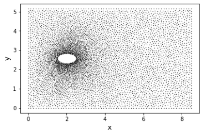
Figure 5: Set of nodes $V_{1}$ for a simulation on the Ns dataset.

We solved the two-dimensional incompressible Navier-Stokes equation using the high-order solver Nektar++ (Cantwell et al., 2015). The Navier-Stokes equations read

$$\frac{\partial u}{\partial x}+\frac{\partial v}{\partial y}=0,$$ (10)

$$\frac{\partial u}{\partial t}+u\frac{\partial u}{\partial x}+v\frac{\partial u}{\partial y}=-\frac{\partial p}{\partial x}+\frac{1}{Re}\bigg{(}\frac{\partial^{2}u}{\partial x^{2}}+\frac{\partial^{2}u}{\partial y^{2}}\bigg{)},$$ (11)

$$\frac{\partial v}{\partial t}+u\frac{\partial v}{\partial x}+v\frac{\partial v}{\partial y}=-\frac{\partial p}{\partial y}+\frac{1}{Re}\bigg{(}\frac{\partial^{2}v}{\partial x^{2}}+\frac{\partial^{2}v}{\partial y^{2}}\bigg{)},$$ (12)

where $u(t,x,y)$ and $v(t,x,y)$ are the horizontal and vertical components of the velocity field, $p(t,x,y)$ is the pressure field, and $Re$ is the Reynolds number. We consider the flow around an elliptical cylinder with major axis equal to one and minor axis $b$ on a rectangular fluid domain of dimensions $8.5\times D$ (see Figure 5). The left, top and bottom boundaries have as boundary condition $u=1$, $v=0$ and $\partial p/\partial x=0$; the right boundary is an outlet with $\partial u/\partial x=0$, $\partial v/\partial x=0$ and $p=0$; and the cylinder wall has a no-slip condition $u=v=0$. In our simulations we only selected $Re$ values that yield solutions within the laminar vortex-shedding regime. The sets of nodes $V^{1}$ employed for each simulation were created using Gmsh with an element-size equal to $h$ at the corners of the domain and $0.3h$ on the cylinder wall. Each simulation contains $100$ time-points equispaced by a time-step size $dt=0.1$. The parameters of the training, validation and testing datasets are collated in Table 2.

Table 2: Incompressible flow datasets

Dataset	$Re$	$b$	$H$	AoA (deg)	$h$	#Simulations	Purpose
Ns	500-1000	0.5-0.8	5-6	0	0.10-0.16	5000	Training
NsVal	500-1000	0.5-0.8	5-6	0	0.10-0.16	500	Validation
NsLowRe	200-500	0.5-0.8	5-6	0	0.10-0.16	500	Testing
NsHighRe	1000-1500	0.5-0.8	5-6	0	0.10-0.16	500	Testing
NsThin	500-1000	0.3-0.5	5-6	0	0.10-0.16	500	Testing
NsThick	500-1000	0.8-1.0	5-6	0	0.10-0.16	500	Testing
NsNarrow	500-1000	0.5-0.8	4-5	0	0.10-0.16	500	Testing
NsWide	500-1000	0.5-0.8	6-7	0	0.10-0.16	500	Testing
NsAoA	500-1000	0.5-0.8	5.5	0-10	0.12	240	Testing

Appendix D Models details

The implementation of the benchmark model MultiScaleGNN is taken from Lino et al. (2021). MultiScaleGNNg is a modified version of MultiScaleGNN to follow the pooling and unpooling used by Liu et al. (2021). For this model, the low-resolution sets of nodes were generated using Guillard’s coarsening algorithm (Guillard, 1993) as in REMuS-GNN. This way, both models share the same high and low-resolution discretisations. For a fair comparison all the models considered in the present work follow the same U-Net-like architecture and have in common the hyper-parameters and training setup described below. Hence, they have a similar number of learnable parameters ($\sim 2.2$M).

Hyper-parameters choice

The number of incoming edges at each node was set to $\kappa=5$, and the number of linear layers in each MLP is 2 (except for $f^{u}$, which has 3 linear layers), with 128 neurons per hidden layer. All MLPs use SELU activation functions (Klambauer et al., 2017), and, batch normalisation (Ba et al., 2016). The number of MP layers we used at each scale are $2\times M_{1}=8$, $2\times M_{2}=4$ and $M_{3}=4$.

Training details

During training four graphs were fed per iteration. First, each training iteration predicted a single time-point, and every time the training loss decreased below 0.02 we increased the number of iterative time-steps by one, up to a limit of 10. We used the loss function given by

$$\mathcal{L}=\mathrm{MSE} \Big{(}\hat{\mathbf{u}}(t,\mathbf{x}^{1}_{V^{1}}),\mathbf{u}(t,\mathbf{x}^{1}_{V^{1}})\Big{)}$$

$$+\lambda_{d}\,\mathrm{MAE}\Big{(}\hat{\mathbf{u}}(t,{\mathbf{x}^{1}_{V^{1}}\in\partial_{D}\mathcal{D}}),\mathbf{u}(t,\mathbf{x}^{1}_{V^{1}}\in\partial_{D}\mathcal{D})\Big{)},$$

with $\lambda_{d}=0.25$. The initial time-point $t_{0}$ was randomly selected for each prediction, and, we added to the initial field noise following a uniform distribution between -0.01 and 0.01. After each time-step, the models’ weights were updated using the Adam optimiser with its standard parameters (Kingma & Ba, 2015). The learning rate was set to $10^{-4}$ and multiplied by 0.5 when the training loss did not decrease after two consecutive epochs, also, we applied gradient clipping to keep the Frobenius norm of the weights’ gradients below or equal to one.

Appendix E Additional results

REMuS-GNN is rotation equivariant by design, whereas traditionally this symmetry is learnt through data augmentation of the training dataset with random rotations of the physical domain. Figure 6 shows the ground truth and predictions after 100 time-steps of the horizontal velocity on a sample from the NsVal dataset that has been rotated 10 degrees. It can be observed that the benchmark models trained without rotations produce unstable simulations, whereas all the other models produce realistic results. Among these, REMuS-GNN has the lower MAE and produces a better resolved solution. Figure 7 shows the ground truth and predictions after 100 time-steps of the horizontal velocity on a sample from the NsAoA dataset. In this case the ellipse has been rotated 10 degrees clockwise (i.e. the angle of attack is 10 degrees). It is possible to notice that in REMuS-GNN’s prediction the position of the wake and vortices, as well as their shape, is more similar to the ground truth than in the other two benchmark models (both trained with rotations). This illustrates the better generalisation of REMuS-GNN with respect to models that are not designed to be rotation equivariant. Simulations with the ground truth and predictions of REMuS-GNN and the benchmark models can be found here.

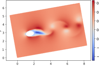
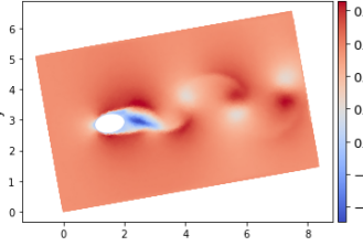
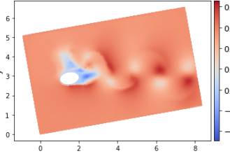
(a) Target	(b) REMuS-GNN	(c) MultiScaleGNN
	(MAE = 0.0210)	train no rots. (MAE = 0.1051)
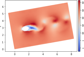
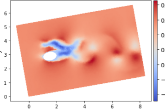
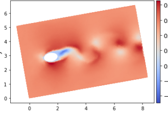
(d) MultiScaleGNN	(e) MultiScaleGNNg	(f) MultiScaleGNNg
train rots. (MAE = 0.0245)	train no rots. (MAE = 0.0997)	train rots. (MAE = 0.0587)

Figure 6: Target and predictions (after 100 time-steps) of the horizontal velocity field with a rotation of 10 degrees of the physical domain (sample from the validation dataset NsVal with $Re=864$).

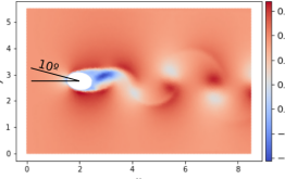
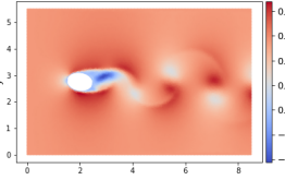
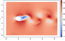
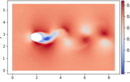
(a) Target	(b) REMuS-GNN	(c) MultiScaleGNN	(d) MultiScaleGNNg
	(MAE = 0.0148)	(MAE = 0.0223)	(MAE = 0.0735)

Figure 7: Target and predictions (after 100 time-steps) of the horizontal velocity field around an ellipse with an angle of attack of 10º and $Re=800$ (sample from the NsAoA dataset).

References

- Alet et al. (2019) Ferran Alet, Adarsh Keshav Jeewajee, Maria Bauza Villalonga, Alberto Rodriguez, Tomas Lozano-Perez, and Leslie Kaelbling. Graph element networks: adaptive, structured computation and memory. In International Conference on Machine Learning, pp. 212–222. PMLR, 2019.
- Ba et al. (2016) Jimmy Lei Ba, Jamie Ryan Kiros, and Geoffrey E Hinton. Layer normalization. arXiv preprint arXiv:1607.06450, 2016.
- Battaglia et al. (2018) Peter W Battaglia, Jessica B Hamrick, Victor Bapst, Alvaro Sanchez-Gonzalez, Vinicius Zambaldi, Mateusz Malinowski, Andrea Tacchetti, David Raposo, Adam Santoro, Ryan Faulkner, et al. Relational inductive biases, deep learning, and graph networks. arXiv preprint arXiv:1806.01261, 2018.
- Cantwell et al. (2015) Chris D Cantwell, David Moxey, Andrew Comerford, Alessandro Bolis, Gabriele Rocco, Gianmarco Mengaldo, Daniele De Grazia, Sergey Yakovlev, J-E Lombard, Dirk Ekelschot, et al. Nektar++: An open-source spectral/hp element framework. Computer physics communications, 192:205–219, 2015.
- Chen et al. (2021) J Chen, E Hachem, and J Viquerat. Graph neural networks for laminar flow prediction around random two-dimensional shapes. Physics of Fluids, 33(12):123607, 2021.
- Chu & Thuerey (2017) Mengyu Chu and Nils Thuerey. Data-driven synthesis of smoke flows with cnn-based feature descriptors. ACM Transactions on Graphics (TOG), 36(4):1–14, 2017.
- Fuchs et al. (2020) Fabian Fuchs, Daniel Worrall, Volker Fischer, and Max Welling. Se (3)-transformers: 3d roto-translation equivariant attention networks. Advances in Neural Information Processing Systems, 33:1970–1981, 2020.
- Guillard (1993) Hervé Guillard. Node-nested multi-grid method with delaunay coarsening. Technical report, INRIA, 1993.
- Guo et al. (2016) Xiaoxiao Guo, Wei Li, and Francesco Iorio. Convolutional neural networks for steady flow approximation. In Proceedings of the 22nd ACM SIGKDD international conference on knowledge discovery and data mining, pp. 481–490, 2016.
- Karniadakis & Sherwin (2013) George Karniadakis and Spencer Sherwin. Spectral/hp element methods for computational fluid dynamics. Oxford University Press, 2013.
- Kim et al. (2019) Byungsoo Kim, Vinicius C Azevedo, Nils Thuerey, Theodore Kim, Markus Gross, and Barbara Solenthaler. Deep fluids: A generative network for parameterized fluid simulations. In Computer Graphics Forum. Wiley Online Library, 2019.
- Kingma & Ba (2015) Diederik P. Kingma and Jimmy Ba. Adam: A method for stochastic optimization. In Yoshua Bengio and Yann LeCun (eds.), 3rd International Conference on Learning Representations, ICLR 2015, San Diego, CA, USA, May 7-9, 2015, Conference Track Proceedings, 2015. URL http://arxiv.org/abs/1412.6980.
- Klambauer et al. (2017) Günter Klambauer, Thomas Unterthiner, Andreas Mayr, and Sepp Hochreiter. Self-normalizing neural networks. arXiv preprint arXiv:1706.02515, 2017.
- Klicpera et al. (2020) Johannes Klicpera, Janek Groß, and Stephan Günnemann. Directional message passing for molecular graphs. In 8th International Conference on Learning Representations, ICLR 2020, 2020.
- Klicpera et al. (2021a) Johannes Klicpera, Florian Becker, and Stephan Günnemann. Gemnet: Universal directional graph neural networks for molecules. Advances in Neural Information Processing Systems, 34, 2021a.
- Klicpera et al. (2021b) Johannes Klicpera, Chandan Yeshwanth, and Stephan Günnemann. Directional message passing on molecular graphs via synthetic coordinates. Advances in Neural Information Processing Systems, 34, 2021b.
- Lee & You (2019) Sangseung Lee and Donghyun You. Data-driven prediction of unsteady flow over a circular cylinder using deep learning. Journal of Fluid Mechanics, 879:217–254, 2019.
- Li et al. (2019) Yunzhu Li, Jiajun Wu, Russ Tedrake, Joshua B Tenenbaum, and Antonio Torralba. Learning particle dynamics for manipulating rigid bodies, deformable objects, and fluids. In 7th International Conference on Learning Representations, ICLR 2019, 2019.
- Li et al. (2020) Zongyi Li, Nikola Kovachki, Kamyar Azizzadenesheli, Burigede Liu, Andrew Stuart, Kaushik Bhattacharya, and Anima Anandkumar. Multipole graph neural operator for parametric partial differential equations. Advances in Neural Information Processing Systems, 33:6755–6766, 2020.
- Lino et al. (2021) Mario Lino, Chris Cantwell, Anil A Bharath, and Stathi Fotiadis. Simulating continuum mechanics with multi-scale graph neural networks. arXiv preprint arXiv:2106.04900, 2021.
- Liu et al. (2021) Wenzhuo Liu, Mouadh Yagoubi, and Marc Schoenauer. Multi-resolution graph neural networks for pde approximation. In International Conference on Artificial Neural Networks, pp. 151–163. Springer, 2021.
- Liu et al. (2022) Yi Liu, Limei Wang, Meng Liu, Yuchao Lin, Xuan Zhang, Bora Oztekin, and Shuiwang Ji. Spherical message passing for 3d molecular graphs. In 10th International Conference on Learning Representations, ICLR 2022, 2022.
- Mrowca et al. (2018) Damian Mrowca, Chengxu Zhuang, Elias Wang, Nick Haber, Li F Fei-Fei, Josh Tenenbaum, and Daniel L Yamins. Flexible neural representation for physics prediction. In Advances in neural information processing systems, pp. 8799–8810, 2018.
- Özbay et al. (2019) Ali Girayhan Özbay, Sylvain Laizet, Panagiotis Tzirakis, Georgios Rizos, and Björn Schuller. Poisson CNN: Convolutional Neural Networks for the Solution of the Poisson Equation with Varying Meshes and Dirichlet Boundary Conditions, 2019. URL http://arxiv.org/abs/1910.08613.
- Pfaff et al. (2021) Tobias Pfaff, Meire Fortunato, Alvaro Sanchez-Gonzalez, and Peter W Battaglia. Learning mesh-based simulation with graph networks. In (accepted) 38th International Conference on Machine Learning, ICML 2021, 2021.
- Qi et al. (2017) Charles Ruizhongtai Qi, Li Yi, Hao Su, and Leonidas J Guibas. Pointnet++: Deep hierarchical feature learning on point sets in a metric space. Advances in neural information processing systems, 30, 2017.
- Sanchez-Gonzalez et al. (2018) Alvaro Sanchez-Gonzalez, Nicolas Heess, Jost Tobias Springenberg, Josh Merel, Martin Riedmiller, Raia Hadsell, and Peter Battaglia. Graph networks as learnable physics engines for inference and control. 35th International Conference on Machine Learning, ICML 2018, 10:7097–7117, 2018.
- Satorras et al. (2021) Victor Garcia Satorras, Emiel Hoogeboom, and Max Welling. E (n) equivariant graph neural networks. In International Conference on Machine Learning, pp. 9323–9332. PMLR, 2021.
- Schütt et al. (2021) Kristof Schütt, Oliver Unke, and Michael Gastegger. Equivariant message passing for the prediction of tensorial properties and molecular spectra. In International Conference on Machine Learning, pp. 9377–9388. PMLR, 2021.
- Siddani et al. (2021) B Siddani, S Balachandar, and Ruogu Fang. Rotational and reflectional equivariant convolutional neural network for data-limited applications: Multiphase flow demonstration. Physics of Fluids, 33(10):103323, 2021.
- Tang et al. (2018) Wei Tang, Tao Shan, Xunwang Dang, Maokun Li, Fan Yang, Shenheng Xu, and Ji Wu. Study on a Poisson’s equation solver based on deep learning technique. 2017 IEEE Electrical Design of Advanced Packaging and Systems Symposium, EDAPS 2017, 2018-Janua:1–3, 2018. doi: 10.1109/EDAPS.2017.8277017.
- Thomas et al. (2018) Nathaniel Thomas, Tess Smidt, Steven Kearnes, Lusann Yang, Li Li, Kai Kohlhoff, and Patrick Riley. Tensor field networks: Rotation-and translation-equivariant neural networks for 3d point clouds. arXiv preprint arXiv:1802.08219, 2018.
- Thuerey et al. (2018) Nils Thuerey, Konstantin Weissenow, Lukas Prantl, and Xiangyu Hu. Deep Learning Methods for Reynolds-Averaged Navier-Stokes Simulations of Airfoil Flows. AIAA Journal, 58(1):15–26, oct 2018. ISSN 0001-1452. doi: 10.2514/1.j058291. URL http://arxiv.org/abs/1810.08217.
- Wang et al. (2021) Rui Wang, Robin Walters, and Rose Yu. Incorporating symmetry into deep dynamics models for improved generalization. In 9th International Conference on Learning Representations, ICLR 2021, 2021.
- Weiler & Cesa (2019) Maurice Weiler and Gabriele Cesa. General e (2)-equivariant steerable cnns. Advances in Neural Information Processing Systems, 32, 2019.
- Weiler et al. (2018) Maurice Weiler, Mario Geiger, Max Welling, Wouter Boomsma, and Taco S Cohen. 3d steerable cnns: Learning rotationally equivariant features in volumetric data. Advances in Neural Information Processing Systems, 31, 2018.
- Wiewel et al. (2019) Steffen Wiewel, Moritz Becher, and Nils Thuerey. Latent space physics: Towards learning the temporal evolution of fluid flow. In Computer Graphics Forum. Wiley Online Library, 2019.