AdaCap: Adaptive Capacity control for Feed-Forward Neural Networks

Abstract

The capacity of a ML model refers to the range of functions this model can approximate. It impacts both the complexity of the patterns a model can learn but also memorization, the ability of a model to fit arbitrary labels. We propose Adaptive Capacity (AdaCap), a training scheme for Feed-Forward Neural Networks (FFNN). AdaCap optimizes the $capacity$ of FFNN so it can capture the high-level abstract representations underlying the problem at hand without memorizing the training dataset. AdaCap is the combination of two novel ingredients, the Muddling labels for Regularization (MLR) loss and the Tikhonov operator training scheme. The MLR loss leverages randomly generated labels to quantify the propensity of a model to memorize. We prove that the MLR loss is an accurate in-sample estimator for out-of-sample generalization performance and that it can be used to perform Hyper-Parameter Optimization provided a Signal-to-Noise Ratio condition is met. The Tikhonov operator training scheme modulates the $capacity$ of a FFNN in an adaptive, differentiable and data-dependent manner. We assess the effectiveness of AdaCap in a setting where DNN are typically prone to memorization, small tabular datasets, and benchmark its performance against popular machine learning methods.

1 Introduction

Generalization is a central problem in Deep Learning (DL). It is strongly connected to the notion of capacity of a model, that is the range of functions a model can approximate. It impacts both the complexity of the patterns a model can learn but also memorization, the ability of a model to fit arbitrary labels (Goodfellow et al., 2016). Because of their high capacity, overparametrized Deep Neural Networks (DNN) can memorize the entire train set to the detriment of generalization. Common techniques like Dropout (DO) (Hinton et al., 2012; Srivastava et al., 2014), Early Stopping (Li et al., 2020), Data Augmentation (Shorten & Khoshgoftaar, 2019) or Weight Decay (Hanson & Pratt, 1988; Krogh & Hertz, 1992; Bos & Chug, 1996) used during training can reduce the capacity of a DNN and sometimes delay memorization but cannot prevent it (Arpit et al., 2017).

We propose AdaCap, a new training technique for Feed-Forward Neural Networks (FFNN) that optimizes the $capacity$ of FFNN during training so that it can capture the high-level abstract representations underlying the problem at hand and mitigate memorization of the train set. AdaCap relies on two novel ingredients, the Tikhonov operator and the Muddling labels Regularization (MLR) loss.

The Tikhonov operator provides a differentiable data-dependent quantification of the capacity of a FFNN through the application of this operator on the output of the last hidden layer. The Tikhonov operator modulates the capacity of the FFNN via the additional Tikhonov parameter that can be trained concomitantly with the hidden layers weights by Gradient Descent (GD). This operator works in a fundamentally different way from other existing training techniques like Weight Decay (See Section 3 and Fig. 1).

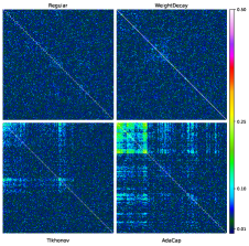
Figure 1: We trained a MLP on the Boston dataset with either usual training (with/without Weight Decay) or AdaCap, using identical architectures and parameters in both cases. We plot the clustered correlation matrices of last hidden layer weights (in absolute value). Upper left: usual loss and no regularization. Upper right: usual loss and Weight Decay only. Bottom left: usual loss and Tikhonov scheme alone (no Weight Decay). Bottom right: AdaCap alone. Contrarily to Weight Decay, AdaCap produced a model with highly structured hidden layer weights even with a plain MLP architecture, indicating its learning behavior is very different from the standard one.

The problem is then the tuning of the Tikhonov parameter that modulates capacity as it directly impacts the generalization performance of the trained FFNN. This motivated the introduction of the MLR loss which performs capacity tuning without using a hold-out validation set. The MLR loss is based on a novel way to exploit random labels.

Random labels have been used in (Zhang et al., 2016; Arpit et al., 2017) as a diagnostic tool to understand how overparametrized DNN can generalize surprisingly well despite their capacity to memorise the train set. This benign overfitting phenonemon is attributed in part to the implicit regularization effect of the optimizer schemes used during training (Gunasekar et al., 2018; Smith et al., 2021). Understanding that the training of DNN is extremely susceptible to corrupted labels, numerous methods have been proposed to identify the noisy labels or to reduce their impact on generalization. These approaches include loss correction techniques (Patrini et al., 2017), reweighing samples (Jiang et al., 2017), training two networks in parallel (Han et al., 2018). See (Chen et al., 2019; Harutyunyan et al., 2020) for an extended survey.

We propose a different approach. We do not attempt to address the noise and corruptions already present in the original labels. Instead, we purposely generate purely corrupted labels during training as a tool to reduce the propensity of the DNN to memorize label noise during gradient descent. The underlying intuition is that we no longer see generalization as the ability of a model to perform well on unseen data, but rather as the ability to avoid finding pattern where none exists. Concretely, we propose the Muddling labels Regularization loss which uses randomly permuted labels to quantify the overfitting ability of a model on a given dataset. In Section 2, we provide theoretical evidences in a regression setting that the MLR loss is an accurate estimator of the generalization error (Fig. 4) which can be used to perform Hyper-Parameter Optimization (HPO) without using a hold-out $validation$-set if a Signal-to-Noise Ratio (SNR) condition is satisfied.

This property motivates using the MLR loss rather than the usual losses during training to perform $adaptive$ control of the $capacity$ of DNN. This can improve generalization (Fig. 2) not only in the presence of label corruption but also in other settings prone to overfitting - $e.g.$ Tabular Data (Borisov et al., 2021; Gorishniy et al., 2021; Shwartz-Ziv & Armon, 2022), Few-Shot Learning (Fig. 3), a task introduced in (Fink, 2005; Fei-Fei et al., 2006). See (Wang et al., 2020) for a recent survey.

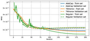
Figure 2: RMSE across iterations for train and valid sets when training AdaCap, Tikhonov and regular DNN on Abalone TD. We can see the improvement in terms of generalization and memorization when adding Tikhonov and then MLR: The train RMSE converges to a higher plateau but validation RMSE keeps improving further. Tikhonov smooths the learning dynamic, removes the oscillations. Adding the MLR loss makes no change to the learning dynamic on the first iterations but impact the last iterations and delays memorization even more.

Our novel training method AdaCap works as follows. Before training: a) generate a new set of completely uninformative labels by muddling original labels through random permutations; then, at each GD iteration: b) apply the Tikhonov operator to the output of the last hidden layer; c) quantify the ability of the DNN’s output layer to fit true labels rather than permuted labels via the new (MLR) loss; d) back-propagate the MLR objective through the network.

AdaCap is a gradient-based, global, data-dependent method which trains the weights and adjusts the capacity of the FFNN simultaneously during the training phase without using a hold-out $validation$ set. AdaCap is designed to work on most FFNN architectures and is compatible with the usual training techniques like Gradient Optimizers (Kingma & Ba, 2014), Learning Rate Schedulers (Smith & Topin, 2019), Dropout (Srivastava et al., 2014), Batch-Norm (Ioffe & Szegedy, 2015), Weight Decay (Krogh & Hertz, 1992; Bos & Chug, 1996), etc.

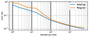
Figure 3: Few-shot learning experiment on MNIST (Deng, 2012). When training a simple ConvNet, the generalization performance of the obtained models $w.r.t.$ the number of samples per class is uniformly better over the whole range of samples per class when using AdaCap, especially in the low sample per class regime.

DNN have not demonstrated yet the same level of success on Tabular Data (TD) as on images (Krizhevsky et al., 2012), audio (Hinton et al., 2012) and text (Devlin et al., 2019), which makes it an interesting frontier for DNN architectures. Due to the popularity of tree-based ensemble methods (CatBoost (Prokhorenkova et al., 2018), XGBoost (Chen & Guestrin, 2016), RF (Barandiaran, 1998; Breiman, 2001)), there has been a strong emphasis on the preprocessing of categorical features which was an historical limitation of DL. Notable contributions include NODE (Popov et al., 2020) and TabNet (Arik & Pfister, 2020). NODE (Neural Oblivious Decision Ensembles) are tree-like architectures which can be trained end-to-end via backpropagation. TabNet leverages Attention Mechanisms (Bahdanau et al., 2014) to pretrain DNN with feature encoding. The comparison between simple DNN, NODE, TabNet, RF and GBDT on TD was made concomitantly by Kadra et al. (2021), Gorishniy et al. (2021) and Shwartz-Ziv & Armon (2022). Their benchmarks are more oriented towards an AutoML approach than ours, as they all use heavy HPO, and report training times in minutes/hours, even for some small and medium size datasets. See Appendix C for a more detailed discussion. As claimed by (Shwartz-Ziv & Armon, 2022), their results (like ours) indicate that DNN are not (yet?) the alpha and the omega of TD. (Kadra et al., 2021) also introduces an HPO strategy called the regularization cocktail. Regarding the new techniques for DNN on TD, we mention here a few relevant to our work which we included in our benchmark. See (Borisov et al., 2021) and the references therein for a more exhaustive list. (Klambauer et al., 2017) introduced Self-Normalizing Networks (SNN) to train deeper FFNN models, leveraging the SeLU activation function. Gorishniy et al.(2021) proposed new architecture schemes: ResBlock, Gated Linear Units GLU, and FeatureTokenizer-Transformers, which are adaptation for TD of ResNet (He et al., 2016), Gated convolutional networks (Dauphin et al., 2017) and Transformers (Vaswani et al., 2017).

We illustrate the potential of AdaCap on a benchmark of 44 tabular datasets from diverse domains of application, including 26 regression tasks, 18 classification tasks, against a large set of popular methods GBDT (Breiman, 1997; Friedman, 2001, 2002; Chen & Guestrin, 2016; Ke et al., 2017; Prokhorenkova et al., 2018); Decision Trees and RF (Breiman et al., 1984; Barandiaran, 1998; Breiman, 2001; Gey & Nedelec, 2005; Klusowski, 2020), Kernels (Chang & Lin, 2011), MLP (Hinton, 1989), GLM (Cox, 1958; Hoerl & Kennard, 1970; Tibshirani, 1996; Zou & Hastie, 2005), MARS (Friedman, 1991)).

For DL architectures, we combined and compared AdaCap with MLP, GLU, ResBlock, SNN and CNN. We left out recent methods designed to tackle categorical features (TabNet, NODE, FT-Transformers) as it is not the focus of this benchmark and of our proposed method. Our experimental study reveals that using AdaCap to train FFNN leads to an improvement of the generalization performance on regression tabular datasets especially those with high Signal-to-Noise Ratio (SNR), the datasets where it is possible but not trivial to obtain a very small test RMSE. AdaCap works best in combination with other schemes and architectures like SNN, GLU or ResBlock. Introducing AdaCap to the list of available DNN schemes allows neural networks to gain ground against the GBDT family.

2 The MLR loss

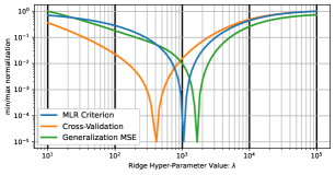
Figure 4: Comparison of the MLR criterion (blue), CV criterion ($10$-Fold cross-validation RMSE) (orange) for out-of-sample performance (test set RMSE) (green) estimation with the Ridge model. We generated synthetic regression data (Appendix A.1), and train a Ridge model with different levels of regularization $\lambda$. We also train a Ridge model with a randomly permuted target vector. We evaluate the MLR criterion, the $10$-Fold CV RMSE and test RMSE over the $\lambda$ grid and compare their respective argmin, $\widehat{\lambda}_{{\texttt{MLR}}}$, $\widehat{\lambda}_{\texttt{CV}}$ and $\lambda^{*}$. The goal is to obtain an argmin as close as possible to the optimal one in terms of generalization. Averaging over $100$ seeds, the RMSE test performances with $\widehat{\lambda}_{{\texttt{MLR}}}$, $\widehat{\lambda}_{\texttt{CV}}$ and $\lambda^{*}$ are $0.7128$, $0.7221$ and $0.7061$ respectively. Above figure is the criterion landscape for random seed $0$. We see that MLR provides a better estimate of the argmin of test RMSE than CV.

Setting. Let $\mathcal{D}_{train}=(\textbf{x},\textbf{Y})=\{(\textbf{x}_{i},Y_{i})\}_{i=1}^{n}$ be the $train$-set with $\textbf{x}_{i}\in\mathbb{R}^{d}$ where $d$ denotes the number of features and $Y_{i}\in\mathcal{Y}$ where $\mathcal{Y}=\mathbb{R}$ for regression and $\mathcal{Y}$ is a finite set for classification. We optimise the objective $L(\texttt{act}_{\texttt{out}}(\bm{f}_{\bm{\theta}}(\textbf{x})),\textbf{Y})$ where $\bm{f}_{\bm{\theta}}(\textbf{x})$ is the output of the last hidden layer, $L$ is the loss function (MSE for regression and CE for classification) and $\texttt{act}_{\texttt{out}}$ is the activation function (Id for regression, Sigmoid for binary classification and logsoftmax for multiclass).

Random permutations.We build a randomized data set by applying random permutations on the $n$ components of the label vector Y. This randomization scheme presents the advantage of creating an artificial train set $(\textbf{x},\textbf{Y}_{\texttt{perm}})$ with marginal distributions of features and labels identical to those in the initial train set but where the connection between features and labels has been removed. This means that there is no generalizing pattern to learn from the artificial dataset $(\textbf{x},\textbf{Y}_{\texttt{perm}})$. We replace the initial loss $L$ by

$${\texttt{MLR}}(\bm{\theta}):=L\left(\textbf{Y},\texttt{act}_{\texttt{out}}(\bm{f}_{\bm{\theta}}(\textbf{x}))\right)$$

$$\hskip 56.9055pt-L\left(\textbf{Y}_{\texttt{perm}},\texttt{act}_{\texttt{out}}(\bm{f}_{\bm{\theta}}(\textbf{x}))\right).$$ (1)

The second term on the right-hand side of (1) is used to quantify memorization of output layer $\bm{f}_{\bm{\theta}}$. Indeed, since there is no meaningful pattern linking x to $\textbf{Y}_{\texttt{perm}}$, any $\bm{f}_{\bm{\theta}}$ which fits $(\textbf{x},\textbf{Y}_{\texttt{perm}})$ well achieves it via memorization only. We want to rule out such models. By minimizing the MLR loss, we hope to retain only the generalizing patterns.

The MLR approach uses random labels in an original way. In (Zhang et al., 2016; Arpit et al., 2017), noise labels are used as a diagnostic tool in numerical experiments. On the theory side, Rademacher Process (RP) is a central tool exploiting random (Rademacher) labels to compute data dependent measures of complexity of function classes used in learning (Koltchinskii, 2011). However, RP are used to derive bounds on the excess risk of already trained models whereas the MLR approach uses randomly permuted labels to train the model.

Experiment (Fig.4). We compare the MLR loss and Cross-Validation (CV) error to the true generalization error in the correlated regression setting described in Appendix A.1. MLR is a better estimate of the generalization error than CV, thus yielding a more precise estimate of the optimal hyperparameter $\lambda^{*}$ than CV.

Theoretical investigation of MLR. To understand the core mechanism behind the MLR loss, we consider the following toy regression model. Let $\textbf{Y}=\textbf{x}\bm{\beta}^{*}+\bm{\xi}$ with $\bm{\beta}^{*}\in\mathbb{R}^{d}$ and isotropic sub-Gaussian noise $\bm{\xi}\in\mathbb{R}^{n}$ ($\mathrm{Cov}(\bm{\xi})=\sigma^{2}\mathbb{I}_{n}$). We consider the class of Ridge models $\mathcal{F}^{R}=\{f_{\lambda}(\cdot)=\langle\bm{\beta}_{\lambda},\cdot\rangle,\;\lambda>0\}$ with $\bm{\beta}_{\lambda}=\bm{\beta}_{\lambda}(\textbf{x},\textbf{Y})=(\textbf{x}^{\top}\textbf{x}+\lambda\mathbb{I}_{d})^{-1}\textbf{x}^{\top}\textbf{Y}\in\mathbb{R}^{d}$. Define the risk $R(\lambda):=\mathbb{E}_{\bm{\xi}}[\|\textbf{x}\bm{\beta}^{*}-\textbf{x}\bm{\beta}_{\lambda}\|_{2}^{2}]$, and the optimal parameter $\lambda^{*}=\mathrm{argmin}_{\lambda>0}R(\lambda)$. We assume for simplicity that $\textbf{x}^{\top}\textbf{x}/n$ is an orthogonal projection (denoted $P_{\textbf{x}}$) onto a $r$-dimensional subspace of $\mathbb{R}^{d}$. Define the rate

$$\epsilon_{n}:=\sqrt{\frac{r\sigma^{2}}{\|\textbf{x}\bm{\beta}^{*}\|_{2}^{2}}}+\sqrt{\frac{\|\textbf{x}\bm{\beta}^{*}\|_{2}^{2}}{n\sigma^{2}}}.$$

Theorem 2.1.

Under the above assumptions. If $r\sigma^{2}\ll\|\textbf{x}\bm{\beta}^{*}\|_{2}^{2}\ll n\sigma^{2}$, then we get w.h.p.

$${\texttt{MLR}}(\lambda)+\|P_{\textbf{x}}(\textbf{Y}_{\texttt{perm}})\|_{2}^{2}=\left(1+o(1)\right)R(\lambda),\quad\forall\lambda>\epsilon_{n}.$$

Proof is provided in Appendix A.2. In our setting, $\|\textbf{x}\bm{\beta}^{*}\|_{2}^{2}/(n\sigma^{2})$ is the Signal-to-Noise Ratio SNR. The intermediate SNR regime $r\sigma^{2}\ll\|\textbf{x}\bm{\beta}^{*}\|_{2}^{2}\ll n\sigma^{2}$ is the only regime where using Ridge regularization can yield a significant improvement in the prediction. In that regime, the MLR loss can be used to find optimal hyperparameter $\lambda^{*}$. In the high SNR regime $\|\textbf{x}\bm{\beta}^{*}\|_{2}^{2}\geq n\sigma^{2}$, no regularization is needed, i.e. $\lambda^{*}=0$ is the optimal choice. Conversely in the low SNR regime $\|\textbf{x}\bm{\beta}^{*}\|_{2}^{2}\leq r\sigma^{2}$, the signal is completely drowned in the noise. Consequently it is better to use the zero estimator, i.e. $\lambda^{*}=\infty$.
In a nutshell, while the high and low SNR regimes correspond to trivial cases where regularization is not useful, in the intermediate regime where regularization is beneficial, MLR is useful.

3 The AdaCap method to train DNN

The Tikhonov operator scheme. Consider a DNN architecture with $L$ layers. Denote by $\bm{\theta}$ the hidden layers weights and by $\textbf{A}^{L-1}(\bm{\theta},\mathchoice{\mathbin{\vbox{\hbox{\scalebox{0.5}{$\displaystyle\bullet$}}}}}{\mathbin{\vbox{\hbox{\scalebox{0.5}{$\textstyle\bullet$}}}}}{\mathbin{\vbox{\hbox{\scalebox{0.5}{$\scriptstyle\bullet$}}}}}{\mathbin{\vbox{\hbox{\scalebox{0.5}{$\scriptscriptstyle\bullet$}}}}})\,:\,\mathbb{R}^{n\times d}\rightarrow\mathbb{R}^{n\times d_{L-1}}$ the output of the last hidden layer.
Let $\lambda\in\mathbb{R}_{+}^{*}$ be the Tikhonov parameter and define

$$\textbf{P}(\lambda,\bm{\theta},\textbf{x}):=\left[\left(\textbf{A}^{L-1}\right)^{\top}\textbf{A}^{L-1}+\lambda\mathbb{I}\right]^{-1}\left(\textbf{A}^{L-1}\right)^{\top}$$ (2)

where $\textbf{A}^{L-1}:=A^{L-1}(\bm{\theta},\textbf{x})$ and $\mathbb{I}=\mathbb{I}_{d_{L-1}}$ the identity matrix. The Tikhonov operator is

$$\textbf{H}(\lambda,\bm{\theta},\textbf{x}):=\textbf{A}^{L-1}\textbf{P}(\lambda,\bm{\theta},\textbf{x}).$$ (3)

During training, the Tikhonov operator scheme outputs the following prediction for target vector Y:

$$\bm{f}_{\lambda,\bm{\theta},\textbf{Y}}(\textbf{x})=\textbf{H}(\lambda,\bm{\theta},\textbf{x})\textbf{Y},$$ (4)

Note that $(\lambda,\bm{\theta},\textbf{x},\textbf{Y})$ may change at each iteration during training/GD. To train this DNN, we run a Gradient Descent Optimization scheme over parameters $(\lambda,\bm{\theta})$

$$(\widehat{\lambda},\widehat{\bm{\theta}})=\underset{\lambda>0,\,\bm{\theta}}{\arg\min}\;L\left(\textbf{Y},\texttt{act}_{\texttt{out}}\left(\bm{f}_{\lambda,\bm{\theta},\textbf{Y}}(\textbf{x})\right)\right).$$ (5)

Eventually, at test time, we freeze $\textbf{P}(\widehat{\lambda},\widehat{\bm{\theta}},\textbf{x})$, and obtain our final predictor

$$\bm{f}_{\widehat{\lambda},\widehat{\bm{\theta}}}(\mathchoice{\mathbin{\vbox{\hbox{\scalebox{0.5}{$\displaystyle\bullet$}}}}}{\mathbin{\vbox{\hbox{\scalebox{0.5}{$\textstyle\bullet$}}}}}{\mathbin{\vbox{\hbox{\scalebox{0.5}{$\scriptstyle\bullet$}}}}}{\mathbin{\vbox{\hbox{\scalebox{0.5}{$\scriptscriptstyle\bullet$}}}}})=\texttt{act}_{\texttt{out}}\left(A^{L-1}(\widehat{\bm{\theta}},\mathchoice{\mathbin{\vbox{\hbox{\scalebox{0.5}{$\displaystyle\bullet$}}}}}{\mathbin{\vbox{\hbox{\scalebox{0.5}{$\textstyle\bullet$}}}}}{\mathbin{\vbox{\hbox{\scalebox{0.5}{$\scriptstyle\bullet$}}}}}{\mathbin{\vbox{\hbox{\scalebox{0.5}{$\scriptscriptstyle\bullet$}}}}})\textbf{P}(\widehat{\lambda},\widehat{\bm{\theta}},\textbf{x})\textbf{Y}\right),$$ (6)

where $\texttt{act}_{\texttt{out}}$ is the last activation function applied to the output layer. Here, $\textbf{P}(\widehat{\lambda},\widehat{\bm{\theta}},\textbf{x})\textbf{Y}$ are the weights of the output layer set once and for all using the minibatch (x, Y) associated with ($\widehat{\lambda},\widehat{\bm{\theta}}$) in case of batch-learning. Therefore, we recover the architecture of a standard DNN where the output of the hidden layers $A^{L-1}(\widehat{\bm{\theta}},\mathchoice{\mathbin{\vbox{\hbox{\scalebox{0.5}{$\displaystyle\bullet$}}}}}{\mathbin{\vbox{\hbox{\scalebox{0.5}{$\textstyle\bullet$}}}}}{\mathbin{\vbox{\hbox{\scalebox{0.5}{$\scriptstyle\bullet$}}}}}{\mathbin{\vbox{\hbox{\scalebox{0.5}{$\scriptscriptstyle\bullet$}}}}})$ is multiplied by the weights of the output layer.

The Tikhonov operator scheme works in a fundamentally different way from Weight Decay. When we apply the Tikhonov operator to the output of the last hidden layer and then use backpropagation to train the DNN, we are indirectly carrying over its $capacity$ control effect to the hidden layers of the DNN. In other words, we are performing inter-layers regularization (i.e. regularization across the hidden layers) whereas Weight Decay performs intra-layer regularization. We trained a DNN using Weight Decay on the one-hand and Tikhonov operator on the other hand while all the other training choices were the same between the two training schemes (same loss $L$, same architecture size, same initialization, same learning rate, etc.). Fig. 1 shows that the Tikhonov scheme works differently from other $L_{2}$ regularization schemes like Weight Decay. Indeed, Fig.  2 reveals that the Tikhonov scheme completely changes the learning dynamic during GD.

Training with MLR loss and the Tikhonov scheme. We quantify the $capacity$ of our model to memorize labels Y by $L\left(\textbf{Y},\texttt{act}_{\texttt{out}}\left(\bm{f}_{\lambda,\bm{\theta},\textbf{Y}}(\textbf{x})\right)\right)$ w.r.t. to labels Y where the Tikhonov parameter $\lambda$ modulates the level the $capacity$ of this model. However, we are not so much interested in adapting the capacity to the train set $(\textbf{x},\textbf{Y})$ but rather to the generalization performance on the test set. This is why we replace $L$ by MLR in (5). Since MLR is a more accurate in-sample estimate of the generalization error than the usual train loss (Theorem 2.1), we expect MLR to provide better tuning of $\lambda$ and thus some further gain on the generalization performance.
Combining (1) and (4), we obtain the following train loss of our method.

$${\texttt{MLR}}(\lambda,\bm{\theta}):=L\biggl{(}\textbf{Y},\texttt{act}_{\texttt{out}}(\textbf{H}(\lambda,\bm{\theta},\textbf{x})\textbf{Y})\biggr{)}$$

$$\hskip 28.45274pt-L\biggl{(}\textbf{Y}_{\texttt{perm}},\texttt{act}_{\texttt{out}}(\textbf{H}(\lambda,\bm{\theta},\textbf{x})\textbf{Y}_{\texttt{perm}})\biggr{)}$$ (7)

To train this model, we run a Gradient Descent Optimization scheme over parameters $(\lambda,\bm{\theta})$:

$$(\widehat{\lambda},\widehat{\bm{\theta}})=\mathrm{argmin}_{\lambda,\bm{\theta}|\lambda>0}\;{\texttt{MLR}}(\lambda,\bm{\theta}).$$ (8)

The AdaCap predictor is defined again by (4) but with weights obtained in (8) and corresponds to the architecture of a standard DNN. Indeed, at test time, we freeze $\textbf{P}(\widehat{\lambda},\widehat{\bm{\theta}},\textbf{x})\textbf{Y}$ which becomes the weights of the output layer. Once the DNN is trained, the corrupted labels $\textbf{Y}_{\texttt{perm}}$ and the Tikhonov parameter $\widehat{\lambda}$ have no further use and are thus discarded. If using Batch-Learning, we use the minibatch $(\textbf{x},\textbf{Y})$ corresponding to $(\widehat{\bm{\theta}},\widehat{\lambda})$. In any case, the entire training set can also be discarded once the output layer is frozen.

Comments.
$\bullet$ Tikhonov is absolutely needed to use MLR on DNN in a differentiable fashion because FFNN have such a high capacity to memorize labels on the hidden layers that the SNR between output layer and target is too high for MLR to be applicable without controlling capacity via the Tikhonov operator. Controlling network capacity via HPO over regularization techniques would produce a standard bi-level optimization problem.
$\bullet$ The random labels are generated before training and are not updated or changed thereafter. Note that in practice, the random seed used to generate the label permutation has virtually no impact as shown in Table 6.
$\bullet$ In view of Theorem 2.1, both terms composing the MLR loss should be equally weighted to produce an accurate estimator of the generalization error.
$\bullet$ Note that $\lambda$ is not an hyperparameter in AdaCap . It is trained alongside $\bm{\theta}$ by GD. The initial value $\lambda_{\texttt{init}}$ is chosen with a simple heuristic rule. For initial weights $\bm{\theta}$, we pick the value which maximizes sensitivity of the MLR loss $w.r.t.$ variations of $\lambda$ (See (30) in Appendix B).
$\bullet$ Both terms of the MLR loss depend on $\bm{\theta}$ through the quantity $\textbf{H}(\lambda,\bm{\theta},\textbf{x})$, meaning we compute only one derivation graph $w.r.t.$ $\textbf{H}(\lambda,\bm{\theta},\textbf{x})$.
$\bullet$ When using the Tikhonov operator during training, we replace a matrix multiplication by a matrix inversion. This operation is differentiable and inexpensive as parallelization schemes provide linear complexity on GPU (Sharma et al., 2013). Time computation comparisons are provided in Table 2. The overcost depends on the dataset but remains comparable to applying Dropout (DO) and Batch Norm (BN) on each hidden layers for DNN with depth $3+$.
$\bullet$ For large datasets, AdaCap can be combined with Batch-Learning. Table 5 in appendix reveals that AdaCap works best with large batch-size, but handles very small batches and seeing fewer times each sample much better than regular DNN.

Table 1: Percentage of experiments where the best performing method belongs to the category (higher is better). For each random train/test split of each considered dataset, we evaluate all methods and than consider two competitions: $\bullet$ without AdaCap the DNN category consists of $4$ methods: MLP, ResBlock, SNN and MLPGLU; $\bullet$ with AdaCap the DNN category contains the $4$ following methods instead: MLP, AdaCapResBlock, AdaCapSNN and AdaCapMLPGLU. In both competitions, all the other categories contains all the method listed in the benchmark description. For classification TD, we did not report results with AdaCap as it under-performs vastly against regular DNN in terms of accuracy and Area Under Curve (AUC), meaning it is not a suitable technique. For regression, DNN compare more favorably when introducing AdaCap, especially on the $8$ datasets where the best method obtains a RMSE score under 0.25.

category	RMSE top 1 on 26 TD		RMSE top 1 on 8 TD		BinClf on 18 TD
			with $\min{\texttt{RMSE}}{}<0.25$		without AdaCap
	without AdaCap	with AdaCap	without AdaCap	with AdaCap	AUC top 1	Err. rate top 1
GBDT	39.615 %	36.538 %	$35.0$ %	$27.160$ %	61.666 %	73.888%
DNN	$30.0$ %	$33.461$ %	50.0 %	58.024 %	$16.666$ %	$5.5555$%
RF	$18.461$ %	$18.076$ %	$15.0$ %	$14.814$ %	$15.0$ %	$10.0$%
SVM	$5.7692$ %	$6.1538$ %	$0.0$ %	$0.0$ %	$0.0$ %	$0.0$%
GLM	$4.6153$ %	$4.6153$ %	$0.0$ %	$0.0$ %	$6.6666$ %	$7.7777$%
MARS	$1.5384$ %	$1.1538$ %	$0.0$ %	$0.0$ %	N.A.	N.A.
CART	$0.000$ %	$0.0$ %	$0.0$ %	$0.0$ %	$0.0$ %	$2.7777$ %

4 Experiments

Our goal in this section is to tabulate the impact of AdaCap on simple FFNN architectures, on a tabular data benchmark, an ablation and parameter dependence study, and also a toy few shot learning experiment (Fig. 3).

Note that in the main text, we report only the key results. In supplementary, we provide a detailed description of the benchmarked FFNN architectures and corresponding hyperparameters choices; a dependence study of impact of batchsize, DO&BN, and random seed; the exhaustive results for the tabular benchmark; the implementation choices for compared methods; datasets used with sources and characteristics; datasets preprocessing protocol; hardware implementation.

4.1 Implementation details

Creating a pertinent benchmark for TD is still an ongoing process for ML research community. Because researchers compute budget is limited, arbitrages have to be made between number of datasets, number of methods evaluated, intensity of HPO, dataset size, number of train-test splits. We tried to cover a broad set of usecases (Paleyes et al., 2020) where improving DNN performance compared to other existing methods is relevant, leaving out hours-long training processes relying on HPO to get the optimal performance for each benchmarked method. We detail below how this choice affected the way we designed our benchmark.

Table 2: Regression task focus: test RMSE (lower is better), P90 (higher is better), and runtime for the $10$ methods from all categories which performed best on $26$ tabular datasets. RMSE is averaged over $10$ train/test splits. The P90 metric measures for each method, the percentage of experiments where the best RMSE is not under 90% of the method RMSE, meaning it did not underperform too much. AdaCap + SNN outperforms the other architectures and CatBoostby a large margin in terms of avg. RMSE but AdaCap + GLUMLP performances are more consistent as revealed by the P90 metric, even more so on the $8$ datasets where the best method obtains a RMSE score under $0.25$.

method	RMSE avg.	P90	RMSE avg.	P90	avg. runtime	max
	all TD	all TD	TDwith	TDwith	avg.	runtime
			$\min{\texttt{RMSE}}{}<0.25$	$\min{\texttt{RMSE}}{}<0.25$	(sec.)	(sec.)
AdaCapSNN	0.4147	$55.0$	$0.1486$	$32.5$	19.798	$169.82$
GLU MLP	$0.4201$	$54.230$	$0.1498$	$40.0$	$9.8911$	$35.699$
AdaCapGLUMLP	$0.4206$	60.384	0.1455	56.25	$22.355$	$179.88$
AdaCapResBlock	$0.4214$	$50.0$	$0.1532$	$30.0$	$17.192$	$166.13$
CatBoost	$0.4221$	$66.538$	$0.1910$	$45.0$	$92.518$	$315.15$
MLP	$0.4230$	$50.769$	$0.1601$	$26.25$	$4.0581$	$22.213$
AdaCapMLP	$0.4233$	$46.923$	$0.1566$	$17.5$	$17.208$	$168.10$
AdaCapFastSNN	$0.4245$	$42.307$	$0.1591$	$16.25$	$7.6670$	$38.286$
AdaCapBatchResBlock	$0.4257$	$45.384$	$0.1580$	$20.0$	$194.72$	2654.7
SNN	$0.4260$	$40.384$	$0.1526$	$18.75$	7.1895	$32.581$

FFNN Architectures. For binary classification (BinClf), multiclass classification (MultiClf) and regression (Reg), the output activation/training loss are Sigmoid/BCE, logsoftmax/CE and Id/RMSE respectively. We also implemented the corresponding MLR losses. In all cases, we used the Adam (Adam) (Kingma & Ba, 2014) optimizer and the One Cycle Learning Rate Scheduler scheme (Smith, 2015). Early-Stopping is performed using a validation set of size $\min(n*0.2,2048)$. Unless mentioned otherwise, Batch-Learning is performed with batch size $b_{s}=\min(n*0.8,2048)$ and the maximum number of iteration does not depend on the number of epochs and batches per epoch, to cap the training time, in accordance with our benchmark philosophy. We initialized layer weights with Kaiming (He et al., 2015). Then, for AdaCap, the Tikhonov parameter $\lambda$ is initialized by maximizing the MLR loss sensitivity $w.r.t.$ $\lambda$ on the first mini-batch (See Appendix B). When using AdaCap, we used no other additional regularization tricks. Otherwise we used BN and $\texttt{DO}=0.2$ on all hidden layers. Unless mentioned otherwise, we set $\max_{{\texttt{Iter}}}=500$ and $\max_{\textit{l.r.}}=0.01$, hidden layers width $512$ and ReLU activation.

We implemented some architectures detailed in (Klambauer et al., 2017; Gorishniy et al., 2021); MLP: MultiLayer Perceptrons of depth $2$; ResBlock: Residual Networks with $2$ Resblock of depth $2$; SNN for MLP with depth $3$ and SeLU activation. We define GLU when hidden layers are replaced with Gated Linear Units. Fast denotes a faster version of MLP and SNN with $\max_{{\texttt{Iter}}}=200$ and hidden layers width $256$. BatchMLP and BatchResBlock denote a slower version where the number of epochs is set at $20$ and $50$ respectively and the batch size is set at $min(n,256)$ but the number of iterations is not limited, we enforce a one hour training budget instead. The Batch architectures are outside of the scope of this benchmark and only provided for compute time and performance comparison with iteration bounded versions. In total, we implemented $16$ architectures: MLP, FastMLP, BatchMLP, SNN, FastSNN, MLPGLU, ResBlock, BatchResBlock; each time trained with and without AdaCap. These where evaluated individually but to count which methods perform best (Table 1) we used a restricted set of methods (#4) for DNN. When the top 1 count is made without AdaCap, we picked MLP, ResBlock, SNN and MLPGLU. When AdaCap is included, we picked MLP, AdaCapResBlock, AdaCapSNN and AdaCapMLPGLU. We do so to avoid biasing results in favor of DNN by increasing the number of contenders from this category. See Table 9 in the Appendix.

Other compared methods. We considered CatBoost (Prokhorenkova et al., 2018), XGBoost (Chen & Guestrin, 2016), LightGBM (Ke et al., 2017) ), MARS (Friedman, 1991) (py-earth implementation) and the scikit learn implementation of RF and XRF (Barandiaran, 1998; Breiman, 2001), Ridge Kernel and NuSVM(Chang & Lin, 2011), MLP (Hinton, 1989), Elastic-Net (Zou & Hastie, 2005), Ridge (Hoerl & Kennard, 1970), Lasso (Tibshirani, 1996), Logistic regression (LogReg (Cox, 1958)), CART, XCART (Breiman et al., 1984; Gey & Nedelec, 2005; Klusowski, 2020),Adaboostand XGB (Breiman, 1997; Friedman, 2001, 2002). We included a second version of CatBoost denoted FastCatBoost, with hyperparameters chosen to reduce runtime considerably while minimizing performance degradation.

Benchmarked Tabular Data. TD are very diverse. We browsed UCI (Dua & Graff, 2017), Kaggle and OpenML (Vanschoren et al., 2013), choosing datasets containing structured columns, $i.i.d.$ samples, one or more specified targets and corresponding to a non trivial learning task, that is the RF performance is neither perfect nor behind the intercept model. We ended up with $44$ datasets (Table 7): UCI $34$, Kaggle $5$ and openml $5$, from medical, marketing, finance, human ressources, credit scoring, house pricing, ecology, physics, chemistry, industry and other domains. Sample size ranges from $57$ to $36584$ and the number of features from $4$ to $1628$, with a diverse range of continuous/categorical mixtures. The tasks include $26$ continuous and ordinal Reg and $18$ BinClf tasks. Data scarcity is a frequent issue in TD (Chahal et al., 2021) and Transfer Learning is almost never applicable. However, the small sample regime was not really considered by previous benchmarks. We included $28$ datasets with less than $1000$ samples (Reg task:$15$, BinClf task:$13$). We also made a focus on the $8$ Reg datasets where the smallest RMSE achieved by any method is under $0.25$, this corresponds to datasets where the SNRis high but the function to approximate is not trivial. For the bagging experiment, we only used the $15$ smallest regression datasets to reduce compute time.

Dataset preprocessing. We applied uniformly the following pipeline: $\bullet$ remove columns with id information, time-stamps, categorical features with more than $12$ modalities (considering missing values as a modality); $\bullet$ remove rows with missing target value; $\bullet$ replace feature missing values with mean-imputation; $\bullet$ standardize feature columns and regression target column. For some regression datasets, we also applied transformations ($e.g.$ $log(\cdot)$ or $\log(1+\cdot)$) on target when relevant/recommended (see Appendix D.2.2).

Training and Evaluation Protocol. For each dataset, we used $10$ different train/test splits (with fixed seed for reproducibility) without stratification as it is more realistic. For each dataset and each split, the test set was only used for evaluation and never accessed before prediction. Methods which require a validation set can split the train set only. We evaluated on both train and test set the ${\texttt{R}^{2}}$-score and RMSE for regression and the Accuracy (Acc.) or Area Under Curve AUC for classification (in a one-versus-rest fashion for multiclass). For each dataset and each we also computed the average performance over the $10$ train/test splits for the following global metrics: PMA, P90, P95 and Friedman Rank. We also counted each time a method outperformed all others (Top1) on one train/test splits of one dataset.

Meta-Learning and Stacking Since the most popular competitors to DNN on TD are ensemble methods, it makes sense to also consider Meta-Learning schemes, as mentionned by (Gorishniy et al., 2021). For a subset of Reg datasets, we picked the methods from each category which performed best globally and evaluated bagging models, each comprised of $10$ instances of one unique method, trained with a different seed for the method (but always using the same train/test split), averaging the prediction of the $10$ weak learners. This scheme multiplies training time by $10$, which for most compared methods means a few minutes instead of a few second. Although it has been shown that HPO can drastically increase the performance of some methods on some large datasets, it also most often multiply the compute cost by a factor of $500$ ($5$ Fold CV$*$ $100$ iterations in (Gorishniy et al., 2021)), from several hours to a few days.

Benchmark limitations. This benchmark does not address some interesting but out of scope cases for relevance or compute budget reasons: huge datasets (10M+), specific categorical features handling, HPO, pretraining, Data Augmentation, handling missing values, Fairness, etc., and does not include methods designed for those cases (notably NODE, TabNet, FeatureTokenizer, leaving out the comparison/combination of AdaCap with these.

4.2 Tabular Data benchmark results

Main takeaway: AdaCap vs regular DNN. $\bullet$ Compared with regular DNN, AdaCap is almost irrelevant for classification but almost always improves Reg performance. Its impact compounds with the use of SeLU, GLU and ResBlock.
$\bullet$ Compute time wise, the overcost of the Tikhonov operator matrix inversion is akin to increasing the depth of the network (Table 2).
$\bullet$ There is no SOTA method for TD. In terms of achieving top 1 performance, GBDT comes first on only less than 40% of the regression datasets followed by DNN without AdaCap at 30%. Using AdaCap to train DNN, the margin between GBDT and AdaCap-DNN divides by 3 this gap. (Table 1). In terms of average RMSE performance across all Reg datasets, AdaCapSNN and AdaCapGLUMLP actually comes first before CatBoost (Table 2).
$\bullet$ On regression TD where the best achievable RMSE is under $0.25$ AdaCap dominates the leaderboard. This confirms our claim that AdaCap can delay memorization during training, giving DNN more leeway to capture the most subtle patterns.
$\bullet$ Although AdaCap reduces the impact of the random seed used for initialization (Table 6), it still benefits as much from bagging as other non ensemble methods.

Table 3: Impact of bagging $10$ instances of the same method, on regression TD. We took the top methods of each category and for $1$ train/test split of $15$ regression TD we trained the method $10$ times with different random seed and averaged the predictions evaluate the potential variation of RMSE with simple method ensembling (lower is better).

top 8	RMSE	RMSE	RMSE %
best methods	no bag	bag10	variation %
AdaCapSNN	$0.3532$	$0.3322$	$-5.933$
AdaCapGLUMLP	$0.3482$	$0.3330$	$-4.362$
SNN	$0.3615$	$0.3374$	$-6.671$
GLU MLP	$0.3593$	$0.3402$	$-5.296$
FastMLP	$0.3698$	$0.3492$	$-5.562$
CatBoost	$0.3638$	$0.3610$	-0.782
FastCat	$0.3879$	$0.3689$	$-4.884$
XRF	$0.3813$	$0.3799$	$-0.363$

Few-shot. We conducted a toy few-shot learning experiment on MNIST (Deng, 2012) to verify that AdaCap is also compatible with CNN architectures in an image multiclass setting. We followed the setting of the pytorch tutorial (mni, 2016) and we repeated the experiment with AdaCap but without DO nor BN. The results are detailed in Fig. 3.

4.3 Ablation, Learning Dynamic, Dependency study

Figure 1 shows the impact of both Tikhonov and MLR on the trained model. AdaCap removes oscillations in learning dynamics Figure 2. AdaCap can handle small batchsize very well whereas standard MLP fails (Table 5). MLP trained with AdaCap performs better in term of RMSE than when trained with BN+DO (Table 4). Combining AdaCap with BN or DO does not improve RMSE. The random seed used to generate the label permutation has virtually no impact (Table 6).

5 Conclusion

We introduced the MLR loss, an in-sample metric for out-of-sample performance, and the Tikhonov operator, a training scheme which modulates the capacity of a FFNN. By combining these we obtain AdaCap, a training scheme which changes greatly the learning dynamic of DNN. AdaCap can be combined advantageously with CNN, GLU, SNN and ResBlock. Its performance are poor on binary classification tabular datasets, but excellent on regression datasets, especially in the high SNR regime were it dominates the leaderboard.
Learning on tabular data has witnessed a regain of interest recently. The topic is difficult given the typical data heterogeneity, data scarcity, the diversity of domains and learning tasks and other possible constraints (compute time or memory constraints). We believe that the list of possible topics is so vast that a single benchmark cannot cover them all. It is probably more reasonable to segment the topics and design adapted benchmarks for each.
In future work, we will investigate development of AdaCap for more recent architectures including attention-mechanism to handle heterogeneity in data . Finally, we note that the scope of applications for AdaCap is not restricted to tabular data. The few experiments we carried out on MNIST and CNN architectures were promising. We shall also further explore this direction in a future work.

Appendix A The MLR loss

A.1 Synthetic data used in Figure 4

We generate $n=n_{train}+n_{test}$ i.i.d. observations from the model $(x,Y)\in\mathbb{R}^{d}\times\mathbb{R}$, $d=80$ $s.t.$ $Y=x^{\top}\beta^{*}+\epsilon,$ where $\epsilon\sim\mathcal{N}(0,\sigma)$, $x\sim N(0_{d},\Sigma)$ and $\beta^{*}\in\mathbb{R}^{d}$ are mutually independent. We use the following parameters to generate the data: $\sigma=100$, $\Sigma=\mathbb{I}_{d}+H$ with $H_{i,j}=0.8^{\rho}$ and $\rho\sim\mathcal{U}([1,2])$ and the components of $\beta^{*}=\mathbbm{1}_{d}$. We standardized the observations $\textbf{x}_{i},Y_{i}$. We use a train set of size $n_{train}=100$ to compute MLR and $CV$. We use $n_{test}=1000$ to evaluate the test performance.

A.2 Proof of Theorem 2.1

Assume $\mathrm{rank}(\textbf{x})=r$. Consider the SVD of $\frac{1}{\sqrt{n}}\textbf{x}$ and denote by $\lambda_{1},\ldots,\lambda_{r}$ the singular values with corresponding left and right eigenvectors $\{\mathbf{u}_{j}\}_{j=1}^{r}\in\mathbb{R}^{n}$ and $\{\mathbf{v}_{j}\}_{j=1}^{r}\in\mathbb{R}^{d}$:

$$\frac{1}{\sqrt{n}}\textbf{x}=\sum_{j=1}^{r}\sqrt{\lambda_{j}}\mathbf{\textbf{u}}_{j}\otimes\mathbf{\textbf{v}}_{j}.$$ (9)

Define $\textbf{H}_{\lambda}:=\textbf{x}(\textbf{x}^{\top}\textbf{x}+\lambda\mathbb{I}_{d})^{-1}\textbf{x}^{\top}$. We easily get

$$\textbf{H}_{\lambda}=\sum_{j=1}^{r}\frac{\lambda_{j}}{\lambda_{j}+\lambda/n}\textbf{u}_{j}\otimes\textbf{u}_{j}.$$

Compute first the population risk of Ridge model ${\bm{\beta}_{\lambda}}$. Exploiting the previous display, we have

$$\|\textbf{x}\bm{\beta}^{*}-\textbf{x}\bm{\beta}_{\lambda}\|_{2}^{2}=\sum_{j=1}^{r}\frac{(\lambda/n)^{2}}{(\lambda_{j}+\lambda/n)^{2}}\langle\textbf{x}\bm{\beta}^{*},\textbf{u}_{j}\rangle^{2}+\sum_{j=1}^{r}\frac{\lambda_{j}^{2}}{(\lambda_{j}+\lambda/n)^{2}}\langle\textbf{u}_{j},\bm{\xi}\rangle^{2}-2\langle(\mathbb{I}_{n}-\textbf{H}_{\lambda})\textbf{x}\bm{\beta}^{*},\textbf{H}_{\lambda}\bm{\xi}\rangle.$$

Taking the expectation $w.r.t.$ $\bm{\xi}$ and as $\bm{\xi}$ is centered, we get

$$R(\lambda)=\mathbb{E}_{\xi}\left[\|\textbf{x}\bm{\beta}^{*}-\textbf{x}\bm{\beta}_{\lambda}\|_{2}^{2}\right]=\sum_{j=1}^{r}\frac{(\lambda/n)^{2}}{(\lambda_{j}+\lambda/n)^{2}}\langle\textbf{x}\bm{\beta}^{*},\textbf{u}_{j}\rangle^{2}+\sigma^{2}\sum_{j=1}^{r}\frac{\lambda_{j}^{2}}{(\lambda_{j}+\lambda/n)^{2}}.$$ (10)

Next, compute the representations for the empirical risk for the original data set $(\textbf{x},\textbf{Y})$ and artificial data set $(\textbf{x},\textbf{Y}_{\texttt{perm}})$ obtained by random permutation of Y. We obtain respectively

$$\|\textbf{Y}-\textbf{x}-\textbf{x}\bm{\beta}_{\lambda}(\textbf{x},\textbf{Y})\|_{2}^{2}=\|(\mathbb{I}_{n}-\textbf{H}_{\lambda})\textbf{Y}\|_{2}^{2}=\sum_{j=1}^{r}\left(\frac{\lambda/n}{\lambda_{j}+\lambda/n}\right)^{2}\langle\textbf{Y},u_{j}\rangle^{2},$$ (11)

$$\|\textbf{Y}_{\texttt{perm}}-\textbf{x}\bm{\beta}_{\lambda}(\textbf{x},\textbf{Y}_{\texttt{perm}})\|_{2}^{2}=\|(\mathbb{I}_{n}-\textbf{H}_{\lambda})\textbf{Y}_{\texttt{perm}}\|_{2}^{2}=\sum_{j=1}^{r}\left(\frac{\lambda/n}{\lambda_{j}+\lambda/n}\right)^{2}\langle\textbf{Y}_{\texttt{perm}},u_{j}\rangle^{2}.$$ (12)

As $(\lambda/n)^{2}=(\lambda_{j}+\lambda/n)^{2}-2\lambda_{j}\lambda/n-\lambda_{j}^{2}$, it results the following representation for the MLR loss:

$${\texttt{MLR}}(\lambda) =\|\textbf{Y}-\textbf{x}\bm{\beta}_{\lambda}(\textbf{x},\textbf{Y})\|_{2}^{2}-\|\textbf{Y}-\textbf{x}\bm{\beta}_{\lambda}(\textbf{x},\textbf{Y}_{\texttt{perm}})\|_{2}^{2}$$

$$=-\|P_{\textbf{x}}(\textbf{Y}_{\texttt{perm}})\|_{2}^{2}+\sum_{j=1}^{r}\left(\frac{\lambda/n}{\lambda_{j}+\lambda/n}\right)^{2}\langle\textbf{Y},\textbf{u}_{j}\rangle^{2}+\sum_{j=1}^{r}\frac{2\lambda_{j}\lambda/n+\lambda_{j}^{2}}{(\lambda_{j}+\lambda/n)^{2}}\langle\textbf{Y}_{\texttt{perm}},\textbf{u}_{j}\rangle^{2}.$$ (13)

Let’s consider now the simple case $\lambda_{1}=\cdots=\lambda_{r}=1$ corresponding to $\textbf{x}^{\top}\textbf{x}/n$ being an orthogonal projection of rank $r$. Then, (10) and (A.2) become respectively

$$R(\lambda) =\frac{(\lambda/n)^{2}}{(1+\lambda/n)^{2}}\sum_{j=1}^{r}\langle\textbf{x}\bm{\beta}^{*},\textbf{u}_{j}\rangle^{2}+\sigma^{2}\sum_{j=1}^{r}\frac{1}{(1+\lambda/n)^{2}}=\frac{(\lambda/n)^{2}}{(1+\lambda/n)^{2}}\|\textbf{x}\bm{\beta}^{*}\|^{2}+\frac{1}{(1+\lambda/n)^{2}}\sigma^{2}r.$$ (14)

$${\texttt{MLR}}(\lambda)+\|P_{\textbf{x}}(\textbf{Y}_{\texttt{perm}})\|_{2}^{2} =\left(\frac{\lambda/n}{1+\lambda/n}\right)^{2}\|P_{\textbf{x}}(\textbf{Y})\|_{2}^{2}+\frac{2\lambda/n+1}{(1+\lambda/n)^{2}}\|P_{\textbf{x}}(\textbf{Y}_{\texttt{perm}})\|_{2}^{2}.$$ (15)

Since $\|P_{\textbf{x}}(\textbf{Y}_{\texttt{perm}})\|_{2}^{2}$ does not depend on $\lambda$, minimizing ${\texttt{MLR}}(\lambda)$ is equivalent to minimizing

$$\left(\frac{\lambda/n}{1+\lambda/n}\right)^{2}\|P_{\textbf{x}}(\textbf{Y})\|_{2}^{2}+\frac{2\lambda/n+1}{(1+\lambda/n)^{2}}\|P_{\textbf{x}}(\textbf{Y}_{\texttt{perm}})\|_{2}^{2}.$$ (16)

Comparing the previous display with (10), we observe that ${\texttt{MLR}}(\lambda)+\|P_{\textbf{x}}(\textbf{Y}_{\texttt{perm}})\|_{2}^{2}$ looks like the population risk $\mathbb{E}_{\xi}\left[\|\textbf{x}\bm{\beta}^{*}-\textbf{x}\bm{\beta}_{\lambda}\|_{2}^{2}\right]$.

Next state the following fact proved in section A.4

Fact A.1.

$${\texttt{MLR}}(\lambda)+\|P_{\textbf{x}}(\textbf{Y}_{\texttt{perm}})\|_{2}^{2} =\left(\frac{1+\lambda/n+\texttt{a}}{1+\lambda/n}\right)^{2}\widehat{R}(\lambda+n\texttt{a})-\frac{\texttt{a}\|P_{\textbf{x}}(\textbf{Y}_{\texttt{perm}})\|_{2}^{2}}{(1+\lambda/n)^{2}}$$ (17)

Before proving our theorem, define the following quantity a

$$\texttt{a}:=\frac{\|P_{\textbf{x}}(\textbf{Y}_{\texttt{perm}})\|_{2}^{2}}{\|P_{\textbf{x}}(\textbf{Y})\|_{2}^{2}}$$

and state an intermediate result (lemma A.2- proved in section A.3)

Lemma A.2.

Consider the simple case $\lambda_{1}=\cdots=\lambda_{r}=1$ corresponding to $\textbf{x}^{\top}\textbf{x}/n$ being an orthogonal projection of rank $r$ and define

$$\widehat{R}(\lambda) =\frac{(\lambda/n)^{2}}{(1+\lambda/n)^{2}}\|P_{\textbf{x}}(\textbf{Y})\|_{2}^{2}+\frac{1}{(1+\lambda/n)^{2}}\|P_{\textbf{x}}(\textbf{Y}_{\texttt{perm}})\|_{2}^{2}.$$ (18)

Then, in the intermediate SNR regime $r\sigma^{2}\ll\|\textbf{x}\bm{\beta}^{*}\|_{2}^{2}\ll n\sigma^{2}$, it comes

$$\widehat{R}(\lambda+n\texttt{a}) = \widehat{R}(\lambda)\left(1+o\left(\frac{a}{(\lambda/n)}\right)\right)\quad\textit{w.h.p.},$$ (19)

$$\widehat{R}(\lambda)) = R(\lambda)\left(1+O\left(\epsilon_{n}\right)\right)\quad\textit{w.h.p.}$$ (20)

where $\epsilon_{n}=\sqrt{\frac{\|\textbf{x}\bm{\beta}^{*}\|_{2}^{2}}{n\sigma^{2}}}+\sqrt{\frac{r\sigma^{2}}{\|\textbf{x}\bm{\beta}^{*}\|_{2}^{2}}}$.

Starting from (17) and using successively (19) and (20), we have w.h.p.

$${\texttt{MLR}}(\lambda)+\|P_{\textbf{x}}(\textbf{Y}_{\texttt{perm}})\|_{2}^{2} = \left(1+\frac{\texttt{a}}{1+\lambda/n}\right)^{2}\widehat{R}(\lambda+n\texttt{a})-\frac{\texttt{a}\|P_{\textbf{x}}(\textbf{Y}_{\texttt{perm}})\|_{2}^{2}}{(1+\lambda/n)^{2}}$$

Combining (19), (20) and (17)

$${\texttt{MLR}}(\lambda)+\|P_{\textbf{x}}(\textbf{Y}_{\texttt{perm}})\|_{2}^{2} = \left(1+\frac{\texttt{a}}{1+\lambda/n}\right)^{2}\widehat{R}(\lambda)\left(1+o\left(\frac{a}{(\lambda/n)}\right)\right)-\frac{\texttt{a}\|P_{\textbf{x}}(\textbf{Y}_{\texttt{perm}})\|_{2}^{2}}{(1+\lambda/n)^{2}}$$

$$= \left(1+\frac{\texttt{a}}{1+\lambda/n}\right)^{2}R(\lambda)\left(1+O(\epsilon_{n})+o\left(\frac{a}{(\lambda/n)}\right)\right)-\frac{\texttt{a}\|P_{\textbf{x}}(\textbf{Y}_{\texttt{perm}})\|_{2}^{2}}{(1+\lambda/n)^{2}}$$

Moreover by (26) in lemma A.3, we have

$$\|P_{\textbf{x}}(\textbf{Y}_{\texttt{perm}})\|_{2}^{2} =r\sigma^{2}\left(1+O\left(\sqrt{\frac{\|\textbf{x}\bm{\beta}^{*}\|^{2}_{2}}{n\sigma^{2}}}\right)\right).$$

Then, we get

$${\texttt{MLR}}(\lambda)+\|P_{\textbf{x}}(\textbf{Y}_{\texttt{perm}})\|_{2}^{2} = \left(1+\frac{\texttt{a}}{1+\lambda/n}\right)^{2}R(\lambda)\left(1+O(\epsilon_{n})\right)-\frac{\texttt{a}r\sigma^{2}}{(1+\lambda/n)^{2}}\left(1+O\left(\sqrt{\frac{\|\textbf{x}\bm{\beta}^{*}\|^{2}_{2}}{n\sigma^{2}}}\right)\right).$$

In the intermediate SNR regime $r\sigma^{2}\ll\|\textbf{x}\bm{\beta}^{*}\|_{2}^{2}\ll n\sigma^{2}$, by lemma A.3 (section A.5)

$$\texttt{a}:=\frac{\|P_{\textbf{x}}(\textbf{Y}_{\texttt{perm}})\|_{2}^{2}}{\|P_{\textbf{x}}(\textbf{Y})\|_{2}^{2}}=\frac{\sigma^{2}r}{\|\textbf{x}\bm{\beta}^{*}\|_{2}^{2}}(1+o(1)),\quad\text{{w.h.p.}}.$$ (21)

Then, $r\sigma^{2}\ll\|\textbf{x}\bm{\beta}^{*}\|_{2}^{2}\ll n\sigma^{2}$ $\Rightarrow$ $\epsilon_{n}=o(1)$ and $\forall\lambda/n>>\texttt{a}$

$${\texttt{MLR}}(\lambda)+\|P_{\textbf{x}}(\textbf{Y}_{\texttt{perm}})\|_{2}^{2} =R(\lambda)(1+o(1)).$$

A.3 Proof of Lemma A.2

Consider the simple case $\lambda_{1}=\cdots=\lambda_{r}=1$ corresponding to $\textbf{x}^{\top}\textbf{x}/n$ being an orthogonal projection of rank $r$. Recall

$$\widehat{R}(\lambda) =\frac{(\lambda/n)^{2}}{(1+\lambda/n)^{2}}\|P_{\textbf{x}}(\textbf{Y})\|_{2}^{2}+\frac{1}{(1+\lambda/n)^{2}}\|P_{\textbf{x}}(\textbf{Y}_{\texttt{perm}})\|_{2}^{2}.$$ (22)

Proof of equation (19).

We have

$$\widehat{R}(\lambda+n\texttt{a}) = \|P_{\textbf{x}}(\textbf{Y})\|_{2}^{2}\frac{(\lambda/n+\texttt{a})^{2}}{(1+\lambda/n+\texttt{a})^{2}}+\|P_{\textbf{x}}(\textbf{Y}_{\texttt{perm}})\|_{2}^{2}\frac{1}{(1+\lambda/n+\texttt{a})^{2}}$$

Next in the intermediate SNR regime $r\sigma^{2}\ll\|\textbf{x}\bm{\beta}^{*}\|_{2}^{2}\ll n\sigma^{2}$, by lemma A.3 (section A.5)

$$\texttt{a}:=\frac{\|P_{\textbf{x}}(\textbf{Y}_{\texttt{perm}})\|_{2}^{2}}{\|P_{\textbf{x}}(\textbf{Y})\|_{2}^{2}}=\frac{\sigma^{2}r}{\|\textbf{x}\bm{\beta}^{*}\|_{2}^{2}}(1+o(1)),\quad\text{{w.h.p.}}.$$

Then, $\forall(\lambda/n)>>\texttt{a}$, we get

$$\frac{(\lambda/n+\texttt{a})^{2}}{(1+\lambda/n+\texttt{a})^{2}} = \frac{(\lambda/n)^{2}}{(1+(\lambda/n))^{2}}\left[\frac{1+\frac{2a}{(\lambda/n)}+\left(\frac{2a}{(\lambda/n)}\right)^{2}}{(1+\frac{a}{1+(\lambda/n)})^{2}}\right]=\frac{(\lambda/n)^{2}}{(1+(\lambda/n))^{2}}(1+o\left(\frac{a}{(\lambda/n)}\right),$$

$$\frac{1}{(1+\lambda/n+\texttt{a})^{2}} = \frac{1}{(1+(\lambda/n))^{2}}\left[\frac{1}{(1+\frac{a}{1+(\lambda/n)})^{2}}\right]=\frac{1}{(1+(\lambda/n))^{2}}(1+o\left(\frac{a}{(\lambda/n)}\right).$$

Therefore, we get the first ingredient to prove our theorem:

$$\widehat{R}(\lambda+n\texttt{a}) = \widehat{R}(\lambda)(1+o\left(\frac{a}{(\lambda/n)}\right).$$

Proof of equation (20).

Compute now

$$\widehat{R}(\lambda)-R(\lambda) = \frac{(\lambda/n)^{2}}{(1+\lambda/n)^{2}}\|\left(\|P_{\textbf{x}}((\textbf{Y})\|_{2}^{2}-\textbf{x}\bm{\beta}^{*}\|^{2}\right)+\frac{1}{(1+\lambda/n)^{2}}\left(\|P_{\textbf{x}}(\textbf{Y}_{\texttt{perm}})\|_{2}^{2}-\sigma^{2}r\right).$$

As by lemma A.3, we have w.h.p.

$$\|P_{\textbf{x}}(\textbf{Y})\|_{2}^{2} =\|\textbf{x}\bm{\beta}^{*}\|_{2}^{2}\left(1+O\left(\sqrt{\frac{r\sigma^{2}}{\|\textbf{x}\bm{\beta}^{*}\|_{2}^{2}}}\right)\right),$$ (23)

$$\|P_{\textbf{x}}(\textbf{Y}_{\texttt{perm}})\|_{2}^{2} =r\sigma^{2}\left(1+O\left(\sqrt{\frac{\|\textbf{x}\bm{\beta}^{*}\|_{2}^{2}}{n\sigma^{2}}}\right)\right).$$ (24)

Then, we get the second ingredient to prove our theorem.

$$\widehat{R}(\lambda) = R(\lambda)\left(1+\left(O\left(\sqrt{\frac{r\sigma^{2}}{\|\textbf{x}\bm{\beta}^{*}\|_{2}^{2}}}\right)+O\left(\sqrt{\frac{\|\textbf{x}\bm{\beta}^{*}\|_{2}^{2}}{n\sigma^{2}}}\right)\right)\right)=R(\lambda)\left(1+O\left(\epsilon_{n}\right)\right),$$

where

$$\epsilon_{n}:=\sqrt{\frac{r\sigma^{2}}{\|\textbf{x}\bm{\beta}^{*}\|_{2}^{2}}}+\sqrt{\frac{\|\textbf{x}\bm{\beta}^{*}\|_{2}^{2}}{n\sigma^{2}}}.$$

A.4 Fact A.1

Compute the following quantity

$$I := \left(\frac{1+\lambda/n+\texttt{a}}{1+\lambda/n}\right)^{2}\widehat{R}(\lambda+n\texttt{a})-\frac{\texttt{a}\|P_{\textbf{x}}(\textbf{Y}_{\texttt{perm}})\|_{2}^{2}}{(1+\lambda/n)^{2}}$$

$$= \frac{(\lambda/n+\texttt{a})^{2}}{(1+\lambda/n)^{2}}\|P_{\textbf{x}}(\textbf{Y})\|_{2}^{2}+\frac{1}{(1+\lambda/n)^{2}}\|P_{\textbf{x}}(\textbf{Y}_{\texttt{perm}})\|_{2}^{2}-\frac{\texttt{a}\|P_{\textbf{x}}(\textbf{Y}_{\texttt{perm}})\|_{2}^{2}}{(1+\lambda/n)^{2}}$$

$$= \frac{(\lambda/n)^{2}}{(1+\lambda/n)^{2}}\|P_{\textbf{x}}(\textbf{Y})\|_{2}^{2}+\frac{\texttt{a}^{2}}{(1+\lambda/n)^{2}}\|P_{\textbf{x}}(\textbf{Y})\|_{2}^{2}+\frac{2(\lambda/n)\texttt{a}}{(1+\lambda/n)^{2}}\|P_{\textbf{x}}(\textbf{Y})\|_{2}^{2}$$

$$+\frac{1}{(1+\lambda/n)^{2}}\|P_{\textbf{x}}(\textbf{Y}_{\texttt{perm}})\|_{2}^{2}-\frac{\texttt{a}\|P_{\textbf{x}}(\textbf{Y}_{\texttt{perm}})\|_{2}^{2}}{(1+\lambda/n)^{2}}.$$

By (21) we have $\texttt{a}\|P_{\textbf{x}}(\textbf{Y})\|_{2}^{2}=\|P_{\textbf{x}}(\textbf{Y}_{\texttt{perm}})\|_{2}^{2}$, then

$$I = \frac{(\lambda/n)^{2}}{(1+\lambda/n)^{2}}\|P_{\textbf{x}}(\textbf{Y})\|_{2}^{2}+\frac{\texttt{a}}{(1+\lambda/n)^{2}}\|P_{\textbf{x}}(\textbf{Y}_{\texttt{perm}})\|_{2}^{2}+\frac{2(\lambda/n)}{(1+\lambda/n)^{2}}\|P_{\textbf{x}}(\textbf{Y}_{\texttt{perm}})\|_{2}^{2}$$

$$+\frac{1}{(1+\lambda/n)^{2}}\|P_{\textbf{x}}(\textbf{Y}_{\texttt{perm}})\|_{2}^{2}-\frac{\texttt{a}\|P_{\textbf{x}}(\textbf{Y}_{\texttt{perm}})\|_{2}^{2}}{(1+\lambda/n)^{2}}$$

$$= \frac{(\lambda/n)^{2}}{(1+\lambda/n)^{2}}\|P_{\textbf{x}}(\textbf{Y})\|_{2}^{2}+\frac{2(\lambda/n)+1}{(1+\lambda/n)^{2}}\|P_{\textbf{x}}(\textbf{Y}_{\texttt{perm}})\|_{2}^{2}$$

$$= {\texttt{MLR}}(\lambda)+\|P_{\textbf{x}}(\textbf{Y}_{\texttt{perm}})\|_{2}^{2}.$$

Therefore, we get

$${\texttt{MLR}}(\lambda)+\|P_{\textbf{x}}(\textbf{Y}_{\texttt{perm}})\|_{2}^{2} =\left(\frac{1+\lambda/n+\texttt{a}}{1+\lambda/n}\right)^{2}\widehat{R}(\lambda+n\texttt{a})-\frac{\texttt{a}\|P_{\textbf{x}}(\textbf{Y}_{\texttt{perm}})\|_{2}^{2}}{(1+\lambda/n)^{2}}.$$

A.5 Lemma A.3

Lemma A.3.

Under the assumption considered in Theorem 2.1 and in the intermediate SNR regime $r\sigma^{2}\ll\|\textbf{x}\bm{\beta}^{*}\|_{2}^{2}\ll n\sigma^{2}$, we have w.h.p.

$$\|P_{\textbf{x}}(\textbf{Y})\|_{2}^{2} =\|\textbf{x}\bm{\beta}^{*}\|_{2}^{2}\left(1+O\left(\sqrt{\frac{r\sigma^{2}}{\|\textbf{x}\bm{\beta}^{*}\|_{2}^{2}}}\right)\right),$$ (25)

$$\|P_{\textbf{x}}(\textbf{Y}_{\texttt{perm}})\|_{2}^{2} =r\sigma^{2}\left(1+O\left(\sqrt{\frac{\|\textbf{x}\bm{\beta}^{*}\|^{2}_{2}}{n\sigma^{2}}}\right)\right).$$ (26)

Therefore,

$$\frac{\|P_{\textbf{x}}(\textbf{Y}_{\texttt{perm}})\|_{2}^{2}}{\|P_{\textbf{x}}(\textbf{Y})\|_{2}^{2}} =\frac{\sigma^{2}r}{\|\textbf{x}\bm{\beta}^{*}\|_{2}^{2}}(1+o(1)).$$ (27)

Proof of 25.

Since $\bm{\xi}$ is subGaussian, we have $\|P_{\textbf{x}}(\bm{\xi})\|_{2}^{2}=r\sigma^{2}+O\left(\sqrt{r\sigma^{2}}\right)$ w.h.p. (Laurent & Massart, 2000). Thus, under the SNR condition ($\|\textbf{x}\bm{\beta}^{*}\|_{2}^{2}\gg r\sigma^{2}$), we get

$$\frac{\|P_{\textbf{x}}(\bm{\xi})\|_{2}^{2}}{\|\textbf{x}\bm{\beta}^{*}\|_{2}^{2}}\lesssim\frac{r\sigma^{2}}{\|\textbf{x}\bm{\beta}^{*}\|_{2}^{2}}\ll 1,\quad\text{{w.h.p.}}$$

Consequently and as $\langle\textbf{x}\bm{\beta}^{*},\bm{\xi}\rangle$ is subGaussian, it comes

$$\|P_{\textbf{x}}(\textbf{Y})\|_{2}^{2} =\|\textbf{x}\bm{\beta}^{*}\|_{2}^{2}+2\langle\textbf{x}\bm{\beta}^{*},\bm{\xi}\rangle+\|P_{\textbf{x}}(\bm{\xi})\|_{2}^{2}$$

$$=\|\textbf{x}\bm{\beta}^{*}\|_{2}^{2}\left(1+2\frac{\langle\textbf{x}\bm{\beta}^{*},\bm{\xi}\rangle}{\|\textbf{x}\bm{\beta}^{*}\|_{2}^{2}}+\frac{\|P_{\textbf{x}}(\bm{\xi})\|_{2}^{2}}{\|\textbf{x}\bm{\beta}^{*}\|_{2}^{2}}\right)$$

$$=\|\textbf{x}\bm{\beta}^{*}\|_{2}^{2}\left(1+O\left(\sqrt{\frac{r\sigma^{2}}{\|\textbf{x}\bm{\beta}^{*}\|_{2}^{2}}}\right)\right)\quad\text{{w.h.p.}}.$$ (28)

Proof of 26.

Next we recall that $\textbf{Y}_{\texttt{perm}}=\pi(\textbf{Y})=\pi(\textbf{x}\bm{\beta}^{*})+\pi(\bm{\xi})$ for some $\pi$ drawn uniformly at random in the set of permutation of $n$ elements. Then

$$\|P_{\textbf{x}}(\textbf{Y}_{\texttt{perm}})\|_{2}^{2}=\|P_{\textbf{x}}(\pi(\textbf{Y}))\|_{2}^{2}=\|P_{\textbf{x}}(\pi(\textbf{x}\bm{\beta}^{*}))\|_{2}^{2}+2\langle P_{\textbf{x}}(\pi(\textbf{x}\bm{\beta}^{*})),P_{\textbf{x}}(\pi(\bm{\xi}))\rangle+\|P_{\textbf{x}}(\pi(\bm{\xi}))\|_{2}^{2}.$$

• Exploiting again subGaussianity of $\bm{\xi}$, we get $\|P_{\textbf{x}}(\pi(\bm{\xi}))\|_{2}^{2}=r\sigma^{2}+O(\sqrt{r\sigma^{2}})$ w.h.p..

• We recall that the n-dimensional vector $\textbf{x}\bm{\beta}^{*}$ lives in a $r$-dimensional subspace of $\mathbb{R}^{n}$ with $r\ll n$. Consequently, randomly permuting its components creates a new vector $\pi(\textbf{x}\bm{\beta}^{*})$ which is almost orthogonal to $\textbf{x}\bm{\beta}^{*}$:

  $$\frac{\langle\pi(\textbf{x}\bm{\beta}^{*}),\textbf{x}\bm{\beta}^{*}\rangle}{\|\textbf{x}\bm{\beta}^{*}\|_{2}^{2}}\lesssim\frac{r}{n}\ll 1,\quad\text{and}\quad\|P_{\textbf{x}}(\pi(\textbf{x}\bm{\beta}^{*}))\|_{2}^{2}\lesssim\frac{r}{n}\|\textbf{x}\bm{\beta}^{*}\|_{2}^{2},\quad\text{{w.h.p.}}.$$

• In the non trivial SNR regime $r\sigma^{2}\ll\|\textbf{x}\bm{\beta}^{*}\|_{2}^{2}\ll n\sigma^{2}$ where Ridge regularization is useful, the dominating term in the previous display is $\|P_{\textbf{x}}(\pi(\bm{\xi}))\|_{2}^{2}$.

Proof of 27.

Consequently, we get

$$\|P_{\textbf{x}}(\pi(\textbf{Y}))\|_{2}^{2}=r\sigma^{2}\left(1+O\left(\sqrt{\frac{\|\textbf{x}\bm{\beta}^{*}\|^{2}_{2}}{n\sigma^{2}}}\right)\right)\quad\text{{w.h.p.}}.\qquad\qquad\qquad\qquad\qquad\square$$ (29)

Table 4: Impact of DO and BN on AdaCapMLPFast on ConcreteSlump. DO and BN are applied uniformly on all hidden layers. AdaCapinteracts well with SeLU, GLU, ResBlock but not with DO or BN.

dropout	RMSE without BN	RMSE with BN
$0.0$	$0.1625$	$0.1872$
$0.1$	$0.1850$	$0.1847$
$0.2$	$0.1919$	$0.1954$
$0.3$	$0.2055$	$0.2067$
$0.4$	$0.2176$	$0.2202$
$0.5$	$0.2342$	$0.2352$

Table 5: Impact of batch-size on AdaCapMLPFast and MLPFast on the Abalone dataset $(n=3341)$. Since the number of iterations is bounded $(maxiter=200)$, the number of time each sample is seen during training diminishes when batch sizes diminishes in our experiments. AdaCap increases the resilience to issues caused by very small batch sizes under fixed number of iterations constraints.

batchsize	MLPFast	AdaCapFast
$16$	$68.646$	$0.6756$
$32$	$7.0196$	$0.6733$
$64$	$2.1226$	$0.6658$
$256$	$0.6644$	$0.6573$
$512$	$0.6626$	$0.6547$
$1024$	$0.6620$	$0.6522$
$2048$	$0.6596$	$0.6522$

Table 6: Random Seed Impact: $1000$ method seeds on $1$ train/test split for ConcreteSlump, the only source of randomness for MLPFast and TikhonovMLPFast is the weight initialization. Strikingly, Tikhonovdoes not just improve performance but also reduces the standard deviation, meaning the impact of initial weights on final results. AdaCapMLPFast $T=1$ uses the MLR loss given in (7), which introduces randomness when generating label permutations. In all other experiments presented in this article, we use $T=16$ seeds for generating label permutations and average the loss over these $16$ label vectors, which is enough to offset the randomness introduced with MLR.

DNN	RMSE avg.	RMSE std.
MLPFast	$0.1675$	$0.0148$
TikhonovMLPFast	$0.0930$	$0.0071$
AdaCapMLPFast $T=1$	$0.0944$	$0.0091$
AdaCapMLPFast $T=16$	$0.0918$	$0.0084$

Appendix B Training protocol

Initialization of the Tikhonov parameter.

We select $\lambda_{init}$ which maximizes sensitivity of the MLR objective to variation of $\lambda$. In practice, the following heuristic proved successful on a wide variety of data sets. We pick $\lambda_{init}$ by running a grid-search on the finite difference approximation for the derivative of MLR in (30) on the grid $\mathcal{G}_{\lambda}=\left\{\lambda^{(k)}=10^{-1}\times 10^{5\times k/11}\;:\;k=0,\cdots,11\right\}$:

$$\lambda_{init}=\sqrt{\lambda^{(\hat{k}})\,\lambda^{(\hat{k}+1)}},$$ (30)

where

$$\hat{k}=\arg\max\left\{\left({\texttt{MLR}}(\lambda^{(k+1)},\bm{\theta})-{\texttt{MLR}}(\lambda^{{(k)}},\bm{\theta})\right),\,\lambda^{(k)}\in\mathcal{G}_{\lambda}\right\}.$$

Our empirical investigations revealed that this heuristic choice is close to the optimal oracle choice of $\lambda_{init}$ on the test set.

From a computational point of view, the overcost of this step is marginal because we only compute he SVD of $\textbf{A}^{L-1}$ once and we do not compute the derivation graph of the $11$ matrix inversions or of the unique forward pass. We recall indeed that the Tikhonov parameter $\lambda$ is not an hyperparameter of our method; it is trained alongside the weights of the DNN architecture.

Comments.

We use the generic value ($T=16$) for the number of random permutations in the computation of the MLR loss. This choice yields consistently good results overall. This choice of permutations has little impact on the value of the MLR loss. In addition, when $T=16$, GPU parallelization is still preserved.

Appendix C Further discussion of existing works comparing DNN to other models on TD

We complement here our discussion of existing benchmarks in the introduction. DL are often beaten by other types of algorithms on tabular data learning tasks. Very recently, there has been a renewed interest in the subject, with several new methods. See (Borisov et al., 2021) for an extensive review of the state of the art on tabular datasets.

The comparison between simple DNN, NODE, TabNet, RF and GBDT on TD was made concomitantly by (Kadra et al., 2021), (Shwartz-Ziv & Armon, 2022) and (Gorishniy et al., 2021). Their benchmark are more oriented towards an AutoML approach than ours, as they all use heavy HPO, and report training times in minutes/hours, even for some small and medium size datasets.

The benchmark in (Kadra et al., 2021) compares FFNN to GBDT, NODE, TabNet, ASK-GBDT (Auto-sklearn) also using heavy HPO, on $40$ TD (with size ranging from $n=452$ to $416k+$). They reported that, after 30 minutes of HPO time, regularization cocktails for MLP are statistically significantly better than XGBoost (See Table 3 there). We did not find a similar experiment for CatBoost.

The benchmark in (Shwartz-Ziv & Armon, 2022) includes $11$ datasets from OpenML, Kaggle, Pascal, and MSLR, Million song with $n$ ranging from $7k$ to $1M+$. They compared XGBoost, NODE, TabNet, 1D-CNN, DNF-Net (Katzir et al., 2021) and ensemble of these methods.

These 2 benchmarks give mixed signals on how DNN compare to other methods with (Kadra et al., 2021) being more optimistic than (Shwartz-Ziv & Armon, 2022).

Appendix D Benchmark description

D.1 Our Benchmark philosophy

Current benchmarks usually heavily focus on the AutoML ((Shwartz-Ziv & Armon, 2022; Zöller & Huber, 2021; Yao et al., 2018; He et al., 2021)) usecase (Zimmer et al., 2021; Feurer et al., 2020), using costly HPO over a small collection of popular large size datasets, which raised some concerns (Koch et al., 2021; Denton et al., 2021).

Creating a pertinent benchmark for Tabular Data (TD) is still an ongoing process for ML research community. Because researchers compute budget is limited, arbitrages have to be made between number of datasets, number of methods evaluated, intensity of HPO, dataset size, number of train-test splits. We tried to cover a broad set of usecases where improving DNN performance compared to other existing methods is relevant, leaving out hours-long training processes relying on HPO to get the optimal performance for each benchmarked method.

D.2 Datasets/preprocessing

D.2.1 Datasets

Our benchmark includes 44 tabular datasets with 26 regression and 18 classification tasks. Table 7 contains the exhaustive description of the datasets included in our benchmark.

Table 7: Datasets description

id	name	task	target	n	p	#cont.	#cat.	bag	$min{\texttt{RMSE}}$
			index					exp.	$<0.25$
$0$	Cervical Cancer Behavior Risk	C	$-1$	$57$	$149$	$19$	$14$
$1$	Concrete Slump Test	R	$-1$	$82$	$9$	$9$	$0$	✓	✓
$2$	Concrete Slump Test	R	$-2$	$82$	$9$	$9$	$0$	✓	✓
$3$	Concrete Slump Test	R	$-3$	$82$	$9$	$9$	$0$	✓	✓
$4$	Breast Cancer Coimbra	C	$-1$	$92$	$9$	$9$	$0$
$5$	Algerian Forest Fires Dataset Sidi-Bel Abbes	C	$-1$	$96$	$14$	$10$	$1$
$6$	Algerian Forest Fires Dataset Bejaia	C	$-1$	$97$	$16$	$12$	$1$
$7$	restaurant-revenue-prediction	R	$-1$	$109$	$330$	$37$	$39$
$8$	Servo	R	$-1$	$133$	$21$	$2$	$4$	✓	✓
$9$	Computer Hardware	R	$-1$	$167$	$7$	$7$	$0$	✓	✓
$10$	Breast Cancer	C	$0$	$228$	$42$	$1$	$9$
$11$	Heart failure clinical records	C	$-1$	$239$	$12$	$7$	$5$
$12$	Yacht Hydrodynamics	R	$-1$	$245$	$22$	$4$	$2$	✓	✓
$13$	Ionosphere	C	$-1$	$280$	$33$	$32$	$1$
$14$	Congressional Voting Records	C	$0$	$348$	$48$	$0$	$16$
$15$	Cylinder Bands	C	$-1$	$432$	$111$	$1$	$19$
$16$	QSAR aquatic toxicity	R	$-1$	$436$	$34$	$8$	$3$	✓
$17$	Optical Interconnection Network	R	$7$	$512$	$26$	$6$	$5$	✓	✓
$18$	Optical Interconnection Network	R	$8$	$512$	$26$	$6$	$5$	✓	✓
$19$	Optical Interconnection Network	R	$5$	$512$	$26$	$6$	$5$	✓	✓
$20$	Credit Approval	C	$-1$	$552$	$31$	$4$	$8$
$21$	blood transfusion	C	$-1$	$598$	$4$	$4$	$0$
$22$	QSAR Bioconcentration classes dataset	R	$-1$	$623$	$29$	$9$	$5$	✓
$23$	wiki4HE	R	$-10$	$696$	$284$	$1$	$50$	✓
$24$	wiki4HE	R	$-11$	$704$	$284$	$1$	$50$	✓
$25$	QSAR fish toxicity	R	$-1$	$726$	$18$	$6$	$2$
$26$	Tic-Tac-Toe Endgame	C	$-1$	$766$	$27$	$0$	$9$
$27$	QSAR biodegradation	C	$-1$	$844$	$123$	$38$	$15$
$28$	mirichoi0218_insurance	R	$-1$	$1070$	$15$	$3$	$4$
$29$	Communities and Crime	R	$-1$	$1595$	$106$	$99$	$2$
$30$	Jasmine	C	$0$	$2387$	$144$	$8$	$136$
$31$	Abalone	R	$-1$	$3341$	$10$	$7$	$1$	✓
$32$	mercedes-benz-greener-manufacturing	R	$1$	$3367$	$379$	$0$	$359$
$33$	Sylvine	C	$0$	$4099$	$20$	$20$	$0$
$34$	christine	C	$0$	$4333$	$1628$	$1599$	$14$
$35$	arashnic_marketing-seris-customer-lifetime-value	R	$2$	$6479$	$72$	$7$	$15$
$36$	Seoul Bike Sharing Demand	R	$1$	$7008$	$15$	$9$	$3$	✓
$37$	Electrical Grid Stability Simulated Data	R	$-2$	$8000$	$13$	$12$	$1$		✓
$38$	snooptosh_bangalore-real-estate-price	R	$-1$	$10656$	$6$	$2$	$1$
$39$	MAGIC Gamma Telescope	C	$-1$	$15216$	$10$	$10$	$0$
$40$	Appliances energy prediction	R	$2$	$15788$	$25$	$25$	$0$
$41$	Nomao	C	$-1$	$27572$	$272$	$116$	$45$
$42$	Beijing PM2.5 Data	R	$5$	$33405$	$31$	$10$	$3$
$43$	Physicochemical Properties of Protein Tertiary Structure	R	$6$	$36584$	$9$	$9$	$0$		✓

id	name	task	target	source	file name
			index
$0$	Cervical Cancer Behavior Risk	C	$-1$	archive.ics.uci.edu	sobar-72.csv
$1$	Concrete Slump Test	R	$-1$	archive.ics.uci.edu	slump_test.data
$2$	Concrete Slump Test	R	$-2$	archive.ics.uci.edu	slump_test.data
$3$	Concrete Slump Test	R	$-3$	archive.ics.uci.edu	slump_test.data
$4$	Breast Cancer Coimbra	C	$-1$	archive.ics.uci.edu	dataR2.csv
$5$	Algerian Forest Fires Dataset Sidi-Bel Abbes	C	$-1$	archive.ics.uci.edu	Algerian_forest_fires_dataset_UPDATE.csv
$6$	Algerian Forest Fires Dataset Bejaia	C	$-1$	archive.ics.uci.edu	Algerian_forest_fires_dataset_UPDATE.csv
$7$	restaurant-revenue-prediction	R	$-1$	www.kaggle.com	train.csv.zip
$8$	Servo	R	$-1$	archive.ics.uci.edu	servo.data
$9$	Computer Hardware	R	$-1$	archive.ics.uci.edu	machine.data
$10$	Breast Cancer	C	$0$	archive.ics.uci.edu	breast-cancer.data
$11$	Heart failure clinical records	C	$-1$	archive.ics.uci.edu	heart_failure_clinical_records_dataset.csv
$12$	Yacht Hydrodynamics	R	$-1$	archive.ics.uci.edu	yacht_hydrodynamics.data
$13$	Ionosphere	C	$-1$	archive.ics.uci.edu	ionosphere.data
$14$	Congressional Voting Records	C	$0$	archive.ics.uci.edu	house-votes-84.data
$15$	Cylinder Bands	C	$-1$	archive.ics.uci.edu	bands.data
$16$	QSAR aquatic toxicity	R	$-1$	archive.ics.uci.edu	qsar_aquatic_toxicity.csv
$17$	Optical Interconnection Network	R	$7$	archive.ics.uci.edu	optical_interconnection_network.csv
$18$	Optical Interconnection Network	R	$8$	archive.ics.uci.edu	optical_interconnection_network.csv
$19$	Optical Interconnection Network	R	$5$	archive.ics.uci.edu	optical_interconnection_network.csv
$20$	Credit Approval	C	$-1$	archive.ics.uci.edu	crx.data
$21$	blood transfusion	C	$-1$	www.openml.org	php0iVrYT
$22$	QSAR Bioconcentration classes dataset	R	$-1$	archive.ics.uci.edu	Grisoni_et_al_2016_EnvInt88.csv
$23$	wiki4HE	R	$-10$	archive.ics.uci.edu	wiki4HE.csv
$24$	wiki4HE	R	$-11$	archive.ics.uci.edu	wiki4HE.csv
$25$	QSAR fish toxicity	R	$-1$	archive.ics.uci.edu	qsar_fish_toxicity.csv
$26$	Tic-Tac-Toe Endgame	C	$-1$	archive.ics.uci.edu	tic-tac-toe.data
$27$	QSAR biodegradation	C	$-1$	archive.ics.uci.edu	biodeg.csv
$28$	mirichoi0218_insurance	R	$-1$	www.kaggle.com	insurance.csv
$29$	Communities and Crime	R	$-1$	archive.ics.uci.edu	communities.data
$30$	Jasmine	C	$0$	www.openml.org	file79b563a1a18.arff
$31$	Abalone	R	$-1$	archive.ics.uci.edu	abalone.data
$32$	mercedes-benz-greener-manufacturing	R	$1$	www.kaggle.com	train.csv.zip
$33$	Sylvine	C	$0$	www.openml.org	file7a97574fa9ae.arff
$34$	christine	C	$0$	www.openml.org	file764d5d063390.csv
$35$	arashnic_marketing-seris-customer-lifetime-value	R	$2$	www.kaggle.com	squark_automotive_CLV_training_data.csv
$36$	Seoul Bike Sharing Demand	R	$1$	archive.ics.uci.edu	SeoulBikeData.csv
$37$	Electrical Grid Stability Simulated Data	R	$-2$	archive.ics.uci.edu	Data_for_UCI_named.csv
$38$	snooptosh_bangalore-real-estate-price	R	$-1$	www.kaggle.com	blr_real_estate_prices.csv
$39$	MAGIC Gamma Telescope	C	$-1$	archive.ics.uci.edu	magic04.data
$40$	Appliances energy prediction	R	$2$	archive.ics.uci.edu	energydata_complete.csv
$41$	Nomao	C	$-1$	www.openml.org	phpDYCOet
$42$	Beijing PM2.5 Data	R	$5$	archive.ics.uci.edu	PRSA_data_2010.1.1-2014.12.31.csv
$43$	Physicochemical Properties of Protein Tertiary Structure	R	$6$	archive.ics.uci.edu	CASP.csv

Table 8: Dataset description

D.2.2 Pre-processing.

To avoid biasing the benchmark towards specific methods and to get a result as general as possible, we only applied as little pre-processing as we could, without using any feature augmentation scheme. The goal is not to get the best possible performance on a given dataset but to compare the methods on equal ground. We first removed uninformative features such as sample index. Categorical features with more than 12 modalities were discarded as learning embeddings is out of the scope of this benchmark. We also removed samples with missing target.

Target treatment.

The target is centered and standardized via the function $\textbf{{function-T}}(\cdot)$. We remove the observation when the value is missing.

Features treatment.

The imputation treatment is done during processing. For categorical features, NAN Data may be considered as a new class. For numerical features, we replace missing values by the mean. Set $n_{j}=\#\textbf{{set}}(X_{j})$ the number of distinct values taken by the feature $X_{j}$, We proceed as follows :

• When $n_{j}=1$, the feature $X_{j}$ is irrelevant, we remove it.

• When $n_{j}=2$ (including potentially NAN class), we perform numerical encoding of binary categorical features.

• Numerical features with less than $12$ distinct values are also treated as categorical features ($2<n_{j}\leq 12$). We apply one-hot-encoding.

• Finally, categorical features with $n_{j}>12$ are removed.

D.3 Methods

Usual methods.

We evaluate AdaCap against a large collection of popular methods (XGB (Breiman, 1997; Friedman, 2001, 2002), XGBoost, CatBoost (Prokhorenkova et al., 2018), (Chen & Guestrin, 2016), LightGBM (Ke et al., 2017), RF and XRF (Breiman, 2001; Barandiaran, 1998), SVM and kernel-based (Chang & Lin, 2011), MLP (Hinton, 1989), Elastic-Net (Zou & Hastie, 2005), Ridge (Hoerl & Kennard, 1970), Lasso (Tibshirani, 1996), Logistic regression (Cox, 1958), MARS (Friedman, 1991), CART, XCART (Breiman et al., 1984; Gey & Nedelec, 2005; Klusowski, 2020) ).

FastCatBoost hyperparameter set

CatBoostis one of the dominant method on TD, but also one of the slowest in terms of training time. We felt it was appropriate to evaluate a second version of CatBoostwith a set of hyper-parameters designed to cut training time without decreasing performance too much. Following the official documentation guidelines, we picked the following hyperparameters for FastCatBoost:

• "iterations":100,

• "subsample":0.1,

• "max_bin":32,

• "bootstrap_type",

• "task_type":"GPU",

• "depth":3.

FFNN architectures

See Table 9 for the different FFNN architectures included in our benchmark.

Table 9: FFNN architectures included in our benchmark. Legend for Block type: L=Linear; Res=Residual,GL=Gated Linear; GR=Gated Residual

Name	Block Type	# Blocks	Block Depth	Activation	Width	Iter/ epochs	Batch Size	max lr
FastMLP	Linear	$2$	$1$	ReLU	$256$	$200$	$\min(n,2048)$	$1e-2$
MLP	Linear	$2$	$1$	ReLU	$512$	$500$	$\min(n,2048)$	$1e-2$
BatchMLP	Linear	$2$	1	ReLU	$512$	$20$	$256$	$1e-2$
FastSNN	Linear	$2$	$1$	ReLU	$256$	$200$	$\min(n,2048)$	$1e-2$
SNN	Linear	$2$	$1$	SeLU	$512$	$500$	$\min(n,2048)$	$1e-2$
ResBlock	ResBlock	$2$	$2$	ReLU	$512$	$500$	$\min(n,2048)$	$1e-2$
BatchResBlock	ResBlock	$2$	$2$	ReLU	$512$	$50$	$256$	$1e-2$
GLU MLP	GLU	$3$	$1$	ReLU/Sigmoid	$512$	$500$	$\min(n,2048)$	$1e-2$

Appendix E Hardware Details

We ran all benchmark experiments on a cluster node with an Intel Xeon CPU (Gold 6230 20 cores @ 2.1 Ghz) and an Nvidia Tesla V100 GPU. All the other experiments were run using an Nvidia 2080Ti.

Appendix F Experiment results

F.1 Experiments on Hyper-Parameter Optimization

We timed on a subset of datasets and random seeds the use of HPO (Zimmer et al., 2021; Feurer et al., 2020) which is both outside of the considered usecase and irrelevant to AdaCap since this method does not introduce new hyper-parameters requiring tuning.

Appendix G Supplementary material

References

- mni (2016) Basic mnist example, August 2016. URL github.com/pytorch/examples/tree/master/mnist.
- Arik & Pfister (2020) Arik, S. O. and Pfister, T. Tabnet: Attentive interpretable tabular learning, 2020. URL https://openreview.net/forum?id=BylRkAEKDH.
- Arpit et al. (2017) Arpit, D., Jastrzębski, S., Ballas, N., Krueger, D., Bengio, E., Kanwal, M. S., Maharaj, T., Fischer, A., Courville, A., Bengio, Y., et al. A closer look at memorization in deep networks. In Proceedings of the 34th International Conference on Machine Learning-Volume 70, pp. 233–242. JMLR. org, 2017.
- Bahdanau et al. (2014) Bahdanau, D., Cho, K., and Bengio, Y. Neural machine translation by jointly learning to align and translate. arXiv, 2014.
- Barandiaran (1998) Barandiaran, I. The random subspace method for constructing decision forests. IEEE transactions on pattern analysis and machine intelligence, 1998.
- Borisov et al. (2021) Borisov, V., Leemann, T., Seßler, K., Haug, J., Pawelczyk, M., and Kasneci, G. Deep neural networks and tabular data: A survey, 2021.
- Bos & Chug (1996) Bos, S. and Chug, E. Using weight decay to optimize the generalization ability of a perceptron. In Proceedings of International Conference on Neural Networks (ICNN’96), volume 1, pp. 241–246. IEEE, 1996.
- Breiman (1997) Breiman, L. Arcing the edge. Technical report, 1997.
- Breiman (2001) Breiman, L. Random forests. Machine Learning, 45(1):5–32, 2001. ISSN 0885-6125. doi: 10.1023/A:1010933404324. URL http://dx.doi.org/10.1023/A%3A1010933404324.
- Breiman et al. (1984) Breiman, L., Friedman, J., Olshen, R., and Stone, C. Classification and Regression Trees. Wadsworth and Brooks, Monterey, CA, 1984. new edition (cart93)?
- Chahal et al. (2021) Chahal, H., Toner, H., and Rahkovsky, I. Small data’s big ai potential, september 2021. URL https://cset.georgetown.edu/publication/small-datas-big-ai-potential/.
- Chang & Lin (2011) Chang, C.-C. and Lin, C.-J. Libsvm: A library for support vector machines. 2(3), May 2011. ISSN 2157-6904. doi: 10.1145/1961189.1961199. URL https://doi.org/10.1145/1961189.1961199.
- Chen et al. (2019) Chen, P., Liao, B., Chen, G., and Zhang, S. Understanding and utilizing deep neural networks trained with noisy labels. In ICML, pp. 1062–1070, 2019. URL http://proceedings.mlr.press/v97/chen19g.html.
- Chen & Guestrin (2016) Chen, T. and Guestrin, C. Xgboost: A scalable tree boosting system. In Proceedings of the 22nd ACM SIGKDD International Conference on Knowledge Discovery and Data Mining, KDD ’16, pp. 785–794, New York, NY, USA, 2016. Association for Computing Machinery. ISBN 9781450342322. doi: 10.1145/2939672.2939785. URL https://doi.org/10.1145/2939672.2939785.
- Cox (1958) Cox, D. R. The regression analysis of binary sequences. Journal of the Royal Statistical Society: Series B (Methodological), 20(2):215–232, 1958.
- Dauphin et al. (2017) Dauphin, Y. N., Fan, A., Auli, M., and Grangier, D. Language modeling with gated convolutional networks. In International conference on machine learning, pp. 933–941. PMLR, 2017.
- Deng (2012) Deng, L. The mnist database of handwritten digit images for machine learning research. IEEE Signal Processing Magazine, 29(6):141–142, 2012.
- Denton et al. (2021) Denton, E., Hanna, A., Amironesei, R., Smart, A., and Nicole, H. On the genealogy of machine learning datasets: A critical history of imagenet. Big Data & Society, 8(2):20539517211035955, 2021.
- Devlin et al. (2019) Devlin, J., Chang, M.-W., Lee, K., and Toutanova, K. BERT: Pre-training of deep bidirectional transformers for language understanding. In Proceedings of the 2019 Conference of the North American Chapter of the Association for Computational Linguistics: Human Language Technologies, Volume 1 (Long and Short Papers), pp. 4171–4186, Minneapolis, Minnesota, June 2019. Association for Computational Linguistics. doi: 10.18653/v1/N19-1423. URL https://www.aclweb.org/anthology/N19-1423.
- Dua & Graff (2017) Dua, D. and Graff, C. UCI machine learning repository, 2017. URL http://archive.ics.uci.edu/ml.
- Fei-Fei et al. (2006) Fei-Fei, L., Fergus, R., and Perona, P. One-shot learning of object categories. IEEE transactions on pattern analysis and machine intelligence, 28(4):594–611, 2006.
- Feurer et al. (2020) Feurer, M., Eggensperger, K., Falkner, S., Lindauer, M., and Hutter, F. Auto-sklearn 2.0: Hands-free automl via meta-learning, 2020.
- Fink (2005) Fink, M. Object classification from a single example utilizing class relevance metrics. Advances in neural information processing systems, 17:449–456, 2005.
- Friedman (1991) Friedman, J. H. Multivariate Adaptive Regression Splines. The Annals of Statistics, 19(1):1 – 67, 1991. doi: 10.1214/aos/1176347963. URL https://doi.org/10.1214/aos/1176347963.
- Friedman (2001) Friedman, J. H. Greedy function approximation: A gradient boosting machine. The Annals of Statistics, 29(5):1189 – 1232, 2001. doi: 10.1214/aos/1013203451. URL https://doi.org/10.1214/aos/1013203451.
- Friedman (2002) Friedman, J. H. Stochastic gradient boosting. Comput. Stat. Data Anal., 38(4):367–378, February 2002. ISSN 0167-9473. doi: 10.1016/S0167-9473(01)00065-2. URL https://doi.org/10.1016/S0167-9473(01)00065-2.
- Gey & Nedelec (2005) Gey, S. and Nedelec, E. Model selection for CART regression trees. IEEE Transactions on Information Theory, 51(2):658–670, 2005.
- Goodfellow et al. (2016) Goodfellow, I., Bengio, Y., and Courville, A. Deep learning. MIT press, 2016.
- Gorishniy et al. (2021) Gorishniy, Y., Rubachev, I., Khrulkov, V., and Babenko, A. Revisiting deep learning models for tabular data. In Beygelzimer, A., Dauphin, Y., Liang, P., and Vaughan, J. W. (eds.), Advances in Neural Information Processing Systems, 2021. URL https://openreview.net/forum?id=i_Q1yrOegLY.
- Gunasekar et al. (2018) Gunasekar, S., Lee, J., Soudry, D., and Srebro, N. Characterizing implicit bias in terms of optimization geometry. In Dy, J. and Krause, A. (eds.), Proceedings of the 35th International Conference on Machine Learning, volume 80 of Proceedings of Machine Learning Research, pp. 1832–1841. PMLR, 10–15 Jul 2018. URL https://proceedings.mlr.press/v80/gunasekar18a.html.
- Han et al. (2018) Han, B., Yao, Q., Yu, X., Niu, G., Xu, M., Hu, W., Tsang, I., and Sugiyama, M. Co-teaching: Robust training of deep neural networks with extremely noisy labels. In Advances in neural information processing systems, pp. 8527–8537, 2018.
- Hanson & Pratt (1988) Hanson, S. and Pratt, L. Comparing biases for minimal network construction with back-propagation. pp. 177–185, 01 1988.
- Harutyunyan et al. (2020) Harutyunyan, H., Reing, K., Steeg, G. V., and Galstyan, A. Improving generalization by controlling label-noise information in neural network weights. CoRR, abs/2002.07933, 2020. URL https://arxiv.org/abs/2002.07933.
- He et al. (2015) He, K., Zhang, X., Ren, S., and Sun, J. Delving deep into rectifiers: Surpassing human-level performance on imagenet classification. IEEE International Conference on Computer Vision (ICCV 2015), 1502, 02 2015. doi: 10.1109/ICCV.2015.123.
- He et al. (2016) He, K., Zhang, X., Ren, S., and Sun, J. Deep residual learning for image recognition. In 2016 IEEE Conference on Computer Vision and Pattern Recognition (CVPR), pp. 770–778, 2016. doi: 10.1109/CVPR.2016.90.
- He et al. (2021) He, X., Zhao, K., and Chu, X. Automl: A survey of the state-of-the-art. Knowledge-Based Systems, 212:106622, 2021.
- Hinton et al. (2012) Hinton, G., Deng, L., Yu, D., Dahl, G. E., Mohamed, A.-r., Jaitly, N., Senior, A., Vanhoucke, V., Nguyen, P., Sainath, T. N., and Kingsbury, B. Deep neural networks for acoustic modeling in speech recognition: The shared views of four research groups. IEEE Signal Processing Magazine, 29(6):82–97, 2012. doi: 10.1109/MSP.2012.2205597.
- Hinton (1989) Hinton, G. E. Connectionist learning procedures, 1989.
- Hoerl & Kennard (1970) Hoerl, A. E. and Kennard, R. W. Ridge regression: Biased estimation for nonorthogonal problems. Technometrics, 12:55–67, 1970.
- Ioffe & Szegedy (2015) Ioffe, S. and Szegedy, C. Batch normalization: Accelerating deep network training by reducing internal covariate shift. In International conference on machine learning, pp. 448–456. PMLR, 2015.
- Jiang et al. (2017) Jiang, L., Zhou, Z., Leung, T., Li, L.-J., and Fei-Fei, L. Mentornet: Learning data-driven curriculum for very deep neural networks on corrupted labels. arXiv preprint arXiv:1712.05055, 2017.
- Kadra et al. (2021) Kadra, A., Lindauer, M., Hutter, F., and Grabocka, J. Well-tuned simple nets excel on tabular datasets. In Beygelzimer, A., Dauphin, Y., Liang, P., and Vaughan, J. W. (eds.), Advances in Neural Information Processing Systems, 2021. URL https://openreview.net/forum?id=d3k38LTDCyO.
- Katzir et al. (2021) Katzir, L., Elidan, G., and El-Yaniv, R. Net-{dnf}: Effective deep modeling of tabular data. In International Conference on Learning Representations, 2021. URL https://openreview.net/forum?id=73WTGs96kho.
- Ke et al. (2017) Ke, G., Meng, Q., Finley, T., Wang, T., Chen, W., Ma, W., Ye, Q., and Liu, T.-Y. Lightgbm: A highly efficient gradient boosting decision tree. In Guyon, I., Luxburg, U. V., Bengio, S., Wallach, H., Fergus, R., Vishwanathan, S., and Garnett, R. (eds.), Advances in Neural Information Processing Systems, volume 30. Curran Associates, Inc., 2017. URL https://proceedings.neurips.cc/paper/2017/file/6449f44a102fde848669bdd9eb6b76fa-Paper.pdf.
- Kingma & Ba (2014) Kingma, D. P. and Ba, J. Adam (2014), a method for stochastic optimization. In Proceedings of the 3rd International Conference on Learning Representations (ICLR), arXiv preprint arXiv, volume 1412, 2014.
- Klambauer et al. (2017) Klambauer, G., Unterthiner, T., Mayr, A., and Hochreiter, S. Self-normalizing neural networks. In Guyon, I., Luxburg, U. V., Bengio, S., Wallach, H., Fergus, R., Vishwanathan, S., and Garnett, R. (eds.), Advances in Neural Information Processing Systems, volume 30. Curran Associates, Inc., 2017. URL https://proceedings.neurips.cc/paper/2017/file/5d44ee6f2c3f71b73125876103c8f6c4-Paper.pdf.
- Klusowski (2020) Klusowski, J. Sparse learning with cart. In Larochelle, H., Ranzato, M., Hadsell, R., Balcan, M. F., and Lin, H. (eds.), Advances in Neural Information Processing Systems, volume 33, pp. 11612–11622. Curran Associates, Inc., 2020. URL https://proceedings.neurips.cc/paper/2020/file/85fc37b18c57097425b52fc7afbb6969-Paper.pdf.
- Koch et al. (2021) Koch, B., Denton, E., Hanna, A., and Foster, J. G. Reduced, reused and recycled: The life of a dataset in machine learning research. arXiv preprint arXiv:2112.01716, 2021.
- Koltchinskii (2011) Koltchinskii, V. Oracle inequalities in empirical risk minimization and sparse recovery problems : Ecole d’été de probabilités de Saint-Flour XXXVIII-2008 / Vladimir Koltchinskii. Lecture notes in mathematics Ecole d’été de probabilités de Saint-Flour. Springer, Heidelberg London New York, 2011. ISBN 978-3-642-22146-0.
- Krizhevsky et al. (2012) Krizhevsky, A., Sutskever, I., and Hinton, G. E. Imagenet classification with deep convolutional neural networks. In Pereira, F., Burges, C. J. C., Bottou, L., and Weinberger, K. Q. (eds.), Advances in Neural Information Processing Systems 25, pp. 1097–1105. Curran Associates, Inc., 2012. URL http://papers.nips.cc/paper/4824-imagenet-classification-with-deep-convolutional-neural-networks.pdf.
- Krogh & Hertz (1992) Krogh, A. and Hertz, J. A. A simple weight decay can improve generalization. In Advances in neural information processing systems, pp. 950–957, 1992.
- Laurent & Massart (2000) Laurent, B. and Massart, P. Adaptive estimation of a quadratic functional by model selection. Annals of Statistics, 28, 10 2000. doi: 10.1214/aos/1015957395.
- Li et al. (2020) Li, M., Soltanolkotabi, M., and Oymak, S. Gradient descent with early stopping is provably robust to label noise for overparameterized neural networks. In Chiappa, S. and Calandra, R. (eds.), Proceedings of the Twenty Third International Conference on Artificial Intelligence and Statistics, volume 108 of Proceedings of Machine Learning Research, pp. 4313–4324. PMLR, 26–28 Aug 2020. URL https://proceedings.mlr.press/v108/li20j.html.
- Paleyes et al. (2020) Paleyes, A., Urma, R.-G., and Lawrence, N. D. Challenges in deploying machine learning: a survey of case studies. arXiv preprint arXiv:2011.09926, 2020.
- Patrini et al. (2017) Patrini, G., Rozza, A., Krishna Menon, A., Nock, R., and Qu, L. Making deep neural networks robust to label noise: A loss correction approach. In Proceedings of the IEEE Conference on Computer Vision and Pattern Recognition, pp. 1944–1952, 2017.
- Popov et al. (2020) Popov, S., Morozov, S., and Babenko, A. Neural oblivious decision ensembles for deep learning on tabular data. In International Conference on Learning Representations, 2020. URL https://openreview.net/forum?id=r1eiu2VtwH.
- Prokhorenkova et al. (2018) Prokhorenkova, L., Gusev, G., Vorobev, A., Dorogush, A. V., and Gulin, A. Catboost: unbiased boosting with categorical features. In Bengio, S., Wallach, H., Larochelle, H., Grauman, K., Cesa-Bianchi, N., and Garnett, R. (eds.), Advances in Neural Information Processing Systems, volume 31. Curran Associates, Inc., 2018. URL https://proceedings.neurips.cc/paper/2018/file/14491b756b3a51daac41c24863285549-Paper.pdf.
- Sharma et al. (2013) Sharma, G., Agarwala, A., and Bhattacharya, B. A fast parallel gauss jordan algorithm for matrix inversion using cuda. Computers and Structures, 128:31–37, 2013. ISSN 0045-7949. doi: https://doi.org/10.1016/j.compstruc.2013.06.015. URL https://www.sciencedirect.com/science/article/pii/S0045794913002095.
- Shorten & Khoshgoftaar (2019) Shorten, C. and Khoshgoftaar, T. M. A survey on image data augmentation for deep learning. Journal of Big Data, 6(1):1–48, 2019.
- Shwartz-Ziv & Armon (2022) Shwartz-Ziv, R. and Armon, A. Tabular data: Deep learning is not all you need. Information Fusion, 81:84–90, 2022. ISSN 1566-2535. doi: https://doi.org/10.1016/j.inffus.2021.11.011. URL https://www.sciencedirect.com/science/article/pii/S1566253521002360.
- Smith (2015) Smith, L. N. Cyclical learning rates for training neural networks, 2015. URL http://arxiv.org/abs/1506.01186. cite arxiv:1506.01186Comment: Presented at WACV 2017; see https://github.com/bckenstler/CLR for instructions to implement CLR in Keras.
- Smith & Topin (2019) Smith, L. N. and Topin, N. Super-convergence: Very fast training of neural networks using large learning rates. In Artificial Intelligence and Machine Learning for Multi-Domain Operations Applications, volume 11006, pp. 1100612. International Society for Optics and Photonics, 2019.
- Smith et al. (2021) Smith, S. L., Dherin, B., Barrett, D., and De, S. On the origin of implicit regularization in stochastic gradient descent. In International Conference on Learning Representations, 2021. URL https://openreview.net/forum?id=rq_Qr0c1Hyo.
- Srivastava et al. (2014) Srivastava, N., Hinton, G., Krizhevsky, A., Sutskever, I., and Salakhutdinov, R. Dropout: A simple way to prevent neural networks from overfitting. Journal of Machine Learning Research, 15(56):1929–1958, 2014. URL http://jmlr.org/papers/v15/srivastava14a.html.
- Tibshirani (1996) Tibshirani, R. Regression shrinkage and selection via the lasso. Journal of the Royal Statistical Society (Series B), 58:267–288, 1996.
- Vanschoren et al. (2013) Vanschoren, J., van Rijn, J. N., Bischl, B., and Torgo, L. Openml: Networked science in machine learning. SIGKDD Explorations, 15(2):49–60, 2013. doi: 10.1145/2641190.2641198. URL http://doi.acm.org/10.1145/2641190.2641198.
- Vaswani et al. (2017) Vaswani, A., Shazeer, N., Parmar, N., Uszkoreit, J., Jones, L., Gomez, A. N., Kaiser, Ł., and Polosukhin, I. Attention is all you need. In Advances in neural information processing systems, pp. 5998–6008, 2017.
- Wang et al. (2020) Wang, Y., Yao, Q., Kwok, J. T., and Ni, L. M. Generalizing from a few examples: A survey on few-shot learning. ACM Computing Surveys (CSUR), 53(3):1–34, 2020.
- Yao et al. (2018) Yao, Q., Wang, M., Chen, Y., Dai, W., Li, Y.-F., Tu, W.-W., Yang, Q., and Yu, Y. Taking human out of learning applications: A survey on automated machine learning. arXiv preprint arXiv:1810.13306, 2018.
- Zhang et al. (2016) Zhang, C., Bengio, S., Hardt, M., Recht, B., and Vinyals, O. Understanding deep learning requires rethinking generalization. arXiv preprint arXiv:1611.03530, 2016.
- Zimmer et al. (2021) Zimmer, L., Lindauer, M., and Hutter, F. Auto-pytorch tabular: Multi-fidelity metalearning for efficient and robust autodl. IEEE Transactions on Pattern Analysis and Machine Intelligence, pp. 3079 – 3090, 2021. also available under https://arxiv.org/abs/2006.13799.
- Zöller & Huber (2021) Zöller, M.-A. and Huber, M. F. Benchmark and survey of automated machine learning frameworks. Journal of Artificial Intelligence Research, 70:409–472, 2021.
- Zou & Hastie (2005) Zou, H. and Hastie, T. Regularization and variable selection via the elastic net. Journal of the Royal Statistical Society, Series B, 67:301–320, 2005.