UnPWC-SVDLO: Multi-SVD on PointPWC for Unsupervised Lidar Odometry

Abstract

High-precision lidar odomety is an essential part of autonomous driving. In recent years, deep learning methods have been widely used in lidar odomety tasks, but most of the current methods only extract the global features of the point clouds. It is impossible to obtain more detailed point-level features in this way. In addition, only the fully connected layer is used to estimate the pose. The fully connected layer has achieved obvious results in the classification task, but the changes in pose are a continuous rather than discrete process, high-precision pose estimation can not be obtained only by using the fully connected layer. Our method avoids problems mentioned above. We use PointPWC [25] as our backbone network. PointPWC [25] is originally used for scene flow estimation. The scene flow estimation task has a strong correlation with lidar odomety. Traget point clouds can be obtained by adding the scene flow and source point clouds. We can achieve the pose directly through ICP algorithm [10] solved by SVD, and the fully connected layer is no longer used. PointPWC [25] extracts point-level features from point clouds with different sampling levels, which solves the problem of too rough feature extraction. We conduct experiments on KITTI [5], Ford Campus Vision and Lidar DataSet [13] and Apollo-SouthBay Dataset [11]. Our result is comparable with the state-of-the-art unsupervised deep learing method SelfVoxeLO [26].

I INTRODUCTION

High-precision pose estimation is the core of SLAM, and now it occupies an important position in the field of robotics and autonomous driving. Because traditional methods have relatively low requirements for computer hardware, they are the first to be applied to lidar odometry. As the most classic point clouds registration algorithm, ICP [10] is directly applied to lidar odometry tasks, but its performance is not satisfactory. After that, ICP-based algorithm LOAM [28] performs a variety of preprocessing on the original point clouds, and then uses Gauss-Newton iteration method to obtain the pose after extracting the key points, which makes the accuracy of pose estimation a big step forward. With the development of computer hardware, deep learning methods that were once slow can be applied to odomety tasks that require real-time performance. Due to the irregularity of the point clouds, most of the deep lidar odometry methods project point clouds to the 2D plane [7, 21, 27, 12, 23] or 3D voxel [26] according to the coordinates, and use the 2/3D convolutional neural network to extracts global features by normalized data.
In order to avoid the roughness of global features, our method considers extracting point-level features to estimate pose. Inspired by the high similarity of secen flow estimation and lidar odometry, we use PointPWC [25] as the backbone network to extract point-level features and convert sence flow into poses through SVD (see Figure. 1). PointPWC [25] adopts the L-level pyramid of point structure, and each level of point clouds estimated secen flow, so L-level poses can be generated. At the same time, the high-level poses can refine the low-level point clouds. Except for the highest-level pose, the rest poses obtained at each level is the residual pose. The final pose of each level is obtained by fusing the residual pose and the final pose of the higher level. Finally, the point-to-plane ICP algorithm is used as the loss function to correct the pose of each level. The entire training process is unsupervised. We compared many existing traditional and deep lidar odometry methods on KITTI [5], Ford Campus Vision and Lidar Data Set [13] and Apollo-SouthBay Dataset [11], and achieved good results. Our main contributions are as follows:

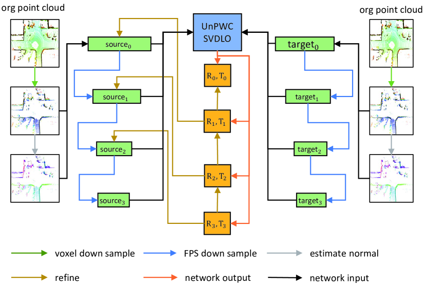
Figure 1: The overall structure of our framework, the original point clouds first voxel down sampling and calculate normal vector of downsampled point clouds, then we obtain multi-level point clouds by multi-level downsample. The high-level point clouds first input the network to calculate the pose, and then the low-level point clouds is refined. The low-level poses are merged with network output poses to obtain the high-level poses.

• We abandon deep learning framework that directly extracts global features from the entire point clouds to fit the pose. Instead, we choose to extract point-level features and output scene flow for each level point. At last, we use SVD decomposition to obtain pose.
  

• We use multi-layer pose estimation. High-level pose is used to refine the lower-level points which make higher level pose has higher accuracy.
  

• We train our network with unsupervised loss and surpass the best existing unsupervised methods on KITTI [5] and Apollo [11], and can even be comparable to the supervised method Lo-Net [7], and are only slightly lower than Lo-Net [7] on Ford [13].

II RELATED WORK

II-A Deep LiDAR Odometry

With the development of computer hardware, deep learning has continued to reduce its operating time, which is sufficient to meet the real-time requirements of lidar odometry. These deep learning methods can be divided into two categories: supervised and unsupervised.
Supervised methods appear relatively early, Velas et al. [21] first map the point clouds s to 2D ”image” by spherical projection and regard pose estimation as a classification problem. Lo-net [7] also use spherical projection and add normal vector which calculated from the surrounding point clouds as network input. Wang et al. [23] adopt a dual-branch architecture to infer 3-D translation and orientation separately instead of a single network. Differently, Li et al. [8] use neural network to calculate the match between points and obtain pose by SVD. Use Pointnet [16] as backbone, Zheng et al. [29] propose a framework for extracting feature from matching keypoint pairs (MKPs) which extracted effectively and efficiently by projecting 3D point clouds s into 2D spherical depth images. PWCLO-Net [22] first introduces the advantages of the scene flow estimation network into the lidar odometry, adds the feature extraction modules in PointPwc [25] to its own network, and introduces the hierarchical embedding mask to remove the points that are not highly matched.
Unsupervised methods appear later. Cho et al. [27] first apply unsupervised approach on deep-learning-based lidar odometry which is an extension of their previous approach [3]. The inspiration of its loss function comes from point-to-plane ICP [10]. Then, Nubert et al. [12] report methods with similarly models, but they use different way to calculate normals and find matching points. In addition, they add plane-to-plane ICP loss. SelfVoxeLO [26] use 3D voxel to downsample and normalize the point clouds, and use 3D convolution network to extract the features of voxel. they also put forward many innovative loss functions to greatly improve the accuracy of pose.

II-B Scene Flow Estimation

Scene flow estimation and lidar odometry are closely related. They also need to find the matching relationship between a pair of points in the point clouds. The purpose of scene flow estimation is to accurately find the changing trend of each point, while lidar odometry is to get the entire point. The change trend between point clouds, but its change trend has only 3-DoF, which is much easier than the change of the 6-DoF of the lidar odometry. These two tasks have their own difficulties, but they can transform each other.
FlowNet3D [9] based on PointNet++, use embeding layers to learn the motion between points in two consecutive frames. PointPWC [25] propose the cost volume method on point clouds and use a muti-level pyramid structure network to estimate muti-level scene flow. Also they first introduce self-supervised losses in sence flow estimate task.

III PROPOSED APPROACH

III-A Problem discription and Data Process

For each timestamp $k\in\mathbb{R}^{+}$, we will get a frame of point cloud $P_{k}$ as input, and the output will be the pose transformation between point clouds $P_{k}$ and $P_{k+1}$. Since we use PointPWC [25] as the backbone network, the KNN points of each point in point clouds are calculated multiple times, if the number of point clouds is too large, We need to spend a lot of time to get results , which cannot meet the real-time requirements of odometry. The point cloud is sorted according to the z-axis first , and the $U\%$ points with the smaller z-axis are removed (roughly remove the ground points, the ground points will also be removed in the preprocessing step in the scene flow estimation task). then we perform voxel downsample on point clouds by dividing the space into equal-sized cells whose side length is $D$ which follows SelfVoxeLO [26]. For each cell, the arithmetic average of all points in it is used to represent it. We name downsampled point cloud as $S_{k}^{0}\in\mathbb{R}^{C_{0}\times 3}$. At last, the normal vector $N_{k}^{0}\in\mathbb{R}^{C_{0}\times 3}$ of $S_{k}^{0}$ is calculated by the plane fitting method [15].

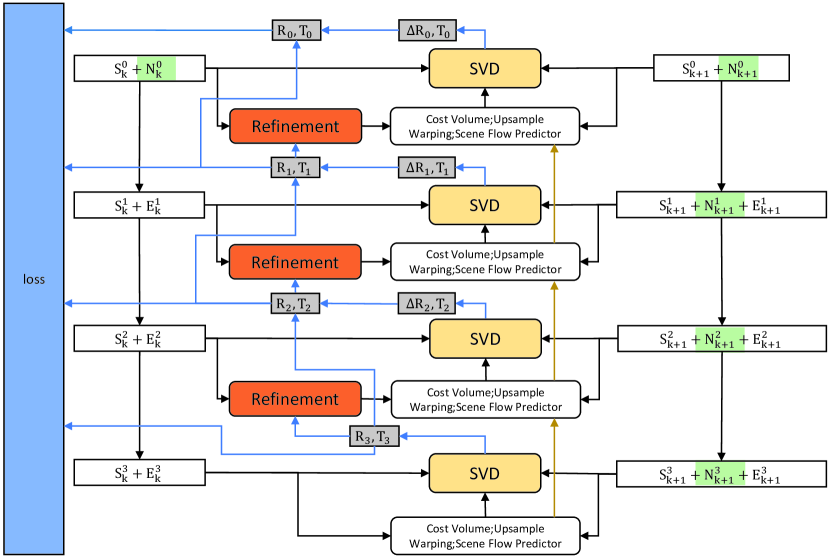
Figure 2: The various modules of our network. Colored modules and data are part of our innovation, and others are originally part in PointPWC [25]. There are 4 levels in total. Level-0 represents the original point cloud and the final output pose. Level-3 is the highest sampled point cloud, and the pose is directly output through SVD without fusion with the higher level.

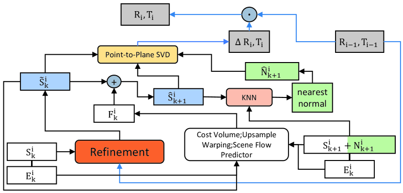
Figure 3: Level-i data processing details.

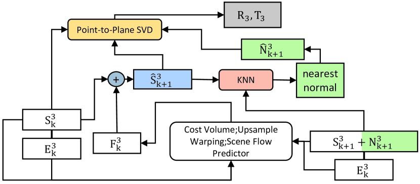
Figure 4: Level-3 data processing details.

III-B Network Architecture

The overall structure of the network is shown in Figure. 2. We first perform multi-level FPS (Farthest Point Sample) and feature extraction on the original point cloud $S_{k}^{0}$, and then start up-sampling and fuse features from the highest Level-3 $S_{k}^{3}$ to estimate the pose of each level.

III-B1 FPS and Feature Extract

We input $S_{k}^{0}$ and $N_{k}^{0}$ into the network, and perform multi-level FPS on $S_{k}^{0}$. $S_{k}^{i+1}$ is FPS from $S_{k}^{i}\in\mathbb{R}^{C_{i}\times 3}$. For each $S_{k}^{i}$, we can get corresponding $N_{k}^{i}\in\mathbb{R}^{C_{i}\times 3}$. While down-sampling, PointConv [24] is used to extract the feature $E_{k}^{i}\in\mathbb{R}^{C_{i}\times M_{i}}$ of $S_{k}^{i}$ which is represented as

$$E_{k}^{i}=\begin{cases}PointConv(N_{k}^{i-1})&i=1\\ PointConv(E_{k}^{i-1})&i>1\\ \end{cases},$$ (1)

so that we can get the multi-level data $(S_{k}^{i},N_{k}^{i},E_{k}^{i})$. Then start from the highest sampling Level-3 ($S_{k}^{3}$ with the least number of points in $S_{k}^{i}$). we perform up-sampling and solve the pose.

III-B2 Up-sampling, Feature Fusion and SVD Sovle the Pose

The detail of this part is shown in Figure. 3 and Figure. 4. Except for the highest level of $S_{k}^{3}$, each level of source point cloud $S_{k}^{i}$ will first be refined by $R_{i+1}\in\mathbb{R}^{3\times 3},T_{i+1}\in\mathbb{R}^{3\times 1}$(we show how to get them later) to obtain $\widetilde{S}_{k}^{i}$ by following formula

$$\widetilde{S}_{k}^{i}=\begin{cases}S_{k}^{i}&i=3\\ R_{i+1}\cdot S_{k}^{i}+T_{i+1}&i<3\\ \end{cases}.$$ (2)

Then we enter source data $(S_{k}^{i},E_{k}^{i})$ and target data $(S_{k+1}^{i},E_{k+1}^{i})$ into feature fusion part of PointPWC [25] (Cost Volume; Upsample; Warping; Scene Flow Predictor) to obtain the scene flow $F_{k}^{i}$. $\widetilde{S}_{k}^{i}$ and $F_{k}^{i}\in\mathbb{R}^{C_{i}\times 3}$ are added as the generated target point cloud $\widehat{S}_{k+1}^{i}$,

$$\widehat{S}_{k+1}^{i}=\widetilde{S}_{k}^{i}+F_{k}^{i}.$$ (3)

By refined source point cloud $\widetilde{S}_{k}^{i}$, generated target point cloud $\widehat{S}_{k+1}^{i}$, target normal vector $N_{k+1}^{i}$, we can obtain the pose $\Delta{R_{i}},\Delta{T_{i}}$ between $\widetilde{S}_{k}^{i}$ and $\widehat{S}_{k+1}^{i}$. Each point in $\widehat{S}_{k+1}^{i}$ finds the nearest neighbor point in $S_{k+1}^{i}$ as the normal vector to obtain $\widehat{N}_{k+1}^{i}$,

$$\begin{split}\widehat{N}_{k+1}^{i}=\{n\in N_{k+1}^{i}|\mathop{\min}\limits_{s}(\widehat{s}-s)^{2},\\ \widehat{s}\in\widehat{S}_{k+1}^{i},s\in S_{k+1}^{i}\}.\end{split}$$ (4)

According to [10], if euler angle of $R$ is closed to zero, we can simplify the formula of point-to-plane ICP and transform it into a standard linear least-squares problem as the following formula

$$\begin{split}\mathop{\min}\limits_{\Delta{R_{i}},\Delta{T_{i}}}&\sum_{j=1}^{K}((\Delta{R_{i}}\cdot\widetilde{s}_{j}+\Delta{T_{i}}-\widehat{s}_{j})\cdot\widehat{n}_{j})\\ &=\mathop{\min}\limits_{x}|A\cdot x-b|^{2}\\ &\widehat{s}_{j}\in\widehat{S}_{k+1}^{i},\widehat{n}_{j}\in\widehat{N}_{k+1}^{i},\widetilde{s}_{j}\in\widetilde{S}_{k}^{i},\\ &A\in\mathbb{R}^{C_{i}\times 6},b\in\mathbb{R}^{C_{i}\times 1},x\in\mathbb{R}^{6\times 1}\end{split}$$ (5)

where

$$b_{j}=\sum_{c}^{x,y,z}\widehat{n}_{j}^{c}\widehat{s}_{j}^{c}-\widehat{n}_{j}^{c}\widetilde{s}_{j}^{c},$$ (6)

$$x=[r^{x},r^{y},r^{z},t^{x},t^{y},t^{z}]^{T}$$ (7)

and

$$\begin{split}A_{j}=&[a_{j}^{x},a_{j}^{y},a_{j}^{z},\widehat{n}_{j}^{x},\widehat{n}_{j}^{y},\widehat{n}_{j}^{z}]\\ &a_{j}^{x}=\widehat{n}_{j}^{z}\widetilde{s}_{j}^{y}-\widehat{n}_{j}^{y}\widetilde{s}_{j}^{z}\\ &a_{j}^{y}=\widehat{n}_{j}^{x}\widetilde{s}_{j}^{z}-\widehat{n}_{j}^{z}\widetilde{s}_{j}^{x}\\ &a_{j}^{z}=\widehat{n}_{j}^{y}\widetilde{s}_{j}^{x}-\widehat{n}_{j}^{x}\widetilde{s}_{j}^{y}\\ \end{split}$$ (8)

which can be solved by using SVD as formula $A=U\Sigma V^{T}$. Next we can get the pseudo-inverse of $A$ as $A^{+}=V\Sigma^{+}U^{T}$. So best result of $x$ can be achieved by

$$x_{opt}=A^{+}b.$$ (9)

At last, We transform $x$ into $\Delta{R_{i}},\Delta{T_{i}}$ by

$$\Delta{T_{i}}=[t^{x},t^{y},t^{z}]$$ (10)

and

$$\begin{split}R^{x}=&\left[\begin{array}[]{ccc}1&0&0\\ 0&\cos r^{x}&-\sin r^{x}\\ 0&\sin r^{x}&\cos r^{x}\end{array}\right]\\ R^{y}=&\left[\begin{array}[]{ccc}\cos r^{y}&0&\sin r^{y}\\ 0&1&0\\ -\sin r^{y}&0&\cos r^{y}\end{array}\right]\\ R^{z}=&\left[\begin{array}[]{ccc}\cos r^{z}&-\sin r^{z}&0\\ \sin r^{z}&\cos r^{z}&0\\ 0&0&1\end{array}\right]\\ &\Delta{R_{i}}=R^{z}\cdot R^{y}\cdot R^{x}.\end{split}$$ (11)

Also we can obtain Level-i final pose $R_{i},T_{i}$ by

$$R_{i}=\begin{cases}\Delta{R_{i}}&i=3\\ \Delta{R_{i}}\cdot R_{i+1}&i<3\\ \end{cases}$$ (12)

and

$$T_{i}=\begin{cases}\Delta{T_{i}}&i=3\\ \Delta{R_{i}}\cdot T_{i+1}+\Delta{T_{i}}&i<3\\ \end{cases}$$ (13)

TABLE I: KITTI odometry evaluation.

	00*		01*		02*		03*		04*		05*		06*		07		08		09		10		Mean on 07-10
Method	$t_{rel}$	$r_{rel}$	$t_{rel}$	$r_{rel}$	$t_{rel}$	$r_{rel}$	$t_{rel}$	$r_{rel}$	$t_{rel}$	$r_{rel}$	$t_{rel}$	$r_{rel}$	$t_{rel}$	$r_{rel}$	$t_{rel}$	$r_{rel}$	$t_{rel}$	$r_{rel}$	$t_{rel}$	$r_{rel}$	$t_{rel}$	$r_{rel}$	$t_{rel}$	$r_{rel}$
ICP-po2po	6.88	2.99	11.21	2.58	8.21	3.39	11.07	5.05	6.64	4.02	3.97	1.93	1.95	1.59	5.17	3.35	10.04	4.93	6.93	2.89	8.91	4.74	7.763	3.978
ICP-po2pl	3.8	1.73	13.53	2.58	9	2.74	2.72	1.63	2.96	2.58	2.29	1.08	1.77	1	1.55	1.42	4.42	2.14	3.95	1.71	6.13	2.6	4.013	1.968
GICP [17]	1.29	0.64	4.39	0.91	2.53	0.77	1.68	1.08	3.76	1.07	1.02	0.54	0.92	0.46	0.64	0.45	1.58	0.75	1.97	0.77	1.31	0.62	1.375	0.648
CLS [20]	2.11	0.95	4.22	1.05	2.29	0.86	1.63	1.09	1.59	0.71	1.98	0.92	0.92	0.46	1.04	0.73	2.14	1.05	1.95	0.92	3.46	1.28	2.148	0.995
LOAM(w/o mapping) [28]	15.99	6.25	3.43	0.93	9.4	3.68	18.18	9.91	9.59	4.57	9.16	4.1	8.91	4.63	10.87	6.76	12.72	5.77	8.1	4.3	12.67	8.79	11.090	6.405
LOAM(w/ mapping) [28]	1.1	0.53	2.79	0.55	1.54	0.55	1.13	0.65	1.45	0.5	0.75	0.38	0.72	0.39	0.69	0.5	1.18	0.44	1.2	0.48	1.51	0.57	1.145	0.498
LO-Net [7]	1.47	0.72	1.36	0.47	1.52	0.71	1.03	0.66	0.51	0.65	1.04	0.69	0.71	0.5	1.7	0.89	2.12	0.77	1.37	0.58	1.8	0.93	1.748	0.793
SelfVoxeLO [26]	NA	NA	NA	NA	NA	NA	NA	NA	NA	NA	NA	NA	NA	NA	3.09	1.81	3.16	1.14	3.01	1.14	3.48	1.11	3.185	1.300
Nubert et al. [12]	NA	NA	NA	NA	NA	NA	NA	NA	NA	NA	NA	NA	NA	NA	NA	NA	NA	NA	6.05	2.15	6.44	3.00	6.245	2.575
Cho et al. [27]	NA	NA	NA	NA	NA	NA	NA	NA	NA	NA	NA	NA	NA	NA	NA	NA	NA	NA	4.87	1.95	5.02	1.83	4.945	1.890
Ours	1.36	0.73	3.39	0.95	1.45	0.60	1.58	0.92	1.09	1.17	1.07	0.55	0.62	0.36	0.71	0.79	1.51	0.75	1.27	0.67	2.05	0.89	1.386	0.775

TABLE II: Ford odometry evaluation.

	ICP-po2po		ICP-po2pl		GICP [17]		CLS [20]		LOAM(w/mapping) [28]		LO-Net [7]		Ours
Seq.	$t_{rel}$	$r_{rel}$	$t_{rel}$	$r_{rel}$	$t_{rel}$	$r_{rel}$	$t_{rel}$	$r_{rel}$	$t_{rel}$	$r_{rel}$	$t_{rel}$	$r_{rel}$	$t_{rel}$	$r_{rel}$
Ford-1	8.2	2.64	3.35	1.65	3.07	1.17	10.54	3.9	1.68	0.54	2.27	0.62	2.99	1.83
Ford-2	16.23	2.84	5.68	1.96	5.11	1.47	14.78	4.6	1.78	0.49	2.18	0.59	3.75	1.38

TABLE III: Apollo odometry evaluation.

ICP-po2po

ICP-po2pl

GICP [17]

NDT-P2D [18]

LOAM(w/mapping) [28]

SelfVoxeLO [26]

Ours

$t_{rel}$

$r_{rel}$

$t_{rel}$

$r_{rel}$

$t_{rel}$

$r_{rel}$

$t_{rel}$

$r_{rel}$

$t_{rel}$

$r_{rel}$

$t_{rel}$

$r_{rel}$

$t_{rel}$

$r_{rel}$

Test mean

22.8

2.35

7.75

1.2

4.55

0.76

57.2

9.4

5.93

0.26

6.42

1.65

4.53

1.30

III-C Loss Function

For unsupervised training, We use the same point cloud down-sampling strategy as [19]. we fisrt use RANSAC [4] to remove the ground points more accurately. Next we also perform voxel downsample. The form of loss is similar to [27], but we only use point-to-plane ICPloss. For the source point cloud $\overline{S}_{k}$, find the closest point in the target point cloud $\overline{S}_{k+1}$ as the matching point. The formula of loss function $L$ is shown as

$$\begin{split}L=&\{\sum_{i=0}^{3}\sum_{\overline{s}_{k}\in\overline{S}_{k}}(R_{i}\cdot\overline{s}_{k}+T_{i}-\overline{s}_{k+1})\cdot\overline{n}_{k+1}|\\ &\mathop{\min}\limits_{\overline{s}_{k+1}}(R_{i}\cdot\overline{s}_{k}+T_{i}-\overline{s}_{k+1})^{2},\\ &\overline{s}_{k+1}\in\overline{S}_{k+1},\overline{n}_{k+1}\in\overline{N}_{k+1}\},\end{split}$$ (14)

where $\overline{N}_{k+1}$ is the normal vector of the target point cloud.

IV EXPERIMENTAL EVALUATION

In this section, we first introduce the implementation details of our total framework and three public datasets we use in experiment. Then, we compare our method with other existing lidar odometry methods to show that our model is competitive. Finally, we perform ablation studies to verify the effectiveness of the innovative part of our model.

IV-A Implementation Details

Our proposed model is implemented in PyTorch [14]. We train it with a single NVIDIA Titan RTX GPU. We optimize the parameters with the Adam optimizer [6] with hyperparameter values of $\beta_{1}=0.9$, $\beta_{2}=0.99$ and $w_{decay}=10^{-5}$. We adopt step scheduler with different stepsizes (20 on KITTI [5] and Ford [13] , 10 on Apollo [11]) and $\gamma=0.5$ to control the training procedure with initial learning rate of $10^{-3}$. The batch size is also different in different datasets(10 on KITTI [5] and Ford [13], 16 on Apollo [11]). During data preprocessing, we drop $U=50\%$ points and side length of voxel cell $D=0.3m$. In order to simplify the training process, we unify the number of voxel cell to $C^{0}=8192$. If the number of points is too small, the existing points will be copied to fill them. If there are too many points, the voxel cells with fewer points will be removed prior. We reserve $C^{1}=2048,C^{2}=512,C^{3}=256$ points for other level of point cloud.

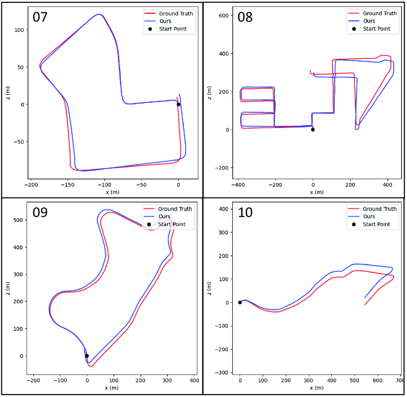
Figure 5: 2D estimated trajectories of our method on sequence 07-10.

IV-B Datasets

IV-B1 KITTI

The KITTI odometry dataset [5] is the most classic data set that most odometry methods will test on it. It has 22 different sequences, only Sequences 00-10 have an official public ground truth. We use sequences 00-06 for training and 07-10 for testing which is the splitting strategy with minimal training data in all other deep learning method.

IV-B2 Ford Campus Vision and Lidar DataSet

Ford [13] only contains two sequences, but there are more moving vehicles than the KITTI dataset which make it more difficult. In order to compare with Lo-net [7], we do not train on it, but use the model trained on KITTI to test directly.

IV-B3 Apollo-SouthBay Dataset

Apollo-SouthBay Dataset [11] collected in the San Francisco Bay area,United States, covers various scenarios. It provides ground truth in all sequences and splits them into traindata, testdata and mapdata three parts. In our experiment, traindata and testdata set are respectively used for train and test which is the same with SelfVoxeLO [26]. It is more complicated and longer than KITTI.

TABLE IV: The ablation study results on KITTI.

	00*		01*		02*		03*		04*		05*		06*		07		08		09		10		Mean on 07-10
Method	$t_{rel}$	$r_{rel}$	$t_{rel}$	$r_{rel}$	$t_{rel}$	$r_{rel}$	$t_{rel}$	$r_{rel}$	$t_{rel}$	$r_{rel}$	$t_{rel}$	$r_{rel}$	$t_{rel}$	$r_{rel}$	$t_{rel}$	$r_{rel}$	$t_{rel}$	$r_{rel}$	$t_{rel}$	$r_{rel}$	$t_{rel}$	$r_{rel}$	$t_{rel}$	$r_{rel}$
MLP	3.67	1.67	4.08	1.11	4.21	1.75	3.08	1.26	2.09	1.48	2.39	1.28	1.57	0.82	17.02	9.38	9.82	4.61	9.82	4.61	22.06	11.53	14.677	7.530
SVD-po2po	1.73	0.80	3.70	1.05	2.25	0.89	2.14	1.22	1.02	0.50	1.24	0.70	0.81	0.49	6.22	4.62	5.11	2.14	9.77	3.57	8.54	4.04	7.410	3.594
SVD-po2pl	1.51	0.78	3.51	0.92	2.06	0.87	2.28	1.12	1.52	1.17	1.09	0.68	0.90	0.63	3.34	1.81	3.14	1.21	3.48	1.53	4.59	1.92	3.639	1.619
Muti-SVD-po2pl w/o refine	1.47	0.77	3.54	0.97	1.75	0.71	2.34	1.11	1.08	0.92	0.98	0.52	0.73	0.37	1.23	1.02	1.91	0.85	2.26	0.96	2.25	1.13	1.911	0.990
Muti-SVD-po2pl w refine	1.35	0.68	3.53	1.00	1.56	0.63	1.47	0.80	0.96	0.90	1.03	0.53	0.67	0.36	1.40	0.77	1.62	0.64	2.00	0.84	1.49	1.11	1.626	0.840

IV-C Evaluation Result

We adopt the official evaluation metrics provide by the KITTI benchmark [5] on all our experiments (include other two datasets). It contains two key indicators: $t_{rel}$ means average translational RMSE (%) on length of 100m-800m and $r_{rel}$ means average rotational RMSE (^∘/100m) on length of 100m-800m. The smaller they are, the better the method is.
We compare our method with the following methods which can be divided into two types. Model-based methods are: ICP-po2po, ICP-po2pl, GICP [17], CLS [20] and LOAM [28]. Learning-based methods are: Lo-Net [7], SelfVoxeLO [26], Nubert et al. [12] and Cho et al. [27]. only Lo-Net is supervised method, others are unsupervised/self-supervised methods.

IV-C1 Evaluation on KITTI

Learning-based methods adopted different splitting strategies for training and testing on KITTI. Nubert et al. and Cho et al. [27] train on sequences 00-08 and test sequences on 09-10. Others train on sequences 00-06 and test sequences on 07-10. Some of they do not show all rsults in their paper and do not release their code, so we use ”NA” represent result we unknow.
Quantitative results are listed in Table. I. As is shown in table, compared with learing-based methods, the results of our method are far better than all current unsupervised methods, even if compared with supervised methods Lo-net [7], we can also even be comparable. Compared with model-based method, we only lose to GISP which with slow calculation speed and the most classic lidar SLAM algorithm LOAM which with the additional mapping step. Fig. 5 plots trajectories in sequences 07-10 of our methods for visualization.

IV-C2 Evaluation on Ford

Quantitative results are listed in Table. II. Both Lo-net [7] and us only train on KITTI and test on Ford. Due to Lo-net [7] is a supervised method, our results are not as good as him, but the gap is not too big. Compared with model-based method, our method only loses to LOAM [28]. In addition, our method surpasses GICP [17] slightly that we inferior to it in KITTI.

IV-C3 Evaluation on Apollo

Apollo-SouthBay dataset [11] is longer and hard than above two dataset, so it can further demonstrate generality of our method. Quantitative results also are listed in Table. III. Not surprisingly, our method can also greatly surpasses the state-of-the-art method with the same training set and test set. Compared with the model-based method, for the first time, we surpassed all methods including LOAM [28] in $t_{rel}$, and lower than LOAM [28]and GICP [17] on $t_{rel}$.

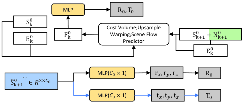
Figure 6: ”MLP” detail structure.

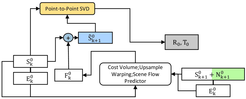
Figure 7: ”SVD po2po” detail structure.

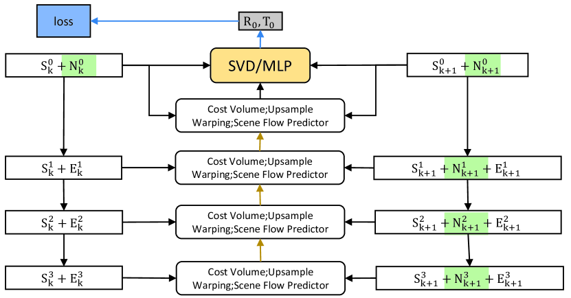
Figure 8: Only use SVD once in Level-0.

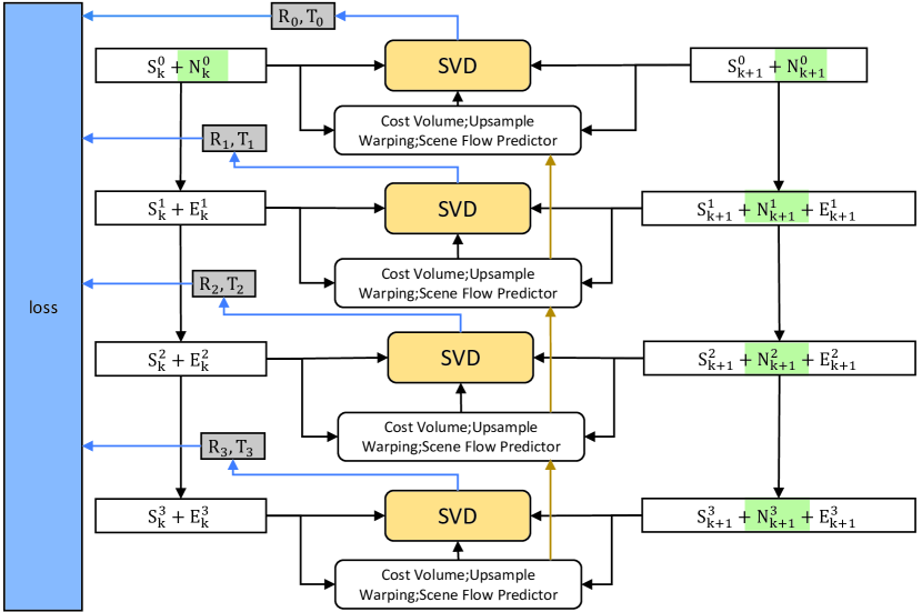
Figure 9: Not refine point clouds.

IV-D Ablation Study

In order to prove the effectiveness of our improvement based on the PointPWC [25], as shown in the Table. IV, we have taken a series of ablation experiments on the KITTI [5]. We test the effect of using different methods to transform the scene flow into pose, and use the simplest method as directly inputing the scene flow into the fully connected layer and output $r^{x,y,z}$ and $t^{x,y,z}$ as benchmarks whose method name is ”MLP” (see Figure. 6). We adopt SVD on point-to-point ICP method [1] which named as ”SVD-po2po” (see Figure. 7), the lidar odometry method DMLO [8] and the point cloud registration method PointDSC [2] use in thier method. Next We adopt SVD on point-to-plane [10] which has been used in our method and we name it as ”SVD-po2pl” (similar to Figure. 4, only the level is different, it is 0 in this part not 3). In the previous experiments, pose is calculated only after the scene flow is obtained at the lowest level, and is not used in the high level. (see Figure. 8). In method ”Muti-SVD-po2pl w/o refine”, SVD is performed in each layer to solve the pose, but the solved pose is not used to improve the low-level point cloud (see Figure. 9). Finally, the method ”Muti-SVD-po2pl w refine” we propose not only obtains the pose of each layer, but also refines low level point cloud. It can be seen that every improvement in our network makes the test results better, which proves that improvement is effective.

V CONCLUSIONS

We proposed a new lidar odometry framework based on the scene flow estimate network PointPWC [25]. Different from other lidar odometry methods, we not only extracted point-level features instead of global-level features, but also use SVD decomposition to convert the scene flow into pose, and additionally use normal vector to convert point-to-point ICP into point-to-plane ICP which further improves the accuracy. We also use high-level pose to improve the low-level point cloud, so that the pose of each layer is associated with each other. The idea of iterative optimization of the pose in the traditional algorithm is integrated into our network. In the future, we will explore the combination of our method and mapping optimization to achieve further breakthroughs.

References

- [1] A. M. Andrew, “Multiple view geometry in computer vision,” Kybernetes, 2001.
- [2] X. Bai, Z. Luo, L. Zhou, H. Chen, L. Li, Z. Hu, H. Fu, and C.-L. Tai, “Pointdsc: Robust point cloud registration using deep spatial consistency,” in CVPR, 2021, pp. 15 859–15 869.
- [3] Y. Cho, G. Kim, and A. Kim, “Deeplo: Geometry-aware deep lidar odometry,” arXiv preprint arXiv:1902.10562, 2019.
- [4] M. A. Fischler and R. C. Bolles, “Random sample consensus: a paradigm for model fitting with applications to image analysis and automated cartography,” Communications of the ACM, vol. 24, no. 6, pp. 381–395, 1981.
- [5] A. Geiger, P. Lenz, and R. Urtasun, “Are we ready for autonomous driving? the kitti vision benchmark suite,” in CVPR. IEEE, 2012, pp. 3354–3361.
- [6] D. P. Kingma and J. Ba, “Adam: A method for stochastic optimization,” in ICLR, 2015.
- [7] Q. Li, S. Chen, C. Wang, X. Li, C. Wen, M. Cheng, and J. Li, “Lo-net: Deep real-time lidar odometry,” in CVPR, 2019, pp. 8473–8482.
- [8] Z. Li and N. Wang, “Dmlo: Deep matching lidar odometry,” in IROS, 2020.
- [9] X. Liu, C. R. Qi, and L. J. Guibas, “Flownet3d: Learning scene flow in 3d point clouds,” in CVPR, 2019, pp. 529–537.
- [10] K.-L. Low, “Linear least-squares optimization for point-to-plane icp surface registration,” Chapel Hill, University of North Carolina, vol. 4, no. 10, pp. 1–3, 2004.
- [11] W. Lu, Y. Zhou, G. Wan, S. Hou, and S. Song, “L3-net: Towards learning based lidar localization for autonomous driving,” in CVPR, 2019, pp. 6389–6398.
- [12] J. Nubert, S. Khattak, and M. Hutter, “Self-supervised learning of lidar odometry for robotic applications,” in ICRA, 2021.
- [13] G. Pandey, J. R. McBride, and R. M. Eustice, “Ford campus vision and lidar data set,” IJRR, vol. 30, no. 13, pp. 1543–1552, 2011.
- [14] A. Paszke, S. Gross, F. Massa, A. Lerer, J. Bradbury, G. Chanan, T. Killeen, Z. Lin, N. Gimelshein, L. Antiga et al., “Pytorch: An imperative style, high-performance deep learning library,” in NIPS, 2019.
- [15] M. Pauly, Point primitives for interactive modeling and processing of 3D geometry. Hartung-Gorre, 2003.
- [16] C. R. Qi, H. Su, K. Mo, and L. J. Guibas, “Pointnet: Deep learning on point sets for 3d classification and segmentation,” in CVPR, 2017, pp. 652–660.
- [17] A. Segal, D. Haehnel, and S. Thrun, “Generalized-icp.” Robotics: science and systems, vol. 2, no. 4, p. 435, 2009.
- [18] T. Stoyanov, M. Magnusson, H. Andreasson, and A. J. Lilienthal, “Fast and accurate scan registration through minimization of the distance between compact 3d ndt representations,” IJRR, vol. 31, no. 12, pp. 1377–1393, 2012.
- [19] Y. Tu and J. Xie, “Undeeplio: Unsupervised deep lidar-inertial odometry,” arXiv preprint arXiv:2109.01533, 2021.
- [20] M. Velas, M. Spanel, and A. Herout, “Collar line segments for fast odometry estimation from velodyne point clouds,” in ICRA. IEEE, 2016, pp. 4486–4495.
- [21] M. Velas, M. Spanel, M. Hradis, and A. Herout, “Cnn for imu assisted odometry estimation using velodyne lidar,” in ICARSC. IEEE, 2018, pp. 71–77.
- [22] G. Wang, X. Wu, Z. Liu, and H. Wang, “Pwclo-net: Deep lidar odometry in 3d point clouds using hierarchical embedding mask optimization,” in CVPR, 2021, pp. 15 910–15 919.
- [23] W. Wang, M. R. U. Saputra, P. Zhao, P. Gusmao, B. Yang, C. Chen, A. Markham, and N. Trigoni, “Deeppco: End-to-end point cloud odometry through deep parallel neural network,” in IROS, 2019.
- [24] W. Wu, Z. Qi, and L. Fuxin, “Pointconv: Deep convolutional networks on 3d point clouds,” in CVPR, 2019, pp. 9621–9630.
- [25] W. Wu, Z. Y. Wang, Z. Li, W. Liu, and L. Fuxin, “Pointpwc-net: Cost volume on point clouds for (self-) supervised scene flow estimation,” in ECCV. Springer, 2020, pp. 88–107.
- [26] Y. Xu, Z. Huang, K.-Y. Lin, X. Zhu, J. Shi, H. Bao, G. Zhang, and H. Li, “Selfvoxelo: Self-supervised lidar odometry with voxel-based deep neural networks,” in CoRL, 2020.
- [27] Younggun, G. Kim, and A. Kim, “Unsupervised geometry-aware deep lidar odometry,” in ICRA. IEEE, 2020, pp. 2145–2152.
- [28] J. Zhang and S. Singh, “Loam: Lidar odometry and mapping in real-time.” Robotics: Science and Systems, vol. 2, no. 9, 2014.
- [29] C. Zheng, Y. Lyu, M. Li, and Z. Zhang, “Lodonet: A deep neural network with 2d keypoint matching for 3d lidar odometry estimation,” in ACM MM, 2020, pp. 2391–2399.