Magneto-structural dependencies in $3d^{2}$ systems : The trigonal bipyramidal V³⁺ complex

Abstract

We introduce a multi-configurational approach to study the magneto-structural correlations in $3d^{2}$ systems. The theoretical framework represents a restricted active space self-consistent field method, with active space optimized to the number of all non-bonding orbitals. To demonstrate the validity and effectiveness of the method, we explore the physical properties of the trigonal bipyramidal spin-one single-ion magnet (C₆F₅)₃trenVCN^tBu. The obtained theoretical results show a good agreement with the experimental data available in the literature. This includes measurements for the magnetization, low-field susceptibility, cw-EPR and photoluminescence spectroscopy. The proposed method may be reliably applied to a variety of $3d^{2}$ magnetic systems. To this end, and for the sake completeness, we provide detailed analytical and numerical representations for the generic Hamiltonian’s effective matrix elements related to the crystal field, exchange, spin-orbit and Zeeman interactions.

I Introduction

Being at the frontier between classical and quantum physics, low-dimensional magnetic systems [1, 2, 3, 4] and molecular magnets [5, 6, 7, 8] continue to generate an ever growing interest among researchers in the field of magnetism for the last few decades. Tailoring the underlying quantum features poses a great challenge for their synthesis, experimental and theoretical characterization. Molecular magnets have great scientific and practical potential. They have been successfully implemented in resonance imaging [9, 10, 11, 12, 13] and stand as a promising candidates for building sensor devices [14, 15, 16] and quantum computing technology [17, 18, 19, 20] to name a few. Despite recent progress [21, 22, 23, 24] engineering the magnetic properties of such systems remains a challenging task and it still requires a lot of efforts to pave the route towards their rationalization and industrial application. Let’s emphasize that the compound’s magnetic behavior is tightly related to the type, number and coordination of ligands with respect to the composing magnetic centers [25, 26, 27]. These has been the subject of extensive interest, here we mention only some prominent and most recent examples, such as the mononuclear $\beta$-diketonate Dy³⁺ single molecular magnet [28], tetranuclear lanthanide metallocene complexes [29], the tetravanadate [V₄O₁₂]^4- anion bridged Cu²⁺ complexes [30] and the single-ion Co²⁺ one [31]. For an overview on the properties of $3d^{2}$ type systems the reader may consult Refs. [32, 33, 34, 35]. Studying the relation between the magnetic properties and the compound’s structure provides a deeper knowledge for the existing zero-field splitting (ZFS) [36, *rudowicz_erratum_1988, 38], quantum character of magnetic anisotropy and all field dependent properties. It further elucidates the driving mechanisms behind the magnetic dynamics that opens up the potential for future applications.

The focus of this study is to reveal the role of the ligand structure in shaping the magnetic and spectroscopic properties of $3d^{2}$ systems and to shed light on the relevant contribution of the crystal field, exchange and spin-orbit interactions. To this end, in complement to the quantum perturbation method, we make use of the variational method [39, 40]. The associated mathematical framework represents a restrictive active space self-consistent field method with an active space spanning all $3d$ orbitals. In order to assess the validity of the proposed multi-configurational approach, we performed a thorough theoretic investigation in the framework of the compound (C₆F₅)₃trenVCN^tBu whose magnetic properties have been experimentally probed [41]. Here, we interpret the experimental data available for the magnetization, low-field susceptibility, cw-EPR spectra and photoluminescence. As the study unfolds, we discuss the role of the crystal field and spin-orbit interactions in the magnetization and susceptibility behavior and the contribution of the exchange interaction to the absorption and emission features.

We would like to emphasize that the proposed approach may be applied to shed light on the magnetic properties of the whole class of $3d^{2}$ systems, regardless of their dimensionality in space – molecular magnets or low-dimensional spin systems. Therefore, we provide analytical results for all interaction terms and effective matrix elements.

The rest of the paper is structured as follows. In Section II, we introduce and elaborate on the theoretical methods used to study the compound under consideration. Further, we introduce some basic notations and give explicit representations of the applied Hamiltonian and all initial basis sates. In Sec. III, we provide details of our computational method that includes representations for all effective matrix elements. Section IV discusses the obtained energy spectrum and its dependence on the action of externally applied magnetic field. A representation of the obtained ZFS in terms of the axial “$D$” and rhombic “$E$” fine structure (FS) parameters is also discussed. Section V covers results on the compound’s magnetic and spectroscopic properties. Finally, a summary of the results is given in Sec. VI. We would like to mention that all numerical results are obtained with the aid of Wofram Mathematica 12.

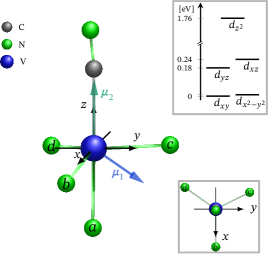
Figure 1: Ball and stick representation of the vanadium ion coordinated by the isocyanide and four nitrogen ligands in the trigonal bipyramidal complex (C₆F₅)₃trenVCN^tBu. The blue, green and gray balls represent the vanadium, nitrogen and carbon elements with coordinates given in Tab. 1. The chemical structure of the compound with included three C₆F₅ rings, is given in Ref. [41]. An illustration of the vector associated to the expectation value of the total magnetic moment $\boldsymbol{\mu}_{n}$, corresponding to the ground state $n=1$ and first excited state $n=2$ in the zero-field case is also shown. The inset in the bottom right shows a view from above the $xy$ plane, while that in top right depicts the respective $d$-orbital energy diagram with normalized energy values, such that the lowest one starts from zero.

Table 1: The values of the azimuthal angle $\varphi$, polar angle $\vartheta$ and radial distance $\varrho$, for each ligand surrounding the vanadium ion residing at the origin of the reference frame, see Fig. 1. All coordinates are calculated with respect to the structural data given in Ref. [41]. The charge number of each ligand and the metal center relative to both $3d$ electrons is given in the penultimate row. The prefactor related to the spin-orbit interactions is given in the last row. Their values are fitted to the magnetization, low-field susceptibility, cw-EPR and Photoluminescence experimental data from Ref. [41].

Lig. Number	$1$	$2$	$3$	$4$	$5$
	C $\backslash$CN$\backslash$	Na	Nb	Nc	Nd	V
$\varphi$ [deg]	$0$	$0$	$0$	$116.42$	$234.74$
$\vartheta$ [deg]	$0$	$177.02$	$96.15$	$97.16$	$100.49$
$\varrho$ [Å]	$2.1566$	$2.1447$	$1.9473$	$1.9577$	$1.9619$
$Z_{i}$	$\backslash 2.365\backslash$	$1.157$	$1.157$	$1.157$	$1.157$	$5.9$
$\kappa$						0.43

II Theoretical background

II.1 General considerations

The magnetic and spectroscopic properties of the compound (C₆F₅)₃trenVCN^tBu are computed and interpreted using a restricted active space self-consistent field approach. The only relativistic contribution accounted for in the calculations is the spin-orbit interaction. In particular, adhering the approximations used in CF theory [42, 43, 44], we describe both unpaired electrons as localized, to a large extent, around the V³⁺ metal center. Accordingly, the constructed optimized reaction space is restricted to the existing $3d^{2}$ configuration. Furthermore, complying to the effective field approach used in the Hartree-Fock method [45, 40, 46], these electrons are exposed to the average field of all remaining “core” electrons that on average do not contribute neither to the splitting nor to the shifting of energy levels in the ensuing energy spectrum. Thus, the considered transition metal complex may be viewed as a good model of a spin-one system consisting of two $3d$ electrons distributed among six effective point-like charges. Those are the vanadium center, the four nitrogen ligands and the isocyanide one. The five ligands reside on the vertices of a distorted trigonal bipyramidal structure (see Fig. 1). We would like to emphasize that in order to overcome the disadvantage of the localized electron approach over the delocalized one used in ligand field theory [44], we introduce five non-variational parameters, one for each ligand, to control the ligands’ electric charge that both $3d$ electrons are exposed to. Moreover, we have one non-variational parameter to address the effect of electrons’ delocalization into the spin-orbit coupling. The resulting six parameters are then allowed to vary in order to achieve better agreement between theory and experimental measurements.

We would like to point out, furthermore, that the contributions of all orbital and spin magnetic-dipole interactions related to both $3d$ unpaired electrons and the constituent nuclei are found negligible and hence omitted from the calculations. Similarly, the hyperfine interactions are also excluded.

Henceforth, we find it convenient to introduce the following notations: $\mathbf{r}_{i}=(\alpha_{i})_{\alpha\in\mathbb{K}}$ designates the $i$-th electron’s position vector, where $\mathbb{K}=\{x,y,z\}$ and $i=1,2$. In spherical coordinates, $\rho_{i}$, $\theta_{i}$ and $\phi_{i}$ are the $i$-th electron’s radial distance, polar and azimuthal angles, respectively. By $\hat{\boldsymbol{\mu}}_{l_{i}}=-\mu_{\mathrm{B}}\hat{\boldsymbol{l}}_{i}$ and $\hat{\boldsymbol{\mu}}_{s_{i}}=-g_{e}\mu_{\mathrm{B}}\hat{\boldsymbol{s}}_{i}$, we denote the corresponding orbital and spin magnetic moment operators, where $\mu_{\mathrm{B}}$ is the Bohr magneton, $g_{e}$ is the electron $g$-factor, $\hat{\boldsymbol{s}}_{i}=(\hat{s}^{\alpha}_{i})_{\alpha\in\mathbb{K}}$ and $\hat{\boldsymbol{l}}_{i}=(\hat{l}^{\alpha}_{i})_{\alpha\in\mathbb{K}}$ are the respective spin and angular momentum operators. The operator of the total magnetic moment $\hat{\boldsymbol{\mu}}$ is given by the sum of total spin $\hat{\boldsymbol{\mu}}_{s}=\hat{\boldsymbol{\mu}}_{s_{1}}+\hat{\boldsymbol{\mu}}_{s_{2}}$ and orbital $\hat{\boldsymbol{\mu}}_{l}=\hat{\boldsymbol{\mu}}_{l_{1}}+\hat{\boldsymbol{\mu}}_{l_{2}}$ ones. The position vector of the $i$-th ligand is denoted by $\mathbf{d}_{i}$ with corresponding spherical coordinates $\varrho_{i}$, $\vartheta_{i}$ and $\varphi_{i}$, where $i=1,\ldots,5$. Here $\vartheta_{i}$ is the polar and $\varphi_{i}$ is the azimuthal angles. Moreover, we set the $z$-axis as the quantization axis and denote the external magnetic field by $\mathbf{B}=(B_{\alpha})_{\alpha\in\mathbb{K}}$ with magnitude $|\mathbf{B}|=B$. In the bra-ket notation, we use $\bar{1}$ instead of $-1$. The electric and magnetic constants are denoted as $\varepsilon$ and $\mu_{o}$, respectively. The Bohr radius is $r_{\mathrm{B}}$. The values of all magnetic moments and their components reported in the text are given in units of Bohr magneton.

II.2 The Hamiltonian

The Hamiltonian of the considered system reads

$$\hat{H}=\hat{U}_{\mathrm{R}}(\mathbf{r}_{1},\mathbf{r}_{2})+\hat{U}_{\mathrm{CF}}(\mathbf{r}_{1},\mathbf{r}_{2})+\hat{U}_{\mathrm{SO}}(\mathbf{r}_{1},\mathbf{r}_{2})+\hat{U}_{\mathrm{Z}}+\hat{H}_{c},$$ (1)

where $\hat{U}_{\mathrm{R}}$ accounts for the Coulomb repulsion between both electrons, $\hat{U}_{\mathrm{CF}}$ represents the interaction of both electrons with the surrounding ligands (crystal field term), $\hat{U}_{\mathrm{SO}}$ is the relativistic term that takes into account the spin-orbital interactions and $\hat{U}_{\mathrm{Z}}$ describes the action of externally applied magnetic field. The last operator $\hat{H}_{c}$ on the right-hand-side in (1) is an invariant of the Hamiltonian system, i.e. $[\hat{H},\hat{H}_{c}]=0$. It produces a constant related to the values of all effective parameters that minimize the energy. It is obtained with respect to the variational function of all bonding and non-bonding “core” electrons. The kinetic terms of both unpaired electrons are also accounted for, since in the case of localized $d$ electrons the relevant expectation values are constants.

In spherical coordinates, the series expansion of the Coulomb term reads [47, 48]

$$\hat{U}_{\mathrm{R}}(\mathbf{r}_{1},\mathbf{r}_{2})\equiv\frac{\gamma}{|\mathbf{r}_{2}-\mathbf{r}_{1}|}=\left\{\begin{array}[]{cc}\displaystyle\gamma\sum_{n=0}^{\infty}\frac{\rho^{n}_{2}}{\rho^{n+1}_{1}}P_{n}(u),&\rho_{1}>\rho_{2},\\[14.22636pt] \displaystyle\gamma\sum_{n=0}^{\infty}\frac{\rho^{n}_{1}}{\rho^{n+1}_{2}}P_{n}(u),&\rho_{2}>\rho_{1},\end{array}\right.$$ (2)

where $\gamma=e^{2}/4\pi\varepsilon$ and for all $n$, $P_{n}(u)$ are the Legendre polynomials, with $u=\sin\theta_{1}\sin\theta_{2}\cos(\phi_{1}-\phi_{2})+\cos\theta_{1}\cos\theta_{2}$.

The total CF operator is given by the sum

$$\hat{U}_{\mathrm{CF}}(\mathbf{r}_{1},\mathbf{r}_{2})=\sum_{j}\big{(}\hat{U}_{j}(\mathbf{r}_{1})+\hat{U}_{j}(\mathbf{r}_{2})\big{)},$$ (3)

where $j$ runs over the number of all ligands. Here, the series expansion of the potential energy accounting for the interaction between the $k$-th ligand and the $i$-th electron is given by [42, 47, 43]

$$\hat{U}_{k}(\mathbf{r}_{i})\equiv\frac{\gamma Z_{k}}{|\mathbf{r}_{i}-\mathbf{d}_{k}|}=\gamma\sum_{n=0}^{\infty}\frac{\rho^{n}_{i}}{\varrho^{n+1}_{k}}P_{n}(v_{i,k}),\quad\varrho_{k}>\rho_{i},\quad\forall i,k,$$ (4)

where, $v_{i,k}=\sin\theta_{i}\sin\vartheta_{k}\cos(\phi_{i}-\varphi_{k})+\cos\theta_{i}\cos\vartheta_{k}$ and $Z_{k}$ is the charge number of the $k$-th ligand to which both $3d$ electrons are exposed. Notice that $Z_{k}$, for all $k$, are fitting parameters that allows one to distinguish between the different ligands. Within the used approximations their values may not be integers, but their lowest value is unity.

The spin-orbit interaction term is given by

$$\hat{U}_{\mathrm{SO}}(\mathbf{r}_{1},\mathbf{r}_{2})\equiv\frac{g_{e}\mu_{o}\mu^{2}_{\mathrm{B}}}{2\pi}\sum_{i}\frac{Z}{\rho^{3}_{i}}\hat{\boldsymbol{l}}_{i}\cdot\hat{\boldsymbol{s}}_{i},\quad i=1,2,$$ (5)

where $Z$ is the charge number of the vanadium metal center with respect to both electrons.

Finally the operator describing the interaction with the externally applied magnetic field reads

$$\hat{U}_{\mathrm{Z}}\equiv-\mu_{\mathrm{B}}\sum_{i}\mathbf{B}\cdot\big{(}\hat{\boldsymbol{l}}_{i}+g_{e}\hat{\boldsymbol{s}}_{i}\big{)},\quad i=1,2.$$ (6)

II.3 Initial basis states

The active space is restricted to the number of all non-bonding orbitals. In other words, we have five $3d$ orbitals and two unpaired electrons. As a result, we end up with forty five quantum basis states, with ten triplets and fifteen singlets. Thus, with respect to the exchange symmetry we get forty states including only active orbitals,

$$\begin{array}[]{l}|\psi_{1,s,m}\rangle\equiv\tfrac{1}{\sqrt{2}}\big{(}|d_{xz},d_{yz}\rangle+(-1)^{s}|d_{yz},d_{xz}\rangle\big{)}|s,m\rangle,\\[5.69046pt] |\psi_{2,s,m}\rangle\equiv\tfrac{1}{\sqrt{2}}\big{(}|d_{xz},d_{xy}\rangle+(-1)^{s}|d_{xy},d_{xz}\rangle\big{)}|s,m\rangle,\\[5.69046pt] |\psi_{3,s,m}\rangle\equiv\tfrac{1}{\sqrt{2}}\big{(}|d_{xz},d_{x^{2}-y^{2}}\rangle+(-1)^{s}|d_{x^{2}-y^{2}},d_{xz}\rangle\big{)}|s,m\rangle,\\[5.69046pt] |\psi_{4,s,m}\rangle\equiv\tfrac{1}{\sqrt{2}}\big{(}|d_{xz},d_{z^{2}}\rangle+(-1)^{s}|d_{z^{2}},d_{xz}\rangle\big{)}|s,m\rangle,\\[5.69046pt] |\psi_{5,s,m}\rangle\equiv\tfrac{1}{\sqrt{2}}\big{(}|d_{yz},d_{xy}\rangle+(-1)^{s}|d_{xy},d_{yz}\rangle\big{)}|s,m\rangle,\\[5.69046pt] |\psi_{6,s,m}\rangle\equiv\tfrac{1}{\sqrt{2}}\big{(}|d_{yz},d_{x^{2}-y^{2}}\rangle+(-1)^{s}|d_{x^{2}-y^{2}},d_{yz}\rangle\big{)}|s,m\rangle,\\[5.69046pt] |\psi_{7,s,m}\rangle\equiv\tfrac{1}{\sqrt{2}}\big{(}|d_{yz},d_{z^{2}}\rangle+(-1)^{s}|d_{z^{2}},d_{yz}\rangle\big{)}|s,m\rangle,\\[5.69046pt] |\psi_{8,s,m}\rangle\equiv\tfrac{1}{\sqrt{2}}\big{(}|d_{xy},d_{x^{2}-y^{2}}\rangle+(-1)^{s}|d_{x^{2}-y^{2}},d_{xy}\rangle\big{)}|s,m\rangle,\\[5.69046pt] |\psi_{9,s,m}\rangle\equiv\tfrac{1}{\sqrt{2}}\big{(}|d_{xy},d_{z^{2}}\rangle+(-1)^{s}|d_{z^{2}},d_{xy}\rangle\big{)}|s,m\rangle,\\[5.69046pt] |\psi_{10,s,m}\rangle\equiv\tfrac{1}{\sqrt{2}}\big{(}|d_{x^{2}-y^{2}},d_{z^{2}}\rangle+(-1)^{s}|d_{z^{2}},d_{x^{2}-y^{2}}\rangle\big{)}|s,m\rangle,\\ \end{array}$$ (7a)

and five core orbital states

$$\begin{array}[]{ll}|\psi_{11,0,0}\rangle\equiv|d_{xz},d_{xz}\rangle|0,0\rangle,&|\psi_{12,0,0}\rangle\equiv|d_{yz},d_{yz}\rangle|0,0\rangle,\\[2.84544pt] |\psi_{13,0,0}\rangle\equiv|d_{xy},d_{xy}\rangle|0,0\rangle,&|\psi_{14,0,0}\rangle\equiv|d_{x^{2}-y^{2}},d_{x^{2}-y^{2}}\rangle|0,0\rangle,\\[2.84544pt] |\psi_{15,0,0}\rangle\equiv|d_{z^{2}},d_{z^{2}}\rangle|0,0\rangle,\end{array}$$ (7b)

where $s=0,1$ and $m=\pm s$ are the total spin and spin-magnetic quantum numbers. Explicit representation of each $d$-state is given in App. A.

III Computational details

III.1 Coulomb terms

Calculating the average values of the Coulomb interaction (2) up to the $4$-th order in the series expansion in the basis (7), we obtain zero off-diagonal matrix elements. For the diagonal ones, with $\langle\psi_{i,s,m}|\hat{U}_{\mathrm{R}}|\psi_{i,s,m}\rangle=E_{i,s,m}$, we have

$$\begin{array}[]{ll}E_{1,s,m}=V_{1}+(-1)^{s}\delta_{1,s}L_{1},&E_{2,s,m}=V_{4}+(-1)^{s}V_{7},\\ E_{3,s,m}=V_{4}+(-1)^{s}V_{7},&E_{4,s,m}=V_{5}+(-1)^{s}V_{8},\\ E_{5,s,m}=V_{4}+(-1)^{s}V_{7},&E_{6,s,m}=V_{4}+(-1)^{s}V_{7},\\ E_{7,s,m}=V_{5}+(-1)^{s}V_{8},&E_{8,s,m}=V_{2}+(-1)^{s}\delta_{1,s}L_{2},\\ E_{9,s,m}=V_{6}+(-1)^{s}V_{9},&E_{10,s,m}=V_{6}+(-1)^{s}V_{9},\\ E_{11,0,0}=V_{1}+\frac{1}{2}L_{1},&E_{12,0,0}=V_{1}+\frac{1}{2}L_{1},\\ E_{13,0,0}=V_{2}+\frac{1}{2}L_{2},&E_{14,0,0}=V_{2}+\frac{1}{2}L_{2},\\ E_{15,0,0}=V_{3},&{}\\ \end{array}$$ (8)

where the explicit representations of $\{V_{i}\}^{9}_{i=1}$ and $\{L_{1},L_{2}\}$, with $Z$ being the only parameter, are provided in App. B. The subscript $m$ shows the $3$-fold degeneracy of the corresponding energy levels.

III.2 CF terms

Within the selected active space, the mixing of states by CF is prominent. In general, we have $\langle\psi_{i,s,m}|\hat{U}_{\mathrm{CF}}|\psi_{j,s^{\prime},m^{\prime}}\rangle=U_{i,s,m;j,s^{\prime},m^{\prime}}$. For the sake of clarity, we denote the respective diagonal elements by $U_{i,s,m}$ to get

$$\begin{array}[]{ll}U_{1,s,m}=U_{xz}+U_{yz},&U_{2,s,m}=U_{xz}+U_{xy},\\ U_{3,s,m}=U_{xz}+U_{x^{2}-y^{2}},&U_{4,s,m}=U_{xz}+U_{z^{2}},\\ U_{5,s,m}=U_{yz}+U_{xy},&U_{6,s,m}=U_{yz}+U_{x^{2}-y^{2}},\\ U_{7,s,m}=U_{yz}+U_{z^{2}},&U_{8,s,m}=U_{xy}+U_{x^{2}-y^{2}},\\ U_{9,s,m}=U_{xy}+U_{z^{2}},&U_{10,s,m}=U_{x^{2}-y^{2}}+U_{z^{2}},\\ U_{11,0,0}=2U_{xz},&U_{12,0,0}=2U_{yz},\\ U_{13,0,0}=2U_{xy},&U_{14,0,0}=2U_{x^{2}-y^{2}},\\ U_{15,0,0}=2U_{z^{2}}.&{}\end{array}$$ (9)

The off-diagonal entries are non-zero for all $s^{\prime}=s$ and $m^{\prime}=m$. Therefore, applying the shorthand notation $U_{i,s,m;j,s,m}\to U_{i,j,s,m}$, we have

$$\begin{array}[]{ll}U_{2,1,s,m}=U_{yz,xy},&U_{3,1,s,m}=U_{yz,x^{2}-y^{2}},\\ U_{4,1,s,m}=U_{yz,z^{2}},&U_{5,1,s,m}=(-1)^{s}U_{xz,xy},\\ U_{6,1,s,m}=(-1)^{s}U_{xz,x^{2}-y^{2}},&U_{7,1,s,m}=(-1)^{s}U_{xz,z^{2}},\\ U_{3,2,s,m}=U_{xy,x^{2}-y^{2}},&U_{4,2,s,m}=U_{xy,z^{2}},\\ U_{5,2,s,m}=U_{xz,yz},&U_{8,2,s,m}=(-1)^{s}U_{xz,x^{2}-y^{2}},\\ U_{9,2,s,m}=(-1)^{s}U_{xz,z^{2}},&U_{4,3,s,m}=U_{x^{2}-y^{2},z^{2}},\\ U_{6,3,s,m}=U_{xz,yz},&U_{8,3,s,m}=U_{xz,xy},\\ U_{10,3,s,m}=(-1)^{s}U_{xz,z^{2}},&U_{7,4,s,m}=U_{xz,yz},\\ U_{9,4,s,m}=U_{xz,xy},&U_{10,4,s,m}=U_{xz,x^{2}-y^{2}},\\ U_{6,5,s,m}=U_{xy,x^{2}-y^{2}},&U_{7,5,s,m}=U_{xy,z^{2}},\\ U_{8,5,s,m}=(-1)^{s}U_{yz,x^{2}-y^{2}},&U_{9,5,s,m}=(-1)^{s}U_{yz,z^{2}},\\ U_{7,6,s,m}=U_{x^{2}-y^{2},z^{2}},&U_{8,6,s,m}=U_{yz,xy},\\ U_{10,6,s,m}=(-1)^{s}U_{yz,z^{2}},&U_{9,7,s,m}=U_{yz,xy},\\ U_{10,7,s,m}=U_{yz,x^{2}-y^{2}},&U_{9,8,s,m}=U_{x^{2}-y^{2},z^{2}},\\ U_{10,8,s,m}=(-1)^{s}U_{xy,z^{2}},&U_{10,9,s,m}=U_{xy,x^{2}-y^{2}}.\\ \end{array}$$ (10a)

Moreover, the average values associated to the singlet only states are given by

$$\begin{array}[]{ll}U_{11,1,0,0}=\sqrt{2}U_{xz,yz},&U_{12,1,0,0}=\sqrt{2}U_{xz,yz},\\ U_{11,2,0,0}=\sqrt{2}U_{xz,xy},&U_{13,2,0,0}=\sqrt{2}U_{xz,xy},\\ U_{11,3,0,0}=\sqrt{2}U_{xz,x^{2}-y^{2}},&U_{14,3,0,0}=\sqrt{2}U_{xz,x^{2}-y^{2}},\\ U_{11,4,0,0}=\sqrt{2}U_{xz,z^{2}},&U_{15,4,0,0}=\sqrt{2}U_{xz,z^{2}},\\ U_{12,5,0,0}=\sqrt{2}U_{yz,xy},&U_{13,5,0,0}=\sqrt{2}U_{yz,xy},\\ U_{12,6,0,0}=\sqrt{2}U_{yz,x^{2}-y^{2}},&U_{14,6,0,0}=\sqrt{2}U_{yz,x^{2}-y^{2}},\\ U_{12,7,0,0}=\sqrt{2}U_{yz,z^{2}},&U_{15,7,0,0}=\sqrt{2}U_{yz,z^{2}},\\ U_{13,8,0,0}=\sqrt{2}U_{xy,x^{2}-y^{2}},&U_{14,8,0,0}=\sqrt{2}U_{xy,x^{2}-y^{2}},\\ U_{13,9,0,0}=\sqrt{2}U_{xy,z^{2}},&U_{15,9,0,0}=\sqrt{2}U_{xy,z^{2}},\\ U_{14,10,0,0}=\sqrt{2}U_{x^{2}-y^{2},z^{2}},&U_{15,10,0,0}=\sqrt{2}U_{x^{2}-y^{2},z^{2}}.\\ \end{array}$$ (10b)

The explicit representation of the functions $U_{\alpha}$ and $U_{\alpha,\beta}$, with $\alpha\neq\beta\in\{xz,yz,xy,x^{2}-y^{2},z^{2}\}$, is shown in App. C. We would like to point out that all functions in (10) are real, with parameters being the ligands’ coordinates, $Z_{1},\ldots,Z_{5}$ and $Z$. The computations are performed up to the forth order in (4).

III.3 Spin-orbit terms

All diagonal matrix elements associated to the total spin-orbit operator (5) are zero. For both electrons, the corresponding spin-orbit coupling $\zeta=\langle g_{e}\mu_{o}\mu^{2}_{\mathrm{B}}Z/2\pi\rho^{3}_{i}\rangle=(35.604\times 10^{-4})Z^{4}$ meV. In order to write down the respective matrix elements in a transparent way, we introduce the parameter $\eta=\kappa\zeta/2\sqrt{2}$, with $0\leq\kappa\leq 1$. The prefactor $\kappa$ is included to accounts for a possible delocalization of both electrons. In other words, if $\kappa\approx 1$, then the initial assumption of localized to a large extent electrons holds. On the other hand, if $\kappa<1$, it would be a sign that the considered electrons may be partially delocalized. Now, for $\langle\psi_{i,s,m}|\hat{U}_{\mathrm{SO}}|\psi_{j,s^{\prime},m^{\prime}}\rangle=Y_{i,s,m;j,s^{\prime},m^{\prime}}$, we get

$$\begin{array}[]{ll}Y_{2,1,\pm 1;1,s,0}=(\pm 1)^{s}\eta,&Y_{3,1,\pm 1;1,s,0}=\pm i(\pm 1)^{s}\eta,\\ Y_{4,1,\pm 1;1,s,0}=\pm i\sqrt{3}(\pm 1)^{s}\eta,&Y_{5,1,\pm 1;1,s,0}=-i(\mp 1)^{s}\eta,\\ Y_{6,1,\pm 1;1,s,0}=(\mp 1)^{s}\eta,&Y_{7,1,\pm 1;1,s,0}=-\sqrt{3}(\mp 1)^{s}\eta,\\ Y_{1,1,\pm 1;2,s,0}=-(\pm 1)^{s}\eta,&Y_{3,1,\pm 1;2,1,\pm 1}=\mp i2\sqrt{2}\eta,\\ Y_{5,1,\pm 1;2,1,\pm 1}=\pm i\sqrt{2}\eta,&Y_{8,1,\pm 1;2,s,0}=(\mp)^{s}\eta,\\ Y_{9,1,\pm 1;2,s,0}=-\sqrt{3}(\mp 1)^{s}\eta,&Y_{1,1,\pm 1;3,s,0}=\mp(\pm 1)^{s}\eta,\\ Y_{6,1,\pm 1;3,1,\pm 1}=\pm i\sqrt{2}\eta,&Y_{8,1,\pm 1;3,s,0}=\pm i(\mp 1)^{s}\eta,\\ Y_{10,1,\pm 1;3,s,0}=-\sqrt{3}(\mp 1)^{s}\eta,&Y_{1,1,\pm 1;4,s,0}=\mp i\sqrt{3}(\pm 1)^{s}\eta,\\ Y_{7,1,\pm 1;4,1,\pm 1}=\pm i\sqrt{2}\eta,&Y_{9,1,\pm 1;4,s,0}=\pm i(\mp 1)^{s}\eta,\\ Y_{10,1,\pm 1;4,1,0}=-(\mp 1)^{s}\eta,&Y_{1,1,\pm 1;5,s,0}=\mp i(\pm 1)^{s}\eta,\\ Y_{6,1,\pm 1;5,1,\pm 1}=\mp i2\sqrt{2}\eta,&Y_{8,1,\pm 1;5,s,0}=\pm i(\mp 1)^{s}\eta,\\ Y_{9,1,\pm 1;5,s,0}=\pm i\sqrt{3}(\mp 1)^{s}\eta,&Y_{1,1,\pm 1;6,s,0}=(\pm 1)^{s}\eta,\\ Y_{8,1,\pm 1;6,s,0}=-(\mp 1)^{s}\eta,&Y_{10,1,\pm 1;6,s,0}=\pm i\sqrt{3}(\mp 1)^{s}\eta\\ \end{array}$$

and

$$\begin{array}[]{ll}\displaystyle Y_{1,1,\pm 1;7,s,0}=-\sqrt{3}(\pm 1)^{s}\eta,&Y_{9,1,\pm 1;7,s,0}=-(\mp 1)^{s}\eta,\\ Y_{10,1,\pm 1;7,s,0}=\mp i(\mp 1)^{s}\eta,&Y_{2,1,\pm 1;8,s,0}=(\pm 1)^{s}\eta,\\ Y_{3,1,\pm 1;8,s,0}=\mp i(\mp 1)^{s}\eta,&Y_{5,1,\pm 1;8,s,0}=\pm i(\pm 1)^{s}\eta,\\ Y_{6,1,\pm 1;8,s,0}=(\mp 1)^{s}\eta,&Y_{2,1,\pm 1;9,s,0}=-\sqrt{3}(\pm 1)^{s}\eta,\\ Y_{4,1,\pm 1;9,s,0}=\mp i(\mp 1)^{s}\eta,&Y_{5,1,\pm 1;9,s,0}=\pm i\sqrt{3}(\pm 1)^{s}\eta,\\ Y_{7,1,\pm 1;9,s,0}=(\mp 1)^{s}\eta,&Y_{10,1,\pm 1;9,1,\pm 1}=\mp i2\sqrt{2}\eta,\\ Y_{3,1,\pm 1;10,s,0}=-\sqrt{3}(\pm 1)^{s}\eta,&Y_{4,1,\pm 1;10,s,0}=(\mp 1)^{s}\eta,\\ Y_{6,1,\pm 1;10,s,0}=\pm i\sqrt{3}(\pm 1)^{s}\eta,&Y_{7,1,\pm 1;10,s,0}=\pm i(\pm 1)^{s}\eta.\\ \end{array}$$

Further, the spin-orbit interactions mix the single orbital states (7b) with the remaining ones, such that

$$\begin{array}[]{lll}Y_{2,1,\pm 1;11,0,0}=\mp i\sqrt{2}\eta,&Y_{3,1,\pm 1;11,0,0}=\sqrt{2}\eta,\\ Y_{4,1,\pm 1;11,0,0}=-\sqrt{6}\eta,&Y_{5,1,\pm 1;12,0,0}=\sqrt{2}\eta,\\ Y_{6,1,\pm 1;12,0,0}=\pm i\sqrt{2}\eta,&Y_{7,1,\pm 1;12,0,0}=\pm i\sqrt{6}\eta,\\ Y_{2,1,\pm 1;13,0,0}=\mp i\sqrt{2}\eta,&Y_{5,1,\pm 1;13,0,0}=\sqrt{2}\eta,\\ Y_{3,1,\pm 1;14,0,0}=\sqrt{2}\eta,&Y_{6,1,\pm 1;14,0,0}=\pm i\sqrt{2}\eta,\\ Y_{4,1,\pm 1;15,0,0}=-\sqrt{6}\eta,&Y_{7,1,\pm 1;15,0,0}=\pm i\sqrt{6}\eta.\\ \end{array}$$

III.4 Zeeman terms

Due to the symmetry of the orbitals in (7), the diagonal matrix elements obtained from (6), $Z_{i,s,m}=\langle\psi_{i,s,m}|\hat{U}_{\mathrm{Z}}|\psi_{i,s,m}\rangle$, depend only on the total spin. Thus, we have $Z_{i,s,m}=g_{e}\mu_{\mathrm{B}}mB_{z}$. Furthermore, since we work in the basis of the spin $z$ component, there are forty spin-only off-diagonal elements corresponding to the mixing between $m=0$ and $m=\pm 1$ states. For all $i=1,\ldots,10$, the non-conjugate ones read $Z_{i,1,\pm 1;i,1,0}=-g_{e}\mu_{\mathrm{B}}(B_{x}\mp iB_{y})/\sqrt{2}$. The remaining off-diagonal elements depend exclusively on the mixing of orbitals. Using the substitution $Z_{i,s,m;j,s,m}\to Z_{i,j,s,m}$, with respect to the states (7a), we obtain

$$\begin{array}[]{ll}Z_{2,1,s,m}=-i\mu_{\mathrm{B}}B_{y},&Z_{3,1,s,m}=-i\mu_{\mathrm{B}}B_{x},\\ Z_{4,1,s,m}=-i\sqrt{3}\mu_{\mathrm{B}}B_{x},&Z_{5,1,s,m}=i(-1)^{s}\mu_{\mathrm{B}}B_{x},\\ Z_{6,1,s,m}=-i(-1)^{s}\mu_{\mathrm{B}}B_{y},&Z_{7,1,s,m}=i(-1)^{s}\sqrt{3}\mu_{\mathrm{B}}B_{y},\\ Z_{3,2,s,m}=i2\mu_{\mathrm{B}}B_{z},&Z_{5,2,s,m}=-i\mu_{\mathrm{B}}B_{z},\\ Z_{8,2,s,m}=-i(-1)^{s}\mu_{\mathrm{B}}B_{y},&Z_{9,2,s,m}=i(-1)^{s}\sqrt{3}\mu_{\mathrm{B}}B_{y},\\ Z_{6,3,s,m}=-i\mu_{\mathrm{B}}B_{z},&Z_{8,3,s,m}=i\mu_{\mathrm{B}}B_{x},\\ Z_{10,3,s,m}=i(-1)^{s}\sqrt{3}\mu_{\mathrm{B}}B_{y},&Z_{7,4,s,m}=-i\mu_{\mathrm{B}}B_{z},\\ Z_{9,4,s,m}=i\mu_{\mathrm{B}}B_{x},&Z_{10,4,s,m}=-i\mu_{\mathrm{B}}B_{y},\\ Z_{6,5,s,m}=i2\mu_{\mathrm{B}}B_{z},&Z_{8,5,s,m}=-i(-1)^{s}\mu_{\mathrm{B}}B_{x},\\ Z_{9,5,s,m}=-i(-1)^{s}\sqrt{3}\mu_{\mathrm{B}}B_{x},&Z_{8,6,s,m}=-i\mu_{\mathrm{B}}B_{y},\\ Z_{10,6,s,m}=-i(-1)^{s}\sqrt{3}\mu_{\mathrm{B}}B_{x},&Z_{9,7,s,m}=-i\mu_{\mathrm{B}}B_{y},\\ Z_{10,7,s,m}=-i\mu_{\mathrm{B}}B_{x},&Z_{10,9,s,m}=i2\mu_{\mathrm{B}}B_{z}\\ \end{array}$$

and with the consideration of singlet states (7b), we get

$$\begin{array}[]{ll}Z_{11,1,0,0}=i\sqrt{2}\mu_{\mathrm{B}}B_{z},&Z_{12,1,0,0}=-i\sqrt{2}\mu_{\mathrm{B}}B_{z},\\ Z_{11,2,0,0}=-i\sqrt{2}\mu_{\mathrm{B}}B_{x},&Z_{13,2,0,0}=i\sqrt{2}\mu_{\mathrm{B}}B_{x},\\ Z_{11,3,0,0}=i\sqrt{2}\mu_{\mathrm{B}}B_{y},&Z_{14,3,0,0}=-i\sqrt{2}\mu_{\mathrm{B}}B_{y},\\ Z_{11,4,0,0}=-i\sqrt{6}\mu_{\mathrm{B}}B_{y},&Z_{15,4,0,0}=i\sqrt{6}\mu_{\mathrm{B}}B_{y},\\ Z_{12,5,0,0}=i\sqrt{2}\mu_{\mathrm{B}}B_{y},&Z_{13,5,0,0}=-i\sqrt{2}\mu_{\mathrm{B}}B_{y},\\ Z_{12,6,0,0}=i\sqrt{2}\mu_{\mathrm{B}}B_{x},&Z_{14,6,0,0}=-i\sqrt{2}\mu_{\mathrm{B}}B_{x},\\ Z_{12,7,0,0}=i\sqrt{6}\mu_{\mathrm{B}}B_{x},&Z_{15,7,0,0}=-i\sqrt{6}\mu_{\mathrm{B}}B_{x},\\ Z_{13,8,0,0}=-i2\sqrt{2}\mu_{\mathrm{B}}B_{z},&Z_{14,8,0,0}=i2\sqrt{2}\mu_{\mathrm{B}}B_{z}.\\ \end{array}$$

IV Energy spectrum

IV.1 Zero-field spectrum

The energy spectrum of the considered vanadium complex is obtained after direct diagonalization of the total matrix given by the sum of the four matrices corresponding to the interactions in Hamiltonian (1) and with elements given in Sec. III. The spectrum is non-degenerate and hence it is build up of forty five energy levels for both cases $B=0$ and $B\neq 0$. Since the value of the ground state energy does not affect the final splitting and shifting of levels, the respective eigenvalues are normalized such that the ground state energy equals zero. The resulting energy level sequence depends on two sets of parameters. On one hand we have the ligands’ coordinates given in Tab. 1 and on the other the fitting parameters $\kappa$, $Z$ and $Z_{k}$, for $k=1,\ldots,5$. The relevant structural parameters are experimentally determined and provided in Ref. [41]. The values of all “$Z$” parameters are given in the penultimate row of Tab. 1 and in conjunction with $\kappa=0.43$ their values are fitted in accordance to the low-field susceptibility, magnetization, cw-EPR experimental and Photoluminescence data from Ref. [41].

The energy spectrum in the absence of an external magnetic field is shown on Fig. 2 (a). The value of each energy level is provided in App. D. Fig. 2 (b) depicts the first three energy levels, which represent the obtained ZFS [49, 50, 51, 52, 38] and its dependence on $\kappa$.

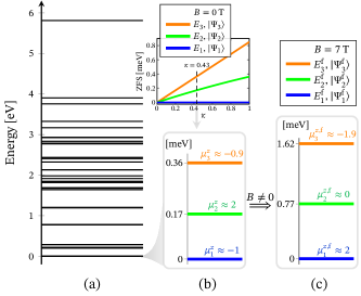
Figure 2: Energy spectrum of the complex (C₆F₅)₃trenVCN^tBu. The energy levels are shifted such that the ground state one is zero. (a) Represents all energy spectra consisting of forty five levels. (b) Depicts the first three energy levels governing the compound’s magnetic properties in the zero-field case with parameters given in Tab. 1. It further shows the splitting of these levels as a function $\kappa$. (c) Shows the shifting of the first three levels under the action of an externally applied magnetic field along the $z$ axis of the compounds reference frame, see Fig. 1, with magnitude $B\equiv B_{z}=7$ T. The blue, green and orange lines indicate the ground, first and second excited energy levels, respectively. The corresponding expectation values of the $z$-component of the total magnetic moment in [$\mu_{\mathrm{B}}$] are also given. The respective designations in the case of absence and presence of magnetic field are $\mu^{z}_{n}$ and $\mu^{z,\mathrm{f}}_{n}$, $n=1,2,3$. The superscript “f” marks the selected magnetic field direction and magnitude.

The combined effect of spin-orbital interactions and distorted trigonal bipyramidal geometry, see Fig. 1, determines the ground state as a mixing involving only $m=0$ and $m=-1$ spin states, i.e.

$$|\Psi_{1}\rangle= (-0.14+0.14i)|\psi_{1,1,0}\rangle-(0.14+0.15i)|\psi_{1,1,\bar{1}}\rangle$$

$$+(0.25-0.24i)|\psi_{2,1,0}\rangle+(0.25+0.27i)|\psi_{2,1,\bar{1}}\rangle$$

$$-(0.13-0.13i)|\psi_{3,1,0}\rangle-(0.13+0.14i)|\psi_{3,1,\bar{1}}\rangle$$

$$-(0.24-0.23i)|\psi_{5,1,0}\rangle-(0.25+0.25i)|\psi_{5,1,\bar{1}}\rangle$$

$$+(0.29-0.28i)|\psi_{6,1,0}\rangle+(0.29+0.31i)|\psi_{6,1,\bar{1}}\rangle$$

$$-(0.065-0.063i)|\psi_{8,1,0}\rangle-(0.066+0.071i)|\psi_{8,1,\bar{1}}\rangle$$

$$+\sum_{n\geq 2}O\big{(}10^{-n}\big{)}|\psi_{\ldots}\rangle.$$ (11)

Therefore, we have a probability of approximately $47\%$ to observe the system in $m=0$ state and $53\%$ in a state with $m=-1$. Consequently, with expectation values given in Bohr magneton units, for the total magnetic moment we have $\boldsymbol{\mu}_{1}=(-0.0171,1.4091,-1.0865)$. The orbital contribution is negligible, thus $\boldsymbol{\mu}_{s,1}=(-0.0181,1.4103,-1.0612)$ and $\boldsymbol{\mu}_{l,1}=(0.001,-0.0011,-0.0253)$.

The distortion in coordination geometry also determines the first excited state as a superposition of only $m=1$ spin states

$$|\Psi_{2}\rangle= (0.19-0.21i)|\psi_{1,1,1}\rangle-(0.34-0.37i)|\psi_{2,1,1}\rangle$$

$$+(0.17-0.20i)|\psi_{3,1,1}\rangle+(0.33-0.35i)|\psi_{5,1,1}\rangle$$

$$-(0.39-0.44i)|\psi_{6,1,1}\rangle+(0.089-0.098i)|\psi_{8,1,1}\rangle$$

$$+\sum_{n\geq 2}O\big{(}10^{-n}\big{)}|\psi_{\ldots}\rangle,$$ (12)

where $\boldsymbol{\mu}_{2}=(0.0157,0.0037,2.0509)$ and $\boldsymbol{\mu}_{s,2}=(0,0,1.9994)$. Thus, any excitation to $E_{2}$ would be associated to an almost fully polarized magnetic moment. An illustration of both vectors $\boldsymbol{\mu}_{1}$ and $\boldsymbol{\mu}_{2}$ is shown on Fig. 1.

The second excited state, $|\Psi_{3}\rangle$, is given by the same superposition of initial basis states as the ground state (IV.1), but with different probability coefficients values, see (D). The corresponding total magnetic moment is $\boldsymbol{\mu}_{3}=(0.0036,-1.4241,-0.9634)$, with contribution from the spin component $\boldsymbol{\mu}_{s,3}=(0.0182,-1.4105,-0.9379)$.

It is essential to emphasize that the first almost total singlet state, with approximately $99\%$ probability to observe $s=0$, is

$$|\Psi_{26}\rangle= 0.092|\psi_{11,0,0}\rangle-0.24|\psi_{12,0,0}\rangle-0.34|\psi_{13,0,0}\rangle$$

$$+0.18|\psi_{14,0,0}\rangle-0.26|\psi_{2,0,0}\rangle+0.31|\psi_{3,0,0}\rangle$$

$$+0.74|\psi_{5,0,0}\rangle-0.11|\psi_{6,0,0}\rangle-0.23|\psi_{8,0,0}\rangle$$

$$+\sum_{n\geq 2}O\big{(}10^{-n}\big{)}|\psi_{\ldots}\rangle.$$ (13)

The corresponding energy level lies very high in the zero-temperature energy spectrum shown on Fig. 2 (a). It is approximately $1.846$ eV. Such a large exchange coupling is typical for transition metal complexes with localized around the metal center electrons and suggests a possible phosphorescence observation. On the other hand, the small energy gaps $\Delta E_{21}\approx 0.17$ meV and $\Delta E_{31}\approx 0.36$ meV, make the zero-field and low-field magnetic properties of the considered complex highly sensitive to the variations in temperature. This feature is clearly demonstrated by the temperature dependence of the susceptibility depicted on Fig. 3 and the magnetization behavior shown on Fig. 4 at $B=1$ T. This point will be discussed below in Sec. V.

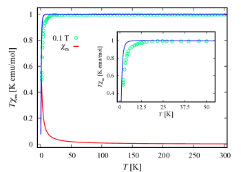
Figure 3: Molar susceptibility of (C₆F₅)₃trenVCN^tBu multiplied by the temperature as a function of the temperature. The experimental data, taken from Ref. [41], are depicted by green circles. The computational results are represented by a solid blue line. For the sake of completeness the calculated low-field molar susceptibility is shown by a solid red line. All relevant parameters are given in Tab. 1.

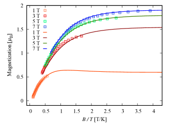
Figure 4: Magnetization plot of the compound (C₆F₅)₃trenVCN^tBu at $1$, $3$, $5$ and $7$ T magnetic field values. The experimental data provided by Ref. [41] are depicted by empty squares. The solid curves represent the theoretical results discussed in Sec. V. The values of all corresponding parameters are given in Tabs. 1 and 2.

Table 2: Magnetization ($4$-th row) for given magnetic field values $B$ and temperatures to the saturation values ($1$-st row). The last row indicates the variation of the effective angle “$\nu$” between the vectors of the applied magnetic field and the magnetization with the change of $B$. For comparison, the third row shows the $z$ component of the molecule’s magnetic moment at the same temperature and magnetic field values, where in this case $\nu$ represents the angle between the magnetic field and $z$ axis of the compound’s reference frame.

$T$ [K]	$\leq 0.1$	$0.2$	$0.6$	$1$	$1.35$
$B$ [T]	$0$	$1$	$3$	$5$	$7$
$m_{z}$ [$\mu_{\mathrm{B}}$]	$-1.0865$	$-0.4666$	$1.3382$	$1.7712$	$1.9240$
$M$ [$\mu_{\mathrm{B}}$]	$0$	$0.5952$	$1.5434$	$1.7920$	$1.9046$
$\nu$ [deg]		$47.4681$	$34.8129$	$24.6142$	$16.9022$

According to all approximations taken into account in Sec. II.1, the obtained ZFS results due to the spin-orbit interactions acting within the CF basis. Therefore, any consideration with $\kappa\to 0$ leads a 3-fold degenerate ground state. For further details see Fig. 2 (b). On the other hand, for $\kappa\to 1$ the ZFS increases to the extent that the theory is no longer able to reproduce the overall experimental observations. To gain insight into the interrelationship between the two physically different notions: ZFS and CF, we recommend the interested reader to consult Refs. [36, *rudowicz_erratum_1988, 38].

IV.2 The magnetic field effect

The interaction of the considered complex with the externally applied magnetic field is taken into account by the Zeeman effective matrix with elements given in Sec. III.4. The zero-field spectrum is not degenerate with respect to $m$, due to the distorted geometry, and so no Zeeman splitting can be observed. As a consequence, we witness only shifting of the energy levels. However, the change of the ground state takes place in a way that resembles the Zeeman effect.

An example of how the energy levels shift under the action of the externally applied magnetic field, for $B_{z}\equiv B=7$ T, is demonstrated on Fig. 2 (c). The superscript “f” indicates the selected magnetic field direction and the magnitude. The resulting shifting is related to a change of the eigenstates. The second excited state from the zero-field spectrum (IV.1) is now the ground state. Thus, we have $|\Psi_{2}\rangle\to|\Psi^{\mathrm{f}}_{1}\rangle$, where the variation in the probability coefficients value is negligible, such that $\boldsymbol{\mu}_{2}\to\boldsymbol{\mu}^{\mathrm{f}}_{1}=(0.015,0.0048,2.0288)$. This is not the case with the first excited state $|\Psi^{\mathrm{f}}_{2}\rangle$, which is a transformation of the zero-field ground state (IV.1). We get

$$|\Psi^{\mathrm{f}}_{2}\rangle= (0.18-0.21i)|\psi_{1,1,0}\rangle+(0.048+0.043i)|\psi_{1,1,\bar{1}}\rangle$$

$$-(0.32-0.37i)|\psi_{2,1,0}\rangle-(0.081+0.074i)|\psi_{2,1,\bar{1}}\rangle$$

$$+(0.17-0.19i)|\psi_{3,1,0}\rangle+(0.040+0.039i)|\psi_{3,1,\bar{1}}\rangle$$

$$+(0.31-0.36i)|\psi_{5,1,0}\rangle+(0.081+0.069i)|\psi_{5,1,\bar{1}}\rangle$$

$$-(0.38-0.43i)|\psi_{6,1,0}\rangle-(0.096+0.086i)|\psi_{6,1,\bar{1}}\rangle$$

$$+(0.084-0.098i)|\psi_{8,1,0}\rangle+(0.022+0.020i)|\psi_{8,1,\bar{1}}\rangle$$

$$+\sum_{n\geq 2}O\big{(}10^{-n}\big{)}|\psi_{\ldots}\rangle.$$ (14)

Hence, the orbital and spin terms given in Sec. III.4 enhance the probability of observing the $m=0$ state from $47\%$ at $B=0$ T to approximately $95\%$ in the considered case. At the same time the value of corresponding energy level increases and $E_{1}\to E^{\mathrm{f}}_{2}$. Respectively, the expectation values of the total magnetic moment also change. We get $\boldsymbol{\mu}_{1}\to\boldsymbol{\mu}^{\mathrm{f}}_{2}=(0.0022,0.6102,-0.1193)$.

The second excited state $|\Psi^{\mathrm{f}}_{3}\rangle$ is a transformation of $|\Psi_{3}\rangle$, and it favors the $m=-1$ outcome with approximately $94.8\%$ probability rather than $46.4\%$ obtained for the zero-field case. As a result, we get $\boldsymbol{\mu}_{3}\to\boldsymbol{\mu}^{\mathrm{f}}_{3}=(0.0011,-0.6053,-1.9755)$. For the explicit representation of the second excited quantum state, see e.g. (D).

We would like to point out that the observed shifting of energy levels and the absence of a genuine Zeeman splitting in the present study is similar to the same feature found for the magnetic behavior of Ni₄Mo₁₂ molecular magnet [53] and Er³⁺ complexes [54], except that for the latter compounds such a dependence of the fine structure on an externally applied magnetic field is more complex and it is tightly related to the exchange interactions [55].

IV.3 Orbital-energy diagram

In addition to the energy spectrum we introduce the splitting of the $3d$ orbitals. The corresponding diagram is depicted on the top right in Fig. 1. Each single electron $3d_{\alpha}$ orbital has an energy $U_{\alpha}$ given in App. C, where $\alpha\in\{xz,yz,xy,x^{2}-y^{2},z^{2}\}$. As expected, due to the presence of CN ligand the $d_{z^{2}}$ orbital is the highest in energy. For the same reason $d_{xz}$ and $d_{yz}$ orbitals are higher in energy than the $d_{xy}$ and $d_{x^{2}-y^{2}}$ ones, which is opposite to the case of identical ligands.

Each eigenstate can be schematically represented as a superposition of such diagrams with included spin-configurations. For example, the first excited state given in (IV.1) is the superposition of six spin-orbital configurations shown on Fig. 5. The approximate probability of observing each one is given in percentage.

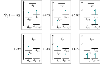
Figure 5: Sketch representing the first excited state in the zero-field energy spectrum as a superposition of spin-orbital diagrams. The corresponding energy scale is depicted on Fig. 1. The diagrams’ arrangement is given in accordance to the superposition of the configuration state functions (IV.1), with only the first six states included. The coefficients are replaced by the corresponding probabilities, given in percentages. The individual spins with their mutual orientations are illustrated as green half-arrows.

IV.4 The determination of the ZFS parameters $D$ and $E$

Since we have neglected all dipole-dipole magnetic interactions the obtained FS shown on Figs. 2 (b) is entirely determined from the spin-orbit interactions within CF basis states (7). Thus, quantifying the ZFS in terms of the corresponding parameters resulting from the quantum perturbational approach and related algebraic representations (see e.g. [36, *rudowicz_erratum_1988] and references therein), we need only the spin Hamiltonian

$$\hat{\mathcal{H}}=\hat{\mathbf{S}}\cdot\mathbf{D}\cdot\hat{\mathbf{S}},$$ (15)

where $\hat{\mathbf{S}}=(\hat{S}_{\alpha})_{\alpha\in\mathbb{K}}$ is the effective spin-one operator of the considered system, $\mathbf{D}$ is a symmetric tensor, with elements $D_{\alpha\beta}\in\mathbb{R}$, $\alpha,\beta\in\mathbb{K}$. Hereafter, we will see that a direct mapping between the spectrum of (15) and those depicted on Fig. 2 (b) is not feasible.

With respect to the applied method, the FS relevant to the low-lying energy levels is quantified by the energy gaps $\Delta E_{21}=0.1708$, $\Delta E_{31}=0.3649$ and $\Delta E_{32}=0.1941$ meV. The associated functions are the ground state (IV.1), first (IV.1) and second (D) excited states. Represented only within the effective spin space they read $|\Psi_{1}\rangle\to C(|0\rangle-|\bar{1}\rangle)$, $|\Psi_{2}\rangle\to|1\rangle$ and $|\Psi_{3}\rangle\to C(|0\rangle+|\bar{1}\rangle)$, respectively, where $C=$$1/\sqrt{2}$. Here, the superposition of the ground and second excited states cannot be addressed by the spin Hamiltonian (15) since in our case the CF contributes significantly to the mixing of states. As a consequence, we could perform a sort of mapping and extract useful information for the elements of $\mathbf{D}$ only by rising the complex’s symmetry to $C_{3v}$ and preserving the overall ZFS that equals $0.3649$ meV. Now, calculating the energy level sequence and associated eigenstates in the case of ideal trigonal bipyramidal geometry, we have $D_{\alpha\beta}=0$ for all $\alpha\neq\beta$, $D_{yy}=D_{xx}=\Delta E_{31}/3$ and $D_{zz}=-2\Delta E_{31}/3$ meV. Owing to the relation between ZFS parameters $(D,E)$ and the tensor elements [49, 56], we get $D=-\Delta E_{31}$ and $E=0$.

In contrast to the positive value of $D$ obtained in Ref. [41] and hence $|0\rangle$ spin-one ground state, our calculations suggests the opposite scenario. In other words, the ground state energy level should be $2$-fold degenerate and represented by the $|1\rangle$, $|\bar{1}\rangle$ states, with $D\approx-2.943$ cm^-1 and $|0\rangle$ being the excited state.

V Magnetic and spectroscopic properties

V.1 Magnetization and susceptibility

The obtained FS in the zero-field energy spectrum shown on Fig. 2 (b), with energy gaps smaller than half of a meV, clearly indicates that the compound’s magnetic moment

$$\mathbf{m}(T)=\varOmega^{-1}\sum^{45}_{n=1}\boldsymbol{\mu}_{n}e^{-E_{n}/k_{B}T},\ \text{with}\ \ \varOmega=\sum_{n=1}^{45}e^{-E_{n}/k_{B}T},$$ (16)

rapidly decreases by magnitude with increasing temperature. The dependance on $\kappa$ and therefore on the overall ZFS, is shown on Fig. 7 (a), where $0\leq\kappa\leq 1$. Thus, for $\kappa\leq 0.1$ the effect of temperature is most prominent in the domain $0.1$ to $1$ K. On the contrary, when the ZFS is large, or $\kappa=1$, in the same temperature domain the magnitude of $\mathbf{m}$ remains almost unchanged. Moreover, as it is depicted on Fig. 6 (a), $\mathbf{m}$ also deviates from its initial direction when $T\to 0$.

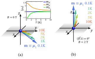
Figure 6: Evolution of the effective magnetic moment (16) in the temperature domain $0.1\leq T\leq 10$ K. The blue ball represents the vanadium ion residing at the center of the local reference frame with orientation depicted on Fig. 1. (a) Shows the temperature dependence in the absence of an external magnetic field. (b) Depicts the case of an applied along the $z$ axis magnetic field, with magnitude $B=2$ T.

Even at low magnetic field values, the small ZFS renders the magnetic behavior of the considered complex very susceptible to temperature variations, see Fig. 7 (b). An exception is the domain $0\leq\kappa\leq 0.086$ for $T\leq 0.1$ K, where the contribution of the externally applied magnetic field to the mixing of the ground state is greater than the spin-orbit one. Hence, the smaller the ZFS the greater the population [57] of first two excited states for a given temperature. As an example, for $\kappa=0.43$, $T=10$ K and $B=0.1$ T the population rates of the first two excited energy levels are almost equal. In particular, we have the probability to observe $40\%$ of the constituents in the powder sample at the ground state, $p_{2}\approx 33.5\%$ in the first excited state and $p_{3}\approx 26.2\%$ in the third one. As a result, we obtain a prompt decrease in the low-field susceptibility in the temperature domain $0<T\leq 10$ K. A comparison between theory and experiment is depicted on Fig. 3, where the fraction between the corresponding molar mass and density is found to be approximately $0.975$ [cm³/mol].

Since the zero-field spectrum is non-degenerate the action of the externally applied magnetic field changes the FS of the energy spectrum by only increasing the corresponding energy gaps, see for example Fig. 2 (c). The eigenstates also change, such that their magnetic sequence resembles the spin Zeeman splitting. Thus, while reaching saturation of the magnetization, the probability of observing a fully polarized magnetic moment, along the magnetic field direction, at the ground state equals unity.

With magnetization data collected on a powder sample the magnetization $\mathbf{M}(B,T)$ is computed as an arithmetic mean of the magnetic moments $\mathbf{m}$ of all complexes that can be represented as a parity transformation one to another regarding their local reference frame shown on Fig. 1. The temperature dependence of magnetization per complex, $M=|\mathbf{M}(T)|$, for some external magnetic field values is depicted on Fig. 4. The consistency with the experimental data from Ref. [41] is obtained for values of the model parameters in Tab. 1 and the angle $\nu$ between $\mathbf{M}(B,T)$ and $\mathbf{B}$ in the bottom row of Tab. 2.

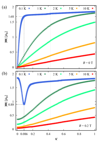
Figure 7: The magnitude of magnetic moment (16) as a function of reduction coefficient $\kappa$ at selected temperatures. The dashed gray line shows the value of $\kappa$ obtained from the comparison with the experimental data from Ref. [41] and given in Tab. 1. (a) Shows the $\kappa$ dependence in the absence of the external magnetic field. (b) Depicts the low-field case, with $B\equiv B_{z}=0.2$ T. The dashed black line indicates the minimum of $|\mathbf{m}|$ at $T=0.1$ K due to the interplay between Zeeman and spin-orbit interactions.

At $7$ T and $T\leq 1$ K the magnetization is approximately $0.963$ times its maximal value reached at about $B=10$ T. In the case of low field values the obtained small reduction of the magnetization at $B=1$ T and $T\leq 0.8$ K, shown on Fig. 4, is due to the presence of single-ion anisotropy, see the energy barriers depicted on Figs. 8 and 9. As an example, taking $B=1$ T and $T=0.8$ K, for the magnetization of a powder sample we have $M=0.6413$. Yet calculating the magnetic moment (16), for $\{\widehat{\mathbf{B}\ \pm x},\widehat{\mathbf{B}\ \pm y},\widehat{\mathbf{B}\ z}\}=$ $\{58.53^{\circ},58.53^{\circ},47.46^{\circ}\}$, we get $\mathbf{m}_{+}=(0.582,1.455,-0.215)$ and $\mathbf{m}_{-}=(-0.739,0.195,0.466)$. Hence, the energy required to fully polarize a single molecule strongly depends on the direction of the externally applied magnetic field in the compound’s reference frame. In order to shed more light on the existing single-ion anisotropy, we explore how the complex’s energy depends on the direction angles $\{a,b,c\}$ [57, 49, 47] of the magnetic moment (16) taken with respect to the reference frame shown on Fig. 1. Since the $z$ axis coincides with the principle axis of the ideal trigonal geometry case and we do not have a $\bot C_{2}$ axis of symmetry, we set $\{a,b,c\}=\{\widehat{\mathbf{m}\ x},\widehat{\mathbf{m}\ y},\widehat{\mathbf{m}\ z}\}$. Moreover, in view of the fact that at $T=0.1$ K the ground state is about a hundred percent populated, excited energy levels have a negligible contribution to the obtained energy barrier profile. Therefore, we obtain a small energy barrier with height $E_{br}\approx\Delta E_{21}/3$ meV, shown on the insets in Fig. 8 and 9. The barrier separates two different states of equal population in the case $T=0.1$ K, one of which is the ground state (IV.1) indicated by a green circle. The representation of the second state, shown by a red circle, depends on the axis along which the magnetic moment $\mathbf{m}$ reverses. For example, considering the $z$ axis, with barrier depicted on Fig. 8 (a), we find that the second state is (IV.1). The evolution of the energy barrier with respect to $B$ is depicted on the background in Figs. 8 and 9. The value of $E_{br}$ depends on the direction of the applied magnetic field. Taking the $z$ axis, for example, with $\mathbf{B}=(0,0,B_{z})$, we get $E_{br}\approx\Delta E_{21}/3$ meV. On the other hand, for $\mathbf{B}=(0,0,-B_{z})$ the barrier’s height is approximately $1.6$ meV. The most prominent value of $E_{br}$ is obtained in the case $\mathbf{B}=(0,-B_{y},0)$, reaching nearly $2$ meV. The energy barrier rapidly vanishes by increasing the temperature. The corresponding dependence is shown on Fig. 10 (a) and is intrinsically related to the evolution of $\mathbf{m}$ depicted on Fig. 6 (a). Moreover, Fig. 9 shows that the barrier’s height reduces significantly by decreasing the value of $\kappa$, demonstrating how it depends on the ZFS sketched on Fig. 2 (b). Note that as expected no energy barrier is observed along the $x$ axis, by virtue of the temperature dependence of $m_{x}$ shown on Fig. 6 (a).

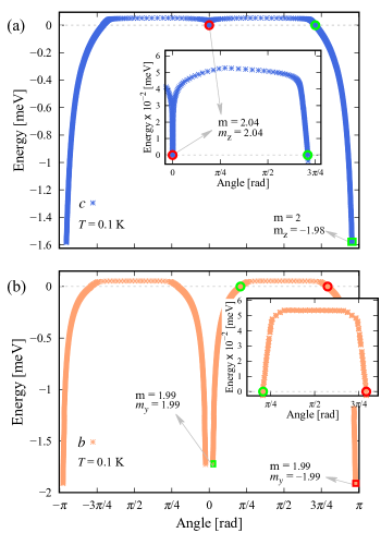
Figure 8: Ground state energy of a single molecule as a function of the direction angles of the magnetic moment (16) at $T=0.1$ K and parameters given in Tab. 1. The energy is normalized with respect to its minimum at $B=0$, indicated by a green circle and with magnetic moment components shown on Fig. 6 (a). The second energy minimum that could be equally occupied is indicated by a red circle. Both insets show the energy barrier profile and its center between the two zero-field minima. The minimal energy to both fully polarized states $m_{\alpha}\to\pm 2$, with $\alpha=z,y$, is indicated by squares. (a) depicts the dependence on the angle “$c$” between $\mathbf{m}$ and the $z$ axis of the compounds reference frame, see Fig. 1, and (b) shows the ground state energy as a function of the angle “$b$” between $\mathbf{m}$ and the $y$ axis of the compounds reference frame. Notice that no energy barrier is observed along the $x$ axis.

V.2 cw-EPR

According to the cw-EPR experimental observations reported in Ref. [41] the Vanadium based complex responds to a $240$ GHz microwave radiation at approximately $3.75$, $6.55$ and $10.4$ T magnetic field values and $T=8$ K. Since all three transitions are related to a spin triplet states the selection rules are $\Delta s=0$ and $|\Delta m|=1,2$. We would like to point out that these transitions are selected for the sake of convenience and for mixed states the associated selection rules should be interpreted in accordance with Refs. [49, 58]. The corresponding excitations, with energy approximately $0.992$ meV, are reasonably well reproduced by the present theoretical approach. They are related to the existing anisotropy that determines the $y$ component of the magnetic moment (16) as a dominant transverse component in the whole temperature range, see Fig. 6 (a) and the energy barriers depicted on Fig. 8. In other words, with respect to the compounds reference frame illustrated on Fig. 1, the resonance condition is satisfied only when the magnetic field vector lies in the $(zy)$ plane and forms a certain angle with the $z$ and $y$ axes. Thus, only certain units in the powder sample with the appropriate orientation with respect to the direction of $\mathbf{B}$ will be magnetically excited, contributing on average to the change in magnetization from the perspective of laboratory reference frame.

By taking $\mathbf{B}=B\mathbf{n}$, where $\mathbf{n}=(n_{\alpha})_{\alpha\in\mathbb{K}}$ is the field’s unit vector with respect to the compound’s reference frame, we obtain that the resonance occurs for $n_{x}=0$, $0.4212\leq n_{y}\leq 0.4338$ and $-0.901\leq n_{z}\leq-0.907$.

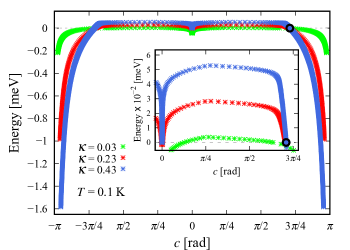
Figure 9: The ground state energy of a single molecule as a function of the direction angle “$c$” between $\mathbf{m}$ and the $z$ axis of the compounds reference frame and its dependence on the reduction parameter $\kappa$ to the spin-orbit coupling. No angle dependence is observed at $\kappa=0$. The energy is normalized to the value obtained in the case $B=0$, indicated with a black circle. For additional details see Fig. 8 (a). The inset depicts detailed view of the energy barrier profile.

The first transition at $3.75$ T refers to a magnetic excitation with $|\Delta m|=2$. It involves the ground and the second excited states. The population rate at the ground state is $62.5\%$ and represented by a superposition of the three spin-one triplets with coefficients given in percentage, it reads $|\Psi^{3.75}_{1}\rangle\to 0.1\%|1,1\rangle+23.8\%|1,0\rangle+76.1\%|1,\bar{1}\rangle$. Respectively, for the second excited state, we get $|\Psi^{3.75}_{3}\rangle\to 81.3\%|1,1\rangle+16.3\%|1,0\rangle+2.4\%|1,\bar{1}\rangle$.

The second excitation at $6.55$ T is associated to a transition between the ground and the first excited states, with $|\Delta m|=1$. The calculated population of the ground state is about $75.2\%$, which explains the higher intensity of the relevant peak compared to that of the first excitation. With respect to the probabilities distribution among the three spin triplets, both states read $|\Psi^{6.55}_{1}\rangle\to 1.7\%|1,1\rangle+18.9\%|1,0\rangle+80.4\%|1,\bar{1}\rangle$ and $|\Psi^{6.55}_{2}\rangle\to 13.2\%|1,1\rangle+68.4\%|1,0\rangle+18.4\%|1,\bar{1}\rangle$.

The third peak at approximately $10.4$ T is associated to a transition between the first and second excited states that can be represented as $|\Psi^{10.4}_{2}\rangle\to 11.9\%|1,1\rangle+72.4\%|1,0\rangle+15.7\%|1,\bar{1}\rangle$ and $|\Psi^{10.4}_{3}\rangle\to 88.5\%|1,1\rangle+11\%|1,0\rangle+0.5\%|1,\bar{1}\rangle$, respectively. The corresponding selection rule is $|\Delta m|=1$. The population of the first excited level at $8$ K is about $10.1\%$ which is consistent with the observed low intensity of the peak [41].

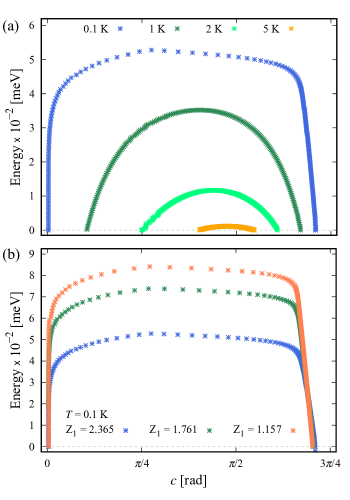
Figure 10: (a) Temperature dependence of the energy barrier calculated with respect to the $z$ axis. The excited states contribute for $T>0.1$ K. More details are shown on the inset in Fig. 8 (a). Subfigure (b) depicts how the barrier’s height along the $z$ axis changes with respect to the cyanide charge number $Z_{1}$ at $T=0.1$ K.

V.3 Photoluminescence

The photoluminescence spectroscopy performed on (C₆F₅)₃trenVCN^tBu in 2-methyltetrahydrofuran at $77$ K, reported in Ref. [41], shows a continuous near-infrared emission with spectral peak at approximately $1.240$ $\mu$m in the excitation wavelength range $550-750$ nm. According to the $s=1$ ground state, the transitions to all photo-excitations are triplet-singlet related. Respectively, the observed phosphorescence is associated to a singlet-triplet relaxation process. Furthermore, the large difference between the excitation and emission energies suggests that the overall relaxation pathway may incorporate transitions with different vibronic modes. To this end, in an attempt to reproduce the photoluminescence data, we simulate variations in the polar and azimuthal angles for all ligands with a value no larger than $0.63^{\circ}$, since within the domain $(-0.63^{\circ},0.63^{\circ})$ the ZFS depicted on Fig. 2 (b) remains invariant. This simulation allows us to trace the corresponding change of the electronic energy levels and the extent of spin-multiplet mixing in the resulting eigenstates. Actually, the phonon energies and interactions are not considered. Moreover, for brevity variations in the radial position of the ligands are not computed.

For $\Delta\vartheta_{i}=0^{\circ}$ and $\Delta\varphi_{i}=0^{\circ}$, $i=1,\ldots,5$, the function (IV.1) is the first singlet state with energy $E_{26}=1.84694$ eV, see App. D. At this point the group of eigenstates $\{|\Psi_{23}\rangle,|\Psi_{24}\rangle,|\Psi_{25}\rangle\}$ are all $s=1$ states with more than $99.9\%$ probability. For example

$$|\Psi_{23}\rangle= 0.55i|\psi_{10,1,0}\rangle-0.38|\psi_{10,1,\bar{1}}\rangle-0.38|\psi_{10,1,1}\rangle$$

$$\!+0.45i|\psi_{9,1,0}\rangle-0.31|\psi_{9,1,\bar{1}}\rangle-0.31|\psi_{9,1,1}\rangle$$

$$-0.08i|\psi_{7,1,0}\rangle+0.055|\psi_{7,1,\bar{1}}\rangle+0.055|\psi_{7,1,1}\rangle$$

$$+0.048i|\psi_{4,1,0}\rangle-0.033|\psi_{4,1,\bar{1}}\rangle-0.033|\psi_{4,1,1}\rangle$$

$$+\sum_{n\geq 2}O\big{(}10^{-n}\big{)}|\psi_{\ldots}\rangle.$$

In this case, the lower possible excitation wavelength lies in the experimentally observed domain and is approximately $671$ nm. However, the only spin-allowed emission near to the observed one, with no intersystem crossing, is of low probability and related to the transition $|\Psi_{26}\rangle\to|\Psi_{15}\rangle$. It is about $1.16$ $\mu$m, where

$$|\Psi_{15}\rangle= (-0.61-0.27i)|\psi_{1,1,0}\rangle+(0.26-0.6i)|\psi_{1,1,\bar{1}}\rangle$$

$$-(0.17+0.08i)|\psi_{2,1,0}\rangle+(0.07-0.17i)|\psi_{2,1,\bar{1}}\rangle$$

$$+(0.039+0.018i)|\psi_{5,1,0}\rangle-(0.017-0.039i)|\psi_{5,1,\bar{1}}\rangle$$

$$-(0.1+0.044i)|\psi_{6,1,0}\rangle+(0.042-0.099i)|\psi_{6,1,\bar{1}}\rangle$$

$$+(0.113+0.051i)|\psi_{8,1,0}\rangle-(0.048-0.112i)|\psi_{8,1,\bar{1}}\rangle$$

$$+\sum_{n\geq 2}O\big{(}10^{-n}\big{)}|\psi_{\ldots}\rangle.$$ (17)

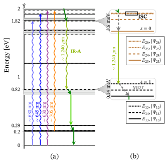
Figure 11: (a) Energy level diagram of (C₆F₅)₃trenVCN^tBu up to $2$ eV with possible absorption bands and relaxation pathway reproducing the photoluminescence and UV–Vis–NIR spectroscopy measurments reported in Ref. [41]. For all $i=1,\ldots,5$ the black lines represent the case with $\Delta\vartheta_{i}=0^{\circ}$, $\Delta\varphi_{i}=0^{\circ}$ shown on Fig 2 (a). The gray solid fields depict bands of energy levels associated to a possible continuous or discrete variations in the angular positions of all ligands, in the intervals $-0.63^{\circ}\leq\Delta\vartheta_{i}\leq 0.63^{\circ}$, $-0.63^{\circ}\leq\Delta\varphi_{i}\leq 0.63^{\circ}$. The blue, violet and orange arrows refer to spin-allowed ground and excited state transitions, respectively, where $\Delta\vartheta_{i}=0.585^{\circ}$, $\Delta\varphi_{i}=0^{\circ}$. Accordingly, the olive green arrow depicts singlet-triplet radiative decay at $1240$ nm related to the observed emission, see Ref. [41]. Non-radiative decays are illustrated by solid non-curved arrows. The light-green arrow shows a transition at about $3$ $\mu$m. (b) A magnification shows the FS for the case $\Delta\vartheta_{i}=0.585^{\circ}$, $\Delta\varphi_{i}=0^{\circ}$, with possible intersystem crossing (ISC) and magnetic dipole transitions (MDT) depicted by dashed gray arrow.

A better theoretical description of the photoluminescence spectroscopy is obtained by varying the polar and azimuthal angles of all ligands with an amount of $\pm 0.63^{\circ}$ to their initial values given in Tab. 1. The resulting emission wavelengths take values in the range $1.230-1.250$ $\mu$m. A particular case with $\Delta\vartheta_{i}=0.585^{\circ}$ and $\Delta\varphi_{i}=0^{\circ}$ for all $i=1,\ldots,5$ is depicted on Fig. 11 (a). The most considerable is the shifting related to the observed emission involving the set of energy levels $\{E_{13},E_{14},E_{15}\}$. An absorption band and a possible relaxation pathway are depicted by curved arrows, where the absorption at $705$ nm is of very low probability rate for $T<300$ K. The corresponding radiative decay at about $1240$ nm is a singlet-triplet transition. In particular, the compound undergoes a transition from $|\Psi^{\Delta}_{23}\rangle$ to $|\Psi^{\Delta}_{15}\rangle$, where the former state is now the $99.5\%$ singlet

$$|\Psi^{\Delta}_{23}\rangle= -0.11|\psi_{1,0,0}\rangle+0.25|\psi_{2,0,0}\rangle-0.2|\psi_{3,0,0}\rangle$$

$$-0.73|\psi_{5,0,0}\rangle-0.016|\psi_{6,0,0}\rangle-0.031|\psi_{7,0,0}\rangle$$

$$+0.25|\psi_{8,0,0}\rangle+0.045|\psi_{9,0,0}\rangle-0.051|\psi_{11,0,0}\rangle$$

$$+0.26|\psi_{12,0,0}\rangle+0.38|\psi_{13,0,0}\rangle-0.13|\psi_{14,0,0}\rangle$$

$$+\sum_{n\geq 1}O\big{(}10^{-n}\big{)}|\psi_{\mathrm{trip}.}\rangle.$$

The superposition in the energy eigenstate $|\Psi^{\Delta}_{15}\rangle$ has almost the same expression as (V.3). For more details see App E. In addition, Fig. 11 (b) depicts the FS of this transition. Depending on the values of $\Delta\vartheta_{i}$ and $\Delta\varphi_{i}$, the calculations predict a different extent of intersystem crossing between two group of levels related to the states $\{|\Psi^{\Delta}_{23}\rangle,|\Psi^{\Delta}_{24}\rangle,|\Psi^{\Delta}_{25}\rangle\}$ and $\{|\Psi^{\Delta}_{26}\rangle,|\Psi^{\Delta}_{27}\rangle,|\Psi^{\Delta}_{28}\rangle\}$. The relaxation to the ground state after the emission involves only spin triplet states and is assumed to be related to vibrational modes.

In spite of the fact that the proposed approach sheds light on the experimentally observed phosphorescence, the decay corresponding to a wavelength of nearly $3\mu$m remains unresolved (see Fig. 11 (a)).

We would like to point out that the isocyanide member may allow significant stretching of its bond to the vanadium center, as it is discussed in Ref. [41]. In this respect, variations equal or less than $\pm 0.05$ Å in the corresponding radial position has no significant contribution to the energy spectrum shown on Fig. 11 (a). Yet, any value closer to $\pm 0.1$ Å considerably increases the shifting of the energy levels and leads to a different ZFS.

VI Summary

To gain useful insight into the magneto-structural dependencies in $3d^{2}$ systems and the mutual influence of crystal field, exchange and spin-orbit interactions on their magnetic behavior, we performed an extensive and detailed theoretical investigation of the magnetic and spectroscopic properties of the compound (C₆F₅)₃trenVCN^tBu. Using a multi-configurational method with active space restricted to all five $d$ orbitals, we reproduce and interpret the available in literature experimental data [41]. This includes calculations for the magnetization, low-field susceptibility, cw-EPR and photoluminescence spectroscopy. For more details see e.g. Sec. V.

In general, in the parameterization scheme associated to the proposed method there are three sets of non-variational parameters. The first set includes the coordinates of all ligands, obtained from the structural analysis. The second comprises of the charge numbers of all ligands and metal centers, see Sec. II.2, in particular (4). Moreover, the second set accounts for a control parameter to the spin-orbit coupling, denoted in the present study by $\kappa$ and discussed at the beginning of Sec. III.3. Finally, the third contains the components of the unit vector associated to the applied magnetic field, taken with respect to the compound’s reference frame (see e.g. Fig. 1). It further includes all derived quantities, such as the effective angle given in Tab. 2. Let us stress that these parameters uniquely characterize the compound under consideration.

In particular, the study of (C₆F₅)₃trenVCN^tBu points out that the electrons are partially delocalized. This may be traced back to the lower than expected values of the prefactor $\kappa$ and charge number $Z$ of the vanadium ion, see Tab. 1. This is also evident from the larger than expected value of $Z_{1}$. Furthermore, the calculations show that the difference between the values of the charge number of nitrogen and isocyanide ligands plays a significant role in shaping the low-field low-temperature magnetic properties. Accordingly, there is an optimal range for this difference where one obtains good agreement with the available experimental data. For example, reducing the value of $Z_{1}$ from Tab. 1 results in a better agreement with the low-susceptibility measurements and in a worse reproduction of the low-field magnetization, cw-EPR and photoluminescence data. This is due to the corresponding decreasing in energy of the $d_{xz}$ and $d_{yz}$ orbitals and increasing of ZFS. However, the value of $Z_{1}$ does not contribute considerably to the zero-field ground state magnetic properties. In particular, setting $Z_{1}=Z_{i}$, for all $i=2,\ldots,5$, with $Z_{i}$ given in Tab. 1, the orientation of the total magnetic moment at the ground state slightly changes from $\boldsymbol{\mu}_{1}=(-0.0171,1.4091,-1.0865)$ to $\boldsymbol{\mu}_{1}=(-0.02695,1.36805,-1.01942)$ (see Fig. 6 (a) and Sec. IV.1). As a result, for $T\to 0$ the magnitude and orientation of $\mathbf{m}$ given in (16) slightly change. The $d_{xz}$, $d_{yz}$ orbitals are now lower in energy than the $d_{xy}$, $d_{x^{2}-y^{2}}$ ones and the ZFS is stronger. We have $\Delta E_{21}=0.2855$, $\Delta E_{31}=0.5785$ and $\Delta E_{32}=0.2929$ meV. Consequently, the population of the corresponding levels changes leading to a different temperature dependence of the magnetic moment (16) in the case $T>0$. Furthermore, the anisotropy energy [45, 57, 59, 60] also changes, such that the corresponding energy barrier’s height increases. An example is depicted on Fig. 10 (b), where for $T=0.1$ K and $Z_{1}=1.157$ with respect to the $z$ axis we have $E_{br}\approx 0.084$ meV.

Let us stress that in the case of ideal trigonal bipyramidal geometry we obtain an energy level sequence that can be directly related to the conventional ZFS Hamiltonian [36, *rudowicz_erratum_1988, 61]. Thus, one has the case of $2$-fold degenerate ground state and an excited state related to $m=0$ spin state, with $D<0$ and $E\to 0$. Nevertheless, the proposed multi-configurational scheme still gives the energy eigenstates as a linear combination of different configuration functions. The comparison with the axial $D$ and rhombic $E$ ZFS parameters is provided in Sec. IV.4.

An essential feature observed in the presence of external magnetic field is the evolution of FS. The shifting of energy levels due to the action of $\mathbf{B}$ is discussed in Sec. IV.2. Nevertheless, another example of how the Zeeman and spin-orbit terms interfere causing this effect is evident from the dependence of magnetic moment (16) on the reduction coefficient $\kappa$. This effect is prominent for low-temperatures and is demonstrated on Fig. 7 (b). Within the studied low symmetry complex, there exist a minimum value of $|\mathbf{m}|$ that corresponds to a maximal degeneracy of the ground state energy level in the case $B\neq 0$. With respect to the case depicted on Fig. 7 (b), for $\kappa=0.086$ and $B\equiv B_{z}=0.2$ T, the ground state level is $2$-fold degenerate. As a result, the magnitude of $\mathbf{m}$ drops below its zero-field value, shown on Fig. 7 (a), marking the crossing point of the competition between Zeeman and spin-orbit terms.

Within the considered localized electron approach the exchange interactions do not contribute to the ground state magnetic properties of the studied compound. Generally, this is true for all $3d^{2}$ compounds since the corresponding energy gaps are larger than $1$ eV. For example, the first singlet state in the energy spectrum shown on Fig. 2 is approximately $1.846$ eV, see equation (IV.1). Therefore, the only exchange related magnetic transitions occur due to absorption or emission.

This study provides analytical and numerical results for the expectation values of all possible interaction terms, energy eigenstates and the related magnetic moments. In general, the used method and the ensuing analytical expressions can be directly applied to all $3d^{2}$ single molecular magnets and low-dimensional systems. Some candidates, for example, are those consisting of Ti²⁺, Cr⁴⁺ and Mn⁵⁺ metal centers.

Appendix A State representation

The single electron $3d$ states (7) are given by the product between the radial wavefunction $R_{32}(\rho)$, the spherical harmonics $Y^{m_{l}}_{2}(\theta,\phi)$ [47, 62] and the spin states $|m_{s}\rangle$, where $m_{l}=0,\pm 1,\pm 2$ and $m_{s}=\pm 1/2$. For example, $|d_{z^{2}}\rangle|m_{s}\rangle\to R_{32}(\rho)Y^{0}_{2}|m_{s}\rangle$. Omitting the spin term, we have

$$\begin{array}[]{l}|d_{xz}\rangle\to R_{32}(\rho)\frac{1}{\sqrt{2}}\big{(}Y^{-1}_{2}(\theta,\phi)-Y^{1}_{2}(\theta,\phi)\big{)},\\[4.26773pt] |d_{yz}\rangle\to R_{32}(\rho)\frac{i}{\sqrt{2}}\big{(}Y^{1}_{2}(\theta,\phi)+Y^{-1}_{2}(\theta,\phi)\big{)},\\[4.26773pt] |d_{xy}\rangle\to R_{32}(\rho)\frac{i}{\sqrt{2}}\big{(}Y^{-2}_{2}(\theta,\phi)-Y^{2}_{2}(\theta,\phi)\big{)},\\[4.26773pt] |d_{x^{2}-y^{2}}\rangle\to R_{32}(\rho)\frac{1}{\sqrt{2}}\big{(}Y^{2}_{2}(\theta,\phi)+Y^{-2}_{2}(\theta,\phi)\big{)}.\\ \end{array}$$

Appendix B Exchange integrals

The exchange integrals $\{V_{i}\}^{9}_{i=1}$ and $\{L_{1},L_{2}\}$ in (8) read

$$\begin{array}[]{lll}V_{1}=\frac{42601}{483840}\frac{\gamma}{r_{\mathrm{B}}}Z,&V_{2}=\frac{43459}{483840}\frac{\gamma}{r_{\mathrm{B}}}Z,&V_{3}=\frac{29731}{322560}\frac{\gamma}{r_{\mathrm{B}}}Z,\\[4.26773pt] V_{4}=\frac{81211}{967680}\frac{\gamma}{r_{\mathrm{B}}}Z,&V_{5}=\frac{27833}{322560}\frac{\gamma}{r_{\mathrm{B}}}Z,&V_{6}=\frac{26689}{322560}\frac{\gamma}{r_{\mathrm{B}}}Z,\\[4.26773pt] V_{7}=\frac{5707}{967680}\frac{\gamma}{r_{\mathrm{B}}}Z,&V_{8}=\frac{949}{322560}\frac{\gamma}{r_{\mathrm{B}}}Z,&V_{9}=\frac{169}{35840}\frac{\gamma}{r_{\mathrm{B}}}Z,\\[4.26773pt] L_{1}=\frac{3991}{483840}\frac{\gamma}{r_{\mathrm{B}}}Z,&L_{2}=\frac{65}{13824}\frac{\gamma}{r_{\mathrm{B}}}Z.&{}\end{array}$$

Appendix C CF integrals

The functions $U_{\alpha}$ and $U_{\alpha,\beta}$, with $\alpha\in\{xz,yz,xy,x^{2}-y^{2},z^{2}\}$, are the sum of five terms $U^{(i)}_{\alpha}$ and $U^{(i)}_{\alpha,\beta}$, respectively, where $i=1,\ldots,5$. For example, $U_{yz}=\sum^{5}_{i=1}U^{(i)}_{yz}$.

For all $i$, the functions that enter into the diagonal elements read

$$U^{(i)}_{xz}= \tfrac{\gamma Z_{i}}{32\varrho^{5}_{i}Z^{4}}\Big{(}-21870r_{\mathrm{B}}^{4}+144\varrho_{i}^{2}r_{\mathrm{B}}^{2}Z^{2}+32\varrho_{i}^{4}Z^{4}+54r_{\mathrm{B}}^{2}$$

$$\times\!(675r_{\mathrm{B}}^{2}+8\varrho_{i}^{2}Z^{2})\cos[2\varphi_{i}]-42525r_{\mathrm{B}}^{4}\!\cos[2(\varphi_{i}\!-\!2\vartheta_{i})]$$

$$+24300r_{\mathrm{B}}^{4}\!\cos[2(\varphi_{i}\!-\vartheta_{i})]-216\varrho_{i}^{2}r_{\mathrm{B}}^{2}Z^{2}\!\cos[2(\varphi_{i}\!-\vartheta_{i})]$$

$$-48600r_{\mathrm{B}}^{4}\cos[2\vartheta_{i}]+432\varrho_{i}^{2}r_{\mathrm{B}}^{2}Z^{2}\cos[2\vartheta_{i}]-85050r_{\mathrm{B}}^{4}$$

$$\times\cos[4\vartheta_{i}]+24300r_{\mathrm{B}}^{4}\cos[2(\varphi_{i}+\vartheta_{i})]-216\varrho_{i}^{2}r_{\mathrm{B}}^{2}Z^{2}$$

$$\times\cos[2(\varphi_{i}+\vartheta_{i})]-42525r_{\mathrm{B}}^{4}\cos[2(\varphi_{i}+2\vartheta_{i})]\Big{)},$$

$$U^{(i)}_{yz}= \tfrac{\gamma Z_{i}}{32\varrho^{5}_{i}Z^{4}}\Big{(}-21870r_{\mathrm{B}}^{4}+144\varrho_{i}^{2}r_{\mathrm{B}}^{2}Z^{2}+32\varrho_{i}^{4}Z^{4}-54r_{\mathrm{B}}^{2}$$

$$\times\!(675r_{\mathrm{B}}^{2}+8\varrho_{i}^{2}Z^{2})\cos[2\varphi_{i}]+42525r_{\mathrm{B}}^{4}\!\cos[2(\varphi_{i}\!-\!2\vartheta_{i})]$$

$$-24300r_{\mathrm{B}}^{4}\!\cos[2(\varphi_{i}\!-\vartheta_{i})]+216\varrho_{i}^{2}r_{\mathrm{B}}^{2}Z^{2}\!\cos[2(\varphi_{i}\!-\vartheta_{i})]$$

$$-48600r_{\mathrm{B}}^{4}\cos[2\vartheta_{i}]+432\varrho_{i}^{2}r_{\mathrm{B}}^{2}Z^{2}\cos[2\vartheta_{i}]-85050r_{\mathrm{B}}^{4}$$

$$\times\cos[4\vartheta_{i}]-24300r_{\mathrm{B}}^{4}\cos[2(\varphi_{i}+\vartheta_{i})]+216\varrho_{i}^{2}r_{\mathrm{B}}^{2}Z^{2}$$

$$\times\cos[2(\varphi_{i}+\vartheta_{i})]+42525r_{\mathrm{B}}^{4}\cos[2(\varphi_{i}+2\vartheta_{i})]\Big{)},$$

$$U^{(i)}_{xy}= \tfrac{\gamma Z_{i}}{128\varrho^{5}_{i}Z^{4}}\Big{(}21870r_{\mathrm{B}}^{4}-1152\varrho_{i}^{2}r_{\mathrm{B}}^{2}Z^{2}\!+128\varrho_{i}^{4}Z^{4}\!-255150$$

$$\times r_{\mathrm{B}}^{4}\cos[4\varphi_{i}]+170100r_{\mathrm{B}}^{4}\cos[4\varphi_{i}-2\vartheta_{i}]-42525r_{\mathrm{B}}^{4}$$

$$\times\cos[4(\varphi_{i}-\vartheta_{i})]+48600r_{\mathrm{B}}^{4}\cos[2\vartheta_{i}]-3456\varrho_{i}^{2}r_{\mathrm{B}}^{2}Z^{2}$$

$$\times\cos[2\vartheta_{i}]+85050r_{\mathrm{B}}^{4}\cos[4\vartheta_{i}]-42525r_{\mathrm{B}}^{4}$$

$$\times\cos[4(\varphi_{i}+\vartheta_{i})]+170100r_{\mathrm{B}}^{4}\cos[2(2\varphi_{i}+\vartheta_{i})]\Big{)},$$

$$U^{(i)}_{x^{2}-y^{2}}\!\!= \tfrac{\gamma Z_{i}}{128\varrho^{5}_{i}Z^{4}}\Big{(}21870r_{\mathrm{B}}^{4}-\!1152\varrho_{i}^{2}r_{\mathrm{B}}^{2}Z^{2}\!+128\varrho_{i}^{4}Z^{4}\!+\!255150$$

$$\times r_{\mathrm{B}}^{4}\cos[4\varphi_{i}]-170100r_{\mathrm{B}}^{4}\cos[4\varphi_{i}\!-2\vartheta_{i}]+\!42525r_{\mathrm{B}}^{4}$$

$$\times\cos[4(\varphi_{i}\!-\vartheta_{i})]+48600r_{\mathrm{B}}^{4}\!\cos[2\vartheta_{i}]-\!3456\varrho_{i}^{2}r_{\mathrm{B}}^{2}Z^{2}$$

$$\times\cos[2\vartheta_{i}]+85050r_{\mathrm{B}}^{4}\cos[4\vartheta_{i}]+42525r_{\mathrm{B}}^{4}$$

$$\times\cos[4(\varphi_{i}+\vartheta_{i})]-170100r_{\mathrm{B}}^{4}\cos[2(2\varphi_{i}+\vartheta_{i})]\Big{)}$$

and

$$U^{(i)}_{z^{2}}= \tfrac{\gamma Z_{i}}{32\varrho^{5}_{i}Z^{4}}\Big{(}32805r_{\mathrm{B}}^{4}+288\varrho_{i}^{2}r_{\mathrm{B}}^{2}Z^{2}+32\varrho_{i}^{4}Z^{4}+108r_{\mathrm{B}}^{2}$$

$$\times(675r_{\mathrm{B}}^{2}+8\varrho_{i}^{2}Z^{2})\cos[2\vartheta_{i}]+127575r_{\mathrm{B}}^{4}\cos[4\vartheta_{i}]\Big{)}.$$

Furthermore, $\forall\ i$, for the functions (10) we have

$$U^{(i)}_{xz,yz}= \tfrac{27\gamma r^{2}_{\mathrm{B}}Z_{i}}{4\varrho^{5}_{i}Z^{4}}\Big{(}1125r_{\mathrm{B}}^{2}+4\varrho_{i}^{2}Z^{2}+1575r_{\mathrm{B}}^{2}\cos[2\vartheta_{i}]$$

$$\times\sin[2\varphi_{i}]\sin^{2}[\vartheta_{i}]\Big{)},$$

$$U^{(i)}_{xz,xy}= \tfrac{27\gamma r^{2}_{\mathrm{B}}Z_{i}}{16\varrho^{5}_{i}Z^{4}}\Big{(}6300r_{\mathrm{B}}^{2}\cos[\vartheta_{i}]\sin[3\varphi_{i}]\sin^{3}[\vartheta_{i}]$$

$$-\big{(}225r_{\mathrm{B}}^{2}-16\varrho_{i}^{2}Z^{2}+1575r_{\mathrm{B}}^{2}\cos[2\vartheta_{i}]\big{)}$$

$$\times\sin[\varphi_{i}]\sin[2\vartheta_{i}]\Big{)},$$

$$U^{(i)}_{xz,x^{2}-y^{2}}= \tfrac{27\gamma r^{2}_{\mathrm{B}}Z_{i}}{32\varrho^{5}_{i}Z^{4}}\Big{(}\big{(}8\varrho_{i}^{2}Z^{2}+1575r_{\mathrm{B}}^{2}\cos[2\varphi_{i}]-900r_{\mathrm{B}}^{2}\big{)}$$

$$\times 4\cos[\varphi_{i}]\sin[2\vartheta_{i}]-1575r_{\mathrm{B}}^{2}$$

$$\times\big{(}\cos[\varphi_{i}]+\cos[3\varphi_{i}]\big{)}\sin[4\vartheta_{i}]\Big{)},$$

$$U^{(i)}_{xz,z^{2}}= \tfrac{9\sqrt{3}\gamma r^{2}_{\mathrm{B}}Z_{i}}{8\varrho^{5}_{i}Z^{4}}\big{(}675r_{\mathrm{B}}^{2}+8\varrho_{i}^{2}Z^{2}+4725r_{\mathrm{B}}^{2}\cos[2\vartheta_{i}]\big{)}$$

$$\times\cos[\varphi_{i}]\sin[2\vartheta_{i}],$$

$$U^{(i)}_{yz,xy}= \tfrac{27\gamma r^{2}_{\mathrm{B}}Z_{i}}{8\varrho^{5}_{i}Z^{4}}\Big{(}\big{(}675r_{\mathrm{B}}^{2}+8\varrho_{i}^{2}Z^{2}-1575r_{\mathrm{B}}^{2}\cos[2\varphi_{i}]\big{)}$$

$$\times\sin[2\vartheta_{i}]-1575r_{\mathrm{B}}^{2}\sin^{2}[\varphi_{i}]\sin[4\vartheta_{i}]\Big{)}\cos[\varphi_{i}],$$

$$U^{(i)}_{yz,x^{2}-y^{2}}= \tfrac{27\gamma r^{2}_{\mathrm{B}}Z_{i}}{2\varrho^{5}_{i}Z^{4}}\cos[\vartheta_{i}]\sin[\varphi_{i}]\sin[\vartheta_{i}]$$

$$\times\big{(}450r_{\mathrm{B}}^{2}-4\varrho_{i}^{2}Z^{2}+\!1575r_{\mathrm{B}}^{2}\cos[2\varphi_{i}]\sin^{2}[\vartheta_{i}]\big{)},$$

$$U^{(i)}_{yz,z^{2}}= \tfrac{9\sqrt{3}\gamma r^{2}_{\mathrm{B}}Z_{i}}{8\varrho^{5}_{i}Z^{4}}\big{(}675r_{\mathrm{B}}^{2}+8\varrho_{i}^{2}Z^{2}+4725r_{\mathrm{B}}^{2}\cos[2\vartheta_{i}]\big{)}$$

$$\times\sin[\varphi_{i}]\sin[2\vartheta_{i}],$$

$$U^{(i)}_{xy,x^{2}-y^{2}}= \tfrac{42525\gamma r^{4}_{\mathrm{B}}Z_{i}}{8\varrho^{5}_{i}Z^{4}}\sin[4\varphi_{i}]\sin^{4}[\vartheta_{i}],$$

$$U^{(i)}_{xy,z^{2}}= \tfrac{9\sqrt{3}\gamma r^{2}_{\mathrm{B}}Z_{i}}{8\varrho^{5}_{i}Z^{4}}\big{(}3375r_{\mathrm{B}}^{2}-16\varrho_{i}^{2}Z^{2}+4725r_{\mathrm{B}}^{2}\cos[2\vartheta_{i}]\big{)}$$

$$\times\sin[2\varphi_{i}]\sin^{2}[\vartheta_{i}]$$

and

$$U^{(i)}_{x^{2}-y^{2},z^{2}}= \tfrac{9\sqrt{3}\gamma r^{2}_{\mathrm{B}}Z_{i}}{8\varrho^{5}_{i}Z^{4}}\big{(}3375r_{\mathrm{B}}^{2}-16\varrho_{i}^{2}Z^{2}+4725r_{\mathrm{B}}^{2}\cos[2\vartheta_{i}]\big{)}$$

$$\times\cos[2\varphi_{i}]\sin^{2}[\vartheta_{i}].$$

Appendix D Energy spectrum

The zero-field values, in eV, of all energy levels depicted on Fig. 2 (a) are provided hereafter. Starting from the highest one on the left to the ground state energy level on the right, we have the array

$$\big{\{} 5.81233,3.90346,3.75779,3.32676,3.16796,2.92855,$$

$$2.92845,2.92835,2.8337,2.7857,2.78561,2.7854,2.77113,$$

$$2.43523,2.40827,2.32306,2.13117,1.98332,1.91452,$$

$$1.84694,1.82376,1.82358,1.82344,1.6839,1.68375,$$

$$1.68362,1.6435,1.19804,1.19803,1.19803,0.778733,$$

$$0.778659,0.778587,0.287733,0.287647,0.287533,$$

$$0.212738,0.212734,0.212714,0.204263,0.204227,$$

$$0.204211,0.000364953,0.000170839,0\big{\}}.$$

The second excited state in the zero-field energy spectrum depicted on Fig. 2 (b) reads

$$|\Psi_{3}\rangle= (-0.16+0.14i)|\psi_{1,1,0}\rangle+(0.13+0.15i)|\psi_{1,1,\bar{1}}\rangle$$

$$+(0.28-0.24i)|\psi_{2,1,0}\rangle-(0.22+0.26i)|\psi_{2,1,\bar{1}}\rangle$$

$$-(0.15-0.12i)|\psi_{3,1,0}\rangle+(0.11+0.14i)|\psi_{3,1,\bar{1}}\rangle$$

$$-(0.27-0.23i)|\psi_{5,1,0}\rangle+(0.22+0.25i)|\psi_{5,1,\bar{1}}\rangle$$

$$+(0.33-0.28i)|\psi_{6,1,0}\rangle-(0.25+0.31i)|\psi_{6,1,\bar{1}}\rangle$$

$$-(0.074-0.063i)|\psi_{8,1,0}\rangle+(0.058+0.07i)|\psi_{8,1,\bar{1}}\rangle$$

$$+\sum_{n\geq 2}O\big{(}10^{-n}\big{)}|\psi_{\ldots}\rangle.$$ (18)

In the case shown on Fig. 2 (c), the state (D) transforms into

$$|\Psi^{\mathrm{f}}_{3}\rangle= (-0.046+0.043i)|\psi_{1,1,0}\rangle+(0.19+0.21i)|\psi_{1,1,\bar{1}}\rangle$$

$$+(0.080-0.076i)|\psi_{2,1,0}\rangle-(0.32+0.36i)|\psi_{2,1,\bar{1}}\rangle$$

$$-(0.042-0.038i)|\psi_{3,1,0}\rangle+(0.16+0.20i)|\psi_{3,1,\bar{1}}\rangle$$

$$-(0.077-0.072i)|\psi_{5,1,0}\rangle+(0.32+0.35i)|\psi_{5,1,\bar{1}}\rangle$$

$$+(0.096-0.087i)|\psi_{6,1,0}\rangle-(0.38+0.43i)|\psi_{6,1,\bar{1}}\rangle$$

$$-(0.022-0.02i)|\psi_{8,1,0}\rangle+(0.086+0.097i)|\psi_{8,1,\bar{1}}\rangle$$

$$+\sum_{n\geq 2}O\big{(}10^{-n}\big{)}|\psi_{\ldots}\rangle.$$ (19)

Appendix E Photoluminescence

For the explicit representation of the $15$-th energy state, related to the emission with $1240$ nm wavelength obtained in the case $\Delta\vartheta_{i}\to 0.585^{\circ}$ and $\Delta\varphi_{i}=0^{\circ}$ for all $i=1,\ldots,5$, we have

$$|\Psi^{\Delta}_{15}\rangle\!= (0.34+0.56i)|\psi_{1,1,0}\rangle-(0.55-0.35i)|\psi_{1,1,\bar{1}}\rangle$$

$$+(0.11+0.18i)|\psi_{2,1,0}\rangle-(0.17-0.11i)|\psi_{2,1,\bar{1}}\rangle$$

$$-(0.022\!+0.036i)|\psi_{5,1,0}\rangle+(0.036\!-0.022i)|\psi_{5,1,\bar{1}}\rangle$$

$$+(0.044\!+0.071i)|\psi_{6,1,0}\rangle-(0.069\!-0.044i)|\psi_{6,1,\bar{1}}\rangle$$

$$-(0.073\!+0.12i)|\psi_{8,1,0}\rangle+(0.117\!-0.074i)|\psi_{8,1,\bar{1}}\rangle$$

$$+\sum_{n\geq 2}O\big{(}10^{-n}\big{)}|\psi_{\ldots}\rangle.$$

To compare the last superposition with that in the case of no change in the ligands angles, see (V.3).

References

- Bland and Heinrich [2005] J. A. C. Bland and B. Heinrich, eds., Ultrathin magnetic structures III Fundamentals of nanomagnetism., Chemistry and Materials Science (Springer, Berlin, 2005).
- Cliffe et al. [2018] M. J. Cliffe, J. Lee, J. A. M. Paddison, S. Schott, P. Mukherjee, M. W. Gaultois, P. Manuel, H. Sirringhaus, S. E. Dutton, and C. P. Grey, Low-dimensional quantum magnetism in Cu(NCS)2: A molecular framework material, Phys. Rev. B 97, 144421 (2018).
- Zhang et al. [2021a] S. Zhang, R. Xu, N. Luo, and X. Zou, Two-dimensional magnetic materials: structures, properties and external controls, Nanoscale 13, 1398 (2021a).
- Yang et al. [2020] K. Yang, F. Fan, H. Wang, D. I. Khomskii, and H. Wu, VI3: A two-dimensional Ising ferromagnet, Phys. Rev. B 101, 100402 (2020).
- Hołyńska [2019] M. Hołyńska, Single-molecule magnets: molecular architectures and building blocks for spintronics (Wiley, Weinheim, 2019).
- Sessoli [2017] R. Sessoli, Magnetic molecules back in the race, Nature 548, 400 (2017).
- Gatteschi et al. [2006] D. Gatteschi, R. Sessoli, and J. Villain, Molecular Nanomagnets (Oxford University Press, New York, 2006).
- Coronado [2020] E. Coronado, Molecular magnetism: from chemical design to spin control in molecules, materials and devices, Nat. Rev. Mater. 5, 87 (2020).
- Zhang et al. [2013] P. Zhang, Y.-N. Guo, and J. Tang, Recent advances in dysprosium-based single molecule magnets: Structural overview and synthetic strategies, Coord. Chem. Rev. 257, 1728 (2013).
- Li and Meade [2019] H. Li and T. J. Meade, Molecular magnetic resonance imaging with gd(III)-based contrast agents: Challenges and key advances, J. Am. Chem. Soc. 141, 17025 (2019).
- Clough et al. [2019] T. J. Clough, L. Jiang, K.-L. Wong, and N. J. Long, Ligand design strategies to increase stability of gadolinium-based magnetic resonance imaging contrast agents, Nat. Commun. 10, 1420 (2019).
- Chakravarty and Shapiro [2021] S. Chakravarty and E. M. Shapiro, Magnets, Magnetism, and Magnetic Resonance Imaging: History, Basics, Clinical Aspects, and Future Directions, in Modern Techniques in Biosensors, Vol. 327, edited by G. Dutta, A. Biswas, and A. Chakrabarti (Springer Singapore, 2021) pp. 135–161.
- Palagi et al. [2021] L. Palagi, E. Di Gregorio, D. Costanzo, R. Stefania, C. Cavallotti, M. Capozza, S. Aime, and E. Gianolio, Fe(deferasirox): An Iron(III)-Based Magnetic Resonance Imaging T Contrast Agent Endowed with Remarkable Molecular and Functional Characteristics, J. Am. Chem. Soc. 143, 14178 (2021).
- Li et al. [2021] R. Li, S. Zhang, S. Luo, Z. Guo, Y. Xu, J. Ouyang, M. Song, Q. Zou, L. Xi, X. Yang, J. Hong, and L. You, A spin–orbit torque device for sensing three-dimensional magnetic fields, Nat. Electron. 4, 179 (2021).
- Liu et al. [2021] M.-J. Liu, Z.-Y. Fu, R. Sun, J. Yuan, C.-M. Liu, B. Zou, B.-W. Wang, and H.-Z. Kou, Mechanochromic and Single-Molecule Magnetic Properties of a Rhodamine 6G Dy(III) Complex, ACS Appl. Electron. Mater. 3, 1368 (2021).
- Kumar et al. [2020] R. Kumar, N. Goel, M. Hojamberdiev, and M. Kumar, Transition metal dichalcogenides-based flexible gas sensors, Sens. Actuators A Phys. 303, 111875 (2020).
- Troiani and Affronte [2011] F. Troiani and M. Affronte, Molecular spins for quantum information technologies, Chem. Soc. Rev. 40, 3119 (2011).
- Atzori and Sessoli [2019] M. Atzori and R. Sessoli, The Second Quantum Revolution: Role and Challenges of Molecular Chemistry, J. Am. Chem. Soc. 141, 11339 (2019).
- Moreno-Pineda and Wernsdorfer [2021] E. Moreno-Pineda and W. Wernsdorfer, Measuring molecular magnets for quantum technologies, Nat. Rev. Phys. 3, 645 (2021).
- Hirohata et al. [2020] A. Hirohata, K. Yamada, Y. Nakatani, I.-L. Prejbeanu, B. Diény, P. Pirro, and B. Hillebrands, Review on spintronics: Principles and device applications, J. Magn. Magn. Mater. 509, 166711 (2020).
- Jiang et al. [2021] X. Jiang, Q. Liu, J. Xing, N. Liu, Y. Guo, Z. Liu, and J. Zhao, Recent progress on 2D magnets: Fundamental mechanism, structural design and modification, Appl. Phys. Rev. 8, 031305 (2021).
- Zhang et al. [2021b] H. Zhang, H. Feng, X. Xu, W. Hao, and Y. Du, Recent Progress on 2D Kagome Magnets: Binary Tm Snn (T = Fe, Co, Mn), Adv. Quantum Technol. 4, 2100073 (2021b).
- Wang et al. [2021] J.-H. Wang, Z.-Y. Li, M. Yamashita, and X.-H. Bu, Recent progress on cyano-bridged transition-metal-based single-molecule magnets and single-chain magnets, Coord. Chem. Rev. 428, 213617 (2021).
- Yao et al. [2021] Y. Yao, X. Zhan, M. G. Sendeku, P. Yu, F. T. Dajan, C. Zhu, N. Li, J. Wang, F. Wang, Z. Wang, and J. He, Recent progress on emergent two-dimensional magnets and heterostructures, Nanotechnology 32, 472001 (2021).
- Zhuo et al. [2021] Z. Zhuo, G. Li, and Y. Huang, Understanding Magneto‐Structural Correlations Toward Design of Molecular Magnets, in Advanced Structural Chemistry, edited by R. Cao (Wiley, 2021) pp. 777–832.
- Gao [2015] S. Gao, ed., Molecular Nanomagnets and Related Phenomena, Structure and Bonding, Vol. 164 (Springer, Berlin, 2015).
- Parker et al. [8 18] D. Parker, E. A. Suturina, I. Kuprov, and N. F. Chilton, How the Ligand Field in Lanthanide Coordination Complexes Determines Magnetic Susceptibility Anisotropy, Paramagnetic NMR Shift, and Relaxation Behavior, Acc. Chem. Res. 53, 1520 (2020-08-18).
- Xi et al. [2021] J. Xi, X. Ma, P. Cen, Y. Wu, Y.-Q. Zhang, Y. Guo, J. Yang, L. Chen, and X. Liu, Regulating the magnetic dynamics of mononuclear -diketone Dy(III) single-molecule magnets through the substitution effect on capping N-donor coligands, Dalton Transactions 50, 2102 (2021).
- Mavragani et al. [2021] N. Mavragani, D. Errulat, D. A. Gálico, A. A. Kitos, A. Mansikkamäki, and M. Murugesu, Radical-Bridged Ln Metallocene Complexes with Strong Magnetic Coupling and a Large Coercive Field, Angew. Chem. Int. Ed. 60, 24206 (2021).
- Sánchez-Lara et al. [2021] E. Sánchez-Lara, A. García-García, E. González-Vergara, J. Cepeda, and A. Rodríguez-Diéguez, Magneto-structural correlations of cyclo-tetravanadates functionalized with mixed-ligand copper(II) complexes, New J. Chem. 45, 5081 (2021).
- Wu et al. [2019] Y. Wu, D. Tian, J. Ferrando-Soria, J. Cano, L. Yin, Z. Ouyang, Z. Wang, S. Luo, X. Liu, and E. Pardo, Modulation of the magnetic anisotropy of octahedral cobalt(II) single-ion magnets by fine-tuning the axial coordination microenvironment, Inorg. Chem. Front. 6, 848 (2019).
- Böttcher and Dziesiaty [1972] R. Böttcher and J. Dziesiaty, Ligand Hyperfine Interaction of Ti2+ in CdS and CdSe on Sites with Trigonal Symmetry C3v, Phys. Stat. Sol. (b) 53, 505 (1972).
- Bazhenova et al. [2020] T. A. Bazhenova, L. V. Zorina, S. V. Simonov, V. S. Mironov, O. V. Maximova, L. Spillecke, C. Koo, R. Klingeler, Y. V. Manakin, A. N. Vasiliev, and E. B. Yagubskii, The first pentagonal-bipyramidal vanadium(III) complexes with a Schiff-base N3O2 pentadentate ligand: synthesis, structure and magnetic properties, Dalton Trans. 49, 15287 (2020).
- Jiang et al. [2013] P. Jiang, J. Li, A. Ozarowski, A. W. Sleight, and M. A. Subramanian, Intense Turquoise and Green Colors in Brownmillerite-Type Oxides Based on Mn in BaIn MnO, Inorg. Chem. 52, 1349 (2013).
- Laorenza et al. [2021] D. W. Laorenza, A. Kairalapova, S. L. Bayliss, T. Goldzak, S. M. Greene, L. R. Weiss, P. Deb, P. J. Mintun, K. A. Collins, D. D. Awschalom, T. C. Berkelbach, and D. E. Freedman, Tunable Cr4+ Molecular Color Centers, J. Am. Chem. Soc. 143, 21350 (2021).
- Rudowicz [1987] C. Rudowicz, Concept of spin Hamiltonian, forms of zero field splitting and electronic Zeeman Hamiltonians and relations between parameters used in EPR. A critical review, Mag. Res. Rev. 13, 1 (1987).
- Rudowicz [1988] C. Rudowicz, Erratum, Mag. Res. Rev. 13, 335 (1988).
- Rudowicz and Karbowiak [2015] C. Rudowicz and M. Karbowiak, Disentangling intricate web of interrelated notions at the interface between the physical (crystal field) Hamiltonians and the effective (spin) Hamiltonians, Coord. Chem. Rev. 287, 28 (2015).
- Cohen-Tannoudji et al. [2020a] C. Cohen-Tannoudji, B. Diu, and F. Laloë, Quantum mechanics. Volume 2: Angular momentum, spin, and approximation methods, 2nd ed. (Wiley-VCH Verlag GmbH & Co. KGaA, Weinheim, 2020).
- Gennaro et al. [2014] A. Gennaro, F. Mauro, and P. Giorgio, Quantum Mechanics (Cambridge University Press, New York, 2014).
- Fataftah et al. [2020] M. S. Fataftah, S. L. Bayliss, D. W. Laorenza, X. Wang, B. T. Phelan, C. B. Wilson, P. J. Mintun, B. D. Kovos, M. R. Wasielewski, S. Han, M. S. Sherwin, D. D. Awschalom, and D. E. Freedman, Trigonal Bipyramidal V3+ Complex as an Optically Addressable Molecular Qubit Candidate, J. Am. Chem. Soc. 142, 20400 (2020).
- Maki [1958] G. Maki, Ligand Field Theory of Ni(II) Complexes. I. Electronic Energies and Singlet Ground‐State Conditions of Ni(II) Complexes of Different Symmetries, J. Chem. Phys. 28, 651 (1958).
- Coey [2010] J. M. D. Coey, Magnetism and magnetic materials (Cambridge University Press, New York, 2010).
- Miessler et al. [2014] G. L. Miessler, P. J. Fischer, and D. A. Tarr, Inorganic chemistry, fifth edition ed. (Pearson, Boston, 2014).
- Kittel [1987] C. Kittel, Quantum Theory of Solids, 2nd ed. (Wiley, New York, 1987).
- Messiah [2014] A. Messiah, Quantum Mechanics. (Dover Publications, New York, 2014).
- Weber and Arfken [2014] H. J. Weber and G. B. Arfken, Essential Mathematical Methods for Physicists. (Elsevier Science, Saint Louis, 2014).
- Pisanova [2007] E. Pisanova, Lectures on Quantum Mechanics, Vol. 1 (UP “Paisii Hilendarski”, Plovdiv, 2007).
- Abragam and Bleaney [2012] A. Abragam and B. Bleaney, Electron paramagnetic resonance of transition ions, Oxford classic texts in the physical sciences (Oxford University Press, Oxford, 2012).
- Bencini and Gatteschi [1990] A. Bencini and D. Gatteschi, Electron Paramagnetic Resonance of Exchange Coupled Systems (Springer Berlin Heidelberg, Berlin, Heidelberg, 1990).
- Pilbrow [1990] J. R. Pilbrow, Transition ion electron paramagnetic resonance (Clarendon Press; Oxford University Press, Oxford: New York, 1990).
- Misra [2011] S. K. Misra, ed., Multifrequency electron paramagnetic resonance: theory and applications (Wiley-VCH, Weinheim, 2011).
- Georgiev and Chamati [2020] M. Georgiev and H. Chamati, Magnetization steps in the molecular magnet Ni4Mo12 revealed by complex exchange bridges, Phys. Rev. B 101, 094427 (2020).
- Georgiev and Chamati [2021a] M. Georgiev and H. Chamati, An Exchange Mechanism for the Magnetic Behavior of Er3+ Complexes, Molecules 26, 4922 (2021a).
- Georgiev and Chamati [2021b] M. Georgiev and H. Chamati, Molecular magnetism in the multi-configurational self-consistent field method, J. Phys.: Condens. Matter 33, 075803 (2021b).
- Kozanecki et al. [2017] M. Kozanecki, C. Rudowicz, H. Ohta, and T. Sakurai, High-frequency EMR data for Fe2+(S=2) ions in natural and synthetic forsterite revisited-Fictitious spin = 1 versus effective spin = 2 approach, J. Alloys Compd. 726, 1226 (2017).
- Kittel [2005] C. Kittel, Introduction to Solid State Physics, 8th ed. (Wiley, New York, 2005).
- Rudowicz et al. [2021] C. Rudowicz, P. Cecot, and M. Krasowski, Selection rules in electron magnetic resonance (EMR) spectroscopy and related techniques: Fundamentals and applications to modern case systems, Phys. B: Condens. Matter 608, 412863 (2021).
- Jensen and Mackintosh [1991] J. Jensen and A. R. Mackintosh, Rare earth magnetism: structures and excitations, The International series of monographs on physics (Clarendon Press; Oxford University Press, Oxford: New York, 1991).
- Buschow and Boer [2003] K. H. J. Buschow and F. R. d. Boer, Physics of magnetism and magnetic materials (Kluwer Academic/Plenum Publishers, New York, 2003).
- Rudowicz and Misra [2001] C. Rudowicz and S. K. Misra, SPIN-HAMILTONIAN FORMALISMS IN ELECTRON MAGNETIC RESONANCE (EMR) AND RELATED SPECTROSCOPIES, Appl. Spectrosc. Rev. 36, 11 (2001).
- Cohen-Tannoudji et al. [2020b] C. Cohen-Tannoudji, B. Diu, and F. Laloë, Quantum mechanics. Volume 1: Basic concepts, tools, and applications, 2nd ed. (Wiley-VCH Verlag GmbH & Co. KGaA, Weinheim, 2020).