LeRaC: Learning Rate Curriculum

Abstract

Most curriculum learning methods require an approach to sort the data samples by difficulty, which is often cumbersome to perform. In this work, we propose a novel curriculum learning approach termed Learning Rate Curriculum (LeRaC), which leverages the use of a different learning rate for each layer of a neural network to create a data-free curriculum during the initial training epochs. More specifically, LeRaC assigns higher learning rates to neural layers closer to the input, gradually decreasing the learning rates as the layers are placed farther away from the input. The learning rates increase at various paces during the first training iterations, until they all reach the same value. From this point on, the neural model is trained as usual. This creates a model-level curriculum learning strategy that does not require sorting the examples by difficulty and is compatible with any neural network, generating higher performance levels regardless of the architecture. We conduct comprehensive experiments on nine data sets from the computer vision (CIFAR-10, CIFAR-100, Tiny ImageNet, ImageNet-200), language (BoolQ, QNLI, RTE) and audio (ESC-50, CREMA-D) domains, considering various convolutional (ResNet-18, Wide-ResNet-50, DenseNet-121), recurrent (LSTM) and transformer (CvT, BERT, SepTr) architectures, comparing our approach with the conventional training regime. Moreover, we also compare with Curriculum by Smoothing (CBS), a state-of-the-art data-free curriculum learning approach. Unlike CBS, our performance improvements over the standard training regime are consistent across all data sets and models. Furthermore, we significantly surpass CBS in terms of training time (there is no additional cost over the standard training regime for LeRaC). Our code is freely available at: http//github.com/link.hidden.for.review.

1 Introduction

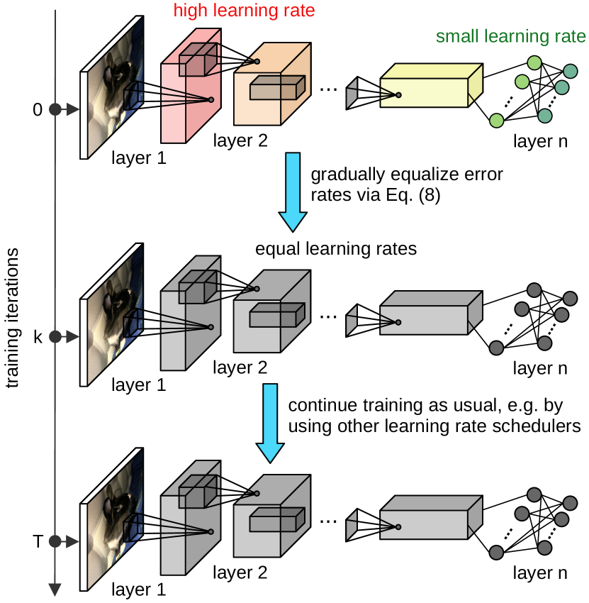
Figure 1: Training based on Learning Rate Curriculum.

Curriculum learning [1] refers to efficiently training effective neural networks by mimicking how humans learn, from easy to hard. As originally introduced by Bengio et al. [1], curriculum learning is a training procedure that first organizes the examples in their increasing order of difficulty, then starts the training of the neural network on the easiest examples, gradually adding increasingly more difficult examples along the way, until all training examples are fed to the network. The success of the approach relies in avoiding to force the learning of very difficult examples right from the beginning, instead guiding the model on the right path through the imposed curriculum. This type of curriculum is later referred to as data-level curriculum learning [2]. Indeed, Soviany et al. [2] identified several types of curriculum learning approaches in the literature, dividing them into four categories based on the components involved in the definition of machine learning given by Mitchell [3]. The four categories are: data-level curriculum (examples are presented from easy to hard), model-level curriculum (the modeling capacity of the network is gradually increased), task-level curriculum (the complexity of the learning task is increased during training), objective-level curriculum (the model optimizes towards an increasingly more complex objective). While data-level curriculum is the most natural and direct way to employ curriculum learning, its main disadvantage is that it requires a way to determine the difficulty of data samples. Despite having many successful applications [2, 4], there is no universal way to determine the difficulty of the data samples, making the data-level curriculum less applicable to scenarios where the difficulty is hard to estimate, e.g. classification of radar signals. The task-level and objective-level curriculum learning strategies suffer from similar issues, e.g. it is hard to create a curriculum when the model has to learn an easy task (binary classification) or the objective function is already convex.

Considering the above observations, we recognize the potential of model-level curriculum learning strategies of being applicable across a wider range of domains and tasks. To date, there are only a few works [5, 6, 7] in the category of pure model-level curriculum learning methods. However, these methods have some drawbacks caused by their domain-dependent or architecture-specific design. To benefit from the full potential of the model-level curriculum learning category, we propose LeRaC (Learning Rate Curriculum), a novel and simple curriculum learning approach which leverages the use of a different learning rate for each layer of a neural network to create a data-free curriculum during the initial training epochs. More specifically, LeRaC assigns higher learning rates to neural layers closer to the input, gradually decreasing the learning rates as the layers are placed farther away from the input. This prevents the propagation of noise caused by the random initialization of the network’s weights. The learning rates increase at various paces during the first training iterations, until they all reach the same value, as illustrated in Figure 1. From this point on, the neural model is trained as usual. This creates a model-level curriculum learning strategy that is applicable to any domain and compatible with any neural network, generating higher performance levels regardless of the architecture, without adding any extra training time. To the best of our knowledge, we are the first to employ a different learning rate per layer to achieve the same effect as conventional (data-level) curriculum learning.

We conduct comprehensive experiments on nine data sets from the computer vision (CIFAR-10 [8], CIFAR-100 [8], Tiny ImageNet [9], ImageNet-200 [9]), language (BoolQ [10], QNLI [11], RTE [11]) and audio (ESC-50 [12], CREMA-D [13]) domains, considering various convolutional (ResNet-18 [14], Wide-ResNet-50 [15], DenseNet-121 [16]), recurrent (LSTM [17]) and transformer (CvT [18], BERT [19], SepTr [20]) architectures, comparing our approach with the conventional training regime and Curriculum by Smoothing (CBS) [7], our closest competitor. Unlike CBS, our performance improvements over the standard training regime are consistent across all data sets and models. Furthermore, we significantly surpass CBS in terms of training time, since there is no additional cost over the conventional training regime for LeRaC, whereas CBS adds Gaussian kernel smoothing layers.

In summary, our contributions are twofold:

• We propose a novel and simple model-level curriculum learning strategy that creates a curriculum by updating the weights of each neural layer with a different learning rate, considering higher learning rates for the low-level feature layers and lower learning rates for the high-level feature layers.

• We empirically demonstrate the applicability to multiple domains (image, audio and text), the compatibility to several neural network architectures (convolutional neural networks, recurrent neural networks and transformers), and the time efficiency (no extra training time added) of LeRaC through a comprehensive set of experiments.

2 Related Work

Curriculum learning. Curriculum learning was initially introduced by Bengio et al. [1] as a training strategy that helps machine learning models to generalize better when the training examples are presented in the ascending order of their difficulty. Extensive surveys on curriculum learning methods, including the most recent advancements on the topic, were conducted by Soviany et al. [2] and Wang et al. [4]. In the former survey, Soviany et al. [2] emphasized that curriculum learning is not only applied at the data level, but also with respect to the other components involved in a machine learning approach, namely at the model level, the task level and the objective (loss) level. Regardless of the component on which curriculum learning is applied, the technique has demonstrated its effectiveness on a broad range of machine learning tasks, from computer vision [1, 21, 22, 23, 24, 25, 7] to natural language processing [26, 27, 28, 29, 1] and audio processing [30, 31].

The main challenge for the methods that build the curriculum at the data level is measuring the difficulty of the data samples, which is required to order the samples from easy to hard. Most studies have addressed the problem with human input [32, 33, 34] or metrics based on domain-specific heuristics. For instance, the text length [27, 35, 36, 37] and the word frequency [1, 29] have been employed in natural language processing. In computer vision, the samples containing fewer and larger objects have been considered to be easier in some works [24, 23]. Other solutions employed difficulty estimators [38] or even the confidence level of the predictions made by the neural network [39, 40] to approximate the complexity of the data samples.

The solutions listed above have shown their utility in specific application domains. Nonetheless, measuring the difficulty remains problematic when implementing standard (data-level) curriculum learning strategies, at least in some application domains. Therefore, several alternatives have emerged over time, handling the drawback and improving the conventional curriculum learning approach. In [41], the authors introduced self-paced learning to evaluate the learning progress when selecting the easy samples. The method was successfully employed in multiple settings [41, 42, 43, 44, 45, 46, 47]. Furthermore, some studies combined self-paced learning with the traditional pre-computed difficulty metrics [46, 48]. An additional advancement related to self-paced learning is the approach called self-paced learning with diversity [49]. The authors demonstrated that enforcing a certain level of variety among the selected examples can improve the final performance. Another set of methods that bypass the need for predefined difficulty metrics is known as teacher-student curriculum learning [50, 51]. In this setting, a teacher network learns a curriculum to supervise a student neural network.

Closer to our work, a few methods [6, 7, 5] proposed to apply curriculum learning at the model level, by gradually increasing the learning capacity (complexity) of the neural architecture. Such curriculum learning strategies do not need to know the difficulty of the data samples, thus having a great potential to be useful in a broad range of tasks. For example, Karras et al. [6] proposed to gradually add layers to generative adversarial networks during training, while increasing the resolution of the input images at the same time. They are thus able to generate realistic high-resolution images. However, their approach is not applicable to every domain, since there is no notion of resolution for some input data types, e.g. text. Sinha et al. [7] presented a strategy that blurs the activation maps of the convolutional layers using Gaussian kernel layers, reducing the noisy information caused by the network initialization. The blur level is progressively reduced to zero by decreasing the standard deviation of the Gaussian kernels. With this mechanism, they obtain a training procedure that allows the neural network to see simple information at the start of the process and more intricate details towards the end. Curriculum by Smoothing (CBS) [7] was only shown to be useful for convolutional architectures applied in the image domain. Although we found that CBS is applicable to transformers by blurring the tokens, it is not necessarily applicable to any neural architecture, e.g. standard feed-forward neural networks. As an alternative to CBS, Burduja et al. [5] proposed to apply the same smoothing process on the input image instead of the activation maps. The method was applied with success in medical image alignment. However, this approach is not applicable to natural language input, as it it not clear how to apply the blurring operation on the input text.

Different from Burduja et al. [5] and Karras et al. [6], our approach is applicable to various domains, including but not limited to natural language processing, as demonstrated throughout our experiments. To the best of our knowledge, the only competing model-level curriculum method which is applicable to various domains is CBS [7]. Unlike CBS, LeRaC does not introduce new operations, such as smoothing with Gaussian kernels, during training. As such, our approach does not increase the training time with respect to the conventional training regime, as later shown in the experiments. In summary, we consider that the simplicity of our approach comes with many important advantages: applicability to any domain and task, compatibility with any neural network architecture, time efficiency (adds no extra training time). We support all these claims through the comprehensive experiments presented in Section 4.

Relation to learning rate schedulers. The are other contributions [52, 53] showing that using adaptive learning rates can lead to improved results. We explain how our method is different below. In [52], the main goal is increasing the learning rate of certain layers as necessary, to escape saddle points. Different from [52], our strategy reduces the learning rates of deeper layers, introducing soft optimization restrictions in the initial training epochs. You et al. [53] proposed to train models with very large batches using a learning rate for each layer, by scaling the learning rate with respect to the norms of the gradients. The goal of You et al. [53] is to specifically learn models with large batch sizes, e.g. formed of 8K samples. Unlike [53], we propose a more generic approach that can be applied to multiple architectures (convolutional, recurrent, transformer) under unrestricted training settings.

Gotmare et al. [54] point out that learning rate with warmup restarts is an effective strategy to improve stability of training neural models using large batches. Different from LeRaC, this approach does not employ a different learning rate for each layer. Moreover, the strategy restarts the learning rate at different moments during the entire training process, while LeRaC is applied only during the first few training epochs. Aside from these technical differences, our experiments already include a direct comparison of the two strategies for the CvT architecture. The results show that introducing LeRaC brings consistent improvements. We thus conclude that our strategy is a viable and distinct alternative to learning rate warmup with restarts.

Relation to optimizers. We consider Adam [55] and related optimizers as orthogonal approaches that perform the optimization rather than setting the learning rate. Our approach, LeRaC, only aims to guide the optimization during the initial training iterations by reducing the relevance of deeper network layers. Most of the baseline architectures used in our experiments are already based on Adam or some of its variations, e.g. AdaMax, AdamW [56]. LeRaC is applied in conjunction with these optimizers, showing improved performance over various architectures and application domains. This supports our claim that LeRaC is an orthogonal contribution to the family of Adam optimizers.

3 Method

Deep neural networks are commonly trained on a set of labeled data samples denoted as:

$$S=\{(x_{i},y_{i})|x_{i}\in X,y_{i}\in Y,\forall i\in\{1,2,...,m\}\},$$ (1)

where $m$ is the number of examples, $x_{i}$ is a data sample and $y_{i}$ is the associated label. The training process of a neural network $f$ with parameters $\theta$ consists of minimizing some objective (loss) function $\mathcal{L}$ that quantifies the differences between the ground-truth labels and the predictions of the model $f$:

$$\min_{\theta}\frac{1}{m}\sum_{i=1}^{m}\mathcal{L}\left(y_{i},f(x_{i},\theta)\right).$$ (2)

The optimization is generally performed by some variant of Stochastic Gradient Descent (SGD), where the gradients are back-propagated from the neural layers closer to the output towards the neural layers closer to input through the chain rule. Let $f_{1}$, $f_{2}$, …., $f_{n}$ and $\theta_{1}$, $\theta_{2}$, …, $\theta_{n}$ denote the neural layers and the corresponding weights of the model $f$, such that the weights $\theta_{j}$ belong to the layer $f_{j}$, $\forall j\in\{1,2,...,n\}$. The output of the neural network for some training data sample $x_{i}\in X$ is formally computed as follows:

$$\hat{y}_{i}=f(x_{i},\theta)=f_{n}\left(...f_{2}\left(f_{1}\left(x_{i},\theta_{1}\right),\theta_{2}\right)....,\theta_{n}\right).$$ (3)

To optimize the model via SGD, the weights are updated as follows:

$$\theta_{j}^{(t+1)}=\theta_{j}^{(t)}-\eta^{(t)}\cdot\frac{\partial\mathcal{L}}{\partial\theta_{j}^{(t)}},\forall j\in\{1,2,...,n\},$$ (4)

where $t$ is the index of the current training iteration, $\eta^{(t)}>0$ is the learning rate at iteration $t$, and the gradient of $\mathcal{L}$ with respect to $\theta_{j}^{(t)}$ is computed via the chain rule. Before starting the training process, the weights $\theta_{j}^{(0)}$ are commonly initialized with random values.

Due to the random initialization of the weights, the information propagated through the neural model during the early training iterations can contain a large amount of noise, which can negatively impact the learning process, as discussed by Sinha et al. [7]. Due to the feed-forward processing, we conjecture that the noise level tends to grow with each neural layer, from $f_{j}$ to $f_{j+1}$ (the empirical proof is provided in the supplementary). The same issue can occur if the weights are pre-trained on a distinct task, where the misalignment of the weights with a new task is likely higher for the high-level (specialized) feature layers. To alleviate this problem, we propose to introduce a curriculum learning strategy that assigns a different learning rate $\eta_{j}$ to each layer $f_{j}$, as follows:

$$\theta_{j}^{(t+1)}=\theta_{j}^{(t)}-\eta_{j}^{(t)}\cdot\frac{\partial\mathcal{L}}{\partial\theta_{j}^{(t)}},\forall j\in\{1,2,...,n\},$$ (5)

such that:

$$\eta^{(0)}\geq\eta_{1}^{(0)}\geq\eta_{2}^{(0)}\geq...\geq\eta_{n}^{(0)},$$ (6)

$$\eta^{(k)}=\eta_{1}^{(k)}=\eta_{2}^{(k)}=...=\eta_{n}^{(k)},$$ (7)

where $\eta_{j}^{(0)}$ are the initial learning rates and $\eta_{j}^{(k)}$ are the updated learning rates at iteration $k$. The condition formulated in Eq. (6) indicates that the initial learning rate $\eta_{j}^{(0)}$ of a neural layer $f_{j}$ gets lower as the level of the respective neural layer becomes higher (farther away from the input). With each training iteration $t\leq k$, the learning rates are gradually increased, until they become equal, according to Eq. (7). Thus, our curriculum learning strategy is only applied during the early training iterations, where the noise caused by the random weight initialization is most prevalent. Hence, $k$ is a hyperparameter of LeRaC that is usually adjusted such that $k\ll T$, where $T$ is the total number of training iterations. In practice, we obtain optimal results by running LeRaC up to any epoch between $2$ and $7$.

We increase each learning rate $\eta_{j}$ from iteration $0$ to iteration $k$ using an exponential scheduler that is based on the following rule:

$$\eta_{j}^{(l)}=\eta_{j}^{(0)}\cdot c^{\frac{l}{k}\cdot\left(\log_{c}\eta_{j}^{(k)}-\log_{c}\eta_{j}^{(0)}\right)},\forall l\in\{0,1,...,k\}.$$ (8)

We set $c=10$ in Eq. (8) across all our experiments. In practice, we obtain optimal results by initializing the lowest learning rate $\eta_{n}^{(0)}$ with a value that is around five or six orders of magnitude lower than $\eta^{(0)}$, while the highest learning rate $\eta_{1}^{(0)}$ is usually equal to $\eta^{(0)}$. Apart from these general practical notes, the exact LeRaC configuration for each neural architecture is established by tuning the hyperparameters on the available validation sets.

We underline that the output feature maps of a layer $j$ are affected $(i)$ by the initial random weights (noise) $\theta_{j}^{(0)}$ of the respective layer, and $(ii)$ by the input feature maps, which are in turn affected by the random weights of the previous layers $\theta_{1}^{(0)},...,\theta_{j-1}^{(0)}$. Hence, the noise affecting the feature maps increases with each layer processing the feature maps, being multiplied with the weights from each layer along the way. Our curriculum learning strategy imposes the training of the earlier layers at a faster pace, transforming the noisy weights into discriminative patterns. As noise from the earlier layer weights is eliminated, we train the later layers at faster and faster paces, until all learning rates become equal at epoch $k$.

From a technical point of view, we note that our approach can also be regarded as a way to guide the optimization, which we see as an alternative to loss function smoothing. The link between curriculum learning and loss smoothing is mentioned in [2], where the authors suggest that curriculum learning strategies induce a smoothing of the loss function, where the smoothing is higher during the early training iterations (simplifying the optimization) and lower to non-existent during the late training iterations (restoring the complexity of the loss function). LeRaC is aimed at producing a similar effect, but in a softer manner by dampening the importance of optimizing the weights of high-level layers in the early training iterations. Additionally, we empirically observe (see results in the supplementary) that LeRaC tends to balance the training pace of low-level and high-level features, while the conventional regime seems to update the high-level layers at a faster pace. This could provide an additional intuitive explanation of why our method works.

4 Experiments

4.1 Data Sets

In general, we adopt the official data splits for the nine benchmarks considered in our experiments. When a validation set is not available, we keep $10\%$ of the training data for validation.

CIFAR-10. CIFAR-10 [8] is a popular data set for object recognition in images. It consists of 60,000 color images with a resolution of $32\times 32$ pixels. An images depicts one of 10 object classes, each class having 6,000 examples. We use the official data split with a training set of 50,000 images and a test set of 10,000 images.

CIFAR-100. The CIFAR-100 [8] data set is similar to CIFAR-10, except that it has 100 classes with 600 images per class. There are 50,000 training images and 10,000 test images.

Tiny ImageNet. Tiny ImageNet is a subset of ImageNet-1K [9] which provides 100,000 training images, 25,000 validation images and 25,000 test images representing objects from 200 different classes. The size of each image is $64\times 64$ pixels.

ImageNet-200. ImageNet-200 is a part of ImageNet-1K [9] with images from a subset of 200 classes, where the original resolution of the images is preserved.

BoolQ. BoolQ [10] is a question answering data set for yes/no questions containing 15,942 examples. The questions are naturally occurring, being generated in unprompted and unconstrained settings. Each example is a triplet of the form: {question, passage, answer}. We use the data split provided in the SuperGLUE benchmark [57], containing 9,427 examples for training, 3,270 for validation and 3,245 for testing.

QNLI. The QNLI (Question-answering NLI) data set [11] is a natural language inference benchmark automatically derived from SQuAD [58]. The data set contains {question, sentence} pairs and the task is to determine whether the context sentence contains the answer to the question. The data set is constructed on top of Wikipedia documents, each document being accompanied, on average, by 4 questions. We consider the data split provided in the GLUE benchmark [11], which comprises 104,743 examples for training, 5,463 for validation and 5,463 for testing.

RTE. Recognizing Textual Entailment (RTE) [11] is a natural language inference data set containing pairs of sentences with the target label indicating if the meaning of one sentence can be inferred from the other. The training subset includes 2,490 samples, the validation set 277, and the test set 3,000 examples.

CREMA-D. The CREMA-D multi-modal database [13] is formed of 7,442 videos of 91 actors (48 male and 43 female) of different ethnic groups. The actors perform various emotions while uttering 12 particular sentences that evoke one of the 6 emotion categories: anger, disgust, fear, happy, neutral, and sad. Following [47], we conduct experiments only on the audio modality, dividing the set of audio samples into $70\%$ for training, $15\%$ for validation and $15\%$ for testing.

ESC-50. The ESC-50 [12] data set is a collection of 2,000 samples of 5 seconds each, comprising 50 classes of various common sound events. Samples are recorded at a 44.1 kHz sampling frequency, with a single channel. In our evaluation, we employ the 5-fold cross-validation procedure, as described in related works [12, 20].

4.2 Experimental Setup

Architectures. To demonstrate the compatibility of LeRaC with multiple neural architectures, we select several convolutional, recurrent and transformer models. As representative convolutional neural networks (CNNs), we opt for ResNet-18 [14], Wide-ResNet-50 [15] and DenseNet-121 [16]. As representative transformers, we consider CvT-13 [18], BERT${}_{\mbox{\scriptsize{uncased-large}}}$ [19] and SepTr [20]. For CvT, we consider both pre-trained and randomly initialized versions. We use an uncased large pre-trained version of BERT. As Ristea et al. [20], we train SepTr from scratch. In addition, we employ a long short-term memory (LSTM) network [17] to represent recurrent neural networks (RNNs). The recurrent neural network contains two LSTM layers, each having a hidden dimension of 256 components. These layers are preceded by one embedding layer with the embedding size set to 128 elements. The output of the last recurrent layer is passed to a classifier comprised of two fully connected layers. The LSTM is activated by rectified linear units (ReLU). We apply the aforementioned models on distinct input data types, considering the intended application domain of each model. Hence, ResNet-18, Wide-ResNet-50 and CvT are applied on images, BERT and LSTM are applied on text, and SepTr and DenseNet-121 are applied on audio.

Baselines. We compare LeRaC with two baselines: the conventional training regime (which uses early stopping and reduces the learning rate on plateau) and the state-of-the-art Curriculum by Smoothing [7]. For CBS, we use the official code released by Sinha et al. [7] at https://github.com/pairlab/CBS, to ensure the replicability of their method in our experimental settings, which include a more diverse selection of input data types and neural architectures.

Architecture	Optimizer	Mini-batch	#Epochs	$\eta^{(0)}$	CBS				LeRaC
					$\sigma$	$d$	$u$		$k$	$\eta_{1}^{(0)}$ - $\eta_{n}^{(0)}$
ResNet-18	SGD	64	100-200	$10^{-1}$	1	0.9	2-5		5-7	$10^{-1}$ - $10^{-8}$
Wide-ResNet-50	SGD	64	100-200	$10^{-1}$	1	0.9	2-5		5-7	$10^{-1}$ - $10^{-8}$
CvT-13	AdaMax	64-128	150-200	$2\!\cdot\!10^{-3}$	1	0.9	2-5		2-5	$2\!\cdot\!10^{-3}$ - $2\!\cdot\!10^{-8}$
CvT-13${}_{\mbox{\scriptsize{pre-trained}}}$	AdaMax	64-128	25	$5\!\cdot\!10^{-4}$	1	0.9	2-5		3-6	$5\!\cdot\!10^{-4}$ - $5\!\cdot\!10^{-10}$
BERT${}_{\mbox{\scriptsize{large-uncased}}}$	AdaMax	10	7-25	$5\!\cdot\!10^{-5}$	1	0.9	1		3	$5\!\cdot\!10^{-5}$ - $5\!\cdot\!10^{-8}$
LSTM	AdamW	256-512	25-70	$10^{-3}$	1	0.9	2		3-4	$10^{-3}$ - $10^{-7}$
SepTR	Adam	2	50	$10^{-4}$	0.8	0.9	1-3		2-5	$10^{-4}$ - $10^{-8}$
DenseNet-121	Adam	64	50	$10^{-4}$	0.8	0.9	1-3		2-5	$10^{-4}$ - $5\!\cdot\!10^{-8}$

Table 1: Optimal hyperparameter settings for the various neural architectures used in our experiments.

Hyperparameter tuning. We tune all hyperparameters on the validation set of each benchmark. In Table 1, we present the optimal hyperparameters chosen for each architecture. In addition to the standard parameters of the training process, we report the parameters that are specific for the CBS and LeRaC strategies. In the case of CBS, $\sigma$ denotes the standard deviation of the Gaussian kernel, $d$ is the decay rate for $\sigma$, and $u$ is the decay step. Regarding the parameters of LeRaC, $k$ represents the number of iterations used in Eq. (8), and $\eta_{1}^{(0)}$ and $\eta_{n}^{(0)}$ are the initial learning rates for the first and last layers of the architecture, respectively. We underline that $\eta_{1}^{(0)}=\eta^{(0)}$ and $c=10$, in all experiments. Moreover, $\eta_{j}^{(k)}=\eta^{(0)}$, i.e. the initial learning rates of LeRaC converge to the original learning rate set for the conventional training regime. All models are trained with early stopping and the learning rate is reduced by a factor of $10$ when the loss reaches a plateau.

Evaluation. We evaluate all models in terms of the classification accuracy. We repeat the training process of each model for 5 times and report the average accuracy and the standard deviation.

Image preprocessing. For the image classification experiments, we apply the same data preprocessing approach as Sinha et al. [7]. Hence, we normalize the images and maintain their original resolution, $32\times 32$ pixels for CIFAR-10 and CIFAR-100, and $64\times 64$ pixels for Tiny ImageNet. Similar to Sinha et al. [7], we do not employ data augmentation.

Text preprocessing. For the text classification experiments with BERT, we lowercase all words and add the classification token ([CLS]) at the start of the input sequence. We add the separator token ([SEP]) to delimit sentences. For the LSTM network, we lowercase all words and replace them with indexes from vocabularies constructed from the training set. The input sequence length is limited to $512$ tokens for BERT and $200$ tokens for LSTM.

Speech preprocessing. We transform each audio sample into a time-frequency matrix by computing the discrete Short Time Fourier Transform (STFT) with $N_{x}$ FFT points, using a Hamming window of length $L$ and a hop size $R$. For CREMA-D, we first standardize all audio clips to a fixed dimension of $4$ seconds by padding or clipping the samples. Then, we apply the STFT with $N_{x}=1024$, $R=64$ and a window size of $L=512$. For ESC-50, we keep the same values for $N_{x}$ and $L$, but we increase the hop size to $R=128$. Next, for each STFT, we compute the square root of the magnitude and map the values to $128$ Mel bins. The result is converted to a logarithmic scale and normalized to the interval $[0,1]$. Furthermore, in all our speech classification experiments, we use the following data augmentation methods: noise perturbation, time shifting, speed perturbation, mix-up and SpecAugment [59]. The speech preprocessing steps are carried out following Ristea et al. [20].

Architecture	Training Regime	CIFAR-10	CIFAR-100	Tiny ImageNet	ImageNet-200
	conventional	$89.20\pm 0.43$	$65.28\pm 0.16$	$57.41\pm 0.05$	$71.66\pm 0.10$
ResNet-18	CBS [7]	$89.53\pm 0.22$	$\mathbf{66.41}\pm 0.21$	$55.49\pm 0.20$	$72.51\pm 0.15$
	LeRaC (ours)	$\mathbf{89.56}\pm 0.16$	$66.02\pm 0.17$	$\mathbf{57.86}\pm 0.20$	$\mathbf{72.93}\pm 0.17$
	conventional	$91.22\pm 0.24$	$68.14\pm 0.16$	$55.97\pm 0.30$	$72.83\pm 0.13$
Wide-ResNet-50	CBS [7]	$89.05\pm 1.00$	$65.73\pm 0.36$	$48.30\pm 1.53$	$\mathbf{74.75}\pm 0.08$
	LeRaC (ours)	$\mathbf{91.58}\pm 0.16$	$\mathbf{69.38}\pm 0.26$	$\mathbf{56.48}\pm 0.60$	$74.38\pm 0.14$
	conventional	$71.84\pm 0.37$	$41.87\pm 0.16$	$33.38\pm 0.27$	$70.68\pm 0.17$
CvT-13	CBS [7]	$72.64\pm 0.29$	$\mathbf{44.48}\pm 0.40$	$33.56\pm 0.36$	$69.91\pm 0.10$
	LeRaC (ours)	$\mathbf{72.90}\pm 0.28$	$43.46\pm 0.18$	$\mathbf{33.95}\pm 0.28$	$\mathbf{70.87}\pm 0.13$
	conventional	$93.56\pm 0.05$	$77.80\pm 0.16$	$70.71\pm 0.35$	-
CvT-13${}_{\mbox{\scriptsize{pre-trained}}}$	CBS [7]	$85.85\pm 0.15$	$62.35\pm 0.48$	$68.41\pm 0.13$	-
	LeRaC (ours)	$\mathbf{94.15}\pm 0.03$	$\mathbf{78.93}\pm 0.05$	$\mathbf{71.34}\pm 0.08$	-

Table 2: Average accuracy rates (in %) over 5 runs on CIFAR-10, CIFAR-100, Tiny ImageNet and ImageNet-200 for various neural models based on different training regimes: conventional, CBS [7] and LeRaC. The accuracy of the best training regime in each experiment is highlighted in bold.

Architecture	Training Regime	BoolQ	RTE	QNLI
	conventional	$74.12\pm 0.32$	$74.48\pm 1.36$	$92.13\pm 0.08$
BERT${}_{\mbox{\scriptsize{large-uncased}}}$	CBS [7]	$74.37\pm 1.11$	$74.97\pm 1.96$	$91.47\pm 0.22$
	LeRaC (ours)	$\mathbf{75.55}\pm 0.66$	$\mathbf{75.81}\pm 0.29$	$\mathbf{92.45}\pm 0.13$
	conventional	$64.40\pm 1.37$	$54.12\pm 1.60$	$59.42\pm 0.36$
LSTM	CBS [7]	$64.75\pm 1.54$	$54.03\pm 0.45$	$59.89\pm 0.38$
	LeRaC (ours)	$\mathbf{65.80}\pm 0.33$	$\mathbf{55.71}\pm 1.04$	$\mathbf{59.98}\pm 0.34$

Table 3: Average accuracy rates (in %) over 5 runs on BoolQ, RTE and QNLI for BERT and LSTM based on different training regimes: conventional, CBS [7] and LeRaC. The accuracy of the best training regime in each experiment is highlighted in bold.

4.3 Results

Image classification. In Table 2, we present the image classification results on CIFAR-10, CIFAR-100, Tiny ImageNet and ImageNet-200. Since CvT-13 is pre-trained on ImageNet, it does not make sense to fine-tune it on ImageNet-200. Thus, the respective results are not reported. On the one hand, there are three scenarios (ResNet-18 on CIFAR-100, Wide-ResNet-50 on ImageNet-200, and CvT-13 on CIFAR-100) in which CBS provides the largest improvements over the conventional regime, surpassing LeRaC in the respective cases. On the other hand, there are eight scenarios where CBS degrades the accuracy with respect to the standard training regime. This shows that the improvements attained by CBS are inconsistent across models and data sets. Unlike CBS, our strategy surpasses the baseline regime in all fifteen cases, thus being more consistent. In six of these cases, the accuracy gains of LeRaC are higher than $1\%$. Moreover, LeRaC outperforms CBS in twelve out of fifteen cases. We thus consider that LeRaC can be regarded as a better choice than CBS, bringing consistent performance gains.

Text classification. In Table 3, we report the text classification results on BoolQ, RTE and QNLI. Here, there are only two cases (BERT on QNLI and LSTM on RTE) where CBS leads to performance drops compared to the conventional training regime. In all other cases, the improvements of CBS are below $0.6\%$. Just as in the image classification experiments, LeRaC brings accuracy gains for each and every model and data set. In four out of six scenarios, the accuracy gains yielded by LeRaC are higher than $1.3\%$. Once again, LeRaC proves to be the best and most consistent regime, generally outperforming CBS by significant margins.

Architecture	Training Regime	CREMA-D	ESC-50
	conventional	$70.47\!\pm\!0.67$	$91.13\!\pm\!0.33$
SepTr	CBS [7]	$69.98\!\pm\!0.71$	$91.15\!\pm\!0.41$
	LeRaC (ours)	$\mathbf{70.95}\!\pm\!0.56$	$\mathbf{91.58}\!\pm\!0.28$
	conventional	$67.21\!\pm\!0.12$	$88.91\!\pm\!0.11$
DenseNet-121	CBS [7]	$68.16\!\pm\!0.19$	$88.76\!\pm\!0.17$
	LeRaC (ours)	$\mathbf{68.99}\!\pm\!0.08$	$\mathbf{90.02}\!\pm\!0.10$

Table 4: Average accuracy rates (in %) over 5 runs on CREMA-D and ESC-50 for SepTr and DenseNet-121 based on different training regimes: conventional, CBS [7] and LeRaC. The accuracy of the best training regime in each experiment is highlighted in bold.

Architecture	Training Regime	CIFAR-10	CIFAR-100	Tiny ImageNet
	conventional	$71.84\pm 0.37$	$41.87\pm 0.16$	$33.38\pm 0.27$
	CBS [7]	$72.64\pm 0.29$	$44.48\pm 0.40$	$33.56\pm 0.36$
CvT-13	LeRac (linear update)	$72.49\pm 0.27$	$43.39\pm 0.14$	$33.86\pm 0.07$
	LeRaC (exponential update)	$72.90\pm 0.28$	$43.46\pm 0.18$	$33.95\pm 0.28$
	CBS [7] + LeRaC	$73.25\pm 0.19$	$44.90\pm 0.41$	$34.20\pm 0.61$

Table 5: Average accuracy rates (in %) over 5 runs on CIFAR-10, CIFAR-100 and Tiny ImageNet for CvT-13 based on different training regimes: conventional, CBS [7], LeRaC with linear update, LeRaC with exponential update (proposed), and a combination of CBS and LeRaC.

Speech classification. In Table 4, we present the results obtained on the audio data sets, namely CREMA-D and ESC-50. We observe that the CBS strategy obtains lower results compared with the baseline in two cases (SepTr on CREMA-D and DenseNet-121 on ESC-50), while our method provides superior results for each and every case. By applying LeRaC on SepTr, we set a new state-of-the-art accuracy level ($70.95\%$) on the CREMA-D audio modality, surpassing the previous state-of-the-art value attained by Ristea et al. [20] with SepTr alone. When applied on DenseNet-121, LeRaC brings performance improvements higher than $1\%$, the highest improvement ($1.78\%$) over the baseline being attained on CREMA-D.

Additional results. An interesting aspect worth studying is to determine if putting the CBS and LeRaC regimes together could bring further performance gains. We study the effect of combining CBS and LeRaC for CvT-13, since there are three data sets for which both CBS and LeRaC improve CvT-13 (see Table 2). The corresponding results are shown in Table 5. The reported results show that the combination brings accuracy gains across all three data sets (CIFAR-10, CIFAR-100, Tiny ImageNet). We thus conclude that the combination of curriculum learning regimes is worth a try, whenever the two independent regimes boost performance.

Another important aspect is to establish if the exponential learning rate update proposed in Eq. (8) is a good choice. To test this out, we keep the CvT-13 model and change the LeRaC regime to use a linear update of the learning rate. We observe performance gains with both types of update rules, but our exponential learning rate update seems to bring higher gains on all three data sets. We thus conclude that the update rule defined in Eq. (8) is a sound option.

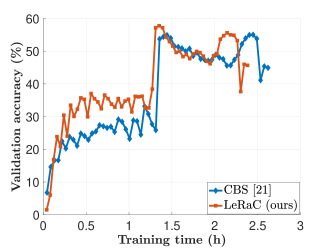
(a) ResNet-18 on Tiny ImageNet.

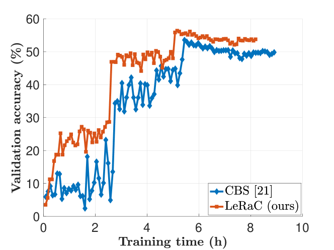
(b) Wide-ResNet-50 on Tiny ImageNet.

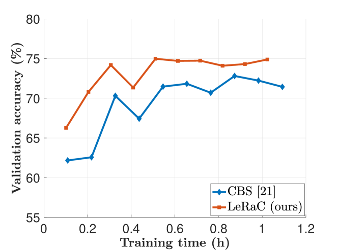
(c) BERT on BoolQ.

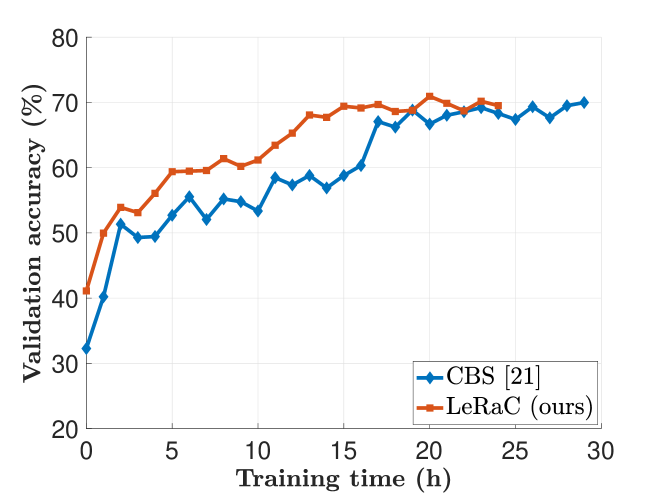
(d) SepTr on CREMA-D.

Figure 2: Validation accuracy (on the y-axis) versus training time (on the x-axis) for four distinct architectures. The number of training epochs is the same for both LeRaC and CBS, the observable time difference being caused by the overhead of CBS due to the Gaussian kernel layers.

Training time comparison. For a particular model and data set, all training regimes are executed for the same number of epochs, for a fair comparison. However, the CBS strategy adds the smoothing operation at multiple levels inside the architecture, which increases the training time. To this end, we compare the training time (in hours) versus the validation error of CBS and LeRaC. For this experiment, we selected four neural models and illustrate the evolution of the validation accuracy over time in Figure 2. We underline that LeRaC introduces faster convergence times, being around 7-12% faster than CBS. It is trivial to note that LeRaC requires the same time as the conventional regime.

Ablation results. We present several ablation results in the supplementary.

5 Conclusion

In this paper, we introduced a novel model-level curriculum learning approach that is based on starting the training process with increasingly lower learning rates per layer, as the layers get closer to the output. We conducted comprehensive experiments on nine data sets from three domains (image, text and audio), considering multiple neural architectures (CNNs, RNNs and transformers), to compare our novel training regime (LeRaC) with a state-of-the-art regime (CBS [7]) as well as the conventional training regime (based on early stopping and reduce on plateau). The empirical results demonstrate that LeRaC is significantly more consistent than CBS, perhaps being the most versatile curriculum learning strategy to date, due to its compatibility with multiple neural models and its usefulness across different domains. Remarkably, all these benefits come for free, i.e. LeRaC does not add any extra time over the conventional approach.

Acknowledgements. Work funded by UEFISCDI through project number PN-III-P1-1.1-TE-2019-0235.

6 Supplementary

In the supplementary, we present a series of ablation and extra experiments to validate several choices and statements in our paper. Additionally, we clarify some important aspects and discuss the limitations of our work.

6.1 Additional and Ablation Results

Significance testing. To determine if the reported accuracy gains observed for LeRaC with respect to the baseline are significant, we apply McNemar significance testing [60] to the results reported in the main article on all nine data sets. In 19 of 25 cases, we found that our results are significantly better than the corresponding baseline, at a confidence threshold of $0.001$. This confirms that our gains are statistically significant in the majority of cases.

Noise quantification of early and later layers. The application of LeRaC is justified by the fact that the level of noise gradually grows with each layer during a forward pass through a neural network with randomly initialized weights. To empirically confirm this conjecture, we have computed the distances for the low-level (first conv) and high-level (last conv) layers between the activation maps at iteration $0$ (based on random weights) and the last iteration (based on weights optimized until convergence) for ResNet-18 on CIFAR-10, while using the conventional training regime. The computed distances shown in Table 6 confirm our conjecture, namely that shallow layers contain less noise than deep layer when applying the conventional training regime.

Entropy of low-level versus high-level features. We showed a few examples of training dynamics in Fig. 2 from the main article. All four graphs exhibit a higher gap between standard training and LeRaC in the first half of the training process, suggesting that LeRaC has an important role towards faster convergence. To assess the comparative quality of low-level versus high-level feature maps obtained either with conventional or LeRaC training, we compute the entropy of the first and last conv layers of ResNet-18 on CIFAR-10, after $k=6$ iterations. We report the computed entropy levels in Table 7. Conventional training seems to update deeper layers faster, observing a higher difference between the entropy levels of low-level and high-level features obtained with conventional training than with LeRac. This shows that LeRaC balances the training pace of low-level and high-level features. We conjecture that updating the deeper layers too soon could lead to overfitting to the noise still present in the early layers. This statement is supported by our empirical results on nine data sets, showing that giving a chance to the early layers to converge before introducing large updates to the later layers leads to superior performance.

Training Regime	Distance
	First Conv Layer	Last Conv Layer
conventional	$38.36$	$709.93$

Table 6: Distances between feature maps at epoch $k=0$ and feature maps after the final epoch for ResNet-18 on CIFAR-10, while using the conventional training regime. Distances are independently computed for the first and last convolutional layers.

Training Regime	Entropy
	First Conv Layer	Last Conv Layer
conventional	$0.9965$	$0.9905$
LeRaC (ours)	$0.9970$	$0.9968$

Table 7: Entropy after $k=6$ epochs for ResNet-18 on CIFAR-10, while alternating between the conventional and LeRaC training regimes.

Training Regime	Distance
	First Conv Layer	Last Conv Layer
conventional	$0.60$	$0.37$
LeRaC (ours)	$0.61$	$0.66$

Table 8: Distances between feature maps at epoch $k=6$ and feature maps after the final epoch for ResNet-18 on CIFAR-10, while alternating between the conventional and LeRaC training regimes. Distances are independently computed for the first and last convolutional layers.

Data Set	Architecture	Training Regime	$\eta_{1}^{(0)}$-$\eta_{n}^{(0)}$	Accuracy
CIFAR-100	ResNet-18	conventional	$10^{-1}$-$10^{-1}$	$65.28\!\pm\!0.16$
		LeRaC (ours)	$10^{-1}$-$10^{-6}$	$\mathbf{65.82}\!\pm\!0.08$
			$10^{-1}$-$10^{-7}$	$\mathbf{65.80}\!\pm\!0.16$
			$10^{-1}$-$10^{-8}$	$\mathbf{66.02}\!\pm\!0.17$
			$10^{-1}$-$10^{-9}$	$\mathbf{65.59}\!\pm\!0.49$
			$10^{-1}$-$10^{-10}$	$\mathbf{65.76}\!\pm\!0.22$
			$10^{-2}$-$10^{-8}$	$\mathbf{65.71}\!\pm\!0.08$
			$10^{-3}$-$10^{-8}$	$65.25\!\pm\!0.12$
	Wide-ResNet-50	conventional	$10^{-1}$-$10^{-1}$	$68.14\!\pm\!0.16$
		LeRaC (ours)	$10^{-1}$-$10^{-6}$	$\mathbf{68.64}\!\pm\!0.52$
			$10^{-1}$-$10^{-7}$	$\mathbf{69.25}\!\pm\!0.37$
			$10^{-1}$-$10^{-8}$	$\mathbf{69.38}\!\pm\!0.26$
			$10^{-1}$-$10^{-9}$	$\mathbf{69.26}\!\pm\!0.27$
			$10^{-1}$-$10^{-10}$	$\mathbf{69.66}\!\pm\!0.34$
			$10^{-2}$-$10^{-8}$	$\mathbf{68.51}\!\pm\!0.52$
			$10^{-3}$-$10^{-8}$	$\mathbf{68.71}\!\pm\!0.47$
CREMA-D	SepTr	conventional	$10^{-4}$-$10^{-4}$	$70.47\!\pm\!0.67$
		LeRaC (ours)	$10^{-2}$-$10^{-8}$	$\mathbf{70.74}\!\pm\!0.55$
			$10^{-3}$-$10^{-8}$	$\mathbf{70.91}\!\pm\!0.49$
			$10^{-4}$-$10^{-8}$	$\mathbf{70.95}\!\pm\!0.56$
			$10^{-5}$-$10^{-8}$	$70.32\!\pm\!0.57$
			$10^{-4}$-$10^{-7}$	$\mathbf{70.49}\!\pm\!0.44$
			$10^{-4}$-$10^{-9}$	$\mathbf{70.58}\!\pm\!0.48$

Table 9: Average accuracy rates (in %) over 5 runs for ResNet-18 and Wide-ResNet-50 on CIFAR-100, as well as SepTr on CREMA-D, based on different ranges for the initial learning rates. The accuracy rates surpassing the baseline training regime are highlighted in bold.

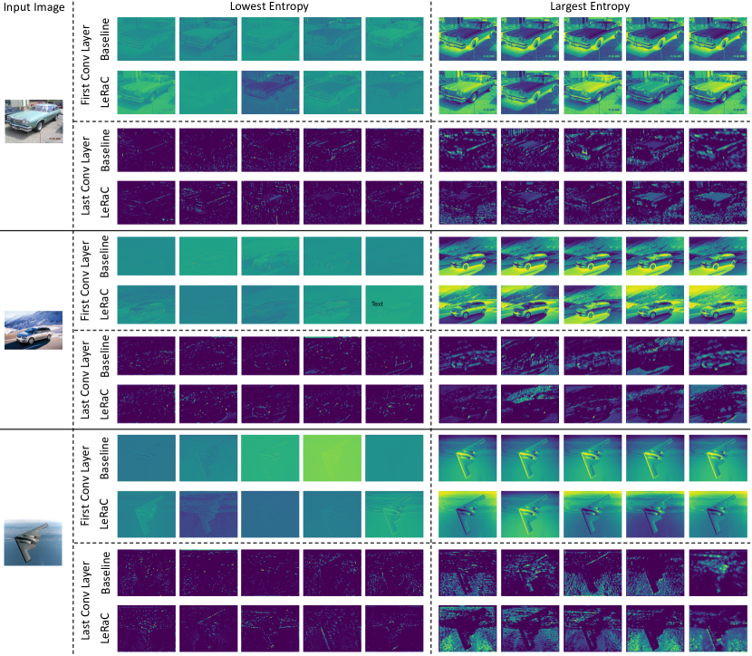
Figure 3: Activation maps with low and high entropy from the first and last conv layers of ResNet-18 trained on CIFAR-10 for $k=6$ epochs with the conventional (baseline) and LeRaC (ours) regimes. The input images are taken from ImageNet. Best viewed in color.

Aside from computing the global entropy over all training samples, in Figure 3, we illustrate some activation maps with the highest and lowest entropy from the first and last conv layers for three randomly chosen examples from ImageNet. The activation maps are extracted at epoch $k=6$ from the ResNet-18 model trained on CIFAR-10 either with the conventional regime or the LeRaC regime. In general, we observe that the low-level activation maps corresponding to LeRaC exhibit a higher degree of variability (being more distinct from each other), regardless of the entropy level (low or high). We believe the higher degree of variability comes from the fact that, having lower learning rates for the deeper layers, the model based on LeRaC is likely focused on finding a higher variety of patterns within the first layers to minimize the loss. For the third example (the image of an airplane), we observe that the activation maps with the highest entropy from the last conv layer produced by LeRaC have a higher entropy than the activation maps with the highest entropy produced by the conventional regime. This observation is in line with the results reported in Table 7, confirming that LeRaC is able to better balance the entropy of low-level and high-level features by preventing the faster convergence of the deeper layers.

Distances at epoch $\mathbf{k}$ versus final epoch. In Table 7, we report the entropy of the low-level and high-level layers after $k=6$ epochs, before and after using LeRaC to train ResNet-18 on CIFAR-10. We consider that using the distance to the final feature maps provides additional useful insights about how LeRaC works. To this end, we compute the Euclidean distances of both low-level and high-level features between epoch $k$ and the final epoch, before and after using LeRaC. We report the distances in Table 8. The computed distances confirm our previous observations, namely that LeRaC is capable of balancing the training pace of low-level and high-level layers.

Varying value ranges for initial learning rates. In general, we note that our hyperparameters are tuned on the validation data. In our first ablation study, we present results with LeRaC using multiple ranges for $\eta_{1}^{(0)}$ and $\eta_{n}^{(0)}$ to demonstrate that LeRaC is sufficiently stable with respect to suboptimal hyperparameter choices. We carry out experiments with ResNet-18 and Wide-ResNet-50 on CIFAR-100, as well as SepTr on CREMA-D. We report the corresponding results in Table 9. We observe that there are multiple hyperparameter configurations that lead to surpassing the baseline regime. This indicates that LeRaC can bring performance gains even outside the tuned initial learning rate bounds, demonstrating low sensitivity to suboptimal hyperparameter tuning.

Architecture	Training Regime	$k$	Accuracy
ResNet-18	conventional	-	$65.28\!\pm\!0.16$
		5	$\mathbf{66.25}\!\pm\!0.07$
		6	$\mathbf{66.20}\!\pm\!0.05$
	LeRaC (ours)	7	$\mathbf{66.02}\!\pm\!0.17$
		8	$\mathbf{66.91}\!\pm\!0.23$
		9	$\mathbf{66.59}\!\pm\!0.47$
Wide-ResNet-50	conventional	-	$68.14\!\pm\!0.16$
		5	$\mathbf{68.86}\!\pm\!0.76$
		6	$\mathbf{69.78}\!\pm\!0.16$
	LeRaC (ours)	7	$\mathbf{69.38}\!\pm\!0.26$
		8	$\mathbf{69.30}\!\pm\!0.18$
		9	$\mathbf{68.94}\!\pm\!0.30$

Table 10: Average accuracy rates (in %) over 5 runs for ResNet-18 and Wide-ResNet-50 on CIFAR-100 using the LeRaC regime until iteration $k$, while varying $k$. The results of the conventional regime are added for reference. The accuracy rates surpassing the baseline training regime are highlighted in bold.

Varying $\mathbf{k}$. In Table 10, we present additional results with ResNet-18 and Wide-ResNet-50 on CIFAR-100, considering various values for $k$ (the last iteration for our training regime). We observe that all configurations surpass the baselines on CIFAR-100. Moreover, we observe that the optimal values for $k$ ($k=7$ for ResNet-18 and $k=7$ for Wide-ResNet-50) obtained on the validation set are not the values producing the best results on the test set.

Data Set	Architecture	Training Regime	Accuracy
CIFAR-100		conventional	$65.28\!\pm\!0.16$
	ResNet-18	anti-LeRaC	$64.76\!\pm\!0.17$
		LeRaC (ours)	$\mathbf{66.02}\!\pm\!0.17$
		conventional	$68.14\!\pm\!0.16$
	Wide-ResNet-50	anti-LeRaC	$67.47\!\pm\!0.15$
		LeRaC (ours)	$\mathbf{69.38}\!\pm\!0.26$
		conventional	$70.47\!\pm\!0.67$
CREMA-D	SepTr	anti-LeRaC	$68.33\!\pm\!0.61$
		LeRaC (ours)	$\mathbf{70.95}\!\pm\!0.56$

Table 11: Average accuracy rates (in %) over 5 runs for ResNet-18 and Wide-ResNet-50 on CIFAR-100, as well as SepTr on CREMA-D, based on different training regimes: conventional, anti-LeRaC and LeRaC. The accuracy of the best training regime in each experiment is highlighted in bold.

Anti-curriculum. Since our goal is to perform curriculum learning (from easy to hard), we restrict the settings for $\eta_{j}$, $\forall j\in\{1,2,...,n\}$, such that deeper layers start with lower learning rates. However, another strategy is to consider the opposite setting, where we use higher learning rates for deeper layers. We tested this approach, which belongs to the category of anti-curriculum learning strategies, in a set of new experiments with ResNet-18 and Wide-ResNet-50 on CIFAR-100, as well as SepTr on CREMA-D. We report the corresponding results with LeRaC and anti-LeRaC in Table 11. Although anti-curriculum, e.g. hard negative sample mining, was shown to be useful in other tasks [2], our results indicate that learning rate anti-curriculum attains inferior performance compared to our approach.

Architecture	Optimizer	Training Regime	Accuracy
ResNet-18	Adam	conventional	$57.90\!\pm\!0.21$
	SGD	conventional	$65.28\!\pm\!0.16$
	SGD	LeRaC (ours)	$\mathbf{66.02}\!\pm\!0.17$
Wide-ResNet-50	Adam	conventional	$66.48\!\pm\!0.50$
	SGD	conventional	$68.14\!\pm\!0.16$
	SGD	LeRaC (ours)	$\mathbf{69.38}\!\pm\!0.26$

Table 12: Average accuracy rates (in %) over 5 runs for ResNet-18 and Wide-ResNet-50 on CIFAR-100 using different optimizers and training regimes (conventional versus LeRaC). The accuracy of the best training regime in each experiment is highlighted in bold.

SGD+LeRaC versus Adam. In Table 12, we present results showing that SGD and SGD+LeRaC obtain better accuracy rates than Adam [55] for the ResNet18 and Wide-ResNet-50 models on CIFAR-100. This indicates that a simple optimizer combined with LeRaC can obtain better results than a state-of-the-art optimizer such as Adam. This justifies our decision to use a different optimizer for each neural model (see Table 1 in the main article).

Architecture	Training Regime	Accuracy
ResNet-18	conventional	$71.25\!\pm\!0.04$
	LeRaC (ours)	$\mathbf{71.52}\!\pm\!0.22$
Wide-ResNet-50	conventional	$65.42\!\pm\!0.66$
	LeRaC (ours)	$\mathbf{67.00}\!\pm\!0.55$

Table 13: Average accuracy rates (in %) over 5 runs for ResNet-18 and Wide-ResNet-50 on CIFAR-100 using data augmentation and different training regimes (conventional versus LeRaC). The accuracy of the best training regime in each experiment is highlighted in bold.

Data augmentation on vision data sets. Following Sinha et al. [7], we did not use data augmentation for the vision data sets. We consider training data augmentation as an orthogonal method for improving results, expecting improvements for both baseline and LeRaC models. Nevertheless, since we extended the experimental settings considered in [7] to other domains, we took the liberty to use data augmentation in the audio domain (see the results in Table 4 from the main paper). The same augmentations (noise perturbation, time shifting, speed perturbation, mix-up and SpecAugment) are used for all audio models, ensuring a fair comparison. Moreover, we next present additional results with ResNet-18 and Wide-ResNet-50 on CIFAR-100 using the following augmentations: horizontal flip, rotation, solarization, blur, sharpening and auto-contrast. The results reported in Table 13 confirm that the performance gaps in the vision domain are in the same range after introducing data augmentation. In addition, we note that data augmentation seems to be rather harmful for the Wide-ResNet-50 model, which attains better results without data augmentation.

6.2 Discussion

Another relation to curriculum learning. Our method can be seen as a curriculum learning strategy that simplifies the optimization in the early training stages by restricting the model updates (in a soft manner) to certain directions (corresponding to the weights of the earlier layers). Due to the imposed soft restrictions (lower learning rates for deeper layers), the optimization is easier at the beginning. As the training progresses, all directions become equally important, and the loss function is permitted to be optimized in any direction. As the number of directions grows, the optimization task becomes more complex (it is harder to find the optimum). Another relationship to curriculum learning can be discovered by noting that the complexity of the optimization increases over time, just as in curriculum learning.

Interaction with other curriculum learning strategies. Our simple and generic curriculum learning scheme can be integrated into any model for any task, not relying on domain or task dependent information, e.g. the data samples. We already showed that combining LeRaC and CBS can boost performance (see the results presented in Table 5 from the main paper). In a similar fashion, LeRaC can be combined with data-level curriculum strategies for improved performance. We leave this exploration for future work.

Interaction with optimization algorithms. Throughout our experiments, we always keep using the same optimizer for a certain neural model, for all training regimes (conventional, CBS, LeRaC). The best optimizer for each neural model is established for the conventional training regime. We underline that our initial learning rates and scheduler are used independently of the optimizers. Although our learning rate scheduler updates the learning rates at the beginning of every iteration, we did not observe any stability or interaction issues with any of the optimizers (SGD, Adam, AdaMax, AdamW).

Interaction with other learning rate schedulers. Whenever a learning rate scheduler is used for training a model in our experiments, we simply replace the scheduler with LeRaC until epoch $k$. For example, all the baseline CvT results are based on Linear Warmup with Cosine Annealing, this being the recommended scheduler for CvT [18]. When we introduce LeRaC, we simply deactivate Linear Warmup with Cosine Annealing between epochs $0$ and $k$. In general, we recommend deactivating other schedulers while using LeRaC for simplicity in avoiding stability issues.

Setting the initial learning rates. We should emphasize that the different learning rates $\eta_{j}^{(0)}$, $\forall j\in\{1,2,...,n\}$, are not optimized nor tuned during training. Instead, we set the initial learning rates $\eta_{j}^{(0)}$ through validation, such that $\eta_{n}^{(0)}$ is around five or six orders of magnitude lower than $\eta^{(0)}$ and $\eta_{1}^{(0)}=\eta^{(0)}$. After initialization, we apply our exponential scheduler, until all learning rates become equal at iteration $k$. In addition, we would like to underline that the difference $\delta$ between the initial learning rates of consecutive layers is automatically set based on the range given by $\eta_{1}^{(0)}$ and $\eta_{n}^{(0)}$. For example, let us consider a network with 5 layers. If we choose $\eta_{1}^{(0)}=10^{-1}$ and $\eta_{5}^{(0)}=10^{-2}$, than the intermediate initial learning rates are automatically set to $\eta_{2}^{(0)}=10^{-1.25}$, $\eta_{3}^{(0)}=10^{-1.5}$, $\eta_{4}^{(0)}=10^{-1.75}$, i.e. $\delta$ is used in the exponent and is equal to $-0.25$ in this case. To obtain the intermediate learning rates according to this example, we actually apply an exponential scheduler (similar to the one defined in Eq. (8)). This reduces the number of tunable hyperparameters from $n$ (the number layers) to $2$, namely $\eta_{1}^{(0)}$ and $\eta_{n}^{(0)}$. However, tuning all $\eta_{j}^{(0)}$, $\forall j\in\{1,2,...,n\}$, might lead to even better results. We leave this exploration for future work.

Setting $\mathbf{c}$ without tuning. Learning rates are usually expressed as a power of $c=10$, e.g. $10^{-4}$. If we start with a learning rate of $10^{-8}$ for some layer $j$ and we want to increase it to $10^{-4}$ during the first $k=5$ epochs, the intermediate learning rates are $10^{-7}$, $10^{-6}$ and $10^{-5}$. We thus believe it is more intuitive to understand what happens when setting $c=10$ in Eq. (8), as opposed to using some tuned value for $c$. To this end, we refrained from tuning $c$ and fix it to $c=10$.

Number of hyperparameters. LeRaC adds three additional hyperparameters compared to the conventional training regime. These are the initial highest and lowest learning rates, $\eta_{1}^{(0)}$ and $\eta_{n}^{(0)}$, and the number of iterations $k$ to employ LeRaC. We reduce the number of hyperparameters that require tuning by using a fixed rule to adjust the intermediate learning rates, e.g. by employing an exponential scheduler, or by fixing less important hyperparameters, e.g. $c=10$. We emphasize that CBS [7] has an identical number of additional hyperparameters to LeRaC. Furthermore, we note that data-level curriculum methods also introduce additional hyperparameters. Even a simple method that splits the examples into easy-to-hard batches that are gradually added to the training set requires at least two hyperparameters: the number of batches, and the number of iterations before introducing a new training batch. We thus believe that, in terms of the number of additional hyperparameters, LeRaC is comparable to CBS and other curriculum learning strategies. We emphasize that the same happens if we look at new optimizers, e.g. Adam [55] adds three additional hyperparameters compared to SGD.

Limitations of our work. One limitation is the need to disable other learning rate schedulers while using LeRaC. We already tested this scenario with CvT (the baseline CvT uses Linear Warmup with Cosine Annealing, which is removed when using LeRaC), observing consistent performance gains (see Table 2 from the main paper). However, disabling alternative learning rate schedulers might bring performance drops in other cases. Hence, this has to be decided on a case by case basis. Another limitation is the possibility of encountering longer training times or poor convergence when the hyperparameters are not properly configured. We recommend hyperparameter tuning on the validation set to avoid this outcome. An additional limitation is that we tested our approach on mainstream classification tasks involving mainstream classification losses (multi-class or binary cross-entropy). We leave the integration with additional losses for future work.

References

- [1] Yoshua Bengio, Jérôme Louradour, Ronan Collobert, and Jason Weston, “Curriculum Learning,” in Proceedings of ICML, 2009, pp. 41–48.
- [2] Petru Soviany, Radu Tudor Ionescu, Paolo Rota, and Nicu Sebe, “Curriculum learning: A survey,” International Journal of Computer Vision, 2022.
- [3] Tom M. Mitchell, Machine Learning, McGraw-Hill, New York, 1997.
- [4] Xin Wang, Yudong Chen, and Wenwu Zhu, “A Survey on Curriculum Learning,” IEEE Transactions on Pattern Analysis and Machine Intelligence, 2021.
- [5] Mihail Burduja and Radu Tudor Ionescu, “Unsupervised Medical Image Alignment with Curriculum Learning,” in Proceedings of ICIP, 2021, pp. 3787–3791.
- [6] Tero Karras, Timo Aila, Samuli Laine, and Jaakko Lehtinen, “Progressive Growing of GANs for Improved Quality, Stability, and Variation,” in Proceedings of ICLR, 2018.
- [7] Samarth Sinha, Animesh Garg, and Hugo Larochelle, “Curriculum by smoothing,” in Proceedings of NeurIPS, 2020, pp. 21653–21664.
- [8] Alex Krizhevsky, “Learning multiple layers of features from tiny images,” Tech. Rep., University of Toronto, 2009.
- [9] Olga Russakovsky, Jia Deng, Hao Su, Jonathan Krause, Sanjeev Satheesh, Sean Ma, Zhiheng Huang, Andrej Karpathy, Aditya Khosla, Michael Bernstein, et al., “ImageNet Large Scale Visual Recognition Challenge,” International Journal of Computer Vision, vol. 115, no. 3, pp. 211–252, 2015.
- [10] Christopher Clark, Kenton Lee, Ming-Wei Chang, Tom Kwiatkowski, Michael Collins, and Kristina Toutanova, “BoolQ: Exploring the Surprising Difficulty of Natural Yes/No Questions,” in Proceedings of NAACL, 2019, pp. 2924–2936.
- [11] Alex Wang, Amanpreet Singh, Julian Michael, Felix Hill, Omer Levy, and Samuel R Bowman, “GLUE: A Multi-Task Benchmark and Analysis Platform for Natural Language Understanding,” in Proceedings of ICLR, 2019.
- [12] Karol J. Piczak, “ESC: Dataset for Environmental Sound Classification,” in Proceedings of ACMMM, 2015, pp. 1015–1018.
- [13] Houwei Cao, David G. Cooper, Michael K. Keutmann, Ruben C. Gur, Ani Nenkova, and Ragini Verma, “CREMA-D: Crowd-sourced emotional multimodal actors dataset,” IEEE Transactions on Affective Computing, vol. 5, no. 4, pp. 377–390, 2014.
- [14] Kaiming He, Xiangyu Zhang, Shaoqing Ren, and Jian Sun, “Deep Residual Learning for Image Recognition,” in Proceedings of CVPR, 2016, pp. 770–778.
- [15] Sergey Zagoruyko and Nikos Komodakis, “Wide Residual Networks,” arXiv preprint arXiv:1605.07146, 2016.
- [16] Gao Huang, Zhuang Liu, Laurens Van Der Maaten, and Kilian Q. Weinberger, “Densely Connected Convolutional Networks,” in Proceedings of CVPR, 2017, pp. 2261–2269.
- [17] Sepp Hochreiter and Jürgen Schmidhuber, “Long Short-Term Memory,” Neural Computing, vol. 9, no. 8, pp. 1735–1780, 1997.
- [18] Haiping Wu, Bin Xiao, Noel Codella, Mengchen Liu, Xiyang Dai, Lu Yuan, and Lei Zhang, “CvT: Introducing Convolutions to Vision Transformers,” in Proceedings of ICCV, 2021, pp. 22–31.
- [19] Jacob Devlin, Ming-Wei Chang, Kenton Lee, and Kristina Toutanova, “BERT: Pre-training of Deep Bidirectional Transformers for Language Understanding,” in Proceedings of NAACL, 2019, pp. 4171–4186.
- [20] Nicolae-Catalin Ristea, Radu Tudor Ionescu, and Fahad Shahbaz Khan, “SepTr: Separable Transformer for Audio Spectrogram Processing,” arXiv preprint arXiv:2203.09581, 2022.
- [21] Liangke Gui, Tadas Baltrušaitis, and Louis-Philippe Morency, “Curriculum Learning for Facial Expression Recognition,” in Proceedings of FG, 2017, pp. 505–511.
- [22] Lu Jiang, Zhengyuan Zhou, Thomas Leung, Li-Jia Li, and Li Fei-Fei, “MentorNet: Learning Data-Driven Curriculum for Very Deep Neural Networks on Corrupted Labels,” in Proceedings of ICML, 2018, pp. 2304–2313.
- [23] Miaojing Shi and Vittorio Ferrari, “Weakly Supervised Object Localization Using Size Estimates,” in Proceedings of ECCV, 2016, pp. 105–121.
- [24] Petru Soviany, Radu Tudor Ionescu, Paolo Rota, and Nicu Sebe, “Curriculum self-paced learning for cross-domain object detection,” Computer Vision and Image Understanding, vol. 204, pp. 103–166, 2021.
- [25] Xinlei Chen and Abhinav Gupta, “Webly Supervised Learning of Convolutional Networks,” in Proceedings of ICCV, 2015, pp. 1431–1439.
- [26] Emmanouil Antonios Platanios, Otilia Stretcu, Graham Neubig, Barnabas Poczos, and Tom Mitchell, “Competence-based curriculum learning for neural machine translation,” in Proceedings of NAACL, 2019, pp. 1162–1172.
- [27] Tom Kocmi and Ondřej Bojar, “Curriculum Learning and Minibatch Bucketing in Neural Machine Translation,” in Proceedings of RANLP, 2017, pp. 379–386.
- [28] Valentin I. Spitkovsky, Hiyan Alshawi, and Daniel Jurafsky, “Baby steps: How “less is more” in unsupervised dependency parsing,” in Proceedings of NIPS, 2009.
- [29] Cao Liu, Shizhu He, Kang Liu, and Jun Zhao, “Curriculum Learning for Natural Answer Generation,” in Proceedings of IJCAI, 2018, pp. 4223–4229.
- [30] Shivesh Ranjan and John H. L. Hansen, “Curriculum Learning Based Approaches for Noise Robust Speaker Recognition,” IEEE/ACM Transactions on Audio, Speech, and Language Processing, vol. 26, pp. 197–210, 2018.
- [31] Dario Amodei, Sundaram Ananthanarayanan, Rishita Anubhai, Jingliang Bai, Eric Battenberg, Carl Case, Jared Casper, Bryan Catanzaro, Qiang Cheng, Guoliang Chen, Jie Chen, Jingdong Chen, Zhijie Chen, Mike Chrzanowski, Adam Coates, Greg Diamos, Ke Ding, Niandong Du, Erich Elsen, Jesse Engel, Weiwei Fang, Linxi Fan, Christopher Fougner, Liang Gao, Caixia Gong, Awni Hannun, Tony Han, Lappi Vaino Johannes, Bing Jiang, Cai Ju, Billy Jun, Patrick LeGresley, Libby Lin, Junjie Liu, Yang Liu, Weigao Li, Xiangang Li, Dongpeng Ma, Sharan Narang, Andrew Ng, Sherjil Ozair, Yiping Peng, Ryan Prenger, Sheng Qian, Zongfeng Quan, Jonathan Raiman, Vinay Rao, Sanjeev Satheesh, David Seetapun, Shubho Sengupta, Kavya Srinet, Anuroop Sriram, Haiyuan Tang, Liliang Tang, Chong Wang, Jidong Wang, Kaifu Wang, Yi Wang, Zhijian Wang, Zhiqian Wang, Shuang Wu, Likai Wei, Bo Xiao, Wen Xie, Yan Xie, Dani Yogatama, Bin Yuan, Jun Zhan, and Zhenyao Zhu, “Deep Speech 2: End-to-End Speech Recognition in English and Mandarin,” in Proceedings of ICML, 2016, pp. 173–182.
- [32] Anastasia Pentina, Viktoriia Sharmanska, and Christoph H. Lampert, “Curriculum learning of multiple tasks,” in Proceedings of CVPR, June 2015, pp. 5492–5500.
- [33] Amelia Jiménez-Sánchez, Diana Mateus, Sonja Kirchhoff, Chlodwig Kirchhoff, Peter Biberthaler, Nassir Navab, Miguel A. González Ballester, and Gemma Piella, “Medical-based Deep Curriculum Learning for Improved Fracture Classification,” in Proceedings of MICCAI, 2019, pp. 694–702.
- [34] Jerry Wei, Arief Suriawinata, Bing Ren, Xiaoying Liu, Mikhail Lisovsky, Louis Vaickus, Charles Brown, Michael Baker, Mustafa Nasir-Moin, Naofumi Tomita, Lorenzo Torresani, Jason Wei, and Saeed Hassanpour, “Learn like a Pathologist: Curriculum Learning by Annotator Agreement for Histopathology Image Classification,” in Proceedings of WACV, 2021, pp. 2472–2482.
- [35] Volkan Cirik, Eduard Hovy, and Louis-Philippe Morency, “Visualizing and Understanding Curriculum Learning for Long Short-Term Memory Networks,” arXiv preprint arXiv:1611.06204, 2016.
- [36] Yi Tay, Shuohang Wang, Anh Tuan Luu, Jie Fu, Minh C. Phan, Xingdi Yuan, Jinfeng Rao, Siu Cheung Hui, and Aston Zhang, “Simple and Effective Curriculum Pointer-Generator Networks for Reading Comprehension over Long Narratives,” in Proceedings of ACL, 2019, pp. 4922–4931.
- [37] Wei Zhang, Wei Wei, Wen Wang, Lingling Jin, and Zheng Cao, “Reducing BERT Computation by Padding Removal and Curriculum Learning,” in Proceedings of ISPASS, 2021, pp. 90–92.
- [38] Radu Tudor Ionescu, Bogdan Alexe, Marius Leordeanu, Marius Popescu, Dim P. Papadopoulos, and Vittorio Ferrari, “How Hard Can It Be? Estimating the Difficulty of Visual Search in an Image,” in Proceedings of CVPR, 2016, pp. 2157–2166.
- [39] Chen Gong, Dacheng Tao, Stephen J. Maybank, Wei Liu, Guoliang Kang, and Jie Yang, “Multi-Modal Curriculum Learning for Semi-Supervised Image Classification,” IEEE Transactions on Image Processing, vol. 25, no. 7, pp. 3249–3260, 2016.
- [40] Guy Hacohen and Daphna Weinshall, “On The Power of Curriculum Learning in Training Deep Networks,” in Proceedings of ICML, 2019, pp. 2535–2544.
- [41] M. Kumar, Benjamin Packer, and Daphne Koller, “Self-Paced Learning for Latent Variable Models,” in Proceedings of NIPS, 2010, vol. 23, pp. 1189–1197.
- [42] Maoguo Gong, Hao Li, Deyu Meng, Qiguang Miao, and Jia Liu, “Decomposition-based evolutionary multiobjective optimization to self-paced learning,” IEEE Transactions on Evolutionary Computation, vol. 23, no. 2, pp. 288–302, 2019.
- [43] Yanbo Fan, Ran He, Jian Liang, and Bao-Gang Hu, “Self-Paced Learning: An Implicit Regularization Perspective,” in Proceedings of AAAI, 2017, pp. 1877–1883.
- [44] Hao Li, Maoguo Gong, Deyu Meng, and Qiguang Miao, “Multi-Objective Self-Paced Learning,” in Proceedings of AAAI, 2016, pp. 1802–1808.
- [45] Sanping Zhou, Jinjun Wang, Deyu Meng, Xiaomeng Xin, Yubing Li, Yihong Gong, and Nanning Zheng, “Deep self-paced learning for person re-identification,” Pattern Recognition, vol. 76, pp. 739–751, 2018.
- [46] Lu Jiang, Deyu Meng, Qian Zhao, Shiguang Shan, and Alexander G. Hauptmann, “Self-Paced Curriculum Learning,” in Proceedings of AAAI, 2015, pp. 2694–2700.
- [47] Nicolae-Catalin Ristea and Radu Tudor Ionescu, “Self-paced ensemble learning for speech and audio classification,” in Proceedings of INTERSPEECH, 2021, pp. 2836–2840.
- [48] Fan Ma, Deyu Meng, Qi Xie, Zina Li, and Xuanyi Dong, “Self-paced co-training,” in Proceedings of ICML, 2017, vol. 70, pp. 2275–2284.
- [49] Lu Jiang, Deyu Meng, Shoou-I Yu, Zhenzhong Lan, Shiguang Shan, and Alexander G. Hauptmann, “Self-Paced Learning with Diversity,” in Proceedings of NIPS, 2014, pp. 2078–2086.
- [50] Min Zhang, Zhongwei Yu, Hai Wang, Hongbo Qin, Wei Zhao, and Yan Liu, “Automatic Digital Modulation Classification Based on Curriculum Learning,” Applied Sciences, vol. 9, no. 10, 2019.
- [51] Lijun Wu, Fei Tian, Yingce Xia, Yang Fan, Tao Qin, Lai Jian-Huang, and Tie-Yan Liu, “Learning to Teach with Dynamic Loss Functions,” in Proceedings of NeurIPS, 2018, vol. 31, pp. 6467–6478.
- [52] Bharat Singh, Soham De, Yangmuzi Zhang, Thomas Goldstein, and Gavin Taylor, “Layer-specific adaptive learning rates for deep networks,” in Proceedings of ICMLA, 2015, pp. 364–368.
- [53] Yang You, Igor Gitman, and Boris Ginsburg, “Large batch training of convolutional networks,” arXiv preprint arXiv:1708.03888, 2017.
- [54] Akhilesh Gotmare, Nitish Shirish Keskar, Caiming Xiong, and Richard Socher, “A closer look at deep learning heuristics: Learning rate restarts, warmup and distillation,” in Proceedings of ICLR, 2019.
- [55] Diederik P Kingma and Jimmy Lei Ba, “Adam: A method for stochastic gradient descent,” in Proceedings of ICLR, 2015.
- [56] Ilya Loshchilov and Frank Hutter, “Decoupled Weight Decay Regularization,” in Proceedings of ICLR, 2019.
- [57] Alex Wang, Yada Pruksachatkun, Nikita Nangia, Amanpreet Singh, Julian Michael, Felix Hill, Omer Levy, and Samuel Bowman, “SuperGLUE: A Stickier Benchmark for General-Purpose Language Understanding Systems,” in Proceedings of NeurIPS, 2019, vol. 32, pp. 3266–3280.
- [58] Pranav Rajpurkar, Jian Zhang, Konstantin Lopyrev, and Percy Liang, “SQuAD: 100,000+ Questions for Machine Comprehension of Text,” in Proceedings of EMNLP, 2016, pp. 2383–2392.
- [59] Daniel S Park, William Chan, Yu Zhang, Chung-Cheng Chiu, Barret Zoph, Ekin D Cubuk, and Quoc V Le, “Specaugment: A simple data augmentation method for automatic speech recognition,” Proceedings of INTERSPEECH, pp. 2613–2617, 2019.
- [60] Thomas G. Dietterich, “Approximate Statistical Tests for Comparing Supervised Classification Learning Algorithms,” Neural Computation, vol. 10, no. 7, pp. 1895–1923, 1998.