The vacuum provides quantum advantage to otherwise simulatable architectures

Abstract

We consider a computational model composed of ideal Gottesman-Kitaev-Preskill stabilizer states, Gaussian operations —including all rational symplectic operations and all real displacements —, and homodyne measurement. We prove that such architecture is classically efficiently simulatable, by explicitly providing an algorithm to calculate the probability density function of the measurement outcomes of the computation. We also provide a method to sample when the circuits contain conditional operations. This result is based on an extension of the celebrated Gottesman-Knill theorem, via introducing proper stabilizer operators for the code at hand. We conclude that the resource enabling quantum advantage in the universal computational model considered by B.Q. Baragiola et al. [Phys. Rev. Lett. 123, 200502 (2019)], composed of a subset of the elements given above augmented with a provision of vacuum states, is indeed the vacuum state.

I Introduction

Identifying the physical resources underlying quantum advantage — i.e., yielding the ability of quantum computers to solve computational problems faster than classical computers — is of crucial importance for the design of meaningful architectures for quantum computation (QC) [1]. Often, the resource depends on the model. For example, for architectures over finite-dimensional systems, Clifford circuits are resourceless from a computational standpoint, since they are efficiently simulatable [2, 3, 4] until a so-called magic resource is provided, such as the T-state, which allows universal quantum computation to be performed [5, 6]. Similarly, for infinite-dimensional continuous-variable (CV) systems, Gaussian circuits are efficiently simulatable [7, 8, 9] and to promote them to universal QC specific non-Gaussian resources [10, 11] have to be provided, such as the cubic-phase state [12, 13], or Gottesman-Kitaev-Preskill (GKP) states [14, 15]. The cost of producing these enabling resources with sufficient quality generally requires a significant overhead and their distinct features are typically complex and in stark contrast with respect to the elements of the corresponding simulatable architectures. For example, T-states and cubic-phase states are non-stabilizer and non-Gaussian, respectively. It is a natural question to ask: are resources always complex and costly to produce?

In this work, we provide a specific example of a CV quantum computing architecture that is classically efficiently simulatable, and that becomes universal by adding the vacuum state. The latter state is widely regarded as the simplest quantum state of a bosonic field, and in particular it is a Gaussian state. The architecture considered is based on stabilizer GKP states, Gaussian operations including conditional displacements and homodyne detection. By taking inspiration from stabilizer methods developed for discrete-variable (DV) systems [2, 3, 4, 16, 17], we prove that this class of circuits is classically efficiently simulatable for rational symplectic operations and arbitrary continuous displacement, thereby significantly extending  the class of Gaussian operations that was previously known to be simulatable in combination with GKP states [19, 20]. This result is obtained despite the fact that GKP states are highly non-Gaussian and their Wigner function is highly negative [12, 21, 15], and hence the standard theorems based on Gaussianity [7] or on the positivity of quasi-probability distributions [8, 9, 22] cannot be applied. We then leverage on the results of Ref. [14], where the same architecture combined with the vacuum (or a thermal) state was shown to be universal for quantum computation, to conclude that the vacuum provides quantum advantage.

The paper is structured as follows. In Sec. II we provide an introduction to the circuit class that we demonstrate to be efficiently simulatable. In Sec. III we provide an analytic method to evaluate the PDF of the introduced circuit class. Then, in Sec. LABEL:sec:efficient-algorithm we provide an algorithm to evaluate the PDF of the circuit and show that it is classically efficient. We also extend our result to include adaptive circuits and show that GKP-encoded Clifford circuits are included in the simulatable class. We then demonstrate, in Sec. LABEL:sec:vacuum, that these results are sufficient to conclude that the vacuum is a resource for quantum advantage in the context of the simulatable model we consider. In Sec. LABEL:sec:realistic-gkp-states-resource we also extend this result to show that realistic GKP states can be considered resourceful in the context of this model. Finally, we provide conclusions and open questions in Sec. LABEL:sec:conclusion.

II Gaussian circuits with stabilizer GKP states

In this section we introduce the circuit class considered in this work, which we later show to be efficiently simulatable.

Figure 1: Schematics of the circuit class considered. In input, there are ideal GKP stabilizer states, such as the 0-logical state. The operations considered are the semi-direct product of the rational symplectic operations and the Heisenberg-Weyl group. Multimode homodyne detection follows.

We consider the circuits shown in Fig. 1, where the input states are $n$ ideal GKP states encoding pure stabilizer states. Without loss of generality, we can consider each mode to be in the 0-logical encoded GKP state, which has a wave function in position representation given by [12]

$$\psi_{0,L}(x)=\bra{\hat{q}=x}\ket{0_{\text{GKP}}}=\sum_{m}\delta(2m\sqrt{\pi}-x);$$ (1)

the total multimode input state can be compactly indicated by

$$\ket{\mathbf{0}_{\text{GKP}}}=\ket{0_{\text{GKP}}}^{\otimes n}.$$ (2)

The input state is stabilized by any combination of the operators $e^{2i\sqrt{\pi}\hat{p}_{j}},e^{i\sqrt{\pi}\hat{q}_{j}}$ with any integer power. This means that the action of these operators, or any combination of them, on the state will have the effect of the identity, e.g.

$$e^{2i\sqrt{\pi}\hat{p}_{j}}\ket{\mathbf{0}_{\text{GKP}}}= \ket{\mathbf{0}_{\text{GKP}}}\quad\forall j\in\{1,\dots,n\}$$ (3)

$$e^{i\sqrt{\pi}\hat{q}_{j}}\ket{\mathbf{0}_{\text{GKP}}}= \ket{\mathbf{0}_{\text{GKP}}}\quad\forall j\in\{1,\dots,n\}.$$ (4)

The operations we consider in this work are those which belong to the group $\text{HW}(n)[\text{Sp}(2n,\mathbb{Q})]$ which is the semi-direct product  of the Heisenberg-Weyl group $\text{HW}(n)$ and the rational symplectic group $\text{Sp}(2n,\mathbb{Q})$. The Heisenberg-Weyl group $\text{HW}(n)$ consists of all real phase-space displacements of the form $e^{ic_{j}\hat{q}_{j}}$ and $e^{-id_{j}\hat{p}_{j}}$ for $c_{j},d_{j}\in\mathbb{R}$ and $j\in\{1,\dots,n\}$.

The rational symplectic group $\text{Sp}(2n,\mathbb{Q})$ is the rational subgroup of the symplectic group $\text{Sp}(2n,\mathbb{R})$ over the reals. It consists of all symplectic operations parameterized by a $2n\times 2n$ symplectic matrix such that all its elements are rational numbers. The set of rational symplectic operations is dense in the set of real symplectic operations. We provide proof of this fact in Appendix LABEL:appendix:density-proof. Note, however, that the density of the rational symplectic matrices should be regarded as a mathematical property characterizing the extent of the class of simulatable operations. It does not imply that the probability distributions obtained with operations parameterized by operations that are outside the set (e.g., in its closure) are necessarily simulatable. For later convenience, we will denote a symplectic matrix $M$ by square sub-blocks of equal dimension:

Gaussian operations can always be expressed as a unitary operator $\hat{U}$ in terms of symplectic operations and phase-space displacements [24, 25]. The following operations form a generating set of all Gaussian operations:

$$\{e^{ic_{j}\hat{q}_{j}},e^{i\theta_{j}(\hat{q}_{j}^{2}+\hat{p}_{j}^{2})/2},e^{-i\ln{s_{j}}(\hat{q}_{j}\hat{p}_{j}+\hat{p}_{j}\hat{q}_{j})/2},e^{-i\hat{q}_{j}\hat{p}_{k}}\}$$ (5)

where $c_{j}\in\mathbb{R}$, $\theta_{j}\in[0,2\pi),s_{j}\in\mathbb{R}$ and $j,k\in\{1,\dots,n\}$. These generators and also any combination of them will be shown to be simulatable so long as $\theta_{j}$ and $s_{j}$ are chosen such that $\cos\theta_{j},\sin\theta_{j},s_{j}\in\mathbb{Q}$ for all $j$. We will also show that adaptivity can be included as a feature of the class of circuits that can be efficiently simulated.

The circuits we consider are measured using homodyne detection, which, without loss of generality, we can restrict to position measurements. The measurement outcomes of the circuit in Fig. 1 will therefore have a probability density function (PDF) expressed as

$${\text{PDF}(}\hat{\mathbf{q}}=\mathbf{x})=\absolutevalue{\bra{\hat{\mathbf{q}}=\mathbf{x}}\hat{U}\ket{\mathbf{0}_{\text{GKP}}}}^{2}.$$ (6)

When measuring the output modes, a quantum computer will provide outputs $\mathbf{x}$ selected with probabilities specified by the PDF in Eq. (6).

As we will clarify in Sec. LABEL:sec:vacuum, the circuit elements (including adaptive operations) composing the universal model stemming from Ref. [14] all belong to our class of circuits except for the vacuum.

III Simulation method for GKP circuits

In order to assess the simulatability of the circuits outlined in the previous section, we introduce a novel method to evaluate the PDF of the circuit presented in Fig. 1. This method involves tracking the Heisenberg evolution of the measurement operators and then using the stabilizers of the input states to evaluate the PDF. We first provide an overview of the problem statement and a summary of the contents of the following subsections, which contain details of the proof.

A general Gaussian operation $\hat{U}$ belonging to $\text{HW}(n)[\text{Sp}(2n,\mathbb{Q})]$ transforms, in the Heisenberg picture, the measurement operators $\hat{q}_{j}$ according to [7, 26]

$$\hat{Q}_{j}=\hat{U}^{\dagger}\hat{q}_{j}\hat{U}=\sum_{i}a_{i}^{(j)}\hat{q}_{i}+b_{i}^{(j)}\hat{p}_{i}+c_{j}$$ (7)

where the coefficients $a_{i}^{(j)}=A_{i,j}$ and $b_{i}^{(j)}=B_{i,j}$ are elements of the blocks of the symplectic matrix $M$ as defined in Eq. (II). The vector $\vec{c}\in\mathbb{R}^{n}$, with elements $c_{j}$, describes the displacement in position. As we now prove, these circuits can be simulated in the strong sense by calculating the PDF. The PDF given in Eq. (6) can be written in the Heisenberg picture using Eq. (7) as

$${\text{PDF}(}\hat{\mathbf{Q}}=\mathbf{x})=\bra{\mathbf{0}_{\text{GKP}}}\left(\prod_{j}\ket{\hat{Q}_{j}=x_{j}}\bra{\hat{Q}_{j}=x_{j}}\right)\ket{\mathbf{0}_{\text{GKP}}}.$$ (8)

Our method is based on two main observations. First, by inserting the GKP stabilizers $e^{2i\sqrt{\pi}\hat{p}_{j}}$ and $e^{i\sqrt{\pi}\hat{q}_{j}}$ into the expression Eq. (8), we can identify a periodicity relation of the PDF. Second, we can manufacture bespoke additional stabilizers, in terms of the Heisenberg measurement operators, of the form

$$g(\vec{l})= e^{i\phi(\vec{l})}\prod_{j}e^{i\sqrt{\pi}l_{j}\hat{Q}_{j}}$$ (9)

where $\vec{l}$ is an $n$-vector of real coefficients $l_{j}$ and $\phi(\vec{l})$ is a phase factor chosen such that $g(\vec{l})$ is a stabilizer. By inserting this bespoke stabilizer into the PDF, it is possible to identify a second constraint that provides the non-zero values of the PDF. Together, these two constraints uniquely identify the PDF.

In Sec. III.1 we demonstrate how to derive the periodicity condition on the PDF, from the symplectic matrix $M$. In Sec. LABEL:sec:non-zero we demonstrate how to identify the non-zero points of the PDF. Finally, in Sec. LABEL:sec:non-zero-equal we demonstrate that these two conditions are sufficient to construct the PDF of the circuit. A reader uninterested in the technical derivations may proceed directly to Eq. (LABEL:eq:final-pdf), whereby we provide the explicit PDF of the circuit shown in Fig. 1. This PDF will provide sufficient information to understand the next Section LABEL:sec:efficient-algorithm, whereby we provide the algorithm to simulate these circuits.

III.1 Periodicity of the PDF

In this subsection, we will evaluate a periodicity condition that will provide a restriction on the PDF of the circuits considered. This periodicity condition informs us of the points of the PDF for which the values of the PDF are equal. The PDF, as given in Eq. (8), can equivalently be written as

$${\text{PDF}(}\hat{\mathbf{Q}}=\mathbf{x})= \bra{\mathbf{0}_{\text{GKP}}}\left(\prod_{j}\delta(\hat{Q}_{j}-x_{j})\right)\ket{\mathbf{0}_{\text{GKP}}},$$ (10)

whereby we have rewritten the measurement operator as a delta function, i.e.

$$\delta(\hat{Q}_{j}-x_{j})= \int\differential se^{is(\hat{Q}_{j}-x_{j})}.$$ (11)

Similarly to the original Gottesman-Knill theorem for qubits [2, 4], by inserting stabilizers into this PDF on the right-hand-side of the delta function, and then using commutation relations to move the stabilizers to the left-hand-side, we find two expressions for the PDF which are equivalent. These two expressions correspond to two separate points on the PDF, implying that the PDF is equal at these points. We start by considering the commutation of a general stabilizer with the measurement projection operators. We would like to calculate how the stabilizers $e^{2i\sqrt{\pi}\hat{p}_{k}}$ and $e^{i\sqrt{\pi}\hat{q}_{k}}$ commute with the general measurement projector, given in Eq. (11).

This can be calculated by using the Baker-Campbell-Hausdorff (BCH) formula [27, 28] for linear combinations of quadrature operators

$$e^{\hat{X}+\hat{Y}+\frac{1}{2}[\hat{X},\hat{Y}]}=e^{\hat{X}}e^{\hat{Y}}$$ (12)

$$\implies e^{\hat{X}}e^{\hat{Y}}=e^{\hat{Y}}e^{\hat{X}}e^{[\hat{X},\hat{Y}]},$$ (13)

valid for the case in which the operators ${\hat{X}}$ and ${\hat{Y}}$ commute with their commutator. The commutation between the measurement projector in Eq. (11) and each stabilizer can be evaluated using Eq. (13) by first evaluating how the terms commute, without integration. For the stabilizer containing $\hat{p}_{k}$ we find

$$e^{is(\hat{Q}_{j}-x)}e^{2i\sqrt{\pi}\hat{p}_{k}}= e^{2i\sqrt{\pi}\hat{p}_{k}}e^{is(\hat{Q}_{j}-x)}e^{[is(\hat{Q}_{j}-x),2i\sqrt{\pi}\hat{p}_{k}]}$$

$$= e^{-2s\sqrt{\pi}a^{(j)}_{k}i}e^{2i\sqrt{\pi}\hat{p}_{k}}e^{is(\hat{Q}_{j}-x)},$$ (14)

whereas, for the stabilizer containing $\hat{q}_{k}$, we find

$$e^{is(\hat{Q}_{j}-x)}e^{i\sqrt{\pi}\hat{q}_{k}}= e^{i\sqrt{\pi}\hat{q}_{k}}e^{is(\hat{Q}_{j}-x)}e^{[is(\hat{Q}_{j}-x),i\sqrt{\pi}\hat{q}_{k}]}$$

$$= e^{s\sqrt{\pi}b^{(j)}_{k}i}e^{i\sqrt{\pi}\hat{q}_{k}}e^{is(\hat{Q}_{j}-x)}.$$ (15)

The first of these relations, Eq. (14), allows us to calculate the commutation between the measurement projection operator and any integer $m_{k}\in\mathbb{Z}$ power of the momentum stabilizer $e^{2im_{k}\sqrt{\pi}\hat{p}_{k}}$, i.e.,

$$\delta(\hat{Q}_{j}-x_{j})e^{2im_{k}\sqrt{\pi}\hat{p}_{k}}$$

$$= \int\differential se^{-2m_{k}s\sqrt{\pi}a_{k}^{(j)}i}e^{2im_{k}\sqrt{\pi}\hat{p}_{k}}e^{is(\hat{Q}_{j}-x_{j})}$$

$$= e^{2im_{k}\sqrt{\pi}\hat{p}_{k}}\delta(\hat{Q}_{j}-x_{j}-2m_{k}\sqrt{\pi}a_{k}^{(j)}).$$ (16)

The second relation Eq. (15) provides us with a similar relation for any integer $m_{k}^{\prime}\in\mathbb{Z}$ power of the position stabilizer $e^{im_{k}^{\prime}\sqrt{\pi}\hat{q}_{k}}$, i.e.,

$$\delta(\hat{Q}_{j}-x_{j})e^{-im_{k}^{\prime}\sqrt{\pi}\hat{q}_{k}}= e^{-im_{k}^{\prime}\sqrt{\pi}\hat{q}_{k}}\delta(\hat{Q}_{j}-x_{j}-m_{k}^{\prime}\sqrt{\pi}b_{k}^{(j)}).$$ (17)

Now, inserting all the stabilizers

$$e^{2\sqrt{\pi}im_{1}\hat{p}_{1}}e^{-\sqrt{\pi}im_{1}^{\prime}\hat{q}_{1}}\dots e^{2\sqrt{\pi}im_{n}\hat{p}_{n}}e^{-\sqrt{\pi}im_{n}^{\prime}\hat{q}_{n}}$$ (18)

to the right-hand side of full the PDF given by Eq. (10), and using the commutation relations to move the stabilizers to the left-hand side, we find that the PDF at $\vec{x}$ is equal to the PDF at the displaced point $\hat{x}^{\prime}$, which can be expressed as

$$x_{j}\to x_{j}^{\prime}=x_{j}+\sqrt{\pi}\sum_{k}2a_{k}^{(j)}m_{k}+b_{k}^{(j)}m^{\prime}_{k}.$$ (19)

We also note that this periodicity condition can equivalently be written in terms of

Appendix C Further extending the class of simulatable operations

In this appendix, we will demonstrate that the class of symplectic operations simulatable using our method can be extended further than the rational symplectic matrices. Specifically, there are certain instances whereby the projector ${1-SS^{+}}$, given in Eq. (LABEL:eq:appendix-projector), is rational even when the symplectic matrix is irrational.

To understand why, consider that any symplectic matrix can be expressed as [53]

where the second factor is an orthogonal symplectic matrix. Using $A=A_{0}X$ and $B=A_{0}Y$ we can write Eq. (LABEL:eq:sbardef) as

$$\bar{S}=\matrixquantity(X^{T}A_{0}^{T}\\ Y^{T}A_{0}^{T}).$$ (150)

We can also express its pseudoinverse, given in Eq. (LABEL:eq:sbarpseudo), as

The rationality of the projection matrix ${1-SS^{+}}$ depends on the rationality of this matrix, which can be written as

(151)

Therefore ${1-SS^{+}}$ will be rational as long as each of the blocks of this matrix are rational. I.e., the projector will be rational if all the elements of the matrices $X^{T}X,Y^{T}X$ are rational.

The projector can therefore in certain cases still be rational when the symplectic matrix is irrational. Namely, the matrix $A_{0}$ can be irrational while the projection matrix remains rational.

There are also certain cases where the individual matrices $X,Y$ can be irrational while the projection matrix is rational. For example, consider the case that

$$X=\text{diag}(\text{cos}(\vec{\theta})),$$ (152)

$$Y=\text{diag}(\text{sin}(\vec{\theta})).$$ (153)

We can rewrite these diagonal block matrices in terms of the tangent of the angles

$$(X^{T}X)_{jj} =\text{cos}^{2}(\theta_{j})=\frac{1}{\text{tan}^{2}(\theta_{j})+1},$$ (154)

$$(X^{T}Y)_{jj} =\text{cos}(\theta_{j})\text{sin}(\theta_{j})=\frac{\text{tan}(\theta_{j})}{1+\text{tan}^{2}(\theta_{j})},$$ (155)

from which we see that the projection matrix will be rational whenever $\text{tan}(\theta_{j})\in\mathbb{Q}$ for all $j$.

Provided that the projection matrix in Eq. (LABEL:eq:appendix-projector) is rational, it is possible to identify non-zero points of the PDF, by virtue of Appendix LABEL:sec:appendix-evaluation-l. The constraint of rational symplectic matrices can therefore be relaxed. However, for simplicity, we choose to restrict to rational symplectic matrices in this work.

Appendix D Relationships between the classes of simulatable operations

The class of operations which are shown to be efficiently simulatable in our work can be denoted by $\mathcal{D}$, which contains all operations deemed simulatable in Appendix C. For simplicity, throughout this work, we chose to denote the class of simulatable operations as those which belong to the class $\text{HW}(n)[\text{Sp}(2n,\mathbb{Q})]$, i.e., those for which the symplectic matrix is rational.

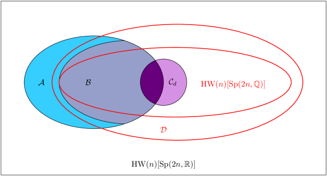
Figure 6: The classes of circuits considered in this work and previous works. The class $\mathcal{C}_{d}$ refers to the Clifford group for dimension $d$. Classes $\mathcal{A}$ and $\mathcal{B}$ are defined in Ref. [20] as the class of operations which are simulatable for single-mode and multi-mode measurement, respectively. $\mathcal{A},\mathcal{B},\mathcal{C}_{d}$ are all contained within the set of Gaussian operations $\text{HW}(n)[\text{Sp}(2n,\mathbb{R})]$. The class $\text{HW}(n)[\text{Sp}(2n,\mathbb{Q})]$ contains $\mathcal{C}_{d}$ but does not completely contain $\mathcal{A}$ nor $\mathcal{B}$. The class $\mathcal{D}$, as defined in this Appendix, contains $\mathcal{B},\mathcal{C}_{d}$ but is not known to contain $\mathcal{A}$. Note that the size of each of these regions in the diagram is arbitrary.

This class of operations $\text{HW}(n)[\text{Sp}(2n,\mathbb{Q})]$ contains, in particular, all GKP Clifford operations for encoded qudits of any dimension, as was proven in Sec. LABEL:sec:clifford.

We now recall and compare classes of operations that we demonstrated to be simulatable using different techniques in our previous work, Ref. [20], with those considered here. We previously demonstrated that circuits with input GKP states acted on by operations selected from a class $\mathcal{B}$ and measured in all modes with homodyne measurement are simulatable. This class was defined as

$$\mathcal{B}=\text{HW}(n)\times\text{DSp}(2n,\mathbb{R})$$ (156)

where

and

$$\Theta=\{\theta\in\mathbb{R}:\cot\theta=u/v\in\mathbb{Q}_{(2)}\}\cup\{0,\pi\}.$$ (157)

The class $\mathcal{B}$ contains operations where the symplectic matrix can contain irrational elements, e.g. when $\theta_{j}=\pi/4$, despite satisfying the condition that $\cot\theta_{j}\in\mathbb{Q}_{(2)}$. This implies that $\mathcal{B}\not\subset\text{HW}(n)\times\text{Sp}(2n,\mathbb{Q})$.

In Appendix C we demonstrated that it is possible to extend the class of simulatable operations beyond the group $\text{HW}(n)\times\text{Sp}(2n,\mathbb{Q})$, to a larger set which we denote $\mathcal{D}$ and we show that $\mathcal{B}\subset\mathcal{D}$. This set contains all displacements $\text{HW}(n)$ and all symplectic matrices such that $X^{T}X$ and $X^{T}Y$ are rational.

In our previous work [20] we demonstrated that is possible to simulate another class $\mathcal{A}$ which consists of symplectic operations whereby the top row of the symplectic matrix has a specific structure. That matrix does not necessarily satisfy any constraints in the other elements and so we cannot conclude that $\mathcal{D}$ nor $\text{HW}(n)\times\text{Sp}(2n,\mathbb{Q})$ contains $\mathcal{A}$.

We have included a figure, Fig. 6, to show the containment of each of these classes of operations, with respect to the previous classes identified in Ref. [20].

Appendix E Adaptive circuits with modular homodyne measurements

Although not required for the results of this paper, we provide an additional observation in this appendix. We demonstrate how to efficiently sample from a circuit that makes use of modular measurements. This method involves producing random integers selected from a finite set of integers.

Quantum circuits involving GKP states often make use of modular homodyne measurements. These are measurements in position or momentum modulo some period. Formally we define some period $T/\sqrt{\pi}\in\mathbb{Q}$ such that the recorded measurement result in position or momentum, $x_{1}$, is recorded as $x_{1}\mod T$. For example, Pauli $\hat{Z}$ measurements in the GKP framework [12] are measurements in position modulo $T=2\sqrt{\pi}$. If the measurement result $x_{1}$ is closest to $x_{1}\mod 2\sqrt{\pi}=0$, the measurement corresponds to a measurement of the logical qubit state $\ket{0}$. If the measurement result $x_{1}$ is closest to $x_{1}\mod 2\sqrt{\pi}=\sqrt{\pi}$, the measurement corresponds to a measurement of the logical qubit state $\ket{1}$.

An adaptive circuit with feed-forward operations that makes use of modular measurements will use the value of $x_{1}\mod 2\sqrt{\pi}$ to determine future operations. In the case of Pauli $\hat{Z}$ measurements, we can define two possible operations which could be performed on the remaining modes, depending on which outcome is measured.

The PDF of a unitary non-adaptive operation $U_{0}$ followed by a measurement of mode $1$ can be represented as

$$\text{PDF}(x_{1})= \sum_{\vec{m}\in\mathbb{Z}^{n}}\delta(x_{1}-\sqrt{\pi}\left((R^{T})^{-1}(\vec{t}+2\vec{m})\right)_{1}-c_{1})$$ (158)

which is equivalent to identifying that the possible measurement values of $x_{1}$ can be given by

$$x_{1}=\sqrt{\pi}\left(R^{-T}(\vec{t}+2\vec{m})\right)_{1}+c_{1}\quad\forall\quad\vec{m}\in\mathbb{Z}^{n}.$$ (159)

To identify the possible outcomes of $x_{1}\mod\sqrt{\pi}k$, we calculate

$$x_{1}\mod k\sqrt{\pi}=\sqrt{\pi}\left(R^{-T}(\vec{t}+2\vec{m})\right)_{1}+c_{1}\mod k\sqrt{\pi}.$$ (160)

The matrix $R$ is rational and so we can write [20]

$$((R^{-T})2\vec{m})_{1}=\frac{u}{v}m^{*}$$ (161)

which reduces the random vector of integers to a single integer $m^{*}\in\mathbb{Z}$, and a period $\frac{u}{v}\in\mathbb{Q}$, which depends on the first row of the matrix $R^{-T}$.

This allows us to simplify the possible measurement outcomes to

$$\bar{x}_{1}= x_{1}\mod k\sqrt{\pi}$$

$$= \sqrt{\pi}\left(R^{-T}\vec{t}\right)_{1}+\sqrt{\pi}\frac{u}{v}m^{*}+c_{1}\mod k\sqrt{\pi}$$ (162)

where we can restrict to at most $vk$ possible outcomes parameterized by $\bar{m}\in\{0,1,2,vk-1\}$, which each occur with equal probability. Simulation of measurement consists of choosing a random value of $\bar{m}$ from the finite set of possible integers.

Following the adaptive routine, we then choose a new operator $U_{1}(x_{1})$ dependent on the measured value of $x_{1}$ and simulate the circuit $U_{1}(x_{1})U_{0}$. This will provide us with points of the form

$$\text{PDF}(\vec{x})=\sum_{\vec{m}}\delta(x_{1}-\left(\sqrt{\pi}R^{\prime-T}(\vec{t}^{\prime}+2\vec{m}^{\prime})+\vec{c}^{\prime}\right)_{1})\dots\delta(x_{n}-\left(\sqrt{\pi}R^{\prime-T}(\vec{t}^{\prime}+2\vec{m}^{\prime})+\vec{c}^{\prime}\right)_{n}).$$ (163)

Choosing $x_{1}=\bar{x}_{1}$ and assuming no operations have been applied to the measured mode we have

$$\text{PDF}(\vec{x})=\sum_{\vec{m}}\delta(\frac{u}{v}\bar{m}-2\left(R^{\prime-T}\vec{m}^{\prime}\right)_{1})\dots\delta(x_{n}-\left(\sqrt{\pi}R^{\prime-T}(\vec{t}^{\prime}+2\vec{m}^{\prime})+\vec{c}^{\prime}\right)_{n}).$$ (164)

This expression can be simplified to a summation over $n-1$ integers.

References

- Chitambar and Gour [2019] E. Chitambar and G. Gour, Rev. Mod. Phys. 91, 025001 (2019).
- Gottesman [1997] D. Gottesman, PhD Thesis (1997), arXiv:quant-ph/9705052v1.
- Gottesman [1999] D. Gottesman, The Heisenberg representation of quantum computers, edited by S. P. Corney, R. Delbourgo, and P. D. Jarvis, Group22: Proceedings of the XXII International Colloquium on Group Theoretical Methods in Physics (Cambridge, MA, International Press, 1999) pp. 32–43, arXiv:quant-ph/9807006.
- Nielsen and Chuang [2000] M. A. Nielsen and I. L. Chuang, Quantum Computation and Quantum Information (Cambridge University Press, 2000).
- Bravyi and Kitaev [2005] S. Bravyi and A. Kitaev, Physical Review A 71, 022316 (2005).
- Reichardt [2005] B. W. Reichardt, Quantum Information Processing 4, 251 (2005).
- Bartlett et al. [2002] S. D. Bartlett, B. C. Sanders, S. L. Braunstein, and K. Nemoto, Phys. Rev. Lett. 88, 097904 (2002).
- Mari and Eisert [2012] A. Mari and J. Eisert, Physical Review Letters 109, 230503 (2012).
- Veitch et al. [2012] V. Veitch, C. Ferrie, D. Gross, and J. Emerson, New Journal of Physics 14, 113011 (2012).
- Albarelli et al. [2018] F. Albarelli, M. G. Genoni, M. G. A. Paris, and A. Ferraro, Physical Review A 98, 052350 (2018).
- Takagi and Zhuang [2018] R. Takagi and Q. Zhuang, Physical Review A 97, 062337 (2018).
- Gottesman et al. [2001] D. Gottesman, A. Kitaev, and J. Preskill, Physical Review A 64, 012310 (2001).
- Lloyd and Braunstein [1999] S. Lloyd and S. L. Braunstein, Phys. Rev. Lett. 82, 1784 (1999).
- Baragiola et al. [2019] B. Q. Baragiola, G. Pantaleoni, R. N. Alexander, A. Karanjai, and N. C. Menicucci, Phys. Rev. Lett. 123, 200502 (2019).
- Yamasaki et al. [2020] H. Yamasaki, T. Matsuura, and M. Koashi, Physical Review Research 2, 023270 (2020).
- de Beaudrap [2013] N. de Beaudrap, Quantum Information & Computation 13, 73 (2013), arXiv:1102.3354.
- Gheorghiu [2014] V. Gheorghiu, Physics Letters A 378, 505 (2014).
- Note [1] Note that in the main text, we simplify the class of simulatable operations to those which have a rational symplectic matrix. However, the class of simulatable operations also includes those given in the multimode case of Ref. [20]. We provide the broader requirements of the class of simulatable symplectic matrices in Appendix C.
- García-Álvarez et al. [2020] L. García-Álvarez, C. Calcluth, A. Ferraro, and G. Ferrini, Phys. Rev. Research 2, 043322 (2020).
- Calcluth et al. [2022] C. Calcluth, A. Ferraro, and G. Ferrini, arXiv:2203.11182 (2022).
- García-Álvarez et al. [2021] L. García-Álvarez, A. Ferraro, and G. Ferrini, in International Symposium on Mathematics, Quantum Theory, and Cryptography, edited by T. Takagi, M. Wakayama, K. Tanaka, N. Kunihiro, K. Kimoto, and Y. Ikematsu (Springer Singapore, Singapore, 2021) pp. 79–92.
- Rahimi-Keshari et al. [2016] S. Rahimi-Keshari, T. C. Ralph, and C. M. Caves, Physical Review X 6, 021039 (2016).
- Note [2] The Heisenberg-Weyl group is a normal subgroup of the semi-direct product of and , which we indicate by . Indeed, the subgroup is invariant under conjugation by any element of . Therefore, the full group of simulatable operations is specified by the semi-direct product of these two subgroups [54].
- Ferraro et al. [2005] A. Ferraro, S. Olivares, and M. G. A. Paris, Gaussian States in Quantum Information (Bibliopolis, Napoli, 2005) arXiv:quant-ph/0503237.
- Serafini [2017] A. Serafini, Quantum continuous variables : a primer of theoretical methods (CRC Press, Taylor & Francis Group, Boca Raton, FL, 2017).
- Kok and Lovett [2010] P. Kok and B. W. Lovett, Introduction to optical quantum information processing (Cambridge university press, 2010).
- Sakurai and Napolitano [2017] J. J. Sakurai and J. Napolitano, Modern Quantum Mechanics, 2nd ed. (Cambridge University Press, 2017).
- Gerry et al. [2005] C. Gerry, P. Knight, and P. L. Knight, Introductory quantum optics (Cambridge university press, 2005).
- Moore [1920] E. H. Moore, Bull. Am. Math. Soc. 26, 394 (1920).
- Penrose [1955] R. Penrose, in Mathematical proceedings of the Cambridge philosophical society, Vol. 51 (Cambridge University Press, 1955) pp. 406–413.
- Ben-Israel and Greville [2003] A. Ben-Israel and T. N. Greville, Generalized inverses: theory and applications, Vol. 15 (Springer Science & Business Media, 2003).
- Newman [1972] M. Newman, Integral Matrices, Pure and Applied Mathematics; a Series of Monographs and Textbooks No. v. 45 (Academic Press, 1972).
- Newman [1997] M. Newman, Linear algebra and its applications 254, 367 (1997).
- sta [2022a] Integer eigenvectors of a rational matrix (2022a), mathematics Stack Exchange. Available at https://math.stackexchange.com/questions/4391454/integer-eigenvectors-of-a-rational-matrix/4391951 (accessed: 2022-04-26).
- Note [3] Alternative previous results [55, 56] also exist for the simulation of CV circuits in the form of normalizer circuits. These results provide a numerical method to simulate non-adaptive normalizer circuits in the weak sense [36], i.e. it is possible to sample the output of a non-adaptive circuit. However, adaptivity is required for magic state distillation and so these results alone do not allow us to conclude that the vacuum is responsible for providing quantum advantage.
- Jozsa and Van Den Nest [2014] R. Jozsa and M. Van Den Nest, Quantum Information & Computation 14, 633 (2014).
- Arora and Barak [2009] S. Arora and B. Barak, Computational Complexity: A Modern Approach (Cambridge University Press, Cambridge, 2009).
- Mollin [2008] R. A. Mollin, Fundamental Number Theory with Applications, zeroth ed. (Chapman and Hall/CRC, 2008).
- Storjohann [2000] A. Storjohann, Dissertation, Swiss Federal Institute of Technology, Zurich (2000).
- Noh et al. [2022] K. Noh, C. Chamberland, and F. G. Brandão, PRX Quantum 3, 010315 (2022).
- Baragiola [2022] B. Q. Baragiola, private communication (2022).
- Note [4] Gaussian operations parameterized by irrational symplectic operations cannot in general be simulated with our method. We refer to our previous work [20] which demonstrates that when the symplectic matrix is irrational, the wavefunction of the transformed state corresponds to a periodic distribution which cannot be analytically reduced. Measuring in the position basis of a state which has been transformed by a general irrational symplectic matrix will have a PDF which will give random integer combinations of irrational numbers. Except for specific choices of irrational symplectic matrices, the measurement values will be randomly selected from a set dense on the real number line.
- Croom [2016] F. H. Croom, Principles of Topology, dover edition ed. (Dover Publications, Inc, Mineola, New York, 2016).
- sta [2022b] Is the symplectic group over the rationals dense on the symplectic group over the reals? (2022b), Mathematics Stack Exchange. Available at https://math.stackexchange.com/q/4510323/ (accessed: 2022-08-18).
- Artin [1988] E. Artin, Geometric Algebra, Wiley Classics Library (J. Wiley, New York, 1988).
- Weyl [1946] H. Weyl, The Classical Groups: Their Invariants and Representations, 2nd ed., Princeton Landmarks in Mathematics and Physics Mathematics (Princeton University Press, Princeton, N.J. Chichester, 1946).
- Pedoe [1988] D. Pedoe, Geometry, a Comprehensive Course (Dover Publications, New York, 1988).
- Trench [2003] W. F. Trench, Introduction to real analysis (Prentice Hall/Pearson Education, Upper Saddle River, N.J, 2003).
- Greub [1975] W. Greub, Linear Algebra, Graduate Texts in Mathematics, Vol. 23 (Springer, New York, 1975).
- Roman [2007] S. Roman, Advanced Linear Algebra, 3rd ed., Graduate Texts in Mathematics No. 135 (Springer, New York, 2007).
- Golub and Loan [1996] G. H. Golub and C. F. V. Loan, Matrix Computations, 3rd ed. (The John Hopkins University Press, 1996).
- Greville [1966] T. N. E. Greville, SIAM Review 8, 518 (1966).
- Arvind et al. [1995] Arvind, B. Dutta, N. Mukunda, and R. Simon, Pramana J. Phys. 45, 441 (1995).
- Dummit and Foote [1991] D. S. Dummit and R. M. Foote, Abstract algebra, Vol. 1999 (Prentice Hall Englewood Cliffs, NJ, 1991).
- Bermejo-Vega [2016] J. Bermejo-Vega, PhD Thesis, Technische Universität München Max-Planck-Institut für Quantenoptik (2016), arXiv:1611.09274.
- Bermejo-Vega et al. [2016] J. Bermejo-Vega, Y. Lin, and M. Van den Nest, Quantum Information and Computation 16, 0361 (2016).