celmech: A Python Package for Celestial Mechanics

Abstract

We present celmech, an open-source Python package designed to facilitate a wide variety of celestial mechanics calculations. The package allows users to formulate and integrate equations of motion incorporating user-specified terms from the classical disturbing function expansion of the interaction potential between pairs of planets. The code can be applied, for example, to isolate the contribution of particular resonances to a system’s dynamical evolution and develop simple analytical models with the minimum number of terms required to capture a particular dynamical phenomenon. Equations and expressions can be easily manipulated by leveraging the extensive symbolic mathematics capabilities of the sympy Python package. The celmech package is designed to interface seamlessly with the popular $N$-body code REBOUND to facilitate comparisons between calculation results and direct $N$-body integrations. The code is extensively documented and numerous example Jupyter notebooks illustrating its use are available online.

1 Introduction

Celestial mechanics is the oldest branch of physics and increasingly sophisticated analytical techniques for predicting planetary motions have been developed over the course of the subject’s long history. While precise orbital solutions are now typically found through direct numerical integrations of the equations of motion, analytic methods remain central to solving open problems in dynamics. We are often more interested in developing theoretical insight into the qualitative elements (e.g., mean motion resonances, secular evolution) responsible for dynamical phenomena such as chaos, transit timing variations, extreme orbital eccentricities etc. This is especially true when studying exoplanetary systems, where precise mass and orbital determinations are often unavailable, and analytical intuition can guide the construction and interpretation of suites of $N$-body integrations across a relevant subset of the vast parameter space.

The fact that planetary masses are much smaller than the central stellar mass, and that orbital eccentricities and inclinations are typically small, often makes it possible to model planetary dynamics using only a small number of slowly varying terms in the disturbing function expansion of the gravitational interaction potential between planet pairs (a Fourier series in the angular orbital elements and a power series in eccentricities and inclinations). Nevertheless, this long-standing approach can be tedious when formulating even relatively simple models as it entails identifying appropriate disturbing function terms, finding expressions for their coefficients, and then evaluating them by means of a variety of special functions. Examining any of the various high-order expansion disturbing function expansions published during the 19th century (e.g., Peirce, 1849; Le Verrier, 1855; Boquet, 1889), one quickly appreciates that formulating any sophisticated, high-order analytic theories by hand represents a monumental undertaking.

Since the sixties, such detailed work has been performed using specialized codes dedicated to computing and manipulating disturbing function expansions (see references in Henrard, 1989; Brumberg, 1995). The state-of-the-art TRIP code (Gastineau & Laskar, 2011, 2021), a dedicated computer algebra system for celestial mechanics, has proven especially valuable for studies the solar system’s long-term dynamics (Hoang et al., 2021, 2022; Mogavero & Laskar, 2022). However, such analyses have largely been limited to the specialized groups with the expertise to develop these highly technical routines.

By contrast, the last decade has clearly demonstrated the impact open-source scientific software can have on the field (Tollerud et al., 2019), both by opening up specialized calculations to a wide base of users, and by providing application programming interfaces (APIs) that enable the interconnection of separate codes in a broad range of new and creative ways. Particularly successful cases in the exoplanet field include, e.g., ttvfast (Deck et al., 2014), EXOFAST (Eastman et al., 2013), batman (Kreidberg, 2015), radvel (Fulton et al., 2018), REBOUND (Rein & Liu, 2012), REBOUNDx (Tamayo et al., 2020), exostriker (Trifonov, 2019), NbodyGradient (Agol et al., 2021), and exoplanet (Foreman-Mackey et al., 2021).

Ellis & Murray (2000) provided an important early step towards making computer-assisted disturbing function expansions more accessible to the wider research community. They derived a method for calculating coefficients associated with specific Fourier terms in the disturbing function. This offers an efficient alternative to computing complete high-order disturbing function expansions by means of dedicated computer algebra. Mathematica notebooks implementing their algorithm were made available as part of the online material accompanying the popular textbook Murray & Dermott (1999).

In this paper, we present celmech, an open-source Python package, which facilitates the manipulation of disturbing function expansions to any order in the eccentricities and inclinations, and enables a broad range of analytical investigations. celmech is built upon on the disturbing function expansion algorithm derived by Ellis & Murray (2000), though with important modifications described in Section 4 that allow the equations of motion to be formulated in a powerful Hamiltonian framework instead of in orbital elements. We have designed the code’s API to easily interface with the REBOUND package, streamlining comparisons between semi-analytic celmech models and direct $N$-body integrations. Additionally, celmech includes functionality for performing canonical transformations, which are useful for both extracting conserved quantities and reducing the dimensionality of various problems (Sec. 5.3). We also plan to incorporate additional modules in upcoming releases.

The plan of the paper is as follows: we present a simple example application in Section 2 with the goal of introducing readers to the code and illustrating a typical workflow before proceeding through more in-depth discussions of technical details in subsequent sections. Section 3 reviews the coordinate system and Hamiltonian framework that celmech uses to formulate the equations of motion. Section 4 describes celmech’s capabilities for performing disturbing function expansions in terms of both classical Keplerian orbital elements (Sec 4.1), as well as canonical variables (Sec 4.2). Section 5 introduces celmech’s object-oriented approach to modeling Hamiltonian systems in general (Sec. 5.1) as well as those specific to planetary systems (Sec. 5.2). It also describes celmech’s ability to manipulate Hamiltonian models via the application canonical transformations (Sec. 5.3), including Lie series transformation series that arise in Hamiltonian perturbation theory (Sec. 5.4). To aid the reader, we provide a list the main mathematical symbols appearing in the paper along with their definitions in Appendix A.

2 A Simple Example

We begin with a practical example to highlight some of the central machinery in celmech, demonstrate the code’s API, and illustrate a possible workflow. We consider a system of three Earth-mass planets around a solar-mass star. The inner two are initialized at the 3:2 mean-motion resonance (MMR) with orbital periods of $1$ and $1.5$ years respectively, while the third planet’s orbital period is 3.2 years and does not form any simple integer ratios with the inner two. The outermost orbit begins with zero eccentricity and inclination to the reference plane. The innermost orbit has both its eccentricity and inclination (in radians) set to 0.02, while the middle orbit has these quantities both set to 0.03. The longitudes of ascending node, and the pericenters of the inner two orbits lie along the positive $x$-axis, and both planets start at conjunction at their respective apocenters where their orbits are spaced furthest apart (Fig. 1). The accompanying Jupyter notebook shows how celmech conveniently interfaces with the REBOUND $N$-body package, which provides extensive functionality for initializing orbital configurations that can then be converted to a celmech PoincareHamiltonian object. The PoincareHamiltonian class, detailed below in Section 5.2, will be used throughout the present example to build and manipulate a Hamiltonian model for the system’s dynamics.

2.1 First-Order Approximation

The PoincareHamiltonian class has several functions for adding specific terms from the disturbing function between pairs of planets in a system that can be used build up a dynamical model. We expect that the 3:2 MMR between the inner two planets will be important, so we call the following method of our PoincareHamiltonian object, which we named Hp:

⬇

Hp.add_MMR_terms(p=3, q=1, indexIn=1, indexOut=2)

This adds the lowest order disturbing function terms in eccentricities and inclinations that are associated with a 3:2 MMR between planets 1 and 2 (the star has index 0) to the Hamiltonian represented by the PoincareHamiltonian object Hp. More generally, the arguments p and q are used to specify terms associated with any the $p:p-q$ resonance and the arguments indexIn and indexOut specify the pair of planets for which terms should be added.

We can check the terms added to the disturbing function terms by inspecting the Hp.df attribute, which prints them with their associated normalization in units of energy (this disambiguation is useful in systems with more than one pair of planets):

$$-\frac{Gm_{1}m_{2}}{a_{2,0}}\tilde{C}_{(3,-2,0,-1,0,0)}^{(0,0,0,0),(0,0)}(\alpha_{1,2})e_{2}\cos(3\lambda_{2}-2\lambda_{1}-\varpi_{2})-\frac{Gm_{1}m_{2}}{a_{2,0}}\tilde{C}_{(3,-2,-1,0,0,0)}^{(0,0,0,0),(0,0)}(\alpha_{1,2})e_{1}\cos(3\lambda_{2}-2\lambda_{1}-\varpi_{1})$$ (1)

At first order in eccentricities and inclinations there are only two disturbing function terms associated with the 3:2 MMR with the resonant angles $3\lambda_{2}-2\lambda_{1}-\varpi_{1}$ and $3\lambda_{2}-2\lambda_{1}-\varpi_{2}$. These terms would typically be found by hand, e.g., in the Appendix of Murray & Dermott (1999). In the notation of Murray & Dermott (1999), the expression would read

$$\mathrm{MD:} -\frac{Gm_{1}m_{2}}{a_{2,0}}\Bigg{[}f^{(3)}_{27}(\alpha_{1,2})e_{1}\cos(3\lambda_{2}-2\lambda_{1}-\varpi_{1})+f^{(3)}_{31}(\alpha_{1,2})e_{2}\cos(3\lambda_{2}-2\lambda_{1}-\varpi_{2})\Bigg{]}~{}.$$ (2)

Our $\tilde{C}$ coefficients correspond to the $f$ coefficients of Murray & Dermott (1999), where we choose to include some additional granularity in our $\tilde{C}$ indices for specifying higher order terms. The index convention is explained in the following subsection (Sec. 2.2).

The PoincareHamiltonian object also allows us to integrate the equations of motion using only the terms one has added to the disturbing function. We show the evolution for the middle planet’s orbital eccentricity in Fig. 1, comparing an $N$-body integration using REBOUND to our simple celmech model incorporating only the leading order resonant terms between the inner two planets.

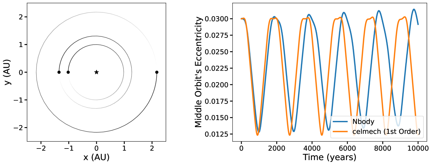
Figure 1: Left panel: Initial orbital configuration in the reference $x-y$ plane (inclinations to this plane are small $\lesssim 2^{\circ}$). Right panel: Comparison of the evolution of the middle planet’s orbital eccentricity between a celmech model including the leading-order 3:2 MMR terms in the disturbing function between the inner two planets (orange, Equation (1)) to an $N$-body integration (blue).

We see that the oscillation amplitude and frequency is reproduced to within $\approx 10\%$, though this causes the two models to quickly lose phase coherence. For many applications this level of agreement is sufficient, but we can improve the agreement by incorporating more terms at higher order in the eccentricities and inclinations.

2.2 Going to Second Order

Even going to just the next (second) order in the eccentricities and inclinations introduces a large number of additional terms. The disturbing function terms required to account for the 3:2 MMR interactions between the inner planet pair and the secular interactions between all planet pairs at second order in eccentricities and inclinations are given by

$$\begin{split}&-\frac{Gm_{1}m_{2}}{a_{2,0}}\tilde{C}_{(3,-2,0,-1,0,0)}^{(0,0,0,0)}(\alpha_{1,2})e_{2}\cos(3\lambda_{2}-2\lambda_{1}-\varpi_{2})-\frac{Gm_{1}m_{2}}{a_{2,0}}\tilde{C}_{(3,-2,-1,0,0,0)}^{(0,0,0,0)}(\alpha_{1,2})e_{1}\cos(3\lambda_{2}-2\lambda_{1}-\varpi_{1})\\ &-\frac{Gm_{1}m_{2}}{a_{2,0}}\tilde{C}_{(6,-4,0,-2,0,0)}^{(0,0,0,0)}(\alpha_{1,2})e_{2}^{2}\cos(6\lambda_{2}-4\lambda_{1}-2\varpi_{2})-\frac{Gm_{1}m_{2}}{a_{2,0}}\tilde{C}_{(6,-4,-1,-1,0,0)}^{(0,0,0,0)}(\alpha_{1,2})e_{1}e_{2}\cos(6\lambda_{2}-4\lambda_{1}-\varpi_{1}-\varpi_{2})\\ &-\frac{Gm_{1}m_{2}}{a_{2,0}}\tilde{C}_{(6,-4,-2,0,0,0)}^{(0,0,0,0)}(\alpha_{1,2})e_{1}^{2}\cos(6\lambda_{2}-4\lambda_{1}-2\varpi_{1})-\frac{Gm_{1}m_{2}}{a_{2,0}}\tilde{C}_{(6,-4,0,0,0,-2)}^{(0,0,0,0)}(\alpha_{1,2})i_{2}^{2}\cos(6\lambda_{2}-4\lambda_{1}-2\Omega_{2})\\ &-\frac{Gm_{1}m_{2}}{a_{2,0}}\tilde{C}_{(6,-4,0,0,-1,-1)}^{(0,0,0,0)}(\alpha_{1,2})i_{1}i_{2}\cos(6\lambda_{2}-4\lambda_{1}-\Omega_{1}-\Omega_{2})-\frac{Gm_{1}m_{2}}{a_{2,0}}\tilde{C}_{(6,-4,0,0,-2,0)}^{(0,0,0,0)}(\alpha_{1,2})i_{1}^{2}\cos(6\lambda_{2}-4\lambda_{1}-2\Omega_{1})\\ &-\frac{Gm_{1}m_{2}}{a_{2,0}}\tilde{C}_{(0,0,0,0,0,0)}^{(0,0,0,1)}(\alpha_{1,2})e_{2}^{2}-\frac{Gm_{1}m_{2}}{a_{2,0}}\tilde{C}_{(0,0,0,0,0,0)}^{(0,0,1,0)}(\alpha_{1,2})e_{1}^{2}-\frac{Gm_{1}m_{2}}{a_{2,0}}\tilde{C}_{(0,0,0,0,0,0)}^{(0,1,0,0)}(\alpha_{1,2})i_{2}^{2}-\frac{Gm_{1}m_{2}}{a_{2,0}}\tilde{C}_{(0,0,0,0,0,0)}^{(1,0,0,0)}(\alpha_{1,2})i_{1}^{2}\\ &-\frac{Gm_{1}m_{2}}{a_{2,0}}\tilde{C}_{(0,0,-1,1,0,0)}^{(0,0,0,0)}(\alpha_{1,2})e_{1}e_{2}\cos(-\varpi_{1}+\varpi_{2})-\frac{Gm_{1}m_{2}}{a_{2,0}}\tilde{C}_{(0,0,0,0,-1,1)}^{(0,0,0,0)}(\alpha_{1,2})i_{1}i_{2}\cos(-\Omega_{1}+\Omega_{2})\\ &-\frac{Gm_{1}m_{3}}{a_{3,0}}\tilde{C}_{(0,0,0,0,0,0)}^{(0,0,0,1)}(\alpha_{1,3})e_{3}^{2}-\frac{Gm_{1}m_{3}}{a_{3,0}}\tilde{C}_{(0,0,0,0,0,0)}^{(0,0,1,0)}(\alpha_{1,3})e_{1}^{2}-\frac{Gm_{1}m_{3}}{a_{3,0}}\tilde{C}_{(0,0,0,0,0,0)}^{(0,1,0,0)}(\alpha_{1,3})i_{3}^{2}-\frac{Gm_{1}m_{3}}{a_{3,0}}\tilde{C}_{(0,0,0,0,0,0)}^{(1,0,0,0)}(\alpha_{1,3})i_{1}^{2}\\ &-\frac{Gm_{1}m_{3}}{a_{3,0}}\tilde{C}_{(0,0,-1,1,0,0)}^{(0,0,0,0)}(\alpha_{1,3})e_{1}e_{3}\cos(-\varpi_{1}+\varpi_{3})-\frac{Gm_{1}m_{3}}{a_{3,0}}\tilde{C}_{(0,0,0,0,-1,1)}^{(0,0,0,0)}(\alpha_{1,3})i_{1}i_{3}\cos(-\Omega_{1}+\Omega_{3})\\ &-\frac{Gm_{2}m_{3}}{a_{3,0}}\tilde{C}_{(0,0,0,0,0,0)}^{(0,0,0,1)}(\alpha_{2,3})e_{3}^{2}-\frac{Gm_{2}m_{3}}{a_{3,0}}\tilde{C}_{(0,0,0,0,0,0)}^{(0,0,1,0)}(\alpha_{2,3})e_{2}^{2}-\frac{Gm_{2}m_{3}}{a_{3,0}}\tilde{C}_{(0,0,0,0,0,0)}^{(0,1,0,0)}(\alpha_{2,3})i_{3}^{2}-\frac{Gm_{2}m_{3}}{a_{3,0}}\tilde{C}_{(0,0,0,0,0,0)}^{(1,0,0,0)}(\alpha_{2,3})i_{2}^{2}\\ &-\frac{Gm_{2}m_{3}}{a_{3,0}}\tilde{C}_{(0,0,-1,1,0,0)}^{(0,0,0,0)}(\alpha_{2,3})e_{2}e_{3}\cos(-\varpi_{2}+\varpi_{3})-\frac{Gm_{2}m_{3}}{a_{3,0}}\tilde{C}_{(0,0,0,0,-1,1)}^{(0,0,0,0)}(\alpha_{2,3})i_{2}i_{3}\cos(-\Omega_{2}+\Omega_{3})~{}.\end{split}$$ (3)

We have gone from just two terms in Equation (1) to 26 terms in Equation (3). While the coefficients of such an expansion would be extremely tedious to look up by hand, these terms are easy to incorporate with celmech.

As can be verified in Equation (3), the $\tilde{C}$ subscript indices specify the coefficients of the cosine arguments

$$(k_{1},k_{2},k_{3},k_{4},k_{5},k_{6})\longleftrightarrow\cos(k_{1}\lambda_{out}+k_{2}\lambda_{in}+k_{3}\varpi_{in}+k_{4}\varpi_{out}+k_{5}\Omega_{in}+k_{6}\Omega_{out}),$$ (4)

where the “in” and “out” subscripts refer to the inner and outer body, respectively, and the ordering of the $k$ coefficients has been chosen to match the ordering conventionally used in the cosine arguments (e.g., Murray & Dermott, 1999). The amplitude of each cosine term is a power series in the eccentricities and inclinations. We choose to separate the terms in these expansions, and specify them by the $\tilde{C}$ superscript indices, as detailed in Sec. 4.2. Most terms in Equation (3) are the leading order contribution with superscripts $(0,0,0,0)$, though we see examples of higher order contributions in the secular terms without a cosine argument (all $k_{i}=0$ in Equation 4).

The most important second-order terms for our setup are the second-order 3:2 MMR terms, i.e., the 6:4 cosine terms above, involving the combination $6\lambda_{2}-4\lambda_{1}$. In celmech, we would incorporate MMR terms up to a specified maximum order by adding the max_order keyword to our call above:

⬇

Hp.add_MMR_terms(p=3, q=1, max_order=2, indexIn=1, indexOut=2)

The secular terms (terms above that do not depend on the mean longitudes $\lambda$, including those with no cosine factors) also make a small, but noticeable impact. For each pair of planet indices (idx1, idx2), the secular terms can be added by

⬇

Hp.add_secular_terms(max_order=2, indexIn=idx1, indexOut=idx2)

Comparing Fig. 1 with the left panel of Fig. 2, we see that this second-order model (orange curve) does improve the agreement with $N$-body.

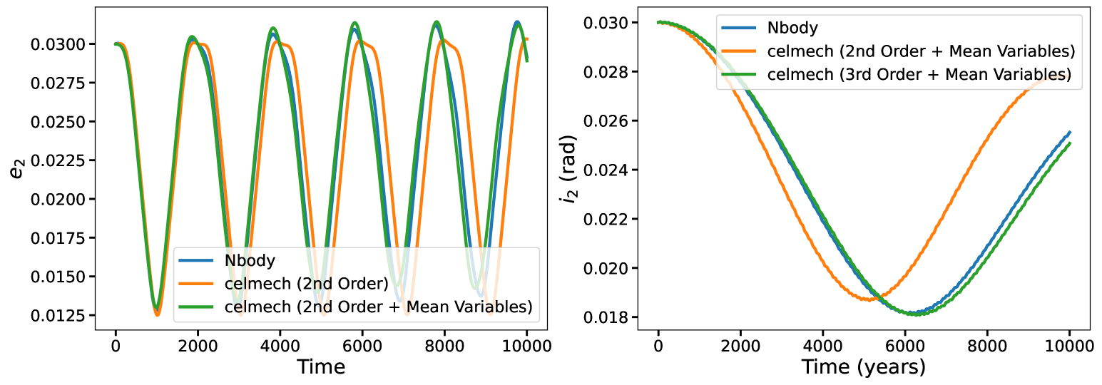
Figure 2: Left panel: Comparison of the evolution of the middle orbit’s eccentricity in our example between $N$-body (blue) and increasingly sophisticated celmech models. The orange curve incorporates the most important terms to second order in the eccentricities and inclinations, while the green curve additionally incorporates a correction from osculating to mean variables (see text). Right panel: Comparison of the evolution of the evolution of the middle orbit’s inclination between $N$-body (blue) and a second-order (orange) and third-order (green) celmech  model (both corrected to mean variables).

2.3 Mean Variables

While it is tempting to simply continue adding higher order terms, in this case it would not help. There is a separate issue causing a discrepancy with the $N$-body integrations, which can be fixed (at negligible computational cost) by converting from “osculating” to “mean” variables. Any time one takes only a subset of terms in the disturbing function, one is considering a (slightly) different problem from the full one. This distinction is particularly important, given our rather special initial conditions.

Each time an inner planet overtakes its outer neighbor at conjunction, it gains orbital energy on approach as it is being pulled forward by its outer neighbor, only to lose that energy approximately symmetrically on the way out. These encounters cause short-period “spikes” in the orbits’ semimajor axes, and the fact that we started our planets at conjunction, means that we are starting at the peak of one of those “spikes”. In other words, our initial semimajor axes are in a sense, spurious, and not reflective of the mean values they have over the vast majority of the orbit. This in turn impacts the period ratio between the inner two planets and their resonant dynamics.

Rather than incorporating even more terms in our disturbing function, the most elegant way of handling these (and other) ignored terms is through a near-identity canonical transformation from “osculating” to “mean” variables using Lie series (Morbidelli 2002, Sec. 5.4). One can do this in celmech by creating a FirstOrderGeneratingFunction object, and specifying the terms one wants to average out. The terms in the disturbing function causing the semimajor axis spikes discussed above are of the form $\cos\left[k(\lambda_{2}-\lambda_{1})\right]$, and can be analytically summed over (Malhotra 1993, Sec. 5.4). These terms are independent of the eccentricities and inclinations, and thus of zeroth-order, and can be added in celmech starting from a set of poincare_variables specifying the (osculating) initial conditions via

⬇

chi = FirstOrderGeneratingFunction(poincare_variables)

chi.add_zeroth_order_term()

The effects of unmodeled, nearby MMRs are much smaller for this problem than the zeroth-order terms above, but still make a noticeable difference, and are added by calls of the form

⬇

chi.add_MMR_terms(p=2,q=1,l_max=1, indexIn=1, indexOut=2)

chi.add_MMR_terms(p=4,q=1,l_max=1, indexIn=1, indexOut=2)

Once we have incorporated all the terms for which we want to correct, we transform to mean variables with chi.osculating_to_mean(), and the resulting integration (green curve in left panel of Fig. 2), yields excellent agreement with $N$-body.

2.4 Going to Higher Order

In the right panel of Fig. 2, we can see that, even at second-order (orange), there is a significant discrepancy with $N$-body (blue) in the orbital inclination evolution of the middle planet. In order to approach the $N$-body evolution, we have to include terms up to third order in the eccentricities and inclinations. This is the order at which terms directly coupling the inclinations to the quickly varying eccentricities first appear. These are easily obtained by setting max_order=3 in the calls above, though we spare the reader the details of the resulting 56 terms in the disturbing function. The add_secular_terms method accepts a similar max_order keyword argument, but higher order secular terms do not appear until 4th order in eccentricities and inclinations.

2.5 Limits

The degree of agreement between $N$-body and celmech models will depend on planet masses, with smaller masses generally giving better agreement. In particular, the conversion from “osculating” to “mean” variables is not perfect. The Lie series transformation (Sec. 5.4) corrects unmodeled terms (e.g., conjunctions, nearby MMRs) to first order in the planetary masses. This generates second-order (and higher) mass terms that should be added to the equations of motion governing the evolution of the “mean” variables. For our low-mass planets these corrections are negligible, but at higher mass-ratios with the central star, these terms start to be significant (Sansottera & Libert, 2019). Adding higher order terms in the eccentricities and inclinations will help until one reaches the level at which these second-order mass terms become significant.

2.6 Applications

Consideration of only the leading order terms is attractive for both analytical understanding and computational cost. As one incorporates more terms of progressively higher order, celmech can become slower than direct $N$-body integrations. Nevertheless, there are several applications for high-order models. First, in many instances it may be possible to deploy integration algorithms that are more efficient than celmech’s default general-purpose integrator and any such algorithms can potentially make use lower-level derivative and Jacobian information generated by the PoincareHamiltonian instance (i.e., Hp). This derivative and Jacobian information can also be valuable for locating equilibrium configurations such as periodic orbits via root-finding methods. High-order expansion can also be the starting point for developing accurate integrable approximations of the dynamics through canonical transformations (Hadden, 2019). Finally, incremental comparisons of successively higher order expansions with $N$-body integrations can also provide a quick guide to the degree of complexity required to model a particular dynamical phenomenon of interest.

3 Coordinate System

This section details the coordinate system and dynamical variables the celmech code uses for formulating Hamiltonian equations of motion. We begin by reviewing the Hamiltonian formulation of the planetary $N$-body problem, considering $N-1$ planets of mass $m_{i}$ with $i=1,...,N-1$ orbiting a central star of mass $M_{*}$. Let $\boldsymbol{u}_{*}$ and $\boldsymbol{u}_{i}$ be the Cartesian position vectors of the star and the planets, respectively, in the inertial barycentric frame. We start by formulating the Hamiltonian in term of canonical heliocentric coordinates, $(\boldsymbol{r}_{i},\tilde{\boldsymbol{r}}_{i})$, where $\boldsymbol{r}_{i}=\boldsymbol{u}_{i}-\boldsymbol{u}_{*}$ is the $i$th planet’s heliocentric position vector and $\tilde{\boldsymbol{r}}_{i}=m_{i}\dot{\boldsymbol{u}}_{i}$ is its canonically conjugate momentum (Laskar & Robutel, 1995). In these coordinates, the Hamiltonian reads

$$H = \sum_{i=1}^{N-1}H_{\mathrm{Kep},i}+\sum_{i=1}^{N-1}\sum_{j=1}^{i}H_{\mathrm{int.}}^{(i,j)}$$ (5)

where

$$H_{\mathrm{Kep},i} = \frac{1}{2}\frac{|\tilde{\boldsymbol{r}}_{i}|^{2}}{\mu_{i}}-\frac{GM_{i}\mu_{i}}{|\boldsymbol{r}_{i}|}$$ (6)

$$H_{\mathrm{int.}}^{(i,j)} = -\frac{Gm_{i}m_{j}}{|\boldsymbol{r}_{i}-\boldsymbol{r}_{j}|}+\frac{\tilde{\boldsymbol{r}}_{i}\cdot\tilde{\boldsymbol{r}}_{j}}{M_{*}}~{},$$ (7)

${\mu}_{i}=\frac{m_{i}M_{*}}{M_{*}+m_{i}}$, and ${M}_{i}={M_{*}+m_{i}}$.

We will perform a canonical transformation from the canonical heliocentric coordinates $(\boldsymbol{r}_{i},\tilde{\boldsymbol{r}}_{i})$ to the canonical modified Delaunay variables that constitute action-angle coordinates of the integrable two-body Hamilontians, $H_{\mathrm{Kep},i}$. In order to effect this transformation, we first define a set of ‘canonical heliocentric’ Keplerian orbital elements, $(a_{i},e_{i},I_{i},\lambda_{i},\varpi_{i},\Omega_{i})$, which represent, respectively, the planetary orbit’s semi-major axis, eccentricity, inclination, mean longitude, longitude of periapse, and longitude of ascending node. Standard orbital elements are computed from bodies’ three-dimensional Cartesian positions and velocities as well as a “gravitational parameter” (e.g., Murray & Dermott, 1999). For each planet, canonical heliocentric elements are computed from the Cartesian position vector $\boldsymbol{r}_{i}$, the “velocity” vector $\tilde{\boldsymbol{r}}_{i}/\mu_{i}$, and the gravitational parameter $GM_{i}$. While $\tilde{\boldsymbol{r}}_{i}/\mu_{i}$ does not correspond to any physical velocity vector in the system, this definition of canonical heliocentric elements ensures that the modified Delaunay variables, defined below, form a canonical set of action-angle coordinates for the two-body Hamiltonian, $H_{\mathrm{Kep},i}$. The celmech module nbody_simulation_utilities provides the function reb_calculate_orbits to compute canonical heliocentric orbital elements from a REBOUND simulation and the function reb_add_from_elements to add particles to a REBOUND simulation by specifying these elements (Jupyter Notebook example).

The canonical modified Delaunay coordinates are defined in terms of the canonical heliocentric orbital elements. The action variables are

$$\Lambda_{i} = \mu_{i}\sqrt{GM_{i}a_{i}}$$

$$\Gamma_{i} = \mu_{i}\sqrt{GM_{i}a_{i}}(1-\sqrt{1-e_{i}^{2}})$$

$$Q_{i} = 2\mu_{i}\sqrt{M_{i}a_{i}}\sqrt{1-e_{i}^{2}}\sin^{2}(I_{i}/2)$$ (8)

and have units of angular momentum. The angle variables canonically conjugate to the action variables $\Lambda_{i},\Gamma_{i},$ and $Q_{i}$ are $\lambda_{i}$, $\gamma_{i}=-\varpi_{i}$, and $q_{i}=-\Omega_{i}$, respectively. In order to avoid coordinate system singularities that leave the canonical variables $\gamma_{i}$ and $q_{i}$ undefined when $e_{i}=0$ and $I_{i}=0$, celmech formulates equations of motion in terms canonical coordinate-momentum pairs

$$(\eta_{i},\kappa_{i}) = \sqrt{2\Gamma_{i}}\times(\sin\gamma_{i},\cos\gamma_{i})$$

$$(\rho_{i},\sigma_{i}) = \sqrt{2Q_{i}}\times(\sin q_{i},\cos q_{i})$$ (9)

rather than $(\Gamma_{i},\gamma_{i})$ and $(Q_{i},q_{i})$. In modified Delaunay variables, the two-body Hamiltonian, Equation (6), simply becomes

$$H_{\mathrm{Kep},i}=\frac{G^{2}M_{i}^{2}\mu_{i}^{3}}{2\Lambda_{i}^{2}}~{}.$$ (10)

By contrast, $H_{\mathrm{int.}}^{(i,j)}$ does not admit a simple expression in terms of the canonical variables. Rather, the benefit of expressing the Hamiltonian in terms of classical action angle variables is that $H_{\mathrm{int.}}^{(i,j)}$ can be decomposed as a Fourier series in the canonical angle variables, enabling the application of methods of Hamiltonian perturbation theory.

4 Expansion of the Disturbing Function

The celmech.disturbing_function module provides tools for calculating coefficients appearing in the cosine series expansion of the interaction Hamiltonian, $H_{\mathrm{int.}}^{(i,j)}$ both in terms of both orbital elements as well as canonical variables. We begin by describing the expansion of the disturbing function in terms of orbital elements.

4.1 Expansion in Terms of Orbital Elements

In order to write the cosine series expansion, we will take $a_{j}>a_{i}$, define $\alpha=a_{i}/a_{j}$, $s_{i}=\sin(I_{i}/2)$, $\boldsymbol{\theta}_{i,j}=(\lambda_{j},\lambda_{i},-\gamma_{i},-\gamma_{j},-q_{i},-q_{j})$ and write

$$H^{(i,j)}_{\mathrm{int}}=-\frac{Gm_{i}m_{j}}{a_{j}}\sum_{\bf k}\sum_{\nu_{1},\nu_{2},\nu_{3},\nu_{4}=0}^{\infty}\tilde{C}_{\bf k}^{\boldsymbol{\nu}}(\alpha_{i,j})s_{i}^{|k_{5}|+2\nu_{1}}s_{j}^{|k_{6}|+2\nu_{2}}e_{i}^{|k_{3}|+2\nu_{3}}e_{j}^{|k_{4}|+2\nu_{4}}\cos({\bf k}\cdot\boldsymbol{\theta}_{i,j})$$ (11)

where ${\bf k}=(k_{1},k_{2},...k_{6})$ and $\boldsymbol{\nu}=(\nu_{1},...,\nu_{4})$ are integer multi-indices and $\alpha_{i,j}=a_{i}/a_{j}$. Rotation and reflection symmetries of the planets’ gravitational interactions dictate that $\tilde{C}^{\boldsymbol{\nu}}_{\bf k}(\alpha)\neq 0$ only if $\sum_{l=1}^{6}k_{l}=0$ and $k_{5}+k_{6}=2n$ where $n$ is an integer (e.g., Murray & Dermott, 1999). For small eccentricities and inclinations, the coefficient of the cosine term $\cos({\bf k}\cdot\boldsymbol{\theta}_{i,j})$ is of order $\sim s_{i}^{|k_{5}|}s_{j}^{|k_{6}|}e_{i}^{|k_{3}|}e_{j}^{|k_{4}|}$ and higher order corrections are of degree 2 and greater in the planets’ eccentricities and inclinations.

To compute the coefficients $\tilde{C}_{\bf k}^{\boldsymbol{\nu}}(\alpha)$ appearing in Equation (11), we first represent the interaction Hamiltonian as the sum of two parts, $H^{(i,j)}_{\mathrm{int}}=-\frac{Gm_{i}m_{j}}{a_{j}}({\cal R}^{(i,j)}_{\mathrm{dir.}}+{\cal R}^{(i,j)}_{\mathrm{ind.}})$ where we define the direct and indirect parts of the disturbing function as

$${\cal R}^{(i,j)}_{\mathrm{dir.}} = \frac{a_{j}}{|\boldsymbol{r}_{j}-\boldsymbol{r}_{i}|}$$

$$\mathrm{and}~{}{\cal R}^{(i,j)}_{\mathrm{ind.}} = -\frac{a_{j}}{GM_{*}m_{i}m_{j}}\tilde{\boldsymbol{r}}_{i}\cdot\tilde{\boldsymbol{r}}_{j}~{}$$ (12)

and we denote the contributions of ${\cal R}^{(i,j)}_{\mathrm{dir.}}$ and ${\cal R}^{(i,j)}_{\mathrm{ind.}}$ to the value of the coefficient $\tilde{C}_{\bf k}^{\boldsymbol{\nu}}(\alpha)$ as $[\tilde{C}_{\bf k}^{\boldsymbol{\nu}}(\alpha)]_{\mathrm{ind.}}$ and $[\tilde{C}_{\bf k}^{\boldsymbol{\nu}}(\alpha)]_{\mathrm{ind.}}$, respectively. Given values of $\bf{k}$ and $\boldsymbol{\nu}$, the celmech code implements the algorithm described in Ellis & Murray (2000) to compute $[\tilde{C}_{\bf k}^{\boldsymbol{\nu}}(\alpha)]_{\mathrm{dir.}}$ in terms of Laplace coefficients and their derivatives while the calculation of $[\tilde{C}_{\bf k}^{\boldsymbol{\nu}}(\alpha)]_{\mathrm{ind.}}$ is detailed in Appendix B. The celmech.disturbing_function module’s df_coefficient_Ctilde function can be used to compute the coefficients $\tilde{C}_{\bf k}^{\boldsymbol{\nu}}(\alpha)$. The function takes two integer tuples, $\textsf{k}=(k_{1},k_{2},...,k_{6})$ and $\textsf{nu}=(\nu_{1},...,\nu_{4})$, as arguments and returns a representation of the coefficient as a python dictionary with key-value pairs in the form $\{(p_{1},(j_{1},s_{1},n_{1})):A_{1},...,(p_{N},(j_{N},s_{N},n_{N})):A_{N},(\mathtt{{}^{\prime}indirect^{\prime}},p_{\mathrm{ind}}):A_{\mathrm{ind}}\}$ with

$$\tilde{C}_{\bf k}^{\boldsymbol{\nu}}(\alpha)=A_{\mathrm{ind}}\alpha^{-p_{\mathrm{ind}}/2}+\sum_{l=1}^{N}A_{l}\alpha^{p_{l}}\frac{d^{n_{l}}}{d\alpha^{n_{l}}}b_{s_{l}}^{(j_{l})}(\alpha)$$ (13)

where

$$b_{s}^{(j)}(\alpha)=\frac{1}{\pi}\int_{-\pi}^{\pi}\frac{\cos(j\theta)}{(1+\alpha^{2}-2\alpha\cos\theta)^{s}}d\theta~{},$$

$p_{l},n_{l},$ and $j_{l}$ are integers, and $s_{l}$ are half-integers.

The function celmech.disturbing_function module’s evaluate_df_coefficient_dict can be used to compute a numerical value of a coefficient, $\tilde{C}_{\bf k}^{\boldsymbol{\nu}}$, for a particular choice of $\alpha$. The function deriv_df_coefficient computes derivatives of disturbing function coefficients with respect to $\alpha$. This function takes a dictionary of the form returned by df_coefficient_Ctilde as an argument and returns a new dictionary of the same form representing the derivative of the coefficient with respect to $\alpha$. Some basic calculations of disturbing function coefficients are demonstrated in Jupyter example notebook DisturbingFunctionCoefficients.ipynb.

4.2 Expansion in Terms of Canonical Variables

While our $\tilde{C}_{\bf k}^{\boldsymbol{\nu}}$ coefficients for the direct part of the disturbing function match those of Ellis & Murray (2000) derived in terms of orbital elements, formulating Hamiltonian equations of motion requires a disturbing function expansion expressed in terms of canonical variables. To derive an expansion in terms of canonical variables we first introduce some auxillary variables: we introduce reference semi-major axes $a_{i,0}$ about which expansion of coefficients will be centered along with $\alpha_{ij,0}=a_{i,0}/a_{j,0}$, $\Lambda_{i,0}=\Lambda_{i}\sqrt{a_{i,0}/a_{i}}$ and $\delta_{i}=(\Lambda_{i}-\Lambda_{i,0})/\Lambda_{i,0}$. Next, we define $X_{i}=\sqrt{\frac{1}{\Lambda_{i,0}}}(\kappa_{i}-\mathrm{i}\eta_{i})$ and $Y_{i}=\frac{1}{2}\sqrt{\frac{1}{\Lambda_{i,0}}}(\sigma_{i}-\mathrm{i}\rho_{i})$, where we use a Roman ‘$\mathrm{i}$’ to denote the imaginary unit, i.e., $\mathrm{i}\equiv\sqrt{-1}$. The complex variables $z_{i}=e_{i}e^{\mathrm{i}\varpi_{i}}$ and $\zeta_{i}=s_{i}e^{\mathrm{i}\Omega_{i}}$ can then be expressed explicitly in terms of the variables $X_{i},Y_{i},$ and $\delta_{i}$ according to

$$z_{i} = \frac{1}{\sqrt{1+\delta_{i}}}X_{i}\sqrt{1-\frac{1}{4(1+\delta_{i})}X_{i}\bar{X}_{i}}$$ (14)

$$\zeta_{i} = \frac{1}{\sqrt{1+\delta_{i}}}\frac{Y_{i}}{\sqrt{1-\frac{1}{2(1+\delta_{i})}X_{i}\bar{X}_{i}}}~{}$$ (15)

where overlines denote complex conjugates. To express the amplitude of a single disturbing function cosine term, $\cos({\bf k}\cdot\boldsymbol{\theta}_{i,j})$, in terms of the canonical variables introduced in Section 3, we seek an expression for coefficients $C_{\bf k}^{\boldsymbol{\nu},\boldsymbol{l}}$ such that, when $k_{3},k_{4},k_{5},$ and $k_{6}>0$, the following relationship hold:

$$\left(\frac{1}{a_{j}}\right)z_{i}^{k_{3}}z_{j}^{k_{4}}\zeta_{i}^{k_{5}}\zeta_{j}^{k_{6}}\sum_{\boldsymbol{\nu}=0}^{\infty}\tilde{C}_{\bf k}^{\boldsymbol{\nu}}(\alpha_{ij})s_{i}^{2\nu_{1}}s_{j}^{2\nu_{2}}e_{i}^{2\nu_{3}}e_{j}^{2\nu_{4}}=\left(\frac{1}{a_{j,0}}\right)X_{i}^{k_{3}}X_{j}^{k_{4}}Y_{i}^{k_{5}}Y_{j}^{k_{6}}\sum_{\boldsymbol{l}=0}^{\infty}\sum_{\boldsymbol{\nu}=0}^{\infty}{C}_{\bf k}^{\boldsymbol{\nu},\boldsymbol{l}}(\alpha_{ij,0})|Y_{i}|^{2\nu_{1}}|Y_{j}|^{2\nu_{2}}|X_{i}|^{2\nu_{3}}|X_{j}|^{2\nu_{4}}\delta_{i}^{l_{1}}\delta_{j}^{l_{2}}~{}.$$ (16)

When $k_{3}<0$, $z_{i}^{k_{3}}$ and $X_{i}^{k_{3}}$ in Equation (16) are replaced with $\bar{z}_{i}^{-k_{3}}$ and $\bar{X}_{i}^{-k_{3}}$, respectively, and analogous substitutions for variables $(z_{j},\zeta_{i},\zeta_{j})$ and $(X_{j},Y_{i},Y_{j})$ are made when any of $k_{4},k_{5},$ or $k_{6}<0$. In Appendix C we work out explicit expressions for the coefficients ${C}_{\bf k}^{\boldsymbol{\nu},\boldsymbol{l}}$ in terms of terms of the $\tilde{C}_{\bf k}^{\boldsymbol{\nu}}$ coefficients and their derivatives. While these expressions are, in general, complicated, note that ${C}_{\bf k}^{(0,0,0,0),(0,0)}=\tilde{C}_{\bf k}^{(0,0,0,0)}$. The disturbing_function module’s df_coefficient_C function can be used to obtain disturbing function coefficients ${C}_{\bf k}^{\boldsymbol{\nu},\boldsymbol{l}}$.

4.3 Generating disturbing function arguments of a given order

In many applications, one is interested in gathering a series of particular disturbing function terms, such as those associated with a particular resonance, up to a maximum order, $N_{\mathrm{max}}$, in eccentricities and inclinations. The disturbing_function module provides the function df_arguments_dictionary that allows the user to enumerate all cosine arguments, ${\bf k}\cdot\boldsymbol{\theta}_{ij}$, appearing in the disturbing function expansion up to a given order $N_{\mathrm{max}}$ in inclinations and eccentricities. In order to do so, the function enumerates tuples $(k_{3},k_{4},k_{5},k_{6})$ that satisfy $|k_{3}|+|k_{4}|+|k_{5}|+|k_{6}|\leq N_{\mathrm{max}}$, along with the condition $k_{5}+k_{6}=2n$ for integer $n$. The latter condition ensures $C_{\bf k}^{\boldsymbol{n},\boldsymbol{l}}\neq 0$ (see Section 4.1). These terms are further grouped by their value of $\sum_{i=3}^{6}k_{i}$, which must be equal to $-(k_{1}+k_{2})$ to ensure $C_{\bf k}^{\boldsymbol{n},\boldsymbol{l}}\neq 0$. The Jupyter notebook example DisturbingFunctionArguments.ipynb illustrates how the results returned by df_arguments_dictionary are structured.

The disturbing_function module also provides the convenience function list_resonance_terms to create a list of all $\bf{k}$ and $\boldsymbol{\nu}$ combinations associated with a particular MMR that appear in the expansion of the disturbing function up to a user-specified order. In particular, given input $p$ and $q$ specifying the $p$:$p-q$ along with maximum order, list_resonance_terms returns a python list of tuples in the form $((k_{1},k_{2},...,k_{6}),(\nu_{1},...,\nu_{4}))$ that includes all terms that satisfy

$$(q-p)k_{1}+pk_{2}=0$$

$$|k_{3}|+|k_{4}|+|k_{5}|+|k_{6}|+2(\nu_{1}+\nu_{2}+\nu_{3}+\nu_{4})\leq N_{\mathrm{max}}$$ (17)

in addition to the usual rules $\sum_{i=1}^{6}k_{i}=0$ and $k_{5}+k_{6}=2n$ for integer $n$. Similarly, the function list_secular_terms can be used to create a list of all $\bf{k}$ and $\boldsymbol{\nu}$ combinations that appear as secular terms with $k_{1}=k_{2}=0$ in the disturbing function expansion up to a user-specified order. Both the list_resonance_terms and list_secular_terms functions are illustrated in a Jupyter notebook example.

4.4 Oblateness and General Relativity

The effects of primary oblateness and general relativistic precession can be important for the dynamical evolution of planetary systems. Here we give expressions for the orbit-averaged potentials of these effects in terms of the canonical variables used by celmech. The gravitational potential due to the quadrupole moment of an oblate central primary at a heliocentric position $\mathbf{r}$ is given by

$$\phi_{J_{2}}(\mathbf{r})=J_{2}\frac{GM_{*}R_{*}^{2}}{r^{3}}P_{2}(\hat{\mathbf{r}}\cdot\hat{\mathbf{z}})$$ (18)

where $r=|\mathbf{r}|$, $\hat{\mathbf{r}}=\mathbf{r}/r$, and $\hat{\mathbf{z}}$ is the direction perpendicular to the primary’s equatorial plane. In terms of orbital elements, $\hat{\mathbf{r}}\cdot\hat{\mathbf{z}}=\sin(I)\sin(f+\varpi-\Omega)=2s\sqrt{1-s^{2}}\sin(f+\varpi-\Omega)$ where $f$ is the true anomaly and the inclination, $I$, is measured relative to the primary’s equatorial plane. Denoting orbit-averaged values by $<\cdot>$, we use $<r^{-3}>=a^{-3}\left(1-e^{2}\right)^{-3/2}$ and $<r^{-3}\sin^{2}(f+\varpi-\Omega)>=\frac{1}{2}<r^{-3}>$ to find that the orbit-averaged value of the quadrupole potential is given by $<\phi_{J_{2}}>=-J_{2}\frac{GM_{*}}{a}\left(\frac{R_{*}}{a}\right)^{2}{\left(1-e^{2}\right)^{-3/2}}\left(1/2+{3(s^{4}-s^{2})}\right)$. The corresponding contribution to the Hamiltonian can be written in terms of canonical variables as

$$H_{J_{2}}(\Lambda,\eta,\kappa,\rho,\sigma) = -\frac{G^{4}M^{4}_{*}\mu^{6}J_{2}R_{*}^{2}}{\Lambda^{3}\left(\Lambda-\frac{1}{2}(\eta^{2}+\kappa^{2})\right)^{3}}\left[\frac{1}{2}-\frac{3}{4}\left(\frac{\rho^{2}+\sigma^{2}}{\Lambda-\frac{1}{2}(\eta^{2}+\kappa^{2})}\right)+\frac{3}{16}\left(\frac{\rho^{2}+\sigma^{2}}{\Lambda-\frac{1}{2}(\eta^{2}+\kappa^{2})}\right)^{2}\right]~{}.$$ (19)

Nobili & Roxburgh (1986) describe how the apsidal precession caused by general relativity (GR) can be approximated by including a potential term equal to

$$H_{\mathrm{GR}}(\eta,\kappa)=-\int_{-\pi}^{\pi}\frac{3G^{2}M_{*}^{2}}{c^{2}r^{2}}d\lambda=-\frac{3G^{2}M_{*}^{2}}{c^{2}a^{2}\sqrt{1-e^{2}}}=-\frac{3G^{4}M^{4}\mu^{4}}{\Lambda^{3}c^{2}\left(\Lambda-\frac{1}{2}\left(\eta^{2}+\kappa^{2}\right)\right)}~{}.$$ (20)

Primary oblateness and GR effects can be modeled by adding terms in the form of Equations (19) and (20) to the Hamiltonian represented by a PoincareHamiltonian object, described below in Section 5.2, using the add_orbit_average_J2_terms and add_gr_potential_terms methods.

5 Hamiltonian and Poincare Modules

This section begins in Section 5.1 with a description of how the celmech code represents general Hamiltonian systems. In Section 5.2, we describe the PoincareHamiltonian class, which is capable of representing the Hamiltonian of a planetary system by the inclusion of a collection of disturbing function terms capturing inter-planet gravitational interactions. Section 5.3 describes how canonical transformations, which can be applied to modify any Hamiltonian represented by celmech, are implemented. Section 5.4 describes the implementation of the FirstOrderGeneratingFunction class that can be used to apply techniques from canonical perturbation theory to “average” away fast oscillations in the instantaneous, “osculating” orbital elements and transform to “mean” elements that better track the system’s long-term evolution.

5.1 Representing Hamiltonian Systems

The celmech.hamiltonian module defines the PhaseSpaceState and Hamiltonian classes which serve as the basic objects used by celmech to represent Hamiltonian dynamical systems. The Jupyter example notebook SimplePendulum.ipynb provides a basic example that applies these classes to model the motion of a simple pendulum. PhaseSpaceState instances represent points in the phase space of a Hamiltonian dynamical system and store symbolic variables along with numerical values for canonical variables as key-value pairs of an ordered dictionary under the qp attribute. The Hamiltonian class can be used to define a Hamiltonian function of the phase space coordinates and momenta of a particular PhaseSpaceState instance. A Hamiltonian instance is initialized by passing a symbolic expression for the Hamiltonian along with a PhaseSpaceState instance. The PhaseSpaceState will then be stored by the new Hamiltonian object as its state attribute. The symbolic expression for the Hamiltonian should depend on the same canonical variables stored by the PhaseSpaceState instance. The Hamiltonian represented by a Hamiltonian class can also depend on any number of symbolic parameters whose numerical values should be set at initialization by passing a dictionary that pairs parameter symbols with their numerical values. Numerical parameter values are stored as the H_params attribute and can be updated at any point after initializing a Hamiltonian instance to explore how a system’s dynamics depends on parameter values.

In addition to storing a symbolic representation of the Hamiltonian function and its associated flow, a Hamiltonian object can be used to integrate the equations of motion and evolve a phase space trajectory in time. In order to do so, a Hamiltonian instance implements functions flow_func and jacobian_func that take numerical values of the canonical variables as input and return numerical value of the flow given by Hamilton’s equations, and its Jacobian with respect to the canonical variables. These function are used in conjunction with the scipy package’s (Virtanen et al., 2020) integrate.ode class to evolve the phase space state of the system.

5.2 Constructing Hamiltonians for Planetary Systems

The celmech.poincare module provides tools to model planetary systems’ dynamics by building a Hamiltonian from the disturbing function expansion described in Section 4. To build these Hamiltonian models, the module defines the Poincare class, a special subclass of the PhaseSpaceState class, and PoincareHamiltonian, a special subclass of the Hamiltonian class. The Poincare class represents the phase space state of an $N$-body planetary system in terms of the canonically conjugate coordinates $\boldsymbol{q}=(\lambda_{1},\eta_{1},\rho_{1},...,\lambda_{N-1},\eta_{N-1},\rho_{N-1})$ and momenta $\boldsymbol{p}=(\Lambda_{1},\kappa_{1},\sigma_{1},...,\Lambda_{N-1},\kappa_{N-1},\sigma_{N-1})$. In addition to storing these canonical variables, a Poincare instance owns a collection of PoincareParticle objects through the Poicare.particles attribute. The individual members of this collection represent the individual bodies of the $N$-body system, i.e., the star and planets. Each planet PoincareParticle object records the values of its mass and six canonical variables as well as various quantities, including orbital elements, derived from these values. The API for accessing the mass and orbital element values of individual PoincareParticle instances is designed to closely mirror that of the REBOUND particle class.

A PoincareHamiltonian is initialized by passing a Poincare object instance, which is then stored as the PoincareHamiltonian’s state attribute. Upon initialization, the symbolic Hamiltonian stored by a PoincareHamiltonian object for an $N$-body planetary system is simply the sum of $N-1$ individual Keplerian Hamiltonians. In other words, the Hamiltonian is given by $H=\sum_{i=1}^{N-1}H_{\mathrm{Kep},i}$ where $H_{\mathrm{Kep},i}$ is given by Equation (10). The user can then add specific interaction terms between pairs of planets from the disturbing function expansion described in Section 4 using a variety of methods of the PoincareHamiltonian class. The most basic method for adding disturbing function terms is PoincareHamiltonian.add_cosine_term. This method takes the integers $\mathbf{k}=(k_{1},...,k_{6})$ along with inner and outer planet indices, $i$ and $j$, as input and adds the terms

$$-\frac{Gm_{i}m_{j}}{a_{j,0}}\sum_{\boldsymbol{l},\boldsymbol{\nu}}C_{\bf{k}}^{\boldsymbol{\nu},\boldsymbol{l}}(\alpha_{i,j})|Y_{i}|^{|k_{5}|+2\nu_{1}}|Y_{j}|^{|k_{6}|+2\nu_{2}}|X_{i}|^{|k_{3}|+2\nu_{3}}|X_{j}|^{|k_{4}|+2\nu_{4}}\delta_{i}^{l_{i}}\delta_{j}^{l_{j}}\cos[{\bf k}\cdot\boldsymbol{\theta}_{ij}]~{}$$ (21)

to the Hamiltonian. The combinations of $\boldsymbol{l}$ and $\boldsymbol{\nu}$ occurring in the sum are controlled by the user through a variety of optional keyword arguments. If no keyword arguments are passed, the default behavior is to include only the lowest order contribution from the disturbing function, i.e., a single term with $\boldsymbol{l}=(0,0)$ and $\boldsymbol{\nu}=(0,0,0,0)$. The PoincareHamiltonian methods add_MMR_terms and add_secular_terms combine this basic add_cosine_term method with the functions for enumerating particular disturbing function arguments described in Section 4.3 to add collections of resonant or secular terms to the Hamiltonian up to a user-specified order in inclinations and eccentricities.

5.3 Canonical Transformations

The study of Hamiltonian systems is often greatly simplified by canonical transformations from one set of canonical variables to another that leave Hamilton’s equations unchanged. This allows for the algorithmic determination of constants of motion that can sometimes be used to greatly reduce the dimensionality of the problem (e.g., Hadden, 2019). The celmech CanonicalTransformation class provides a general framework for implementing canonical transformations. Instances of this class allow the user to apply canonical transformations to expressions by applying substitution rules that replace any occurrences old canonical variables with new ones and vice versa. A CanonicalTransformation instance can also be used to generate new Hamiltonian objects by applying its transformation to an existing Hamiltonian instance’s expression for the Hamiltonian, stored as the H attribute. The resulting Hamiltonian object’s state attribute will be a new PhaseSpaceState object representing the new canonical variables and its H attribute will be the transformed Hamiltonian.

Users can create canonical transformation objects by supplying sets of old and new canonical variables along with substitution rules. User’s can also use one the following class methods for initializing some frequently-used canonical transformations:

• from_type2_generating_function allows the user to specify a generating function $F_{2}(\boldsymbol{q},\boldsymbol{P})$ producing a canonical transformation that satisfies the equations

  $$\boldsymbol{Q}=\nabla_{\boldsymbol{P}}F_{2}~{} ;~{}\boldsymbol{p}=\nabla_{\boldsymbol{q}}F_{2}~{}.$$ (22)

  Provided an expression for the generating function, $F_{2}$, this method will attempt to automatically determine the corresponding transformation rules by applying sympy’s solve function to express the new variables $(\boldsymbol{Q},\boldsymbol{P})$ in terms of the old variables $(\boldsymbol{q},\boldsymbol{p})$ and vice versa.

• cartesian_to_polar produces a canonical transformation that transforms user-specified conjugate coordinate-momentum pairs of old variables $(q_{i},p_{i})$ to new conjugate pairs $(Q_{i},P_{i})=\left((\tan^{-1}(q_{i}/p_{i}),\frac{1}{2}(q_{i}^{2}+p_{i}^{2})\right)$. All other conjugate pairs will remain unchanged.

• polar_to_cartesian produces a canonical transformation that transforms user-specified conjugate pairs, $(q,_{i},p_{i})$, to new conjugate coordinate-momentum pairs $(Q_{i},P_{i})=\left(\sqrt{2p_{i}}\sin q_{i},\sqrt{2p_{i}}\cos q_{i}\right)$. All other conjugate pairs will remain unchanged.

• from_linear_angle_transformation produces the canonical transformation $(\boldsymbol{q},\boldsymbol{p})\rightarrow(\boldsymbol{Q},\boldsymbol{P})$ given by

  $$\boldsymbol{Q}=T\cdot\boldsymbol{q}~{} ;~{}\boldsymbol{P}=(T^{-1})^{\mathrm{T}}\cdot\boldsymbol{p}$$ (23)

  where $T$ is a user-supplied, invertible matrix.

• from_poincare_angles_matrix takes a Poincare instance as input, along with an invertible matrix $T$, and produces a transformation where the new canonical coordinates are linear combinations of the planets’ angular orbital elements given by $\boldsymbol{Q}=T\cdot(\lambda_{1},...,\lambda_{N},-\varpi_{1},...,-\varpi_{N}-\Omega_{1},...,-\Omega_{N})$ and the corresponding new conjugate momenta are given in terms of the canonical modified Delaunay variables described in Section 3 by $\boldsymbol{P}=(T^{-1})^{\mathrm{T}}\cdot(\Lambda_{1},...,\Lambda_{N},\Gamma_{1},...,\Gamma_{N},Q_{1},...,Q_{N})$.

• Lambdas_to_delta_Lambdas takes a Poincare instance as input and implements the canonical transformation replacing the $\Lambda_{i}$ variables with $\delta\Lambda_{i}=\Lambda_{i}-\Lambda_{i,0}$ as the momenta canonically conjugate to planets’ mean longitudes, $\lambda_{i}$.

• rescale_transformation produces a canonical transformation that simultaneously rescales the Hamiltonian and all canonical momentum variables by a common factor, $f$. In other words, if $H$ is the old Hamiltonian and $p_{i}$ are the old momentum variables, the new Hamiltonian will be $H^{\prime}=fH$ and $p_{i}^{\prime}=fp_{i}$ will replace $p_{i}$ as momentum variables conjugate to the old coordinates $q_{i}$. The user can optionally specify a subset of canonical variable pairs $(y_{i},x_{i})$ as Cartesian pairs which will be transformed so that the new, re-scaled variables are instead $(y^{\prime}_{i},x^{\prime}_{i})=(\sqrt{f}y_{i},\sqrt{f}x_{i})$.

• composite combines a series of canonical transformations.

While time-dependent canonical transformations are not currently supported, they can always be implemented by re-formulating the Hamiltonian under consideration in the extended phase space that includes time and the negative of the system’s energy as an additional conjugate variable pair.

Often a canonical transformations are applied to eliminate the explicit dependence of the transformed Hamiltonian on one or more canonical variables. This is because, when the transformed Hamiltonian does not depend on one of the angle variables, its the corresponding conjugate momentum variable is conserved and Hamilton’s equations for the remaining degrees of freedom are simplified. To make the discussion more concrete, suppose we have a canonical transformation of the canonical variables of an $N$ degree of freedom system $(q_{i},p_{i})\rightarrow(\phi_{1},...,\phi_{M},Q_{1},....,Q_{N-M},I_{1},...,I_{M},P_{1},...,P_{N-M})$ where the transformed Hamiltonian, $H^{\prime}(Q_{i},P_{i};I_{j})$, is independent of the coordinate variables $\phi_{j}$. so that the quantities $I_{1},...,I_{M}$ are constant. When such an elimination can be accomplished, it is frequently convenient to consider a system’s dynamics in the reduced phase space comprised of the remaining $N-M$ degrees of freedom with canonical variables $(Q_{i},P_{i})$ and treat the $M$ conserved quantities, $I_{j}$, as parameters of the Hamiltonian. When transforming a Hamiltonian by applying the old_to_new_hamiltonian method of a CanonicalTransformation object, the user has the option to automatically detect whether the resulting transformed Hamiltonian is independent of any of the new canonical variables and, if so, produce a Hamiltonian object with a state attribute respresenting a point in the reduced phase space with canonical variables $(Q_{i},P_{i})$ and with the quantities $I_{j}$ stored as parameters under the Hamiltonian object’s H_params attribute. To enable the application of the inverse transformation from the new canonical variables back to old ones in this situation, the new Hamiltonian object possess a full_qp attribute that stores the full set of variables, $(\phi_{1},...,\phi_{M},Q_{1},....,Q_{N-M},I_{1},...,I_{M},P_{1},...,P_{N-M})$, while the qp attribute only stores the variables of the reduced phase space, $(Q_{i},P_{i})$. The reduced Hamiltonian object’s full_qp attribute will only store the initial values of the ignorable coordinates, $\phi_{j}$, determined at the time the transformation was applied. It is important to recognize the the actual time evolution of these coordinates, given by $\frac{d}{dt}\phi_{j}=\frac{\partial}{\partial I_{j}}H^{\prime}(Q_{i},P_{i};I_{j})$, is generally non-trivial and depends on the specific trajectory, $(Q_{i}(t),P_{i}(t))$, of the system in the reduced phase space. Consequently, it will usually not be possible to re-construct the full phase space state of the system in the old canonical variables $(q_{i},p_{i})$ if only the reduced equations of motion governing the $(Q_{i},P_{i})$ are integrated. Nonetheless, in many applications the values of these ignorable coordinates are unimportant for the aspects the dynamics one wishes to study and application of the inverse transformation to the data stored in the full_qp attribute can provide useful information about how the system evolves in the original canonical variables. A basic illustration of these principles is provided in an example Jupyter notebook.

5.4 Lie series transformations

Modeling the dynamics of a planetary system with a Hamiltonian that includes only a finite number of terms from a disturbing function can be justified because the infinite number of ignored terms are rapidly oscillating and have negligible average influence on the motion, at least over sufficiently short timescales. Nevertheless, these fast oscillations in the full problem can make it challenging to match initial conditions in an “averaged” formulation, and such discrepancies can make comparisons between analytical and $N$-body models challenging, especially near regions of phase space where the dynamical behavior changes sharply, e.g., near resonance boundaries. Additionally, while typically we are interested in methods for removing these nuisance terms in the disturbing function, there are also cases where these fast oscillations are of primary interest. An important example is for transiting pairs of planets near (but not in) mean motion resonances, where the “fast” oscillations due to the resonant terms are observable as transit timing variations (for a Lie sires approach to TTVs, see Nesvorný & Morbidelli, 2008).

A powerful approach for transforming back and forth between instantaneous, or “osculating”, canonical variables (which are subject to a multitude of fast oscillations) and “mean” variables that remove these fast modes, is through the Lie series method. This technique introduces a near-identity canonical transformation (ensuring that the “mean” variables remain canonical) that, by construction, can cancel any set of rapidly oscillating terms in the Hamiltonian to first order in the planet-star mass ratio. This transformation is often referred to as “averaging” since, at this leading order in the masses, the technique is equivalent to averaging the problem over the rapidly oscillating angles. An advantage of the Lie series method is that it explicitly constructs the resultant terms at higher orders in the masses, which are not available through an averaging approach. A thorough discussion of canonical perturbation theory using the Lie series method, including important issues related to chaos, non-integrability, and the (non-)convergence of these series, is beyond the scope of this paper and can be found in references such as Morbidelli (2002) or Lichtenberg & Lieberman (2013). We will limit our discussion to the construction of canonical transformations to first order in the planet-star mass ratios, which are equivalent to transformations back and forth between osculating and mean variables, and are implemented in celmech.

To introduce Lie-series generating functions, consider splitting the Hamiltonian of a $N$-body system into three pieces: a Keplerian piece given by $H_{\mathrm{Kep}}=\sum_{i=1}^{N-1}H_{\mathrm{Kep},i}$, a term $H_{\mathrm{slow}}$ contains slowly varying disturbing function terms such as those with (near) resonant cosine arguments or secular terms, and a term $H_{\mathrm{osc}}$ that contains rapidly oscillating with negligible influence on the dynamics. We seek a canonical transformation that eliminates $H_{\mathrm{osc}}$ to first order in planet masses. In other words, we seek a canonical transformation $T:({\bf q},{\bf p})\rightarrow({\bf q^{\prime}},{\bf p^{\prime}})$ such that the transformed Hamiltonian is $H^{\prime}\equiv H\circ T^{-1}=H_{\mathrm{Kep}}+H_{\mathrm{slow}}+\mathcal{O}((m/M_{*})^{2})$. We use the Lie series method to construct such a transformation. The Lie transformation, $\exp[\mathcal{L}_{\chi}]$, of a function of phase space coordinates, $f$, is defined in terms of the Lie derivative operator, $\mathcal{L}_{\chi}\equiv[\cdot,\chi]$, as

$$\exp[\mathcal{L}_{\chi}]f=\sum_{n=0}^{\infty}\frac{1}{n!}\mathcal{L}_{\chi}^{n}f=f+[f,\chi]+\frac{1}{2}[[f,\chi],\chi]+...~{}.$$ (24)

Since a Lie transformation evolves $f$ under the flow induced by Hamilton’s equations for the “Hamiltonian” $\chi$ it is canonical by construction. The Lie series method seeks to find a generating function $\chi$ such that the Lie transformation $\exp[\mathcal{L}_{\chi}]$ produces the desired transformation, $T$, that eliminates the unwanted terms. If the generating function, $\chi$, is itself of order $\mathcal{O}(m/M_{*})$ then the transformed Hamiltonian is $H^{\prime}=\exp[\mathcal{L}_{\chi}]H\approx H_{\mathrm{Kep}}+H_{\mathrm{slow}}+H_{\mathrm{osc}}+[H_{\mathrm{Kep}},\chi]$ after dropping terms $\mathcal{O}((m/M_{*})^{2})$ and the generating function $\chi$ should satisfy $[H_{\mathrm{Kep}},\chi]=-H_{\mathrm{osc}}$. Noting that the Poisson bracket of $H_{\mathrm{Kep}}$ with all canonical variables except the mean longitudes vanishes and that

$$\left[H_{\mathrm{Kep}},\frac{\sin(\mathbf{k}\cdot{\boldsymbol{\theta}_{i,j}})}{k_{1}n_{j}+k_{2}n_{i}}\right]=-\cos(\mathbf{k}\cdot{\boldsymbol{\theta}_{i,j}})$$ (25)

where $n_{i}=\partial H_{\mathrm{Kep}}/\partial\Lambda_{i}$ is the $i$th planet’s mean motion, we immediately see that any disturbing function terms in $H_{\mathrm{osc}}$ involving planets $i$ and $j$ written in the form of Equation (21) will be eliminated to first order in the planet masses by simply including a corresponding term in $\chi$ that replaces $\cos(\mathbf{k}\cdot{\boldsymbol{\theta}_{i,j}})$ with ${\sin(\mathbf{k}\cdot{\boldsymbol{\theta}_{i,j}})}/({k_{1}n_{j}+k_{2}n_{i}})$ provided $k_{1}n_{j}+k_{2}n_{i}\neq 0$. The condition that $k_{1}n_{j}+k_{2}n_{i}\neq 0$ should always be satisfied since $H_{\mathrm{osc}}$ is presumed to be comprised only of rapidly oscillating terms.

The celmech class FirstOrderGeneratingFunction allows users to construct a generating function $\chi$ that eliminates a user-specified collection of disturbing function terms in the transformed Hamiltonian to first order in planet masses following the approach just described above. Terms are added to the generating function in much the same way that terms are added to a PoincareHamiltonian instance. In fact, FirstOrderGeneratingFunction is a subclass of the PoincareHamiltonian of PoincareHamiltonian that overwrites the parent class’s routines for adding cosine terms so that the trigonometric terms $\cos(\mathbf{k}\cdot{\boldsymbol{\theta}_{i,j}})$ are instead replaced with ${\sin(\mathbf{k}\cdot{\boldsymbol{\theta}_{i,j}})}/({k_{1}n_{j}+k_{2}n_{i}})$. The class provides a symbolic representations of the generating function under the chi and N_chi attributes, similar to the PoincareHamiltonian class’s H and N_H attributes. The class also provides an array of methods for transforming canonical variables and deriving perturbative solutions to the equations of motion. These are demonstrated in example notebooks here and here.

In addition to term-wise elimination of individual rapidly oscillating disturbing function terms described above, It is possible to remove all harmonics depending solely on the angular combination $\psi=\lambda_{i}-\lambda_{j}$ to zeroth order in eccentricities and inclinations with a single transformation. A number of authors have previously exploited the fact that perturbative solutions for planets’ mutual perturbation at zeroth order in eccentricities and inclinations can be expressed in closed form without needing to resort to an expansion in Fourier harmonics (e.g., Malhotra, 1993; Agol et al., 2005; Nesvorný & Vokrouhlický, 2014; Hadden et al., 2019), though not all these studies deploy a Lie series formalism. To zeroth order in inclinations and eccentricities, the disturbing function, ${\cal R}^{(i,j)}_{\mathrm{dir.}}+{\cal R}^{(i,j)}_{\mathrm{ind.}}$, given in Equation (12) can be written as

$${\cal R}^{(i,j)}_{\mathrm{dir.}}+{\cal R}^{(i,j)}_{\mathrm{ind.}}\approx P(\lambda_{j}-\lambda_{i};\alpha)-\frac{1}{\sqrt{\alpha}}\cos(\lambda_{i}-\lambda_{j})+\mathcal{O}(e,I^{2})$$ (26)

where $P(\psi;\alpha)=(1+\alpha^{2}-2\alpha\cos(\lambda_{j}-\lambda_{i}))^{-1/2}$. Therefore, a Lie series transformation with generating function

$$\chi = -\frac{Gm_{1}m_{2}}{a_{2}(n_{1}-n_{2})}\left(-\frac{1}{\sqrt{\alpha}}\sin({\lambda_{i}-\lambda_{j}})+\int^{\lambda_{i}-\lambda_{j}}_{0}\left(P(\psi,\alpha)-\bar{P}(\alpha)\right)d\psi\right)~{},$$ (27)

where $\bar{P}(\alpha)=\frac{1}{2\pi}\int_{-\pi}^{\pi}P(\psi,\alpha)d\psi$ is the mean value of $P(\psi,\alpha)$, will eliminate the disturbing function terms in Equation (26). The integral in Equation (27) can be written explicitly in terms of elliptic integrals as

$$\int^{\psi}_{0}\left(P(\psi^{\prime},\alpha)-\bar{P}(\alpha)\right)d\psi^{\prime}=\frac{2}{1-\alpha}F\left(\frac{\psi}{2}\bigg{|}-\frac{4\alpha}{(1-\alpha)^{2}}\right)-\frac{2}{\pi}\mathbb{K}(\alpha^{2})\psi$$ (28)

where $\mathbb{K}$ is the complete elliptic integral of the first kind and $F(\cdot|m)$ is an incomplete elliptic integrals of the first kind with modulus $m$. A term of the form given in Eqauation (27) can be added to the symbolic generating function stored by a FirstOrderGeneratingFunction object with the add_zeroth_order_term method.

6 Summary

In this paper we presented celmech, an open-source python package for conducting celestial mechanics calculations. The code combines a disturbing function expansion algorithm based on a method originally devised Ellis & Murray (2000) with the symbolic mathematics capabilities provided by the sympy library (Meurer et al., 2017) to enable users to efficiently create and integrate Hamiltonian models for planetary systems. The celmech API is designed so that users can easily compare these Hamiltonian models to direct $N$-body integrations with the REBOUND code (Rein & Liu, 2012).

The code is available through the Python Package Index (PyPI) as well as on GitHub at github.com/shadden/celmech. The code can can be freely redistributed under the GPL-3.0 license. Online documentation can be found at celmech.readthedocs.io. A library of Jupyter notebook examples illustrating various features and applications of the code is available at github.com/shadden/celmech/tree/master/jupyter_examples.

The celmech code’s modular design will allow ongoing development. Some features currently implemented in celmech, in addition to the modules and capabilities detailed in this paper, include tools for formulating and integrating equations of motion governing MMRs that are derived from numerically averaged disturbing functions (rather than truncated power series expansions in eccentricity and inclination) and tools for formulating and integrating secular equations of motion. We plan to detail additional features in forthcoming papers.

Appendix A Table of Symbols

Table 1 lists the main mathematical symbols used in the text along with brief descriptions as appropriate.

Table 1: Summary of mathematical notation used throughout the paper. We include short definitions and/or references to equations where quantities are defined when appropriate.

Name	Expression	Description
$G$		Newton’s gravitational constant
$M_{*}$		Mass of central star
$m_{i}$		Mass of $i$th planet
$\boldsymbol{r}_{i}$		Heliocentric position of $i$th planet
$\tilde{\boldsymbol{r}}_{i}$		Barycentric momentum of $i$th planet
$a_{i}$		Semi-major axis of $i$th planet
$e_{i}$		Eccentricity of $i$th planet
$I_{i}$		Inclination of $i$th planet
$\lambda_{i}$		Mean longitude of $i$th planet
$\varpi_{i}$		Longitude of periapse $i$th planet
$\Omega_{i}$		Longitude of ascending node $i$th planet
$s_{i}$	$\sin(I_{i}/2)$	Inclination variable appearing in many classic disturbing function expansions
$\mu_{i}$	$m_{i}M_{*}/(M_{*}+m_{i})$	Reduced mass of $i$th planet
$M_{i}$	$M_{*}+m_{i}$	Effective central mass for $i$th planet’s orbit
$\Lambda_{i}$	$\mu_{i}\sqrt{GM_{i}a_{i}}$	Canonical momentum conjugate to $\lambda_{i}$
$\Gamma_{i}$	$\Lambda_{i}(1-\sqrt{1-e_{i}^{2}})$	Canonical momentum conjugate to $\gamma_{i}=-\varpi_{i}$
$Q_{i}$	$=2\Lambda_{i}\sqrt{1-e_{i}^{2}}\sin^{2}(I_{i}/2)$	Canonical momentum conjugate to $q_{i}=-\Omega_{i}$
$\kappa_{i}$	$=\sqrt{2\Gamma_{i}}\cos{\varpi_{i}}$
$\eta_{i}$	$=-\sqrt{2\Gamma_{i}}\sin{\varpi_{i}}$
$\sigma_{i}$	$=\sqrt{2Q_{i}}\cos{\Omega_{i}}$
$\rho_{i}$	$=-\sqrt{2Q_{i}}\sin{\Omega_{i}}$
$\mathcal{R}^{(i,j)}_{\mathrm{dir.}}$	$=\frac{a_{j}}{|\mathbf{r}_{j}-\mathbf{r}_{i}|}$	Direct component of disturbing function
$\mathcal{R}^{(i,j)}_{\mathrm{ind.}}$	$=\frac{a_{j}}{GM_{*}m_{j}m_{i}}\tilde{\mathbf{r}}_{j}\cdot\tilde{\mathbf{r}}_{i}$	Indirect component of disturbing function
$\alpha_{i,j}$	$=a_{i}/a_{j}$	Semi-major axis ratio
$\boldsymbol{\theta}_{i,j}$	$=(\lambda_{j},\lambda_{i},\varpi_{i},\varpi_{j},\Omega_{i},\Omega_{j})$	Vector of angle variables
$\tilde{C}_{\bf k}^{\boldsymbol{\nu}}(\alpha)$		Disturbing function coefficient of $\cos(\boldsymbol{k}\cdot\boldsymbol{\theta}_{i,j})$ for expansion in $e_{i}$ and $s_{i}$
$b_{s}^{(s)}(\alpha)$	$\frac{1}{\pi}\int_{-\pi}^{\pi}\frac{\cos(j\theta)}{(1+\alpha^{2}-2\alpha\cos\theta)^{s}}$	Laplace coefficient
$z_{i}$	$=e_{i}\exp(\mathrm{i}\varpi_{i})$	Complex eccentricity
$\zeta_{i}$	$=s_{i}\exp(\mathrm{i}\Omega_{i})$	Complex inclination variable
$\Lambda_{i,0}$		Reference value for $\Lambda_{i}$
$\delta_{i}$	$\Lambda_{i}/\Lambda_{i,0}-1$	Fractional deviation of $\Lambda_{i}$ from reference value $\Lambda_{i,0}$
$X_{i}$	$=\sqrt{\frac{1}{\Lambda_{i,0}}}(\kappa_{i}-\mathrm{i}\eta_{i})$	$\approx e_{i}\exp(\mathrm{i}\varpi_{i})+\mathcal{O}(e_{i}^{3})$
$Y_{i}$	$=\sqrt{\frac{1}{4\Lambda_{i,0}}}(\sigma_{i}-\mathrm{i}\rho_{i})$	$\approx\sin(I_{i}/2)\exp(\mathrm{i}\Omega_{i})+\mathcal{O}(I_{i}e_{i}^{2})$
${C}_{\bf k,\boldsymbol{l}}^{\boldsymbol{\nu}}(\alpha)$		Disturbing function coefficient of $\cos(\boldsymbol{k}\cdot\boldsymbol{\theta}_{i,j})$ for expansion in $X_{i}$,$Y_{i}$, and $\delta_{i}$

Appendix B Expansion of the Indirect Disturbing Function

In this appendix we detail the expansion of the indirect component of the disturbing function,

$${\cal R}^{(i,j)}_{\mathrm{ind.}}=-\frac{a_{j}}{GM_{*}m_{i}m_{j}}\tilde{\boldsymbol{r}}_{i}\cdot\tilde{\boldsymbol{r}}_{j}~{},$$

closely following Laskar & Robutel (1995), who present a method for deriving a complete expansion of the indirect disturbing function, best accomplished with the aid of computer algebra. We extend their derivation in order to provide explicit formulas for disturbing function coefficients associated with specific cosine arguments. Writing $\tilde{\boldsymbol{r}}_{i}=\mu_{i}n_{i}a_{i}{\boldsymbol{v}}_{i}$, the indirect disturbing function can be written as

$${\cal R}^{(i,j)}_{\mathrm{ind.}}=-\frac{n_{i}n_{j}a_{j}^{2}a_{i}}{GM_{*}}{\boldsymbol{v}}_{i}\cdot{\boldsymbol{v}}_{j}\approx-\frac{1}{\sqrt{\alpha}}{\boldsymbol{v}}_{i}\cdot{\boldsymbol{v}}_{j}+{\cal O}((m/M_{*})^{2})~{}.$$ (B1)

where the ${\cal O}((m/M_{*})^{2})$ error terms arise from approximating $\mu_{i}\approx m_{i}$. The vectors ${\boldsymbol{v}}_{i}$ may be expressed in terms of orbital elements as

$${\boldsymbol{v}}_{i} = \frac{1}{\sqrt{1-e_{i}^{2}}}{\cal R}_{3}(\Omega_{i}){\cal R}_{1}(I_{i}){\cal R}_{3}(-\Omega_{i})\cdot\begin{pmatrix}\Re\left[\mathrm{i}\exp[\mathrm{i}\varpi_{i}](e^{\mathrm{i}f_{i}}+e_{i})\right]\\ \Im\left[\mathrm{i}\exp[\mathrm{i}\varpi_{i}](e^{\mathrm{i}f_{i}}+e_{i})\right]\\ 0\end{pmatrix}$$ (B2)

$$= \Re\left[\mathrm{i}(e^{\mathrm{i}(f+\varpi)}+e_{i}e^{\mathrm{i}\varpi})\begin{pmatrix}\cos^{2}(I_{i}/2)+\bar{\zeta}^{2}\\ -\mathrm{i}(\cos^{2}(I_{i}/2)-\bar{\zeta}^{2})\\ -2\mathrm{i}\cos(I_{i}/2)\bar{\zeta}\end{pmatrix}\right]$$ (B3)

where $f_{i}$ is the planet’s true anomaly and $\Re[\cdot]$ and $\Im[\cdot]$ denote the real and imaginary part of the enclosed expression, respectively. Using the identity $\Re[{A}]\Re[{B}]=\frac{1}{2}\Re\left(AB+A\bar{B}\right)$ and denoting ${\cal Z}_{i}=\mathrm{i}(e^{\mathrm{i}(f+\varpi)}+e_{i}e^{\mathrm{i}\varpi})(1-e_{i})^{-1/2}$ we have

$${\boldsymbol{v}}_{i}\cdot{\boldsymbol{v}}_{j}=\Re\left[\underbrace{{\cal Z}_{i}{\cal Z}_{j}\left(\bar{\zeta}_{i}\cos(I_{j}/2)-\bar{\zeta}_{j}\cos(I_{i}/2)\right)^{2}}_{\text{Term 1}}+\underbrace{{\cal Z}_{i}\bar{\cal Z}_{j}\left(\cos(I_{j}/2)\cos(I_{i}/2)+\bar{\zeta}_{i}{\zeta}_{j}\right)^{2}}_{\text{Term 2}}~{}.\right]$$ (B4)

Below we will treat the disturbing function terms arising from the expressions labeled ‘Term 1’ and ‘Term 2’ in Equation (B4) separately. But before doing so, we express ${\cal Z}_{i}$ explicitly in terms of the mean longitude, ${\lambda}_{i}$, rather than the true anomaly, $f_{i}$, using Hansen coefficients (e.g., Hughes, 1981) to write

$$e^{\mathrm{i}f}=\sum_{k=-\infty}^{\infty}X_{k}^{0,1}(e)e^{ik(\lambda-\varpi)}=\sum_{k=-\infty}^{\infty}\left(e^{|k-1|}\sum_{\sigma=0}^{\infty}N_{k,\sigma}^{0,1}e^{2\sigma}\right)e^{i(\lambda-\varpi)}~{}.$$ (B5)

where the coefficients, $N_{k,\sigma}^{0,1}$, appearing in the series expansion of $X_{k}^{0,1}(e)$ can be calculated with the aid of recursion relations described in Hughes (1981) and Murray & Dermott (1999). We define the related set of coefficients ${\cal X}_{k}^{0,1}(e)=(1-e^{2})^{-1/2}X_{k}^{0,1}(e)$ so that we may write

$${\cal Z}=\mathrm{i}e^{\mathrm{i}\varpi}\sum_{k\neq 0}{\cal X}_{k}^{0,1}(e)e^{ik(\lambda-\varpi)}$$ (B6)

after noting that no $k=0$ term appears in the sum because $X_{0}^{0,1}(e)=-e$. We also define coefficients $\mathcal{N}^{0,1}_{k,p}=\sum_{n=0}^{p}\binom{-1/2}{n}(-1)^{n}{N}^{0,1}_{k,p-n}$, so that we may write

$${\cal X}^{0,1}_{k}(e) = e^{|k-1|}\sum_{p=0}^{\infty}{\cal N}^{0,1}_{k,p}e^{2p}~{}.$$ (B7)

We now turn to deriving expression for the terms labelled ‘Term 1’ and ‘Term 2’ in Equation (B4) in terms of orbital elements.

Term 1: Expressing Term 1 in terms of orbital elements, we have

$${\cal Z}_{i}\bar{\cal Z}_{j}\left(\cos(I_{j}/2)\cos(I_{i}/2)+\bar{\zeta}_{i}{\zeta}_{j}\right)^{2}=\\ e^{\mathrm{i}(\varpi_{i}-\varpi_{j})}\left((1-s_{i}^{2})(1-s_{j}^{2})+2s_{i}s_{j}\sqrt{1-s_{i}^{2}}\sqrt{1-s_{j}^{2}}e^{\mathrm{i}(\Omega_{j}-\Omega_{i})}+s_{i}^{2}s_{j}^{2}e^{2\mathrm{i}(\Omega_{j}-\Omega_{i})}\right)\\ \times\sum_{k,k^{\prime}\neq 0}{\cal X}_{k}^{0,1}(e_{i}){\cal X}_{k^{\prime}}^{0,1}(e_{j})e^{\mathrm{i}(k\lambda_{i}-k^{\prime}\lambda_{j}-k\varpi_{i}+k^{\prime}\varpi_{j})}~{}.$$ (B8)

We see from Equation (B8) that Term 1 contributes to the cosine amplitudes of Equation (11) for terms with cosine arguments satisfying

$$\pm\boldsymbol{k}\cdot\boldsymbol{\theta}_{i,j}=-k^{\prime}\lambda_{j}+k\lambda_{i}+(1-k)\varpi_{i}+(k^{\prime}-1)\varpi_{j}+m(\Omega_{j}-\Omega_{i})$$ (B9)

with $m=0,1,2$ and $k,k^{\prime}\neq 0$. The indirect contributions to the amplitudes will be

$$\left[\tilde{C}_{\boldsymbol{k}}^{(\nu_{1},\nu_{2},\nu_{3},\nu_{4})}(\alpha)\right]_{\mathrm{ind.}} = -\frac{1}{\sqrt{\alpha}}{\cal N}^{0,1}_{k^{\prime},\nu_{4}}{\cal N}^{0,1}_{k,\nu_{3}}(-1)^{\nu_{1}+\nu_{2}}\binom{1-\frac{m}{2}}{\nu_{1}}\binom{1-\frac{m}{2}}{\nu_{2}}(1+\delta_{m,1})$$ (B10)

for the terms with $\mathbf{k}=\pm(k^{\prime},-k,k-1,1-k^{\prime},m,-m)$ with $m=0,1$ or 2. In particular, indirect contributions to terms associated with an $p$:$p-q$ MMR will occur for coefficients $\tilde{C}_{(p,q-p,p-q-1,1-p,m,-m)}^{\mathbf{\nu}}$ and $\tilde{C}_{(p,q-p,p-q+1,-1-p,-m,m)}^{\mathbf{\nu}}$ when $(k^{\prime},k)=(p,p-q)$ and $(k^{\prime},k)=(-p,q-p)$, respectively.

Term 2: Writing Term 2 from Equation (B4) in terms of orbital elements, we obtain

$${\cal Z}_{i}{\cal Z}_{j}\left(\bar{\zeta}_{i}\cos(I_{j}/2)-\bar{\zeta}_{j}\cos(I_{i}/2)\right)^{2}=\\ e^{\mathrm{i}(\varpi_{i}+\varpi_{j})}\left(s_{i}^{2}(1-s_{j}^{2})e^{-2\mathrm{i}\Omega_{i}}-2s_{i}s_{j}\sqrt{(1-s_{i}^{2})(1-s_{j}^{2})}e^{-\mathrm{i}(\Omega_{i}+\Omega_{j})}+s_{j}^{2}(1-s_{i}^{2})e^{-2\mathrm{i}\Omega_{j}}\right)\\ \times\sum_{k,k^{\prime}\neq 0}{\cal X}_{k}^{0,1}(e_{i}){\cal X}_{k^{\prime}}^{0,1}(e_{j})e^{\mathrm{i}(k\lambda_{i}+k^{\prime}\lambda_{j}-k\varpi_{i}-k^{\prime}\varpi_{j})}~{}.$$ (B11)

Indirect terms arising from Term 2 will contribute to the amplitudes of Equation (11) for cosine arguments satisfying

$$\pm\boldsymbol{k}\cdot\boldsymbol{\theta}_{i,j}=k^{\prime}\lambda_{j}+k\lambda_{i}+(1-k)\varpi_{i}+(1-k^{\prime})\varpi_{j}-2\Omega_{i}+m(\Omega_{i}-\Omega_{j})$$ (B12)

where $m=0,1,2$ and $k,k^{\prime}\neq 0$. The corresponding indirect amplitudes are given by

$$\left[\tilde{C}_{\boldsymbol{k}}^{(\nu_{1},\nu_{2},\nu_{3},\nu_{4})}(\alpha)\right]_{\mathrm{ind.}} = -\frac{1}{\sqrt{\alpha}}{\cal N}^{0,1}_{k^{\prime},\nu_{4}}{\cal N}^{0,1}_{k,\nu_{3}}(-1)^{\nu_{1}+\nu_{2}}\binom{\frac{m}{2}}{\nu_{1}}\binom{1-\frac{m}{2}}{\nu_{2}}(1+\delta_{m,1})$$ (B13)

Term 2 contributes indirect terms to the cosine amplitude $\tilde{C}_{(p,q-p,p-q+1,1-p,m-2,-m)}^{\mathbf{\nu}}$ associated with an $p:p-q$ resonance for $(k^{\prime},k)=(p,q-p)$ and the amplitude $\tilde{C}_{(p,q-p,p-q-1,-1-p,2-m,m)}^{\mathbf{\nu}}$ for $(k^{\prime},k)=(-p,p-q)$.

Appendix C Relating orbital-element and canonical-variable expansions

In this appendix we derive expressions for the coefficients ${C}_{\bf k}^{\boldsymbol{\nu},\boldsymbol{l}}(\alpha)$, expressing the expansion of the disturbing function in terms of canonical variables, in terms of the coefficients $\tilde{C}_{\bf k}^{\boldsymbol{\nu}}(\alpha)$ that express the disturbing function’s expansion in orbital elements. In order to do so, we proceed in two steps: first, in section C.1, we express the disturbing function expansion in terms of the complex variables $X_{i},X_{j},Y_{i}$ and $Y_{j}$, which are related to celmech’s default set of canonical variables according to $X_{i}=\sqrt{\frac{1}{\Lambda_{i,0}}}(\kappa_{i}-\mathrm{i}\eta_{i})$ and $Y_{i}=\frac{1}{2}\sqrt{\frac{1}{\Lambda_{i,0}}}(\sigma_{i}-\mathrm{i}\rho_{i})$. Then, in Section C.2 we expand the resulting expressions from section C.1 in terms of $\delta_{i}=(\Lambda_{i}-\Lambda_{i,0})/\Lambda_{i,0}$ and $\delta_{j}$.

C.1 Relating $z$ and $\zeta$ expansion to $X$ and $Y$ expansion

Let us define the new variables $\hat{X}_{i}\equiv(1+\delta_{i})^{1/2}X_{i}$ and $\hat{Y}_{i}\equiv(1+\delta_{i})^{1/2}Y_{i}$ so that $z_{i}=\hat{X}_{i}\left(1-\frac{1}{4}|\hat{X}_{i}|^{2}\right)^{1/2}$ and $\zeta_{i}=\hat{Y}_{i}\left(1-\frac{1}{2}|\hat{X}_{i}|^{2}\right)^{-1/2}$ (see Equations (14) and (15)) along with new disturbing function expansion coefficients $\hat{C}_{\bf k}^{\boldsymbol{\nu}}(\alpha_{ij})$ that satisfy

$$\left(\frac{1}{a_{j}}\right)z_{i}^{k_{3}}z_{j}^{k_{4}}\zeta_{i}^{k_{5}}\zeta_{j}^{k_{6}}\sum_{\boldsymbol{\nu}=0}^{\infty}\tilde{C}_{\bf k}^{\boldsymbol{\nu}}(\alpha_{ij})|\zeta_{i}|^{2\nu_{1}}|\zeta_{j}|^{2\nu_{2}}|z_{i}|^{2\nu_{3}}|z_{j}|^{2\nu_{4}}=\\ \left(\frac{1}{a_{j}}\right)\hat{X}_{i}^{k_{3}}\hat{X}_{j}^{k_{4}}\hat{Y}_{i}^{k_{5}}\hat{Y}_{j}^{k_{6}}\sum_{\boldsymbol{\nu}=0}^{\infty}\hat{C}_{\bf k}^{\boldsymbol{\nu}}(\alpha_{ij})|\hat{Y}_{i}|^{2\nu_{1}}|\hat{Y}_{j}|^{2\nu_{2}}|\hat{X}_{i}|^{2\nu_{3}}|\hat{X}_{j}|^{2\nu_{4}}~{}$$ (C1)

where we assume here and throughout this appendix that $k_{m}\geq 0$ for $m=3,...,6$. In order to obtain explicit expressions for the coefficients $\hat{C}_{\bf k}^{\boldsymbol{\nu}}(\alpha_{ij})$, we write the monomial $z_{i}^{k_{3}}\zeta_{i}^{k_{5}}|\zeta_{i}|^{2\nu_{1}}|z_{i}|^{2\nu_{3}}$ in terms of variables $\hat{X}_{i}$ and $\hat{Y}_{i}$ as

$$z_{i}^{k_{3}}\zeta_{i}^{k_{5}}s_{i}^{2\nu_{1}}e_{i}^{2\nu_{3}} = \hat{X}_{i}^{k_{3}}\hat{Y}_{i}^{k_{5}}|\hat{Y}_{i}|^{2\nu_{1}}|\hat{X}_{i}|^{2\nu_{3}}\left(1-\frac{1}{4}|\hat{X}_{i}|^{2}\right)^{|k_{3}|/2+\nu_{3}}\left(1-\frac{1}{2}|\hat{X}_{i}|^{2}\right)^{-|k_{5}|/2-\nu_{1}}$$ (C2)

$$\equiv \hat{X}_{i}^{k_{3}}\hat{Y}_{i}^{k_{5}}|\hat{Y}_{i}|^{2\nu_{1}}|\hat{X}_{i}|^{2\nu_{3}}\sum_{n=0}^{\infty}{\cal T}^{(n)}_{|k_{3}|/2+\nu_{3},|k_{5}|/2+\nu_{1}}|\hat{X}_{i}|^{2n}$$

where the coefficients

$${\cal T}^{(n)}_{p,q}=\left(-\frac{1}{2}\right)^{n}\sum_{l=0}^{n}\binom{p}{l}\binom{-q}{n-l}\left(\frac{1}{2}\right)^{l}$$

are obtained by expanding the factors $\left(1-\frac{1}{4}|\hat{X}_{i}|^{2}\right)^{|k_{3}|/2+\nu_{1}}$ and $\left(1-\frac{1}{2}|\hat{X}_{i}|^{2}\right)^{-|k_{5}|/2-\nu_{3}}$ in the first line of Equation (C2) and collecting terms $\propto|\hat{X}_{i}|^{2n}$. Using Equation (C2), we can write the individual terms appearing in the sum on the left-hand side of Equation (C1) in terms of the variables $\hat{X}_{i},\hat{Y}_{i},\hat{X}_{j}$ and $\hat{Y}_{j}$ as

$$\tilde{C}_{\bf k}^{\boldsymbol{\nu}}(\alpha_{ij})z_{i}^{k_{3}}z_{j}^{k_{4}}\zeta_{i}^{k_{5}}\zeta_{j}^{k_{6}}s_{i}^{2\nu_{1}}s_{j}^{2\nu_{2}}e_{i}^{2\nu_{3}}e_{j}^{2\nu_{4}}=\\ \tilde{C}_{\bf k}^{\boldsymbol{\nu}}(\alpha_{ij})\hat{X}_{i}^{k_{3}}\hat{X}_{j}^{k_{4}}\hat{Y}_{i}^{k_{5}}\hat{Y}_{j}^{k_{6}}|\hat{Y}_{i}|^{2\nu_{1}}|\hat{Y}_{j}|^{2\nu_{2}}\sum_{n,m=0}^{\infty}{\cal T}^{(n)}_{|k_{3}|/2+\nu_{3},|k_{5}|/2+\nu_{1}}{\cal T}^{(m)}_{|k_{4}|/2+\nu_{4},|k_{6}|/2+\nu_{2}}|\hat{X}_{i}|^{2n}|\hat{X}_{j}|^{2m}~{}.$$ (C3)

Collecting terms in Equation (C3) with $N_{3}=\nu_{3}+n$ and $N_{4}=\nu_{4}+n$, we arrive at the following expression relating $\hat{C}_{\bf k}^{\boldsymbol{\nu}}(\alpha_{ij})$ to the coefficients $\tilde{C}_{\bf k}^{\boldsymbol{\nu}}(\alpha_{ij})$:

$$\hat{C}_{\bf k}^{(N_{1},N_{2},N_{3},N_{4})}(\alpha_{ij})=\sum_{n=0}^{N_{3}}\sum_{m=0}^{N_{4}}{\cal T}^{(n)}_{|k_{3}|/2+\nu_{3},|k_{5}|/2+\nu_{1}}{\cal T}^{(m)}_{|k_{4}|/2+\nu_{4},|k_{6}|/2+\nu_{2}}\tilde{C}_{\bf k}^{(N_{1},N_{2},n,m)}(\alpha_{ij}).$$ (C4)

C.2 Expansion in $\delta_{i}$ and $\delta_{j}$

To derive explicit expressions for the coefficients ${C}_{\bf k}^{\boldsymbol{\nu},(l_{1},l_{2})}$ in terms of $\hat{C}_{\bf k}^{\boldsymbol{\nu}}$, we write out the $\delta_{i}$ and $\delta_{j}$ dependence of the terms appearing in the sum on right-hand side of Equation (C4) explicitly as

$$\left(\frac{1}{a_{j}}\right)\hat{C}_{\bf k}^{\boldsymbol{\nu}}(\alpha_{ij}) \hat{X}_{i}^{k_{3}}\hat{X}_{j}^{k_{4}}\hat{Y}_{i}^{k_{5}}\hat{Y}_{j}^{k_{6}}|\hat{Y}_{i}|^{2\nu_{1}}|\hat{Y}_{j}|^{2\nu_{2}}|\hat{X}_{i}|^{2\nu_{3}}|\hat{X}_{j}|^{2\nu_{4}}$$ (C5)

$$= \left\{\frac{1}{a_{j,0}}\left(1+\delta_{i}\right)^{-(|k_{3}|+|k_{5}|)/2-\nu_{1}-\nu_{3}}\left(1+\delta_{j}\right)^{2-(|k_{4}|+|k_{6}|)/2-\nu_{2}-\nu_{4}}\hat{C}_{\bf k}^{\boldsymbol{\nu}}\left(\alpha_{ij,0}\left(\frac{1+\delta_{i}}{1+\delta_{j}}\right)^{2}\right)\right\}$$

$$\times{X}_{i}^{k_{3}}{X}_{j}^{k_{4}}{Y}_{i}^{k_{5}}{Y}_{j}^{k_{6}}|{Y}_{i}|^{2\nu_{1}}|{Y}_{j}|^{2\nu_{2}}|{X}_{i}|^{2\nu_{3}}|{X}_{j}|^{2\nu_{4}}~{}.$$

Accordingly, we may write

$$C_{{\bf k}}^{\boldsymbol{\nu},(l_{1},l_{2})}(\alpha_{ij,0})=\frac{1}{l_{1}!l_{2}!}\frac{\partial^{l_{1}+l_{2}}}{\partial\delta_{i}^{l_{1}}\partial\delta_{j}^{l_{2}}}\left[(1+\delta_{i})^{-p_{i}/2}(1+\delta_{j})^{-p_{j}/2}\hat{C}_{{\bf k}}^{\boldsymbol{\nu}}\left(\alpha_{0}\left(\frac{1+\delta_{i}}{1+\delta_{j}}\right)^{2}\right)\right]_{(\delta_{i},\delta_{j})=0}$$ (C6)

where $p_{i}=|k_{3}|+|k_{5}|+2\nu_{1}+2\nu_{3}$ and $p_{j}=4+|k_{4}|+|k_{6}|+2\nu_{2}+2\nu_{4}$. For the case $l_{1}=l_{2}=0$, from Equation (C6) we simply have $C_{{\bf k}}^{\boldsymbol{\nu},(0,0)}(\alpha_{ij,0})=\hat{C}_{{\bf k}}^{\boldsymbol{\nu}}(\alpha_{ij,0})$. More generally, an explicit expressions of $C_{{\bf k}}^{\boldsymbol{\nu},(l_{1},l_{2})}(\alpha_{ij,0})$ in terms of $\hat{C}_{{\bf k}}^{\boldsymbol{\nu}}$ and its derivatives can be derived by applying the product rule for derivatives along with di Bruno’s formula (e.g., Johnson, 2002) generalizing the chain rule to higher derivatives to Equation (C6). A tedious but straightforward calculation yields

$$C_{\bf{k}}^{\boldsymbol{\nu},(l_{1},l_{2})}(\alpha_{0}) = \sum_{m_{1}=0}^{l_{1}}\sum_{r_{1}=1}^{l_{1}-m_{1}}\sum_{m_{2}=0}^{l_{2}}\sum_{r_{2}=1}^{l_{2}-m_{2}}\Psi_{l_{1},l_{2},p_{1},p_{2},m_{1},m_{2},r_{1},r_{2}}\alpha_{0}^{(r_{i}+r_{j})}\frac{d^{(r_{1}+r_{2})}}{d\alpha^{(r_{1}+r_{2})}}\hat{C}_{\bf{k}}^{\boldsymbol{\nu}}(\alpha)\bigg{|}_{\alpha=\alpha_{0}}$$

where

$$\Psi_{l_{1},l_{2},p_{1},p_{2},m_{1},m_{2},r_{1},r_{2}}=\frac{1}{l_{1}!l_{2}!}\binom{l_{2}}{m_{2}}\binom{l_{1}}{m_{1}}(-2r_{1}-p_{2}/2)_{m_{2}}(-p_{1}/2)_{m_{1}}{\cal B}_{l_{1}-m_{1},r_{1}}^{(+)}{\cal B}_{l_{2}-m_{2},r_{2}}^{(-)}~{},$$

$(x)_{k}\equiv x(x-1)...(x-k+1)$, and

$${\cal B}_{k,n}^{(\pm)}=B_{n,k}\left(\binom{\pm 2}{1}1!,...,\binom{\pm 2}{n-k+2}(n-k+2)!\right)$$

with $B_{n,k}$ denoting partial Bell polynomials.

References

• Agol et al. (2021) Agol, E., Hernandez, D. M., & Langford, Z. 2021, MNRAS, 507, 1582, doi: 10.1093/mnras/stab2044
• Agol et al. (2005) Agol, E., Steffen, J., Sari, R., & Clarkson, W. 2005, MNRAS, 359, 567, doi: 10.1111/j.1365-2966.2005.08922.x
• Boquet (1889) Boquet, F. 1889, Annales de l’Observatoire de Paris, 19, B.1
• Brumberg (1995) Brumberg, V. A. 1995, Analytical Techniques of Celestial Mechanics (Berlin: Springer-Verlag)
• Deck et al. (2014) Deck, K. M., Agol, E., Holman, M. J., & Nesvorný, D. 2014, ApJ, 787, 132, doi: 10.1088/0004-637X/787/2/132
• Eastman et al. (2013) Eastman, J., Gaudi, B. S., & Agol, E. 2013, PASP, 125, 83, doi: 10.1086/669497
• Ellis & Murray (2000) Ellis, K. M., & Murray, C. D. 2000, Icarus, 147, 129, doi: 10.1006/icar.2000.6399
• Foreman-Mackey et al. (2021) Foreman-Mackey, D., Luger, R., Agol, E., et al. 2021, arXiv e-prints, arXiv:2105.01994. https://arxiv.org/abs/2105.01994
• Fulton et al. (2018) Fulton, B. J., Petigura, E. A., Blunt, S., & Sinukoff, E. 2018, PASP, 130, 044504, doi: 10.1088/1538-3873/aaaaa8
• Gastineau & Laskar (2011) Gastineau, M., & Laskar, J. 2011, ACM Communications in Computer Algebra, doi: 10.1145/1940475.1940518
• Gastineau & Laskar (2021) —. 2021, TRIP 1.4.120, TRIP Reference manual, IMCCE, Paris Observatory
• Hadden (2019) Hadden, S. 2019, AJ, 158, 238, doi: 10.3847/1538-3881/ab5287
• Hadden et al. (2019) Hadden, S., Barclay, T., Payne, M. J., & Holman, M. J. 2019, AJ, 158, 146, doi: 10.3847/1538-3881/ab384c
• Henrard (1989) Henrard, J. 1989, Celestial Mechanics, 45, 245
• Hernandez & Dehnen (2017) Hernandez, D. M., & Dehnen, W. 2017, MNRAS, 468, 2614, doi: 10.1093/mnras/stx547
• Hoang et al. (2021) Hoang, N. H., Mogavero, F., & Laskar, J. 2021, A&A, 654, A156, doi: 10.1051/0004-6361/202140989
• Hoang et al. (2022) —. 2022, arXiv e-prints, arXiv:2205.04170. https://arxiv.org/abs/2205.04170
• Hughes (1981) Hughes, S. 1981, Celestial Mechanics, 25, 101, doi: 10.1007/BF01301812
• Hunter (2007) Hunter, J. D. 2007, Computing in Science & Engineering, 9, 90, doi: 10.1109/MCSE.2007.55
• Johnson (2002) Johnson, W. P. 2002, The American mathematical monthly, 109, 217
• Jones et al. (2001) Jones, E., Oliphant, T., Peterson, P., et al. 2001, SciPy: Open source scientific tools for Python. http://www.scipy.org/
• Kreidberg (2015) Kreidberg, L. 2015, PASP, 127, 1161, doi: 10.1086/683602
• Laskar & Robutel (1995) Laskar, J., & Robutel, P. 1995, Celestial Mechanics and Dynamical Astronomy, 62, 193, doi: 10.1007/BF00692088
• Le Verrier (1855) Le Verrier, U. J. 1855, Annales de l’Observatoire de Paris, 1, 258
• Lichtenberg & Lieberman (2013) Lichtenberg, A. J., & Lieberman, M. A. 2013, Regular and chaotic dynamics, Vol. 38 (Springer Science & Business Media)
• Malhotra (1993) Malhotra, R. 1993, ApJ, 407, 266, doi: 10.1086/172511
• Meurer et al. (2017) Meurer, A., Smith, C. P., Paprocki, M., et al. 2017, PeerJ Computer Science, 3, e103, doi: 10.7717/peerj-cs.103
• Mogavero & Laskar (2022) Mogavero, F., & Laskar, J. 2022, arXiv e-prints, arXiv:2205.03298. https://arxiv.org/abs/2205.03298
• Morbidelli (2002) Morbidelli, A. 2002, Modern celestial mechanics : aspects of solar system dynamics (London: Taylor & Francis)
• Murray & Dermott (1999) Murray, C. D., & Dermott, S. F. 1999, Solar system dynamics (Cambridge, UK: Cambridge University Press)
• Nesvorný & Morbidelli (2008) Nesvorný, D., & Morbidelli, A. 2008, ApJ, 688, 636, doi: 10.1086/592230
• Nesvorný & Vokrouhlický (2014) Nesvorný, D., & Vokrouhlický, D. 2014, ApJ, 790, 58, doi: 10.1088/0004-637X/790/1/58
• Nobili & Roxburgh (1986) Nobili, A., & Roxburgh, I. W. 1986, in Relativity in Celestial Mechanics and Astrometry. High Precision Dynamical Theories and Observational Verifications, ed. J. Kovalevsky & V. A. Brumberg, Vol. 114, 105
• Oliphant (2006) Oliphant, T. E. 2006, A guide to NumPy, Vol. 1 (Trelgol Publishing USA)
• Peirce (1849) Peirce, B. 1849, AJ, 1, 1, doi: 10.1086/100002
• Rein & Liu (2012) Rein, H., & Liu, S. F. 2012, A&A, 537, A128, doi: 10.1051/0004-6361/201118085
• Sansottera & Libert (2019) Sansottera, M., & Libert, A. S. 2019, Celestial Mechanics and Dynamical Astronomy, 131, 38, doi: 10.1007/s10569-019-9913-5
• Tamayo et al. (2020) Tamayo, D., Rein, H., Shi, P., & Hernandez, D. M. 2020, MNRAS, 491, 2885, doi: 10.1093/mnras/stz2870
• Tollerud et al. (2019) Tollerud, E., Smith, A., Price-Whelan, A., et al. 2019, Bulletin of the American Astronomical Society, 51, 180
• Trifonov (2019) Trifonov, T. 2019, The Exo-Striker: Transit and radial velocity interactive fitting tool for orbital analysis and N-body simulations, Astrophysics Source Code Library, record ascl:1906.004. http://ascl.net/1906.004
• Virtanen et al. (2020) Virtanen, P., Gommers, R., Oliphant, T. E., et al. 2020, Nature Methods, 17, 261, doi: 10.1038/s41592-019-0686-2