Multilingual Normalization of Temporal Expressions
with Masked Language Models

Abstract

The detection and normalization of temporal expressions is an important task and preprocessing step for many applications. However, prior work on normalization is rule-based, which severely limits the applicability in real-world multilingual settings, due to the costly creation of new rules. We propose a novel neural method for normalizing temporal expressions based on masked language modeling. Our multilingual method outperforms prior rule-based systems in many languages, and in particular, for low-resource languages with performance improvements of up to 33 $F_{1}$ on average compared to the state of the art.

1 Introduction

Temporal tagging consists of the extraction of temporal expressions (TE) from texts and their normalization to a standard format (e.g., May ’22: 2022-05). While there are deep-learning approaches for the extraction, temporal tagging as a whole is usually solved with highly specific rule-based systems, such as SUTime Chang and Manning (2012) or HeidelTime Strötgen and Gertz (2013). However, transferring rule-based methods to new languages or text domains requires a large manual effort to create rules specific to the target language. Although work on the automatic generation of rules for many languages Strötgen and Gertz (2015) exists, the rule quality typically does not match the high accuracy of hand-crafted rules.

In contrast to rule-based systems, neural networks are known for their ability to generalize to new targets, in particular, for cross- and multilingual applications Rahimi et al. (2019); Artetxe and Schwenk (2019). In the context of temporal tagging, recent works have shown promising results of neural networks for TE extraction in monolingual Laparra et al. (2018) and multilingual settings Lange et al. (2020) where a single neural model is trained on many languages at once. However, TE normalization remains challenging, and no solution for the normalization across languages exists yet.

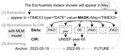
Figure 1: Overview of our 3-step pipeline for temporal tagging consisting of extraction of temporal expressions (step 1), normalization to a context-independent representation (CIR) using a slot-based masked language model (step 2) and anchoring given a reference time and further contextual cues (step 3).

We propose a new multilingual normalization method which can make use of labeled data from many languages by training a neural transformer model with a masked language modeling (MLM) objective. Thus, we adopt the MLM objective function for a new purpose: TE normalization.

To the best of our knowledge, this is the first work that uses neural networks for TE normalization. For this, as shown in Figure 1 and detailed below, we split the normalization task into two steps: normalization to a context-independent representation (CIR) and anchoring this representation using the document context.

The main contribution of this paper is our novel neural normalization method based on masked language modeling. For this, we create a large-scale multilingual dataset with weakly-supervised annotations of TEs and their normalized values in 87 languages. Our extensive set of experiments across 17 languages demonstrates that our multilingual method robustly works for many languages and outperforms the state of the art for multilingual temporal tagging, HeidelTime Strötgen and Gertz (2015), especially for low-resource languages by more than 33 $F_{1}$ on average. Further, we explore different training and decoding strategies for our model. The code for our models and the weakly- supervised data is publicly available.

2 Related Work

TE Normalization. Besides rule-based systems Chang and Manning (2012); Strötgen and Gertz (2013), one normalization method for TEs are context-free grammars Bethard (2013); Lee et al. (2014) which are independent of the extraction method. However, they are even more language-specific than rule-based systems and hardly generalizable to new languages. Laparra et al. (2018) used a rule-based procedure for English TE normalization based on the SCATE format proposed by Bethard and Parker (2016). While their method could be extended to multilingual applications, no annotated data for other languages is available in the SCATE format, and it is mostly incompatible with the predominant TimeML Pustejovsky et al. (2005) annotation format. Therefore, we will focus on the TimeML format in this work and present the first neural approach to TE normalization.

Masked Language Modeling (MLM). The MLM paradigm gains a lot of attention Sun et al. (2021) due to popular language models like BERT Devlin et al. (2019) This leads to active research on using MLM to solve further tasks like text classification Brown et al. (2020), named entity recognition Ma et al. (2021) and relation extraction Han et al. (2021), also in low-resource languages (Hedderich et al., 2021). In this work, we adopt it to TE normalization for the first time.

3 Background on Temporal Tagging

Temporal tagging addresses the detection, classification and normalization of temporal expressions in unstructured texts — often following the TimeML specifications Pustejovsky et al. (2005).

TimeML’s most important attributes are type (the class of an expression, e.g., Date, Time, Duration or Set), and value (the normalized meaning of an expression, e.g., YYYY-MM-DD for specific days, such as 2022-05-01 for May 1, 2022). While some TEs contain all necessary information for the normalization, e.g., “May 1, 2022”, many expressions are incomplete w.r.t. the temporal information required for a normalization. An example is a relative expression like “yesterday” which needs an anchor point. Given the anchor point May 1, 2022, for example from the document creation time, “yesterday” should be annotated with type=Date and value=2022-04-30.

Determining the anchor point can be challenging as it requires additional context information that could be given anywhere in the document. Therefore, systems for TE normalization, such as HeidelTime Strötgen and Gertz (2013), create an intermediate context-independent representation (CIR) of the value. In the syntax of HeidelTime, the expression yesterday would result in a CIR of UNDEF-last-day. Similarly, an underspecified expression, such as “May” would be represented with a CIR of UNDEF-year-05. Note that such a syntax for CIRs is language-independent. See Appendix A for more details. To determine the final value, the CIR needs to be anchored given, e.g., a reference date and further cues (such as tense information).

4 Approach

We propose to approach multilingual temporal tagging in three steps as shown in Figure 1: (1) Extraction of temporal expressions and their types using a multilingual sequence tagger; (2) Normalization of TEs to CIRs with our novel MLM-based normalization model; (3) Anchoring of CIRs given a reference time, e.g., using HeidelTime rules.

Our main contribution is a neural model for the second subtask, the normalization to a CIR. To the best of our knowledge, this has not been addressed with neural networks before. In this section, we detail all components of our approach. Information on the models that we apply for the first and third subtasks as well as an ablation study of directly predicting the normalized anchored value (without CIRs) are given in Section 5.

Masked Language Modeling.

We model the task of assigning CIRs to temporal expressions as masked language modeling. In particular, we add TimeML annotations as inline information to the text sequences and mask the value field for prediction, e.g., "… <TIMEX3 type="DATE" value="MASK">yesterday</TIMEX3> …". Note that those annotations could be the ground-truth annotations when applying the model on gold temporal expressions or predicted temporal expressions when using the model in the 3-step pipeline as described above. In our experiments, we train a transformer model for CIR prediction using the masked language modeling (MLM) objective.

Slot-Based Value Representation.

Using only a single mask token for the whole CIR would require the model to store all possible CIRs in its vocabulary. Since it is not possible to enumerate, i.a., all possible dates, we model the CIRs as a fixed-length sequence of slots. In particular, we define 11 slots and use regular expressions to split the value field into slots in the training data. Figure 1 shows an example for the CIR “UNDEF-year-05” that is represented as the slots “ [PAD], [year], [05], [PAD], …, [PAD]”. Details on the slots and regular expressions are given in Appendix A. To cover the full vocabulary of CIRs, we introduce 200 new tokens to the vocabulary of the language model.

Curriculum Learning.

Our slot-based representation with 11 slots per CIR results in 11 masks. To train the model on this task, we apply curriculum learning in the first half of the training. In particular, we start with masking only a single slot of the CIR and steadily increase the number of masks up to the maximum of 11. For the second half of the training, masking is applied to all slots. We follow Devlin et al. (2019) and mask different parts of the input with different probabilities. In particular, we mask the value slots with a probability of 70%, annotated tokens with 15%, types with 10% and other text parts with 5%.

Inference and Decoding.

For inference, we first add 11 masks (i.e., one per slot) to the input sentence. They serve as value placeholders that need to be predicted. Then, we use the masked language model to predict the most probable sequence of slots for the CIR. To decode the sequence, we apply sequential left-to-right decoding of all masks by iteratively decoding the left-most mask and replacing the mask with its predicted value until all masks are resolved. We compare this to two alternative decoding strategies: (i) decoding all masks simultaneously, (ii) training a conditional random field model that takes the logits as input and uses the Viterbi algorithm to determine the most probable sequence of predictions Lafferty et al. (2001).

5 Experiments

This section describes our experiments and discusses the results. We compare our model to HeidelTime Strötgen and Gertz (2013), the current state of the art for multilingual temporal tagging. For evaluation, we use the TempEval3 evaluation script UzZaman et al. (2013) and report strict, relaxed and type $F_{1}$ for the extraction and value $F_{1}$ for our normalization experiments, respectively.

Evaluation Data.

Our models are evaluated on gold-standard corpora in 17 languages. Details on the corpora are given in Appendix B.2. We divide the languages into high- and low-resource depending on whether manually created HeidelTime rules are available for the respective language.

Training Data.

For training the normalization model, we create a large-scale weakly-supervised dataset covering 87 languages. Reasons are that (i) existing gold training data is too small to cover the wide range of different values and (ii) CIRs are not part of existing annotations. For all languages, we take the data from GlobalVoices (news-style documents) and Wikipedia (narrative-style documents), use spacy for tokenization and HeidelTime for the annotation with temporal expressions. The number and quality of annotations is highly dependent on the amount of available data for that language and the quality of HeidelTime’s rules. Details on the weakly-supervised data are given in Appendix B.1.

	HeidelTime				Mono+Our				Multi+Our				Gold+Our
	Str.	Rel.	Type	Val.	Str.	Rel.	Type	Val.	Str.	Rel.	Type	Val.	Val.
de (N)	69.7	79.3	75.4	62.4	75.4	85.9	80.6	61.5	70.9	82.6	76.2	59.5	74.1
de (W)	88.5	94.3	89.0	84.8	89.6	97.0	96.0	83.8	88.9	96.7	95.4	85.7	87.5
en (N)	81.8	90.7	83.3	78.1	85.7	92.3	86.5	72.5	82.0	88.9	82.8	70.5	79.0
en (W)	90.6	94.3	90.6	94.3	93.1	96.6	93.1	89.7	94.7	98.3	87.7	94.2	94.2
es (N)	83.7	90.2	86.1	80.9	89.6	94.5	91.4	79.0	89.3	94.2	90.0	77.1	84.4
et (N)	42.4	57.4	51.3	44.0	3.3	28.0	24.4	9.6	55.5	78.0	72.0	45.2	64.8
fr (N)	85.6	90.6	82.3	73.3	82.5	88.1	79.7	67.9	82.4	89.8	76.9	61.4	68.0
hr (W)	93.3	95.8	94.6	85.7	84.1	90.8	89.5	74.6	86.3	91.7	90.1	75.7	84.7
it (N)	84.4	92.9	83.5	74.1	69.8	81.4	73.7	60.4	76.8	82.4	78.4	67.2	75.3
nl (N)	54.0	91.3	79.0	44.4	61.4	73.0	67.2	42.7	76.0	82.7	81.4	53.5	64.6
pt (N)	71.3	80.9	76.5	63.2	87.1	91.2	85.0	68.7	87.1	91.1	86.5	68.7	76.6
vi (W)	92.6	89.5	96.6	91.6	87.6	85.0	89.8	83.5	91.5	93.8	92.6	90.8	91.2
avg.	78.2	87.3	82.4	75.6	75.8	83.7	79.7	66.2	81.8	89.2	84.2	70.7	78.7
	HeidelTime-auto				Mono+Our				Multi+Our				Gold+Our
	Str.	Rel.	Type	Val.	Str.	Rel.	Type	Val.	Str.	Rel.	Type	Val.	Val.
ca (N)	28.1	62.8	61.1	43.6	29.5	64.3	62.3	40.2	77.3	87.8	82.5	59.7	67.9
el (W)	2.2	4.9	4.9	1.3	47.0	88.2	86.1	64.6	81.7	92.0	90.2	70.6	83.7
eu (N)	22.5	26.8	23.9	18.3	0.0	0.0	0.0	0.0	59.7	70.2	66.0	45.0	51.2
id (N)	19.7	54.7	44.5	40.1	17.4	39.7	30.6	25.6	49.7	79.5	63.9	46.9	64.8
pl (N)	18.8	27.2	16.5	11.2	86.1	92.5	87.6	58.7	86.7	92.2	87.7	59.0	66.0
ro (N)	3.2	19.5	16.7	5.5	3.8	22.6	37.0	7.7	9.8	47.2	39.1	19.7	54.6
ua (W)	1.6	2.8	2.2	1.2	80.2	90.6	87.5	63.6	79.4	90.7	88.8	65.4	74.5
avg.	12.7	28.4	24.3	17.3	37.7	56.8	55.9	37.2	63.5	79.9	74.0	50.9	66.1

Table 1: Detailed overview of our results for extraction (Str., Rel., Typ.) and normalization (Val.) per language for News and Wiki domains. The upper and lower parts display high- and low-resource languages, respectively.

3-Step Pipeline for Temporal Tagging.

Both our temporal expression extraction and normalization models are based on the mulitlingual XLM-R transformer Conneau et al. (2020).

We model the TE extraction as a sequence-labeling problem following Lange et al. (2020). For this, we convert the annotated corpora into the BIO format. For the monolingual setting (Mono), we train one model per language on the gold-standard resources if available or the weakly-supervised data otherwise. For the multilingual setting (Multi), we train a single model on the combined training resources of all languages.

For the normalization to CIRs, we train our proposed model with masked language modeling (see Section 4). In our experiments, we evaluate this model in combination with the multilingual extraction model (Multi+Our) as well as in combination with the gold boundaries for temporal expressions (Gold+Our) which serves as an upper bound.

For anchoring CIRs, we use rules similar to HeidelTime’s rules. In particular, anchor dates can be given by the document creation time or by previous temporal expressions Strötgen and Gertz (2016).

Results.

Table 1 gives an overview of our experimental results. Multilingual extraction outperforms monolingual extraction, probably because the model is able to use knowledge from different languages. Our multilingual model achieves +2 $F_{1}$ for high-resource and +51 $F_{1}$ for low-resource languages compared to HeidelTime.

The normalization results are given in the Val. columns of Table 1. Our masked language model is matching HeidelTime’s performance rather close for high-resource languages and outperforms it for low-resource languages with an increase of 33 $F_{1}$ points on average with our multilingual extraction model. Note that our models are multilingual, thus, we can use the same model for all languages. The upper bound of using gold extractions (Gold+Our) shows that the extraction part still offers room for future improvements.

Note that HeidelTime with automatically created rules has a poor performance for some low-resource languages (el, ro, ua). This is similar to the observations by Grabar and Hamon (2019) who found that “[e]xploitation of this automatically built system produced no results when applied to the Ukrainian data.” For those languages, the automatic rule generation is not good enough in practice which emphasizes the need for multilingual systems like our model.

Ablation Studies.

As our proposed model consists of multiple components, we now investigate their individual effects in more detail. The results for our ablation studies are given in Table 2.

First, we test different decoding strategies as described in Section 4. We find that sequential decoding works best. However, it also requires more computation time. A cheaper alternative with only minor performance decreases is the simultaneous decoding of all masks.

Second, we analyze the impact of different value representations by comparing our proposed approach with CIR and slot tokenization to (i) tokenization of values using the standard XLM-R tokenizer instead of pre-defined slots (w/o Our Slots), and (ii) training a model to directly predict the anchored value without CIRs in between (w/o Our CIR). For (i), we find that our slot method has major advantages when processing narrative texts, such as Wikipedia, due to the higher amount of relative expressions (cf., Table 3 in Appendix B.3), that are tokenized into many subtokens (up to 34, instead of 11 when using our slots). For (ii), we add the document creation time to the input so that the model has more temporal information to predict the fully normalized value directly instead of a CIR. However, we find that current transformers are not able to correctly incorporate this information in a combined normalizing+anchoring step and mostly predict a memorized, incorrect value. Thus, using CIRs as an intermediate step is important for neural temporal tagging.

Third, we investigate the training strategy and training data. Our curriculum learning has advantages for low-resource languages as it reduces the training complexity which helps for the difficult adaptation to languages with few resources. Weakly-supervised training data is required, as the amount of gold-standard data is too small to train the MLM model. Finetuning the trained MLM model further on gold data (Weak+Gold) decreases performance slightly. Training the model on monolingual data only also decreases performance, highlighting the prospects of our multilingual approach.

Finally, we compare our models to an encoder-decoder model, i.e., an autoregressive language model that we adapt to TE normalization. For this, we follow the entity linking approach from De Cao et al. (2021) and train a BART encoder-decoder model (Lewis et al., 2020) for constrained decoding against a subspace of normalized TEs with our weakly-supervised data. We add the document creation time to the input, mark the extracted annotations and keep other TEs in the context, as in our other experiments. Given the gigantic amount of possible temporal expressions, e.g., there are roughly 32M seconds in a single year, we have to prune the search space to a reasonable size. Thus, we do not use time expressions of hour and smaller granularities and restrict the search space to years and months from 1 AD to 2100. Finer elements like weeks, days and daytimes are added for years between 2000 and 2026. We use durations for all defined units with numbers up to 10,000, e.g., 10,000 days. With this, we prune the search space to 1.4B terms which we store in a prefix tree. This results in an acceptable inference speed with BEAM search (5 beams). It takes roughly twice as long as our sequential MLM decoding. Note that this BART model has more parameters (400M) than the base version of XLM-R (270M) that we use in our model. The results are shown in the lower part of Table 2. We see, that our proposed MLM normalization model outperforms the BART model by a large margin. Nonetheless, the encoder-decoder model performs comparable to our model variant that directly predicts fully-normalized expressions. This clearly highlights the need for normalizing to CIRs before anchoring temporal expressions.

	News		Wiki		Low-R.
	de	en	de	en	ca	eu
Our	74.1	79.0	87.5	94.2	67.9	51.2
Decoding Strategy (Our uses Sequential)
w/ Simultaneous	73.3	78.3	87.5	93.5	68.1	50.4
w/ Viterbi	73.3	78.3	87.5	94.2	67.9	50.4
Value Representation
w/o Our Slots	71.9	77.9	83.3	92.8	63.7	27.8
w/o Our CIR	68.5	68.0	66.5	55.7	41.6	21.2
Training Strategy
w/o Curriculum	72.1	80.4	85.5	94.4	64.7	29.3
Training Data (Our uses Weak)
Weak + Gold	68.3	76.1	58.2	93.3	-	-
only Gold	14.2	13.8	6.7	3.6	-	-
only Monolingual	63.1	76.8	86.8	91.4	29.2	8.9
Encoder-Decoder Model
Monolingual	59.3	67.4	49.4	59.6	2.2	7.3
Multilingual	63.5	63.0	49.0	58.5	54.8	25.2

Table 2: Ablation study for our model components (Value $F_{1}$) on gold extractions. Low-R. stands for low-resource languages without gold training data.

6 Conclusion

In this paper, we introduced a new method for normalizing temporal expressions based on masked language modeling and a new slot-based prediction scheme of context-independent representations. With this approach, we were able to train a single multilingual model for the task. We evaluated our method in 17 languages and set the new state of the art in low-resource languages with massive improvements of 35 $F_{1}$ points on average. The success of our method demonstrates the potential of neural networks for temporal normalization and we are convinced that it will enable future research on this topic. An interesting research direction is the joint modeling of extraction and normalization.

Limitations

Our experiments are focused on Indo-European languages due to the lack of publicly available, labeled data points in other languages. Exceptions for which we could test zero-shot transfer were Basque, Estonian, Indonesian and Vietnamese. Even though, our model is working for these languages, it is not clear if the multilingual models transfer to all languages seen in the pre-training or by our weak supervision. The training of the multilingual models requires a considerable number of computational resources (up to 1.5 GPU days), which might not be available for all people/organizations. By publishing our model, we hope to lower the barrier for this kind of research by providing a pre-trained starting point. An in-depth error analysis to better understand which types of temporal expressions are well or less well covered in which language by our model was not performed. We are full of hope that such analyses can be tackled by users of our models who have the required language skills so that the analysis does not have to be limited to English.

Appendix A Slot Tokenization of CIRs

In this section, we describe our slot-based tokenization of the context-independent representation (CIR) of values as introduced in Section 3 and Section 4 of the main paper.

A.1 Overview of Slots

We use the following 11 slots to represent CIRs values. These slots are then used for masking during training and inference with our normalization model (which basically is a masked language model).

SB:

This slot can contain BC information of years (e.g., as in BC4000 for the year 4000 BC) or the duration markers P and PT. Moreover, mathematical operations like PLUS are covered as used in relative expression involving offset computations (e.g., this-day-plus-2 for the day after tomorrow) and holiday names (EasterSunday).

SD1, SD2:

These slots are used to represent 4-digit year numbers (SD1 = 20 and SD2 = 22 for the year 2022) by splitting the 4-digit number into two 2-digit numbers. This helps to generalize to unseen years as fewer parameters have to be learned. In addition, we use SD1 to mark reference expressions like PAST_REF. For underspecifed expressions like UNDEF-this-day, this is stored in SD1 and day in SD2. Moreover, SD1 and SD2 are used to store numbers of DURATION expressions.

SD3, SD4:

Analogously to SD1 and SD2 that are used to store year information, SD3 is used for months and SD4 for days.

ST1, ST2, ST3:

Temporal information from expressions of type TIME that are smaller than day granularity are stored in the ST slots. For example, the hour information of 24:00 and the daytime information, such as EV is stored in ST1. Information on minutes and seconds is stored in ST2 and ST3, respectively. Moreover, these slots are used to cover additional units in durations, such as in P1D2H (1 day and 2 hours).

SA1, SA2, SA3:

Finally, some CIRs include function calls which can be augmented with arguments that we store in the SA slots. For example, the argument 2 of this-day-plus-2 is stored in SA1. Other function calls are used to compute days with respect to holidays like EaserSunday or specific weekdays.

Note that slots can be optional depending on the temporal expression. For example, the value 2022 representing the year 2022 would only require SD1 and SD2. All other slots are set to a padding value [PAD] then which allows a fixed-sized representations of CIRs that can be predicted with our masked language model.

Examples.

The following examples show temporal expressions, their corresponding CIRs and the tokenization into our slots. Note that there is no need to capture terms like UNDEF in our slots as the presence of words like this, next or last in a CIR implies the existence of UNDEF in the CIR. This information can be reconstructed when obtaining a CIR from our slots. This also includes -- to separate numbers as in YYYY-MM-DD values, REF in reference expressions and T for time information. We use the following format to give examples for our CIR conversion: Text $\rightarrow$ CIR $\rightarrow$ Slot Sequence

• Now …
  $\rightarrow$ PRESENT_REF
  $\rightarrow$ SD1=PRESENT

• … for 1000 days …
  $\rightarrow$ P1000D
  $\rightarrow$ SB=P, SD1=10, SD2=00, SD4=D

• … for one and a half day …
  $\rightarrow$ P1D12H
  $\rightarrow$ SB=P, SD1=1, SD4=D, ST1=12, ST2=H

• … in 1000 BC …
  $\rightarrow$ BC1000
  $\rightarrow$ SB=BC, SD1=10, SD2=00

• … on the morning of March 15, 2022 …
  $\rightarrow$ 2022-03-15TMO
  $\rightarrow$ SD1=20, SD2=22, SD3=03, SD4=15, ST1=MO

• On March 15, …
  $\rightarrow$ UNDEF-year-03-15
  $\rightarrow$ SD1=year, SD3=03, SD4=15

• … the day after tomorrow …
  $\rightarrow$ UNDEF-this-day-PLUS-2
  $\rightarrow$ SB=PLUS, SD1=this, SD2=day, SA1=2

• … at Pentecost …
  $\rightarrow$ UNDEF-year-00-00 funcDate… …Calc(EasterSunday(YEAR, 49))
  $\rightarrow$ SB=EasterSunday, SD1=year, SD2=00, SA1=49

A.2 Regular expressions

In the following, we will describe the six regular expressions used to split CIR values from HeidelTime outputs into our slots for the weakly-supervised training data.

Notation.

For readability, we define the following groups to capture temporal units and other fixed names. Note that these are used across languages. For example, the German expression Montag would still be represented with monday.

⬇

UNITS = (H|D|DE|DT|M|C|Y|

C|CE|W|WE|Qu|Q|S)

UNITS_F = (day|month|year|

decade|century|week|

weekend|quarter|

hour|minute|second)

DAYTIME = (NI|AF|MO|EV|MD|MI)

SPECIAL = (SP|SU|FA|AU|WI|

H1|H2|Q1|Q2|Q3|Q4|H|Q)

NAMES = (monday|tuesday|

wednesday|thursday|

friday|saturday|sunday|

january|february|march|

april|may|june|july|

august|september|

october|november|december)

In the following, $DX(n)$ marks the $n$-th group captured by the regular expression $DX$.

$D1$: References.

The first regular expression $D1$ is used to capture simple reference expressions that refer to uncertain points in time.

⬇

D1 = (PRESENT|PAST|FUTURE)_REF

Slots: SD1=D1(1)

$D2$: Explicit Dates.

The second regular expression $D2$ detects explicit values that do not need further normalization, such as days in the YYYY-DD-MM format, e.g., 20222-03-15.

⬇

D2 =(BC)?(\d\d?|XX)?(\d\d|XX)?

(?:-(W)?(\d\d?|XX|SPECIAL))?

(?:-(\d\d?|XX|WE))?\)?

(?:T(\d\d|X|DAYTIME|XX)?

(?::(\d\d))?

(?:(?::|-)(\d\d))?)?

Slots: SB=D2(1), SD1=D2(2),

SD2=D2(3), SD3=D2(5), SD4=D2(6),

ST1=D2(7), ST2=D2(8),

ST3=D2(9)|D2(4)

$P1$: Durations.

The third regular expression $P1$ detects expressions of type Duration, e.g., P1D2H. These are defined as P<number><unit> for units of at least day granularity and PT<number><unit> for smaller granularities. We capture up to two different units P1D2H (1 day and 2 hours) but ignore further units that are theoretically defined in the TimeML specifications but do not occur often in practice (in our datasets those did not occur at all).

⬇

P1 = (P|PT)(\d\d?|X|XX)

(\d\d|\.)?(\d\d?)?)?(UNITS)?

(\d\d?)?(UNITS)?

Slots: SB=P1(1), SD1=P1(2),

SD2=P1(3), SD3=P1(4), SD4=P1(6),

ST1=P1(5), ST2=P1(7)

$D3$: Relative Dates.

While the previous regular expressions $D1$, $D2$ and $P1$ follow the TimeML specifications and capture fully normalized expressions, i.e., anchored values, the following regular expressions capture CIRs as used internally by HeidelTime. They represent relative expressions that need to be anchored.

$D3$ detects relative expressions with respect to a certain point in time, such as this-day-plus-2 (the day after tomorrow).

⬇

D3 = UNDEF-(this|next|last|REF|

REFUNIT|REFDATE)?-?

(UNITS_F|SPECIAL)?-??

(NAMES|SPECIAL)|XX|\d\d?)?

(?:-?(\d\d?|XX))?

(?:-(PLUS|MINUS|LESS)-(\d\d?)-?

(\d\d?)?-?(\d\d?)?)?\)?

(?:T(\d\d?|X|DAYTIME|XX)?

(?::(\d\d?|XX))?(?:(?::|-)

(\d\d|XX))?)

Slots: SB=D3(5), SD1=D3(1),

SD2=D3(2), SD3=D3(3), SD4=D3(4),

ST1=D3(9),ST2=D3(10),ST3=D3(11),

SA1=D3(6), SA2=D3(7), SA3=D3(8)

$D4$: Relative Dates (coarse).

$D4$ captures underspecified expressions like May that is missing year information and would be represented with the CIR UNDEF-year-05.

⬇

D4 = UNDEF-(year|decade|century?)

-?(\d\d?|X)?-?(\d\d?|X)?-?

(\d\d?|X|SPECIAL)?\)?

(?:T(\d\d?|X|DAYTIME)?

(?::(\d\d?|XX))?

(?:(?::|-)(\d\d|XX))?)?

Slots: SD1=D4(1), SD2=D4(2),

SD3=D4(3), SD4=D4(4),

ST1=D4(5), ST2=D4(6), ST3=D4(7)

$D5$: Holidays and functions.

Finally, $D5$ covers special functions used by HeidelTime. These functions are used to compute days with respect to weekdays and moveable feasts like EasterSunday that refer to different days depending on the year. For example, the earliest possible date of Easter Sunday is March 22 and the latest is April 25 in the Gregorian calendar. The concrete date is then computed by an external function given a year.

⬇

D5 = (UNDEF-year|UNDEF-this-year|

UNDEF-century\d\d|\d\d\d\d)-

(\d\d)-00 funcDateCalc\((

WeekdayRelativeTo|

EasterSundayOrthodox|

EasterSunday|

ShroveTideOrthodox)

\(YEAR(?:(?:-(\d\d)))?

(?:-(\d\d))

(?:,\s?(-?\d\d?))?

(?:,\s?(-?\d\d?))?

(?:, (true|false))?\)\)

Slots: SB=D5(3), SD1=D4(1),

SD2=D4(2), SD3=D4(5),

SD4=D4(7), ST1=D4(3),

SA1=D5(6), SA2=D5(7), SA3=D5(8)

Appendix B Data Statistics

B.1 Weakly-Supervised Data

As detailed in Section 5, we create weakly-supervised data to train our normalization model, as the gold standard is too small and is not annotated with CIRs which are required by our method. For all languages, we take the data from GlobalVoices (news-style documents) and Wikipedia (narrative-style documents), use spacy for tokenization and our HeidelTime version that outputs CIRs for the annotation with temporal expressions. The sizes of our weakly-supervised data for each language are given in Table 4.

B.2 Gold-Standard Data

Detailed information on the datasets used in this paper (their languages, domains, sizes and references) are provided in Table 5. Note that all corpora come from the news domain except the WikiWars corpora that are based on Wikipedia articles.

B.3 Distribution of Explicit and Relative Values

The distribution of explicit and relative values has a large impact on the normalization performance of different models, as shown in our ablation study in Section 5. Exemplarily, we analyze their distribution in the German and English datasets for which we have data from two domains: News and Wikipedia. The results are given in Table 3. We see, that the Wikipedia corpora contain a much larger percentage of relative values as these articles often follow a narrative structure (cf., (Strötgen and Gertz, 2016).

	De	En
News	67.1 / 32.9	52.3 / 47.7
Wiki	47.6 / 52.4	44.2 / 55.8

Table 3: Distribution of explicit / relative values according to HeidelTime by domains (in %).

Appendix C A Note on Adopting HeidelTime

In our experiments, we used a modified version of HeidelTime. First, we implemented a new UIMA collection reader based on spacy as an alternative to the TreeTagger that has a restrictive license. This results in a slightly different sentence segmentation and tokenization, and, thus, minor differences in performance. For example, the original HeidelTime achieves 63.47 $F_{1}$ on the Portuguese test data, while our spacy version achieves 63.24 $F_{1}$ as one additional false positive expression was annotated due to different sentence boundaries. Second, we adapted HeidelTime to output its internal CIRs for the TimeML values, such that we can create our weakly-supervised training data.

The rather low performance of our models and HeidelTime for the high-resource languages Estonian (et) and Dutch (nl) can be explained by poor data quality. An inter-annotator agreement of 44 $F_{1}$ was reported for the Estonian corpus Orasmaa (2014), which is close to our results. The Dutch data was translated from English and automatically annotated via cross-lingual projections Minard et al. (2016), which may reduce the annotation quality. Note, that only the first five sentences for each document were annotated in the Meantime corpora (it and nl). We restricted our evaluation to these annotated parts accordingly.

Rank	Lang	#Ann.
1	de	870897
2	en	542087
3	fr	284871
4	ar	280446
5	es	250871
6	pt	215209
7	it	199236
8	nl	194944
9	ru	122884
10	zh	105421
11	hr	50233
12	ro	33545
13	vi	22048
14	af	21081
15	mk	19539
16	tr	19532
17	gl	17416
18	ca	16747
19	bn	16284
20	cy	14738
21	bg	14550
22	et	13948
23	sv	13705
24	id	13031
25	da	12919
26	fy	12852
27	pl	11283
28	fa	11041
29	eu	10992

Rank	Lang	#Ann.
30	ne	10750
31	ms	10017
32	mg	9271
33	kk	8080
34	hi	7762
35	eo	7353
36	ur	6228
37	hu	5871
38	sq	5760
39	sk	5172
40	sr	4276
41	ka	4247
42	el	4217
43	he	4057
44	sw	3979
45	ja	3696
46	br	3582
47	uz	3361
48	th	3162
49	cs	3096
50	ga	2799
51	mn	2778
52	gd	2772
53	lt	2734
54	mr	2623
55	la	1876
56	uk	1673
57	hy	1642
58	ta	1556

Rank	Lang	#Ann.
59	my	1103
60	ml	1079
61	kn	1029
62	fi	1017
63	oa	979
64	jv	968
65	ky	926
66	is	804
67	am	776
68	ku	557
69	so	506
70	yi	485
71	ko	483
72	si	442
73	ps	403
74	lo	354
75	km	350
76	su	335
77	lv	323
78	as	299
79	ug	283
80	sd	278
81	gu	258
82	ha	205
83	sl	125
84	yo	102
85	sa	24
86	or	19
87	xh	3

Table 4: Languages and the sizes of our weakly-supervised data.

Corpus	Language	#Annotations (train / test)	Reference
Corpora only used for evaluation
KRAUTS-DieZeit	German (de)	_ / 493	Strötgen et al. (2018)
TempEval-3 (platinum)	English (en)	_ / 137	UzZaman et al. (2013)
KOMPAS (test)	Indonesian (id)	_ / 192	Mirza (2016)
TimeBankCA	Catalan (ca)	_ / 1383	Saurı (2010)
EstTimeML	Estonian (et)	_ / 622	Orasmaa (2014)
EusTimeML	Basque (eu)	_ / 112	Altuna et al. (2020)
Fr TimeBank	French (fr)	_ / 423	Bittar et al. (2011)
Ro TimeBank	Romanian (ro)	_ / 151	Forăscu and Tufiş (2012)
PT-TimeBank (test)	Portuguese (pt)	_ / 151	Costa and Branco (2012)
WikiWars-EL (test)	Greek (el)	_ / 414	Kapernaros (2020)
Corpora split into train and test sets
Meantime (IT)	Italian (it)	229 / 244	Minard et al. (2016)
Meantime (NL)	Dutch (nl)	221 / 259	Minard et al. (2016)
TempEval-3 (ES)	Spanish (es)	730 / 551	UzZaman et al. (2013)
PolEval-2019	Polish (pl)	633 / 6011	Kocon et al. (2019)
WikiWars	English (en)	1378 / 1251	Mazur and Dale (2010)
WikiWars-DE	German (de)	1510 / 684	Strötgen and Gertz (2011)
WikiWars-HR	Croatian (hr)	724 / 677	Skukan et al. (2014)
WikiWars-UA	Ukrainian (ua)	454 / 2237	Grabar and Hamon (2019)
WikiWars-VI	Vietnamese (vi)	118 / 101	Strötgen et al. (2014)
Corpora only used for training
KRAUTS-Dolomiten	German (de)	388 / _	Strötgen et al. (2018)
Meantime (EN)	English (en)	472 / _	Minard et al. (2016)
TempEval-3 (train, en)	English (en)	1240 / _	UzZaman et al. (2013)
PT-TimeBank (train)	Portuguese (pt)	1127 / _	Costa and Branco (2012)
WikiWars-EL (train)	Greek (el)	1496 / _	Kapernaros (2020)

Table 5: Overview of datasets and details on their usage as training (extraction-only) or evaluation data.

References

- Altuna et al. (2020) Begoña Altuna, María Jesús Aranzabe, and Arantza Díaz de Ilarraza. 2020. Eustimeml: A mark-up language for temporal information in basque. Research in Corpus Linguistics, 8(1):86–104.
- Artetxe and Schwenk (2019) Mikel Artetxe and Holger Schwenk. 2019. Massively Multilingual Sentence Embeddings for Zero-Shot Cross-Lingual Transfer and Beyond. Transactions of the Association for Computational Linguistics, 7:597–610.
- Bethard (2013) Steven Bethard. 2013. A synchronous context free grammar for time normalization. In Proceedings of the 2013 Conference on Empirical Methods in Natural Language Processing, pages 821–826, Seattle, Washington, USA. Association for Computational Linguistics.
- Bethard and Parker (2016) Steven Bethard and Jonathan Parker. 2016. A semantically compositional annotation scheme for time normalization. In Proceedings of the Tenth International Conference on Language Resources and Evaluation (LREC’16), pages 3779–3786, Portorož, Slovenia. European Language Resources Association (ELRA).
- Bittar et al. (2011) André Bittar, Pascal Amsili, Pascal Denis, and Laurence Danlos. 2011. French TimeBank: An ISO-TimeML annotated reference corpus. In Proceedings of the 49th Annual Meeting of the Association for Computational Linguistics: Human Language Technologies, pages 130–134, Portland, Oregon, USA. Association for Computational Linguistics.
- Brown et al. (2020) Tom Brown, Benjamin Mann, Nick Ryder, Melanie Subbiah, Jared D Kaplan, Prafulla Dhariwal, Arvind Neelakantan, Pranav Shyam, Girish Sastry, Amanda Askell, Sandhini Agarwal, Ariel Herbert-Voss, Gretchen Krueger, Tom Henighan, Rewon Child, Aditya Ramesh, Daniel Ziegler, Jeffrey Wu, Clemens Winter, Chris Hesse, Mark Chen, Eric Sigler, Mateusz Litwin, Scott Gray, Benjamin Chess, Jack Clark, Christopher Berner, Sam McCandlish, Alec Radford, Ilya Sutskever, and Dario Amodei. 2020. Language models are few-shot learners. In Advances in Neural Information Processing Systems, volume 33, pages 1877–1901. Curran Associates, Inc.
- Chang and Manning (2012) Angel X. Chang and Christopher Manning. 2012. SUTime: A library for recognizing and normalizing time expressions. In Proceedings of the Eighth International Conference on Language Resources and Evaluation (LREC’12).
- Conneau et al. (2020) Alexis Conneau, Kartikay Khandelwal, Naman Goyal, Vishrav Chaudhary, Guillaume Wenzek, Francisco Guzmán, Edouard Grave, Myle Ott, Luke Zettlemoyer, and Veselin Stoyanov. 2020. Unsupervised cross-lingual representation learning at scale. In Proceedings of the 58th Annual Meeting of the Association for Computational Linguistics, pages 8440–8451, Online. Association for Computational Linguistics.
- Costa and Branco (2012) Francisco Costa and António Branco. 2012. TimeBankPT: A TimeML annotated corpus of Portuguese. In Proceedings of the Eighth International Conference on Language Resources and Evaluation (LREC’12), pages 3727–3734, Istanbul, Turkey. European Language Resources Association (ELRA).
- De Cao et al. (2021) Nicola De Cao, Gautier Izacard, Sebastian Riedel, and Fabio Petroni. 2021. Autoregressive entity retrieval. In 9th International Conference on Learning Representations, ICLR 2021, Virtual Event, Austria, May 3-7, 2021. OpenReview.net.
- Devlin et al. (2019) Jacob Devlin, Ming-Wei Chang, Kenton Lee, and Kristina Toutanova. 2019. BERT: Pre-training of deep bidirectional transformers for language understanding. In Proceedings of the 2019 Conference of the North American Chapter of the Association for Computational Linguistics: Human Language Technologies, Volume 1 (Long and Short Papers), pages 4171–4186, Minneapolis, Minnesota. Association for Computational Linguistics.
- Forăscu and Tufiş (2012) Corina Forăscu and Dan Tufiş. 2012. Romanian TimeBank: An annotated parallel corpus for temporal information. In Proceedings of the Eighth International Conference on Language Resources and Evaluation (LREC’12), pages 3762–3766, Istanbul, Turkey. European Language Resources Association (ELRA).
- Grabar and Hamon (2019) Natalia Grabar and Thierry Hamon. 2019. Wikiwars-ua: Ukrainian corpus annotated with temporal expressions. Computational Linguistics and Intelligent Systems, 2:22–31.
- Han et al. (2021) Xu Han, Weilin Zhao, Ning Ding, Zhiyuan Liu, and Maosong Sun. 2021. Ptr: Prompt tuning with rules for text classification. arXiv preprint arXiv:2105.11259.
- Hedderich et al. (2021) Michael A. Hedderich, Lukas Lange, Heike Adel, Jannik Strötgen, and Dietrich Klakow. 2021. A survey on recent approaches for natural language processing in low-resource scenarios. In Proceedings of the 2021 Conference of the North American Chapter of the Association for Computational Linguistics: Human Language Technologies, pages 2545–2568, Online. Association for Computational Linguistics.
- Kapernaros (2020) Emmanouil I. Kapernaros. 2020. Extending the temporal tagger heideltime for the greek language.
- Kocon et al. (2019) Jan Kocon, Marcin Oleksy, Tomasz Bernas, and Michał Marcinczuk. 2019. Results of the poleval 2019 shared task 1: Recognition and normalization of temporal expressions. Proceedings ofthePolEval2019Workshop, page 9.
- Lafferty et al. (2001) John D. Lafferty, Andrew McCallum, and Fernando C. N. Pereira. 2001. Conditional random fields: Probabilistic models for segmenting and labeling sequence data. In Proceedings of the Eighteenth International Conference on Machine Learning, ICML ’01, pages 282–289, San Francisco, CA, USA. Morgan Kaufmann Publishers Inc.
- Lange et al. (2020) Lukas Lange, Anastasiia Iurshina, Heike Adel, and Jannik Strötgen. 2020. Adversarial alignment of multilingual models for extracting temporal expressions from text. In Proceedings of the 5th Workshop on Representation Learning for NLP, pages 103–109, Online. Association for Computational Linguistics.
- Laparra et al. (2018) Egoitz Laparra, Dongfang Xu, and Steven Bethard. 2018. From characters to time intervals: New paradigms for evaluation and neural parsing of time normalizations. Transactions of the Association for Computational Linguistics, 6.
- Lee et al. (2014) Kenton Lee, Yoav Artzi, Jesse Dodge, and Luke Zettlemoyer. 2014. Context-dependent semantic parsing for time expressions. In Proceedings of the 52nd Annual Meeting of the Association for Computational Linguistics (Volume 1: Long Papers).
- Lewis et al. (2020) Mike Lewis, Yinhan Liu, Naman Goyal, Marjan Ghazvininejad, Abdelrahman Mohamed, Omer Levy, Veselin Stoyanov, and Luke Zettlemoyer. 2020. BART: Denoising sequence-to-sequence pre-training for natural language generation, translation, and comprehension. In Proceedings of the 58th Annual Meeting of the Association for Computational Linguistics, pages 7871–7880, Online. Association for Computational Linguistics.
- Ma et al. (2021) Ruotian Ma, Xin Zhou, Tao Gui, Yiding Tan, Qi Zhang, and Xuanjing Huang. 2021. Template-free prompt tuning for few-shot ner. arXiv preprint arXiv:2109.13532.
- Mazur and Dale (2010) Pawel Mazur and Robert Dale. 2010. WikiWars: A new corpus for research on temporal expressions. In Proceedings of the 2010 Conference on Empirical Methods in Natural Language Processing, pages 913–922, Cambridge, MA. Association for Computational Linguistics.
- Minard et al. (2016) Anne-Lyse Minard, Manuela Speranza, Ruben Urizar, Begoña Altuna, Marieke van Erp, Anneleen Schoen, and Chantal van Son. 2016. MEANTIME, the NewsReader multilingual event and time corpus. In Proceedings of the Tenth International Conference on Language Resources and Evaluation (LREC’16), pages 4417–4422, Portorož, Slovenia. European Language Resources Association (ELRA).
- Mirza (2016) Paramita Mirza. 2016. Recognizing and normalizing temporal expressions in indonesian texts. In Computational Linguistics, pages 135–147, Singapore. Springer Singapore.
- Orasmaa (2014) Siim Orasmaa. 2014. Towards an integration of syntactic and temporal annotations in Estonian. In Proceedings of the Ninth International Conference on Language Resources and Evaluation (LREC’14), pages 1259–1266, Reykjavik, Iceland. European Language Resources Association (ELRA).
- Pustejovsky et al. (2005) James Pustejovsky, Robert Ingria, Roser Saurí, José Castaño, Jessica Littman, Rob Gaizauskas, Andrea Setzer, Graham Katz, and Inderjeet Mani. 2005. The specification language TimeML. In The language of time: a reader, pages 545–557. Oxford University Press.
- Rahimi et al. (2019) Afshin Rahimi, Yuan Li, and Trevor Cohn. 2019. Massively multilingual transfer for NER. In Proceedings of the 57th Annual Meeting of the Association for Computational Linguistics, pages 151–164, Florence, Italy. Association for Computational Linguistics.
- Saurı (2010) Roser Saurı. 2010. Annotating temporal relations in catalan and spanish timeml annotation guidelines. Technical report, Technical report, Technical Report BM 2010-04, Barcelona Media.
- Skukan et al. (2014) Luka Skukan, Goran Glavaš, and Jan Šnajder. 2014. Heideltime. hr: extracting and normalizing temporal expressions in croatian. In Proceedings of the 9th Slovenian Language Technologies Conferences (IS-LT 2014), pages 99–103.
- Strötgen et al. (2014) Jannik Strötgen, Ayser Armiti, Tran Van Canh, Julian Zell, and Michael Gertz. 2014. Time for more languages: Temporal tagging of arabic, italian, spanish, and vietnamese. ACM Transactions on Asian Language Information Processing, 13(1).
- Strötgen and Gertz (2011) Jannik Strötgen and Michael Gertz. 2011. Wikiwarsde: A german corpus of narratives annotated with temporal expressions. In Proceedings of the conference of the German society for computational linguistics and language technology (GSCL 2011), pages 129–134. Citeseer.
- Strötgen and Gertz (2013) Jannik Strötgen and Michael Gertz. 2013. Multilingual and cross-domain temporal tagging. Language Resources and Evaluation, 47(2).
- Strötgen and Gertz (2015) Jannik Strötgen and Michael Gertz. 2015. A baseline temporal tagger for all languages. In Proceedings of the 2015 Conference on Empirical Methods in Natural Language Processing.
- Strötgen and Gertz (2016) Jannik Strötgen and Michael Gertz. 2016. Domain-sensitive temporal tagging, volume 9. Morgan & Claypool Publishers.
- Strötgen et al. (2018) Jannik Strötgen, Anne-Lyse Minard, Lukas Lange, Manuela Speranza, and Bernardo Magnini. 2018. KRAUTS: A German temporally annotated news corpus. In Proceedings of the Eleventh International Conference on Language Resources and Evaluation (LREC 2018), Miyazaki, Japan. European Language Resources Association (ELRA).
- Sun et al. (2021) Tianxiang Sun, Xiangyang Liu, Xipeng Qiu, and Xuanjing Huang. 2021. Paradigm shift in natural language processing. arXiv preprint arXiv:2109.12575.
- UzZaman et al. (2013) Naushad UzZaman, Hector Llorens, Leon Derczynski, James Allen, Marc Verhagen, and James Pustejovsky. 2013. SemEval-2013 task 1: TempEval-3: Evaluating time expressions, events, and temporal relations. In Second Joint Conference on Lexical and Computational Semantics (*SEM), Volume 2: Proceedings of the Seventh International Workshop on Semantic Evaluation (SemEval 2013), pages 1–9, Atlanta, Georgia, USA. Association for Computational Linguistics.