On slim rectangular lattices

Abstract.

Let $L$ be a slim, planar, semimodular lattice (slim means that it does not contain an ${\mathsf{M}}_{3}$-sublattice). We call the interval $I=[o,i]$ of $L$ rectangular, if there are complementary $a,b\in I$ such that $a$ is to the left of $b$.

We claim that a rectangular interval of a slim rectangular lattice is also a slim rectangular lattice. We will present some applications, including a recent result of G. Czédli.

In a paper with E. Knapp about a dozen years ago, we introduced natural diagrams for slim rectangular lattices. Five years later, G. Czédli introduced ${\mathcal{C}}_{1}$-diagrams. We prove that they are the same.

1. Introduction

In 2006, we started studying planar semimodular lattices in my papers with E. Knapp [10]–[14]. More than four dozen publications have been devoted to this topic since; see G. Czédli’s list
http://www.math.u-szeged.hu/~czedli/m/listak/publ-psml.pdf

An SPS lattice $L$ is a planar semimodular lattice that is also slim (it does not contain an $\mathsf{M}_{3}$-sublattice).

Following my paper with E. Knapp [13], a planar semimodular lattice $L$ is rectangular, if its left boundary chain has exactly one doubly-irreducible element other than the bounds (the left corner) and its right boundary chain has exactly one doubly-irreducible element other than the bounds (the right corner) and the two corners are complementary. An SR lattice $L$ is a rectangular lattice that is also slim.

Rectangular lattices are easier to work with than planar semimodular lattices, because they have much more structure. Moreover, a planar semimodular lattice has a (congruence-preserving) extension to a rectangular lattice, so we can prove many result for SPS lattices by verifying them for SR lattices (G. Grätzer and E. Knapp [13]).

It turns out that there is another way to obtain SR lattices from SPS lattices. Before we state it, we need a definition. Let $L$ be a planar lattice. We call the interval $I=[o,i]$ of $L$ rectangular, if there are complementary $a,b\in I$ such that the element $a$ is to the left of the element $b$.

Now we state a new property of SR lattices.

Theorem 1.

Let $L$ be an slim, planar, semimodular lattice and let $I$ be a rectangular interval of $L$. Then the lattice $I$ is slim and rectangular.

In a paper with E. Knapp about a dozen years ago, we introduced natural diagrams for SR lattices. Five years later, G. Czédli introduced ${\mathcal{C}}_{1}$-diagrams. We prove that they are the same.

We will present some applications, including a recent result of G. Czédli [4].

For the background of this topic and its applications outside lattice theory, see Section 1.2 of G. Czédli and G. Grätzer [5].

Statements and declarations

Data availability statement. Data sharing is not applicable to this article as no datasets were generated or analysed during the current study.

Competing interests. Not applicable as there are no interests to report.

Basic concepts and notation.

The basic concepts and notation not defined in this note are freely available in Part I of the book [7], see
arXiv:2104.06539
We will reference it as CFL2.

2. Fork extensions

We discuss in Section 4.3 of CFL2 a result of G. Czédli and E. T. Schmidt [6]: for an SPS lattice $L$ and covering square $C$ in $L$, we can insert a fork in $L$ at $C$ to obtain the lattice extension $L[C]$, which is also an SPS lattice, see Figure 1. In this figure, the elements of the covering square $C$ are grey filled, the elements of the fork are black filled. The third and fourth diagrams represent the same lattice, De gustibus non est disputandum.

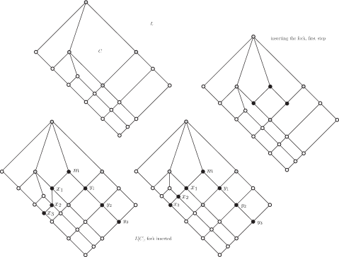
Figure 1. Inserting a fork into $L$ at $C$

As illustrated by Figure 2, we can sometimes delete a fork. Let $L$ be an SPS lattice and let $S$ be a covering $\mathsf{S}_{7}$ in $L$, with middle element $m$, left corner $a$ and right corner $b$. Let us assume that the top element $t$ of $S$ is minimal, that is, there is no $S^{\prime}$ a covering $\mathsf{S}_{7}$ with top element $t^{\prime}$ that is smaller: that is, $t^{\prime}<t$.

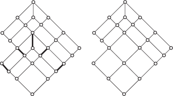
Figure 2. Deleting a fork

Lemma 2 (G. Czédli and E. T. Schmidt [6]).

Let $L$ be an SR lattice and let

$$S=\{o,m\wedge a,m\wedge b,a,b,m,t\}$$

be a minimal covering $\mathsf{S}_{7}$ in $L$. Then $L$ has a sublattice $L^{-}$ with a covering square

$$C=S-\{m,m\wedge a,m\wedge b\}=\{o,a,b,t\}$$

such that $L=L^{-}[C]$. In other words, we can delete the fork in $S$ and the lattice $L^{-}$ is the lattice $L$ with the fork deleted.

The structure of SR lattices is described as follows, see G. Czédli and E. T. Schmidt [6].

Theorem 3 (Structure Theorem).

A slim rectangular lattice $K$ can be obtained from a grid $G$ by inserting forks ($n$-times).

We thus associate a natural number $n$ with an SR lattice $K$; we call it the rank of $K$, and denote it by Rank(K). It is easy to see that the Rank(K) is well defined.

There is a stronger version of Theorem 3, implicit in G. Czédli and E. T. Schmidt [6]. We present it with a short proof.

Theorem 4 (Structure Theorem, Strong Version).

For every slim rectangular lattice $K$, there is a grid $G$, a natural number $n=\textup{Rank(K)}$, and sequences

(1) $$G=K_{1},K_{2},\dots,K_{n-1},K_{n}=K$$

of slim rectangular lattices and

(2) $$C_{1}=\{o_{1},c_{1},d_{1},i_{1}\},C_{2}=\{o_{2},c_{2},d_{2},i_{2}\},\dots,C_{n-1}=\{o_{n-1},c_{n-1},d_{n-1},i_{n-1}\}$$

of $4$-cells in the appropriate lattices such that

(3) $$G=K_{1},K_{1}[C_{1}]=K_{2},\dots,K_{n-1}[C_{n-1}]=K_{n}=K$$

and the principal ideals $\,\downarrow\!c_{n-1}$ and $\,\downarrow\!d_{n-1}$ are distributive.

Proof.

We prove by induction on $n$. If $n=0$, then $K$ is distributive by G. Grätzer and E. Knapp [13], so the statement is trivial. Now let us assume that the statement holds for $n-1$. Let $K$ be an SR lattice with $n$ covering $\mathsf{S}_{7}$-s. As in Lemma 2, we take $S$, a minimal covering $\mathsf{S}_{7}$ in $K$. Then we form the sublattice $K^{-}$ by deleting the fork at $S$. So we get a covering square $C=C_{n-1}=\{o_{n-1},c_{n-1},d_{n-1},i_{n-1}\}$ of $K^{-}$ such that $K=K^{-}[C]$. Since $K^{-}$ has $n-1$ covering $\mathsf{S}_{7}$-s, we get the sequence

$$G=K_{1},K_{1}[C_{1}]=K_{2},\dots,K_{n-2}[C_{n-2}]=K_{n-1}=K^{-},$$

which, along with $K=K^{-}[C]$, prove the statement for $K$. The minimality of $S$ implies that the principal ideals $\,\downarrow\!c_{n-1}$ and $\,\downarrow\!d_{n-1}$ are distributive. ∎

3. Proving Theorem 1

Theorem 1 obviously holds for grids.

Otherwise, we can assume that the SR lattice $K$ is not a grid, so $n=\textup{Rank(K)}>1$. Let $K^{-}$ be the lattice we obtain by deleting a minimal fork in $K^{-}$ at the covering square

$$C_{n-1}=\{o_{n-1},c_{n-1},d_{n-1},i_{n-1}\}.$$

We obtain $K$ from $K^{-}$ by inserting a fork at $C_{n-1}$. We add the element $m$ in the middle of $C_{n-1}$, and add the sequences of elements $x_{1},\dots$ on the left going down and $y_{1},\dots$ on the right going down as in Figure 1.

Let $I$ be a rectangular interval in $K$ with corners $a,b$, where $a$ is to the left of $b$. We want to prove that $I$ is an SR lattice. Of course, the lattice $I$ is slim.

We induct on $n=\textup{Rank(K)}$. There are three subcases.

Case 1. $I$ is disjoint to $\,\downarrow\!m$, as illustrated in Figure 3. Then the interval $I$ is not changed as we add the fork to $K^{-}$. By induction, $I$ is rectangular in $K^{-}$, therefore, $I$ is also rectangular in $K$.

Case 2. In Figure 4 (and Figure 5), the bold lines form the boundary of the rectangular sublattice $I$ in $K^{-}$, the elements of $C_{n-1}$ are grey filled, and the elements $m$, $x_{1}$, …, $y_{1}$, … are black filled. The element $m$ is internal in $I$, so the element $a$ is $c_{n-1}$ or it is to the left of $c_{n-1}$ and symmetrically, see Figure 4. Therefore, $C_{n-1}=[o_{n-1},i_{n-1}]_{K^{-}}$ is a covering square in ${K^{-}}$ and we obtain the interval $[o_{n-1},i_{n-1}]_{K}$ of $K$ by adding a fork to $C_{n-1}$ at $[o_{n-1},i_{n-1}]_{K^{-}}$. A fork extension of an SR lattice is also an SR lattice, so we conclude that $I$ is an SR lattice.

Case 3. $m$ is not an internal element of $I$ but some $x_{i}$ or $y_{i}$ is, see Figure 5, where $y_{2}$ is an internal element of $I$. By utilizing that $\,\downarrow\!d_{n-1}$ is distributive, we conclude that we obtain $I$ from $[o,i]_{K^{-}}$ by replacing a cover preserving $\mathsf{C}_{m}\times\mathsf{C}_{2}$ by $\mathsf{C}_{m}\times\mathsf{C}_{3}$, and so $I$ remains rectangular.

4. Applications of Theorem 1

The next statement follows directly from Theorem 1.

Corollary 5.

Let $L$ be an SPS lattice and let $I$ be a rectangular interval of $L$. Let (P) be any property of SR lattices. Then the property (P) holds for the lattice $I$.

Figure 3. Proving Theorem 1: Case 1

Figure 4. Proving Theorem 1: Case 2

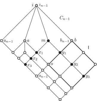
Figure 5. Proving Theorem 1: Case 3

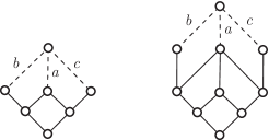
Figure 6. The lattice $\mathsf{S}_{7}$, two diagrams

For instance, let (P) be the property: the intervals $[o,a]$ and $[o,b]$ are chains and all elements of the lower boundary of $I$ are meet-reducible, except for $a,b$. Then we get the main result of G. Czédli [4].

Corollary 6.

Let $L$ be an SPS lattice and let $I$ be a rectangular interval of $L$ with corners $a,b$. Then $[o,a]$ and $[o,b]$ are chains and all the elements of the lower boundary of $I$ except for $a,b$ are meet-reducible.

Another nice application is the following.

Corollary 7.

Let $L$ be an SPS lattice and let $I$ be a rectangular interval of $L$ with corners $a,b$. Then for any $x\in I$, the following equation holds:

$$x=(x\wedge a)\vee(x\wedge b).$$

Here is a more elegant way to formulate the last result.

Corollary 8.

Let $L$ be an SPS lattice and let $a,b,c$ be pairwise incomparable elements of $L$. If $a$ is to the left of $b$, and $b$ is to the left of $c$, then

$$b=(b\wedge a)\vee(b\wedge c).$$

5. Special diagrams

5.1. Natural diagrams

SR lattices have some particularly nice diagrams such as the natural diagrams of my paper with E. Knapp [14], which laid the foundation of rectangular lattices. Natural diagrams were discovered more than a dozen years ago, many years before the appearance of it competitor, the $\mathcal{C}_{1}$-diagrams of G. Czédli—see the next section.

For an SR lattice $L$, let $\textup{C}_{\textup{l}}(L)$ be the lower left and $\textup{C}_{\textup{r}}(L)$ the lower right boundary chain of $L$, respectively, and let lc(L) be the left and rc(L) the right corner of $L$, respectively.

We regard $G=\textup{C}_{\textup{l}}(L)\times\textup{C}_{\textup{r}}(L)$ as a planar lattice, with $\textup{C}_{\textup{l}}(L)=\textup{C}_{\textup{l}}(G)$ and $\textup{C}_{\textup{r}}(L)=\textup{C}_{\textup{r}}(G)$. Then the map

(4) $$\psi\colon x\mapsto(x\wedge\textup{lc(L)},x\wedge\textup{rc(L)})$$

is a meet-embedding of $L$ into $G$; the map $\psi$ also preserves the bounds. Therefore, the image of $L$ under $\psi$ in $G$ is a diagram of $L$, we call it the natural diagram representing $L$. For instance, the second diagram of Figure 6 shows the natural diagram representing  $\mathsf{S}_{7}$.

Let $L$ be an SR lattice. By the Structure Theorem, Strong Version, we can represent $L$ in the form $L=K[C]$, where $K$ is an SR lattice, $C=\{o,c,d,i\}$ is a $4$-cell of $K$ satisfying that $\,\downarrow\!c$ and $\,\downarrow\!d$ are distributive. Let $\mathcal{D}$ be a diagram of $K$. We form the diagram $\mathcal{D}[C]$ by adding the elements $m,x_{1},\dots$, and $m,y_{1},\dots$, as in the last diagram of Figure 1, so that the lines spanned by the elements $m,x_{1},\dots$ and m, $y_{1},\dots$ are both normal.

Lemma 9.

Let $L$, $C$, $K$, $\mathcal{D}$, and $\mathcal{D}[C]$ be as in the previous paragraph. Then $\mathcal{D}[C]$ is a diagram of $L$.

Proof.

This is obvious. ∎

Lemma 10.

Let us make the assumptions of Lemma 13. If $\mathcal{D}$ is a natural diagram of $K$, then $\mathcal{D}[C]$ is a natural diagram of $L$.

Proof.

So let $\mathcal{D}$ be a natural diagram of $K$. Let the line $m,x_{1},\dots$ terminate with $x_{k_{l}}$ and the line $m,y_{1},\dots$ with $y_{k_{r}}$. We have to show that all the new elements in $L$ can be represented as a join $u_{l}\vee u_{r}$, where $u_{l}\in\textup{C}_{\textup{l}}(L)$ and $u_{r}\in\textup{C}_{\textup{r}}(L)$. Indeed, $m=x_{k_{l}}\vee x_{k_{r}}$. The others follow from the distributivity assumptions. ∎

$\mathcal{C}_{1}$-diagrams

This research tool, introduced by G. Czédli, has been playing an important role in some recent papers, see G. Czédli [2]–[4], G. Czédli and G. Grätzer [5], and G. Grätzer [8]; for the definition, see G. Czédli [2] and G. Grätzer [8].

In the diagram of an SR lattice $K$, a normal edge (line) has a slope of $45\degree$ or $135\degree$. Any edge (line) of slope strictly between $45\degree$ and $135\degree$ is steep.

Figure 6 depicts the lattice $\mathsf{S}_{7}$. A peak sublattice $\mathsf{S}_{7}$ (peak sublattice, for short) of a lattice $L$ is a sublattice isomorphic to $\mathsf{S}_{7}$ such that the three edges at the top are covers in the lattice $L$.

Definition 11.

A diagram of a slim rectangular $L$ is a ${\mathcal{C}}_{1}$-diagram, if the middle edge of a peak sublattice is steep and all other edges are normal.

In other words, an edge is steep if it is the middle edge of a peak sublattice; if an edge is not the middle edge of a peak sublattice, then it is normal.

Theorem 12.

Every slim rectangular lattice $L$ has a ${\mathcal{C}}_{1}$-diagram.

This was proved in G. Czédli [2]. My note [9] presents a short and direct proof.

6. Natural diagrams and ${\mathcal{C}}_{1}$-diagrams are the same

We start with a trivial statement.

Lemma 13.

Let us make the assumptions of Lemma 13. If $\mathcal{D}$ is a ${\mathcal{C}}_{1}$-diagram of $K$, then $\mathcal{D}[C]$ is a ${\mathcal{C}}_{1}$-diagram of $L$.

Now we state our second result on SR lattices.

Theorem 14.

Let $L$ be a SR lattice. Then a natural diagram of $L$ is a ${\mathcal{C}}_{1}$-diagram. Conversely, every ${\mathcal{C}}_{1}$-diagram is natural.

Proof.

Let us assume that the SR lattice $L$ can be obtained from a grid $G$ by adding forks $n$-times, where $n=\textup{Rank(L)}$. We induct on $n$. The case $n=0$ is trivial because then $L$ is a grid. So let us assume that the theorem holds for $n-1$.

By the Structure Theorem, Strong Version, there is a SR lattice $K$ and a $4$-cell $C=\{o,a,b,i\}$ of $K$ satisfying that $\,\downarrow\!c$ and $\,\downarrow\!d$ are distributive such that $K$ can be obtained from the grid $G$ by adding forks $(n-1)$-times and also $L=K[C]$ holds.

Now form the natural diagram $\mathcal{D}$ of $K$. By induction, it is a ${\mathcal{C}}_{1}$-diagram. By Lemma 9, the diagram $\mathcal{D}[C]$ is both natural and ${\mathcal{C}}_{1}$.

We prove the converse the same way. ∎

Natural diagrams exist by definition. So Theorem 12 also follows from Theorem 14.

G. Czédli [2] also defined ${\mathcal{C}}_{2}$-diagrams. A ${\mathcal{C}}_{1}$-diagram is ${\mathcal{C}}_{2}$, if any two edges on the lower boundary are of the same length.

We use Theorem 14 to prove two results of G. Czédli [2].

Theorem 15.

Let $L$ be a SR lattice. Then $L$ has a ${\mathcal{C}}_{2}$-diagram.

Proof.

Let $C_{l}$ and $C_{r}$ be chains of the same length as $\textup{C}_{\textup{l}}(L)$ and $\textup{C}_{\textup{r}}(L)$, respectively. Then $\textup{C}_{\textup{l}}(L)\times\textup{C}_{\textup{r}}(L)$ and $C_{l}\times C_{r}$ are isomorphic, so we can regard the map $\psi$, see (4), as a map from $L$ into $C_{l}\times C_{r}$, a bounded and meet-preserving map. So the natural diagram it defines is the diagram of the lattice $L$.

If we choose $C_{l}$ and $C_{r}$ so that the edges are of the same size, we obtain a ${\mathcal{C}}_{2}$-diagram of the SR lattice $L$. ∎

Natural diagrams have a left-right symmetry. The symmetric diagram is obtained with the map

(5) $$\widetilde{\psi}\colon x\mapsto(x\wedge\textup{rc(L)},x\wedge\textup{lc(L)})$$

replacing (4).

Theorem 16 (Uniqueness Theorem).

Let $L$ be a slim rectangular lattice. Then the ${\mathcal{C}}_{2}$-diagram of $L$ is unique up to left-right symmetry.

References

- [1] G. Czédli, Finite convex geometries of circles. Discrete Mathematics 330 (2014), 61–75.
- [2] G. Czédli, Diagrams and rectangular extensions of planar semimodular lattices. Algebra Universalis 77 (2017), 443–498.
- [3] G. Czédli, Lamps in slim rectangular planar semimodular lattices. Acta Sci. Math. (Szeged) 87 (2021), 381-413.
-
[4]