Eigenvalue bounds of the Kirchhoff Laplacian

Abstract.

We prove the inequality $\lambda_{k}\leq d_{k}+d_{k-1}$ for all the eigenvalues $\lambda_{1}\leq\lambda_{2}\leq\cdots\leq\lambda_{n}$ of the Kirchhoff matrix $K$ of a finite simple graph or quiver with vertex degrees $d_{1}\leq d_{2}\leq\cdots\leq d_{n}$ and assuming $d_{0}=0$. A consequence in the graph case is that the pseudo determinant ${\rm Det}(K)$ counting the number of rooted spanning trees has an upper bound $2^{n}\prod_{k=1}^{n}d_{k}$ and that ${\rm det}(1+K)$ counting the number of rooted spanning forests has an upper bound $\prod_{k=1}^{n}(1+2d_{k})$.

1. The theorem

1.1.

Let $G=(V,E)$ be a quiver with $n$ vertices. Without self-loops, this is a finite multi-graph. Without self-loops and no multiple-connections, this is a finite simple graph. Denote by $\lambda_{1}\leq\lambda_{2}\leq\cdots\leq\lambda_{n}$ the ordered list of eigenvalues of the Kirchhoff matrix $K=B-A$, where $B$ is the diagonal vertex degree matrix with ordered vertex degrees $d_{1}\leq d_{2}\leq\cdots\leq d_{n}$ and where $A$ is the adjacency matrix of $G$.

1.2.

We assume $d_{0}=0$ so that $d_{1}+d_{0}=d_{1}$ and prove:

Theorem 1.

$\lambda_{k}\leq d_{k}+d_{k-1}$, for all $1\leq k\leq n$ and all quivers.

1.3.

For finite simple graphs, $k=n$ is the spectral radius estimate of Anderson and Morley [1]. It generalizes to quivers:

Lemma 1.

$\lambda_{n}\leq d_{n}+d_{n-1}$ for all quivers with $n$ vertices.

1.4.

The reason is that we can still factor $K=F^{T}F$ and that the spectral radius of $K=F^{T}F$ agrees with the spectral radius of $K_{1}=FF^{T}$ if $F$ is an incidence gradient matrix of the quiver and because the spectral radius of $K_{1}$ is bound above by the maximal absolute column sum in $K_{1}$, which is $d_{n}+d_{n-1}$.

1.5.

The case $k=1$ obviously holds because $\lambda_{1}=0$, and $k=2$ is a case for the Schur-Horn inequality [6] as $\lambda_{2}=\lambda_{1}+\lambda_{2}\leq d_{1}+d_{2}$. Already $\lambda_{3}\leq d_{3}+d_{2}$ goes beyond Schur-Horn. Any estimate $\lambda_{n}$ in terms of $d_{k}$ also gives bounds on $\lambda_{k}$. Improvements like [38, 17, 47, 11, 20, 40, 30, 31, 48] all also would lead to general bounds on $\lambda_{k}$.

1.6.

A lower bound $\lambda_{k}\geq 0$ holds for all quivers because any matrix $K=F^{T}F$ has non-negative eigenvalues. For graphs, a conjecture of Guo [19] asked $\lambda_{k}\geq d_{k}-(n-k)+1$ for $k\geq 2$. This was proven in [5] after some cases $\lambda_{n}\geq d_{n}+1$ [17] $\lambda_{n-1}\geq d_{n-1}$ [32] and $\lambda_{n-2}\geq d_{n-2}-1$ [19]. See also [6] Proposition 3.10.2.). The Brouwer-Haemers bound has exceptions for $k=1$ like $G=K_{n}$ [5]. For a weaker Brouwer-Haemers bound (see Conjecture D below) multiple connections need to be excluded. Kirchhoff matrices of quivers without multiple connections are also invariant under the operation of taking principal sub-matrices.

Theorem 2.

For quivers without multiple connections, $\lambda_{k}\geq d_{k}-(n-k)$ for all $1\leq k\leq n$.

1.7.

Similarly as Lemma 1 kept a universal upper bound for $\lambda_{n}$, the lower bound only requires to control $\lambda_{1}$:

Lemma 2.

$\lambda_{1}\geq d_{1}-(n-1)$ for all quivers without multiple connections.

1.8.

This is sharp for $K_{n}$ without loops and one $d_{1}=(n-1)$ because for all multi-graphs (quivers without loops), $\lambda_{1}=0$ with constant eigenvector. It does not generalize to quivers with multiple connections like $(V,E)=(\{1,2\},\{(1,2),(1,2)\})$ with $d_{1}=d_{2}=2,n=2,\lambda_{1}=0,\lambda_{2}=4$.

1.9.

Because $\lambda_{1}\geq 0$ holds for all quivers, we only need to cover $d_{1}>n-1$ which means $d_{k}>n-1$ for all $k$ and implies without multiple connections that $l=d_{k}-(n-1)$ loops are present at each node. But this allows to remove $l$ loops to get a quiver eigenvalues $\lambda_{k}-l$ and $d_{k}-l$ for all $k$. But for a quiver without multiple connections and loops at the lowest vertex, $d_{1}\leq n-1$ and so $d_{1}-(n-1)\leq 0$.

1.10.

It follows also from $K=B-A$ with $B={\rm Diag}(d_{1},\cdots d_{n})$ positive semi-definite that $\lambda_{k}(K)=\lambda_{k}(B-A)\geq\lambda_{k}(-A)$ [21] (Corollary 4.3.12). Also the later lower bound holds for all multi-graphs because the estimate for $K=B-A$ only needs that $B$ is a positive semi-definite symmetric matrix.

1.11.

There are many reasons, why quivers are of interest. The original Köenigsberg problem graph was a multi-graph. In physics, quivers occur in the form of Feynman diagrams. A category in mathematics defines a quiver, where the objects are the nodes and the edges are morphisms and loops are isomorphisms. In chemical graph theory, where molecules can be modeled as quivers, one can use loops to deal with weighted vertices and multiple edges can model stronger bonds like for example in $CO_{2}$, where oxygen $O$ has double bonds to carbon $C$ or a thiophene molecule. Also Baker-Norine theory [3] for discrete Riemann-Roch considers multi-graphs; divisor are in that frame work integers attached to a vertex which at least for essential divisors can be modeled as loops. Finally, any magnetic Schrödinger operator on a quiver with non-negative real magnetic potential and non-negative scalar potential satisfies the bounds of Theorem 1 because these operators are approximated by scaled versions of Kirchhoff matrices of quivers. The simplest magnetic Schrödinger operator is a periodic Jacobi matrix $(Lu)(k)=-a_{k}u(k+1)+-a_{k-1}u(k-1)+(a_{k}+a_{k-1}+d_{k})u(k)$ which for integer $a_{k}=a_{k+n},d_{k}=d_{k+n}\geq 0$ can be interpreted as a Kirchhoff matrix of a quiver for which the underlying finite simple graph is the cyclic graph $C_{n}$. There are $a_{k}$ connections on the edge $(k,k+1)$ and $d_{k}$ loops at the node $a_{k}$.

1.12.

Already the corollary $\lambda_{k}\leq 2d_{k}$ of Theorem (1) is stronger than what the Gershgorin circle theorem [15, 46] gives in this case: the circle theorem provides in every interval $[0,2d_{k}]$ at least one eigenvalue $\lambda_{l}$ of $K$. It does not need to be the k’th one. In the Kirchhoff case, where the Gershgorin circles are nested, $0$ is always in the spectrum. Theorem (1) gives more information. The spectral data $\lambda_{1}=0,\lambda_{2}=10,\lambda_{3}=10$ for example would be Gershgorin compatible to $d_{1}=1,d_{2}=3,d_{3}=7$ because there is an eigenvalue in each closed ball $[0,2],[0,6]$ and $[0,14]$. But these data contradict Theorem (1) as $\lambda_{2}=2d_{2}+4$. Theorem 1 keeps the eigenvalues more aligned with the degree sequence, similarly as the Schur-Horn theorem does.

1.13.

An application for graphs is that the pseudo determinant ${\rm Det}(K)=\prod_{k=2}^{n}\lambda_{k}$, which by the Kirchhoff-Cayley matrix tree theorem counts the number of rooted spanning trees, has an upper bound $2^{n}\prod_{k}d_{k}$ and that ${\rm det}(1+K)$ which by the Chebotarev-Shamis matrix forest theorem counts the number of rooted spanning forests, has an upper bound $2^{n}\prod_{k}(1+d_{k})$. These determinant inequalities do not follow from Gershgorin, nor from the Schur-Horn inequalities. We like to rephrase the determinant bounds as bound on the spectral potential $U(z)=(1/n)\log\det(K-z)\leq 2+(1/n)\log\det(M-z)$, where $M={\rm Diag}(d_{1},\dots,d_{n})$ is the diagonal matrix and $z\leq 0$ is real. We made use of Theorem (1) to show that $U(z)$ has a Barycentric limit. It bounds the potential $U$ of the interacting system with the potential $(1/n)\log\det(M-z)$ of the non-interacting system, where $M$ can be thought of as the Kirchhoff matrix of a non-interacting system, where we have $d_{k}$ self-loops at vertices $k$, even-so the tree and forest interpretations do not apply any more for diagonal matrices.

2. Quivers

2.1.

Quivers take a multi-graphs and allow additionally to have self-loops. Usually, all edges come with a direction but this is for us just a choice of basis and irrelevant in the discussion because orientations do not enter the Kirchhoff matrix. Extending our result from finite simple graphs to quivers made the proofs simpler because the class of Kirchhoff matrices of quivers is invariant under the process of taking principal sub-matrices. This also is not yet the case for Multi graphs graphs for which multiple connections are allowed but no loops are present. The notations in the literature are not always the same so that we repeat below the definition of quiver we use.

2.2.

A quiver $G=(V,E)$ is defined by a finite set of vertices $V=\{1,\dots,n\}$ and a finite list of edges $E=\{(v_{j},w_{j})\in V\times V,j=1,\dots,m\}$, where no restrictions are imposed on the list $E\subset V\times V$. Several copies of the same edge can appear and self-loops $(v,v)$ are allowed. The data could also be given by a finite simple graph $H=(V,F)$ and a function $X:V\to\mathbb{N}$ and $Y:F\to\mathbb{N}$ telling how many loops there are at each node and how many additional connections an each edge in $F$ has. If the edges connecting different nodes are oriented, one deals with a directed multi-graph. We will use the orientation on edges only for defining the gradient. As for graphs, this orientation does not affect the Kirchhoff matrix $K=F^{T}F$ nor the spectrum of $K_{1}=FF^{T}$.

2.3.

The adjacency matrix $A$ of $G$ is the symmetric $n\times n$ matrix with $A_{ij}=|\{(v,w)\in V^{2},v\neq w,(v,w)\in E\;{\rm or}\;(w,v)\in E\}|$. The vertex degree matrix is defined as diagonal matrix with $B_{ii}=|\{(v,w)\in V^{2},v=v_{i}\;{\rm or}\;w=v_{i}\}|$. The Kirchhoff matrix of the multi-graph $G$ is defined as $K=B-A$. This matrix has already been looked at like in [3] for multi-graphs, which are quivers without self-loops.

2.4.

As in the case of finite simple graphs, there is a factorization $K=F^{T}F$ of the Kirchhoff matrix $K$. The $m\times n$ matrix $F$ is the discrete gradient, and $F^{T}$ is a discrete divergence, mapping functions on edges to functions on vertices. We have $F_{(a,b),v}=1$ if $v=a=b$; if $a\neq b$, then $F_{(a,b),b}=1$ and $F_{(a,b),a}=-1$ and $F_{(a,b),v}=0$ if $v\notin\{a,b\}$.

2.5.

For example, if $V=\{1,2,3\}$ and $E=\{(1,1),(1,1),(1,2),(1,2),(1,2),(2,1),(2,2),(2,3)\}$, then

$$K=\left[\begin{array}[]{ccc}6&-4&0\\ -4&6&-1\\ 0&-1&1\\ \end{array}\right]=F^{T}F=\left[\begin{array}[]{cccccccc}1&1&1&1&1&-1&0&0\\ 0&0&-1&-1&-1&1&1&1\\ 0&0&0&0&0&0&0&-1\\ \end{array}\right]\left[\begin{array}[]{ccc}1&0&0\\ 1&0&0\\ 1&-1&0\\ 1&-1&0\\ 1&-1&0\\ -1&1&0\\ 0&1&0\\ 0&1&-1\\ \end{array}\right]\;.$$

While $F$ and $F^{T}$ depend on any a given orientation of the edges, the Kirchhoff matrix $K$ does not. The diagonal entry $K_{i,i}$ is the vertex degree, counting the number of edges leaving or entering the node $v_{i}$, where a loop counts as one edge. The entry $-K_{i,j}$ for $i\neq j$ counts the number of connections from the vertex $v_{i}$ to the vertex $v_{j}$.

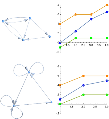
Figure 1. The Königsberg bridge graph considered by Leonhard Euler is a multi-graph. Removing the first row and column of the Kirchhoff matrix is the Kirchhoff matrix of a quiver with 3 vertices shown below. To the right one can see the eigenvalues sandwiched between lower and upper bound given in Theorem 1 and Theorem 2.

2.6.

Example. The Königsberg bridge graph

$$G=(\{1,2,3,4\},\{(12),(12),(14),(14),(23),(34)\})$$

is an early appearance of a multi-graph. Its Kirchhoff matrix is $K=\left[\begin{array}[]{cccc}4&-2&0&-2\\ -2&4&-1&-1\\ 0&-1&2&-1\\ -2&-1&-1&4\\ \end{array}\right]$. We have $d_{1}=2,d_{2}=d_{3}=d_{4}=4$ and $\lambda_{1}=0,\lambda_{2}=(9-\sqrt{17})/2,\lambda_{3}=5,\lambda_{4}=(9+\sqrt{17})/2$. The principal submatrix in which the first row and column are deleted has the eigenvalues $1,4,5$.

2.7.

Example. The Good-Will-Hunting multi-graph [36, 22]

$$G=(\{(1,2,3,4),\{(12),(24),(14),(23),(23)\})$$

was seen as a challenge on a chalk board in the 1997 coming-of-age movie “Good Will Hunting”. We have $K=B-A=\left[\begin{array}[]{cccc}2&-1&0&-1\\ -1&4&-2&-1\\ 0&-2&2&0\\ -1&-1&0&2\\ \end{array}\right]$. The first assignment in the Good-Will-Hunting problem was to write down the adjacency matrix $A$. We have $d_{1}=d_{2}=d_{3}=2,d_{4}=4$ and $\lambda_{1}=0,\lambda_{2}=(7-\sqrt{17})/2,\lambda_{3}=3,\lambda_{4}=(7+\sqrt{17})/2$. The principal sub-matrix in which the second row and column were deleted has eigenvalues $1,2,3$. It is the Kirchhoff matrix of the quiver $G=(\{(1,3,4),\{(14),(11),(44),(33),(33)\})$.

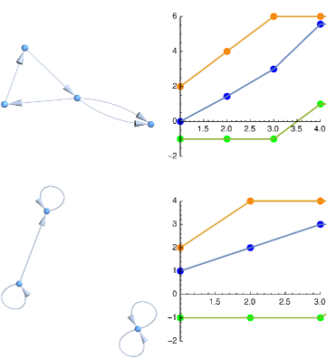
Figure 2. The picture shows the Good-Will-Hunting quiver and the principal sub-quiver obtained by deleting the vertex with maximal degree, snapping all its connections to loops on its neighbors. Again we see in each case the corresponding spectra, sandwiched between the upper and lower bounds given in Theorem 1 and Theorem 2.

3. Proofs

3.1.

Induction is enabled by the following observation.

Lemma 3.

Any principal submatrix of a Kirchhoff matrix of quiver with $2$ or more vertices is the Kirchhoff matrix of an quiver.

3.2.

For the lower bound, we will need the following observation:

Lemma 4.

Any principal submatrix of a Kirchhoff matrix of quiver without multiple connections with $2$ or more vertices is the Kirchhoff matrix of an quiver without multiple connections.

Proof.

Removing the row and column to a vertex $v$ has the effect that we look at the quiver with vertex set $V\setminus\{v\}$ for which $k$ additional loops have been added at every entry $w\in V\setminus\{v\}$ which had $k$ multiple connections to $v$ in the original graph $G$. We could also allow $n=1$ (in which case we have the $1\times 1$ matrix $K=[l]$ for a quiver with $l$ loops), but then the principal sub-matrix is the empty matrix which can be thought of as the Kirchhoff matrix of the empty graph. ∎

3.3.

A consequence is that the class of Kirchhoff matrices of quivers are a class of matrices which are invariant under the operation of taking principal sub-matrices. We should also note the obvious:

Lemma 5.

The Kirchhoff matrix of a quiver has non-negative spectrum.

Proof.

We use $K=F^{T}F$ and write $(v,w)$ for the dot product of two vectors $v,w$. If $Kv=\lambda v$ with unit eigenvector $v$, we have $\lambda=\lambda(v,v)=(\lambda v,v)=(Kv,v)=(F^{T}Fv,v)=(Fv,Fv)\geq 0$. ∎

3.4.

The proof of Theorem 1 and Theorem 2 are both by induction with respect to the number $n$ of vertices. The induction step uses the Cauchy interlace theorem (also called separation theorem) [21]: if $\mu_{k}$ are the eigenvalues of $\phi(K)$, then $\lambda_{k}\leq\mu_{k}\leq\lambda_{k+1}$. (The interlace theorem follows from the Hermite-Kakeya theorem for real polynomials [23, 14]. If $f$ is a monic polynomial of degree $n$ with real roots $\lambda_{1}\leq\cdots\leq\lambda_{n}$ and $g$ is a monic polynomial of degree $n-1$ with real roots $\mu_{1}\leq\cdots\leq\mu_{n-1}$ then $g$ interlaces $f$ if $\lambda_{1}\leq\mu_{1}\leq\lambda_{2}\leq\cdots\leq\mu_{n-1}\leq\lambda_{n}$.)

3.5.

Here is the proof of Theorem 1:

Proof.

The induction foundation $n=1$ works because the result holds for the Kirchhoff matrix of a quiver with $n=1$ vertices and $l$ loops. Indeed, this $1\times 1$ matrix $K=[l]$ has a non-negative entry $l$ and $\lambda_{1}=l$ and $d_{1}=l$.
Assume the claim is true for quivers with $n$ vertices. Take a quiver with $n+1$ vertices and let $K$ denote its Kirchhoff matrix. Pick the row with maximal diagonal entry and delete this row and column. This produces a Kirchhoff matrix $L$ of a quiver $H$ with $n$ vertices. By Cauchy interlacing, the eigenvalues $\mu_{k}$ of $L$ satisfy $0\leq\lambda_{1}\leq\mu_{1}\leq\cdots\leq\lambda_{n}\leq\mu_{n}\leq\lambda_{n+1}$. We know by induction that $\lambda_{k}\leq\mu_{k}\leq d_{k}+d_{k-1}$ for $1\leq k\leq n$. So, also $\lambda_{k}\leq\mu_{k}$ for $k\leq n$. The interlace theorem does not catch the largest eigenvalue $\lambda_{n+1}$. This requires an upper bound for the spectral radius. This is where Anderson and Morley [1] come in. They realized that $K=F^{*}F$ is essentially iso-spectral to $FF^{*}$. The later is the adjacency matrix of the line graph but with the modification that all diagonal entries are $2$ (for edges connecting two vertices) or $1$ (for loops). Since the row or column sum of $FF^{*}$ is bound by $d_{k}(a)+d_{k}(b)$ for any edge $(a,b)$, the upper bound holds. Having shown the Anderson-Morley for quivers gives also $\lambda_{n+1}\leq d_{n+1}+d_{n}$ for all quivers. ∎

3.6.

Here is the proof of Theorem 2:

Proof.

The induction foundation $n=1$ holds because every quiver without multiple connections satisfies $d_{1}\leq n-1$. This implies $0=\lambda_{1}\geq d_{1}-(n-1)$.
Assume the claim is true for all quivers with $n$ vertices. Take a quiver with $n+1$ vertices and let $K$ denote its Kirchhoff matrix. Pick the row with the minimal diagonal entry and delete this row and corresponding column. This is a Kirchhoff matrix $L$ of a quiver $H$ with $n$ vertices. By Cauchy interlacing and Lemma 2, the eigenvalues $\mu_{k}$ of $L$ satisfy $d_{1}-((n+1)-1)\leq\lambda_{1}\leq\mu_{1}\leq\cdots\leq\lambda_{n}\leq\mu_{n}\leq\lambda_{n+1}$. From this and induction we conclude $\lambda_{k}\geq\mu_{k-1}\geq d_{H,k-1}-(n_{H}-(k-1))$ for $k\geq 2$. But $d_{H,k-1}=d_{G,k}$ and $n_{H}=d_{G}-1$ so that $\lambda_{k}\geq d_{H,k-1}-(n_{H}-(k-1))=d_{G,k}-(n_{G}-1-(k-1))=d_{G,k}-(n_{G}-k)$ which needed to be shown. ∎

3.7.

Here is the proof of Lemma 1:

Proof.

The proof is the same than in the Anderson-Morley case, because we still have the super-symmetry situation allowing us to relate $K=F^{T}F$ with $K_{1}=FF^{T}$. The later is a $m\times m$ matrix which has $1$ in the diagonal if the edge had been a loop and $2$ in the diagonal where the edge connects two points. Furthermore $K_{1}(e,f)=-1$ or $1$. If we look at the $k$’th column belonging to an edge $e$, then the sum of the absolute values of the column entries is bound by $d_{n}+d_{n-1}$. The spectral radius $K_{1}$ is therefore bound by $d_{n}+d_{n-1}$. Since $K$ and $K_{1}$ have the same non-zero eigenvalues, also the spectral radius of $K$ is bound above by $d_{n}+d_{n-1}$. ∎

3.8.

Here is the proof of Lemma 2:

Proof.

We use induction with respect to the number $l$ of self-loops at the lowest degree vertex. The statement is true for graphs for $l=0$ loops, because there are then maximally $n-1$ neighboring vertices $d_{1}\leq n-1$ so that $d_{1}-(n-1)\leq 0$. The general statement $\lambda_{1}\geq 0$ proven above implies that if we have $l$ loops at the lowest degree vertex then $0\leq\lambda_{1}<d_{1}-(n-1)$. This means $d_{1}>n-1$ so that there are at least $q=d_{1}-(n-1)>0$ loops at this vertex. Because $d_{k}-(n-1)\geq d_{1}-(n-1)$ there are also at least $q$ loops at every other vertex. Removing one loop at every vertex lowers all eigenvalues by $1$ and all $d_{k}$ by $1$ and $l$ by $1$. We get a quiver with $l-1$ loops at the lowest vertex degree vertex, where still $d_{1}-(n-1)>\lambda_{1}$. This is satisfied because the induction assumption was $d_{1}-(n-1)\leq\lambda_{1}$ for all quivers with $l-1$ or less loops at the lowest degree vertex. ∎

4. Remarks

4.1.

One could look also the Schrödinger case $L=K+V$, where $V$ is a diagonal matrix containing non-negative potential values $V_{k}$. More generally, we can use magnetic operators $Lu(v)=(Ku)(v)+V(v)u(v)-\sum_{(v,w)\in E}W(w)$ with $W(w)\geq 0$ and $V(v)\geq 0$. If $V_{k},W_{k}\in\mathbb{N}$, we have a situation which is covered by quivers. [12] uses the term “differential operator” or “operator with magnetic field”.

4.2.

Technically, we are bound to non-negative potentials $V,W$ but a scaling of $L$ allows to cover rational valued potentials and by a limiting procedure also real cases, at least for the upper bound. It is illustrative to track an eigenvalue $\lambda$ with eigenvector $v$ is changed if a diagonal entry $V_{k}$ is varied which is a rank one perturbation. The first Hadamard deformation formula gives $\lambda(t)^{\prime}=v_{k}^{2}\geq 0$. The second Hadamard deformation formula gets $\lambda(t)^{\prime\prime}>0$ depending on the other eigenvalues illustrating eigenvalue repulsion. Increasing $V$ or increasing $W$ both can only increase all eigenvalues.

Corollary 1 (Schroedinger estimate).

If $L=K+V-W$ where $K$ is the Kirchhoff Laplacian of a quiver and $V,W$ are non-negative functions then $\lambda_{k}\leq d_{k}+d_{k-1}$, where $d_{k}$ are the diagonal entries of $L$.

4.3.

Similarly than the Schur-Horn inequality $\sum_{j=1}^{k}\lambda_{j}\leq\sum_{j=1}^{k}d_{j}$ which is true for any symmetric matrix with diagonal entries $d_{j}$, Theorem (1) controls how close the ordered eigenvalue sequence is to the ordered vertex degree sequence. But Theorem (1) has a different nature than Schur-Horn: for example, if the eigenvalues increase exponentially like $\lambda_{k}=6^{k}$, then the inequality $\lambda_{k}\leq 2d_{k}$ implies on a logarithmic scale $\log(\lambda_{k})\leq\log(2)+\log(d_{k})$. Schur-Horn does not provide that. Also the Gershgorin circle theorem would only establish $\log(\lambda)\leq\log(2)+\log(d_{n})$, where $d_{n}$ is the largest entry, because that theorem assures only that in each Gershgorin circle, there is at least one eigenvalue.

4.4.

Anderson and Morley [1] already had the better bound $\max_{(x,y)\in E}d(x)+d(y)$ and Theorem (1) could be improved in that $d_{k}+d_{k-1}$ could be replaced by ${\rm max}_{(x,y)\in E}d_{k}+d_{j}$. Any general better upper bound of the spectral radius would lead to sharper results. The Anderson-Morley estimate as an early use of a McKean-Singer super symmetry [34] (see [24] for graphs), in a simple case, where one has only $0$-forms and $1$-forms. There, it reduces to the statement that $K=F^{*}F$ is essentially isospectral to $FF^{*}$ which is true for all matrices. It uses that the Laplacian $K$ is of the form $F^{*}F={\rm div}{\rm grad}$, where $F={\rm grad}$ is the incidence matrix $Ff((a,b))=f(b)-f(a)$ for functions $f$ on vertices (0-forms) leading to functions on oriented edges (1-form).

4.5.

Much effort has gone into estimating the spectral radius of the Kirchhoff Laplacian. It is bounded above by the spectral radius of the sign-less Kirchhoff Laplacian $|K|$ in which one takes the absolute values for each entry. This matrix is a non-negative matrix in the connected case has a power $|K|^{n}$ with all positive entries so that by the Perron-Frobenius theorem, the maximal eigenvalue is unique. (The Kirchhoff matrix itself of course can have multiple maximal eigenvalues like for the case of the complete graph). Also, unlike $K$ which is never invertible, $|K|$ is can be invertible if $G$ is not bipartite. If we treat a graph as a one-dimensional simplicial complex (ignoring 2 and higher dimensional simplices in the graph), and denote b $d$ the exterior derivative of this skeleton complex, then $(d+d^{*})^{2}=K_{0}+K_{1}$ where $K=K_{0}=d^{*}d$ is the Kirchhoff matrix and $K_{1}=dd^{*}$ is the one-form matrix with the same spectral radius, leading to [1]. Much work has gone in improving this [7, 42, 33, 47, 13, 40, 31]. We have used that an identity coming from connection matrices [29].

4.6.

We stumbled on the theorem when looking for bounds on the tail distribution $\mu([x,\infty))$ of the limiting density of states $\mu$ of the Barycentric limit $\lim_{n\to\infty}G_{n}$ of a finite simple graph $G=G_{0}$, where $G_{n}$ is the Barycentric refinement of $G_{n-1}$ in which the complete sub-graphs of $G_{n-1}$ are the vertices and two such vertices are connected if one is contained in the other [27, 28]. We wanted a potential $U(z)=\int_{0}^{\infty}\log(z-w)\;d\mu(w)$ because $U(-1)$ measures the exponential growth of rooted spanning forests while $U(0)$ captures the exponential growth of the rooted spanning trees.

4.7.

The connection is that in general, the pseudo determinant [26] ${\rm Det}(K)=\prod_{\lambda\neq 0}\lambda$ is the number of rooted spanning trees in $G$ by the Kirchhoff matrix tree theorem and ${\rm det}(1+K)$ is the number of rooted spanning forests in $G$ by the Chebotarev-Shamis matrix forest theorem [35, 37, 25]. All these relations follow directly from the generalized Cauchy-Binet theorem that states that for any $n\times m$ matrices $F,G$, one has the pseudo determinant version ${\rm Det}(F^{T}G)=\sum_{|P|=k}\det(F_{P})\det(G_{P})$ with $k$ depends on $F,G$ and $\det(1+xF^{T}G)=\sum_{P}x^{|P|}\det(F_{P})\det(G_{P})$. Pythagorean identities like ${\rm Det}(F^{T}F)=\sum_{|P|=k}\det^{2}(F_{P})$ and $\det(1+F^{T}F)=\sum_{P}\det^{2}(F_{P})$ follow for an arbitrary $n\times m$ matrix $F$. Applied to the incidence matrix $F$ of a connected graph, where $k(A)=n-1$ is the rank of $K=F^{T}F$, the first identity counts on the right spanning trees and the second identity counts on the right the number of spanning forests.

4.8.

Having noticed that the tree-forest ratio $\tau(G)={\rm Det}(1+K)/{\rm Det}(K)=\prod_{\lambda\neq 0}(1+1/\lambda)$ has a Barycentric limit $\lim_{n\to\infty}(1/|G_{n}|)\log(\tau(G_{n}))$, we interpreted this as $U(-1)-U(0)$ requiring the normalized potential to exist. By the way, for complete graphs $G=K_{n}$ the tree-forest ratio is $(1+1/n)^{n-1}$ and converges to the Euler number $e$. For triangle-free graphs, $\log(\tau(G_{n}))/|V(G_{n})|$ converges to $\log(\phi^{2})$, where $\phi=(1+\sqrt{5})/2$ is the golden ratio. For example, for $G=C_{n}$, where ${\rm Det}(K)=n^{2}$ and the number of rooted spanning forests is the alternate Lucas number recursively defined by $L(n+1)=3L(n)-L(n-1)+2,L(0)=0,L(1)=1$. We proved in general that $\log(\tau(G_{n}))/|V(G_{n}))|$ converges under Barycentric refinements $G_{0}\to G_{1}\to G_{2}\dots$ for arbitrary graphs to a universal constant that only depends on the maximal dimension of $G=G_{0}$.

4.9.

Theorem (1) needs to be placed into the context of the spectral graph literature like [4, 12, 16, 6, 9, 10, 41] or articles like [20, 43, 39]. Most research work in this area has focused on small eigenvalues, like $\lambda_{2}$ or large eigenvalues, like the spectral radius $\lambda_{n}$. For $\lambda_{2}$, there is a Cheeger estimate $h^{2}/(2d_{n})\leq\lambda_{2}\leq h$ for the eigenvalue $\lambda_{2}$ and Cheeger constant $h=h(G)$ [8] first defined for Riemannian manifolds, meaning in the graph case that one needs remove $h|H|$ edges to separate a sub-graph $H$ from $G$ (see [12]). For the largest eigenvalue $\lambda_{n}$, the Anderson-Morley bound has produced an industry of results.

4.10.

Let us look at some example. Figure (1) shows more visually what happens in some examples of graphs with $n=10$ vertices.
a) For the cyclic graph $C_{4}$, the Kirchhoff eigenvalues are $\lambda_{1}=0,\lambda_{2}=2,\lambda_{3}=2,\lambda_{4}=4$ and the edge degrees are $d_{1}=d_{2}=d_{3}=d_{4}=2$.
b) For the star graph with $n-1$ spikes, the eigenvalues are $\lambda_{1}=0,\lambda_{2}=\cdots\lambda_{n-1}=1,\lambda_{n}=n$ while the degree sequence is $d_{1}=\cdots=d_{n-1}=1,d_{n}=n$.
c) For a complete bipartite graph $K_{n,m}$ with $m\leq m$, we have $0\leq m\leq\cdots\leq m\leq n\cdots\leq n$ with $m-1$ eigenvalues $m$ and $n-1$ eigenvalues $n$. The degree sequence has $m\leq m\leq\cdots\leq m\leq n\leq\cdots\leq n$ with $m$ entries $m$ and $n$ entries $n$.

4.11.

From all the $38$ isomorphism classes of connected graphs with $4$ vertices, there are only $3$, for which equality holds in Theorem (1) and $7$ for which $\lambda_{k}=2d_{k}$. From the $728$ isomorphism classes of connected graphs with $5$ vertices, there are none for Theorem (1) and $5$ for $\lambda_{k}=2d_{k}$. From the $26704$ isomorphism classes of connected graphs with $6$ vertices, there are $70$ for which Theorem (1) has equality and $76$ for which $\lambda_{k}=2d_{k}$. It is always only the largest eigenvalue, where we have seen equality $\lambda_{n}=2d_{n}$ to hold.

4.12.

The theorem implies $\sum_{j=1}^{k}\lambda_{j}\leq 2\sum_{j=1}^{k}d_{j}$ which is weaker than the Schur-Horn inequality $\sum_{j=1}^{k}\lambda_{j}\leq\sum_{j=1}^{k}d_{j}$. The later result is of wide interest. It can be seen in the context of partial traces [44] $\sum_{j=1}^{k}\lambda_{j}={\rm inf}_{dim(V)=k}{\rm tr}(A|V)$ and is special case of the Atiyah-Guillemin-Sternberg convexity theorem [2, 18]. The Schur inequality has been sharpened a bit for Kirchhoff matrices to $\sum_{j=1}^{k}\lambda_{j}\leq\sum_{j=1}^{k}d_{j}-1$ [6] Proposition 3.10.1.

4.13.

Unlike the Schur-Horn inequality, Theorem (1) does not extend to general symmetric matrices. Already for $A=\left[\begin{array}[]{cc}1&3\\ 3&1\end{array}\right]$ which has eigenvalues $\lambda_{1}=-2,\lambda_{2}=4$ and with $d_{1}=1,d_{2}=1$, the inequality $\lambda_{2}\leq 2d_{2}$ fails. It also does not extend to symmetric matrices with non-negative eigenvalues, but also this does not work as $A=\left[\begin{array}[]{ccc}1&1&1\\ 1&1&1\\ 1&1&1\end{array}\right]$ shows, as this matrix has eigenvalues $0,0,3$ and diagonal entries $1,1,1$. The case of $n\times n$ matrices with constant entries $1$ is an example with eigenvalues $0$ and $n$ showing that no estimate $\lambda_{n}\leq Cd_{n}$ is in general possible for symmetric matrices even when asking the diagonal entry to dominate the other entries.

5. Open ends

5.1.

Theorem (1) would also follow from the statement

(1) $$\sum_{j=1}^{k}d_{j}-\sum_{j=1}^{k}\lambda_{j}\leq d_{k}$$

which would be of independent interest as it estimates the Schur-Horn error. Indeed, Schur-Horn gives together with such a hypothetical error bound $0\leq\sum_{j=1}^{k}d_{j}-\sum_{j=1}^{k}\lambda_{j}+(d_{k+1}-\lambda_{k+1})\leq d_{k}+(d_{k+1}-\lambda_{k+1})$ for all $k$, which is equivalent to $\lambda_{k}\leq d_{k}+d_{k-1}$ for all $k$. Can we prove the above Schur-Horn error estimate (1)? We do not know yet but our experiments indicate:

Conjecture A: [Schur-Horn error] Estimate (1) holds for all finite simple graphs.

5.2.

The Brouwer-Haemers bound $\lambda_{k}\geq d_{k}-(n-k)+1$ is very good for large $k$ but far from optimal for smaller $k$, especially if $n$ is large. The guess $d_{k-1}/2\leq\lambda_{k}$ assuming $d_{-1}=0$ is only a rule of thumb, as it seems fails only in rare cases. The next thing to try is $d_{k-2}/2\leq\lambda_{k}$ and this is still wrong in general but there are even less counter examples. We can try $d_{k-2}/3$ for which we have not found a counter example yet but it might just need to look for larger networks to find a counter example. We still believe that there is an affine lower bound. This is based only on limited experiments like for $A=1/3$ where it already looks good. The case $B=0$ could well occur in our assessment so far but it is safer to include also a constant..

Conjecture B: [Affine Brouwer-Haemers bound] There exist constants $0<A<1$ and $B$ such that for all graphs and $1\leq k\leq n$ we have $Ad_{k}-B\leq\lambda_{k}$.

5.3.

We see for many Erdös-Rényi graphs that an upper bound $\lambda_{k}\leq Cd_{k}$ holds for most graphs for any $C>1$, if the graphs are large. A possible conjecture is that

Conjecture C: [Linear bound for Erdoes-Renyi] For all $C>1$ and all $p\in[0,1]$, the probability of the set of graphs in the Erdös-Rényi probability space $E(n,p)$ with $\lambda_{k}\leq Cd_{k}$ for all $1\leq k\leq n$ goes to $1$ for $n\to\infty$.

5.4.

The lower Brouwer-Haemers bound for graphs has for $k=1$ the exception $K_{n}$, the complete graph. For $n=1$ with $d_{1}$ loops, we have $K=[d_{1}]$ and so $\lambda_{1}=d_{1}$. The modified Brouwer-Haemers bound $\lambda_{1}\geq d_{1}-(n-1)$ does not hold for all quivers but requires no multiple connections. We believe that the original Brouwer-Haemers bound could hold for every non-magnetic quiver and all $k\geq 2$, similarly as in the graph case, where $k=1$ was an exception. But now, we can not apply the simple induction proof because the left bound for $\lambda_{1}$ is not universally valid. Also the following is only based on small experiments so far:

Conjecture D: [Brouwer-Haemers for non-magnetic quivers]

$$\lambda_{k}\geq d_{k}-(n-k)+1\;$$

holds for all $k\geq 2$.

5.5.

Theorem 2 gives only $\lambda_{k}\geq d_{k}-(n-k)$ but holds for all $k\geq 1$ and not only for $k\geq 2$.

6. Illustration

6.1.

Here are a few examples of spectra with known upper and lower bounds:

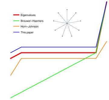
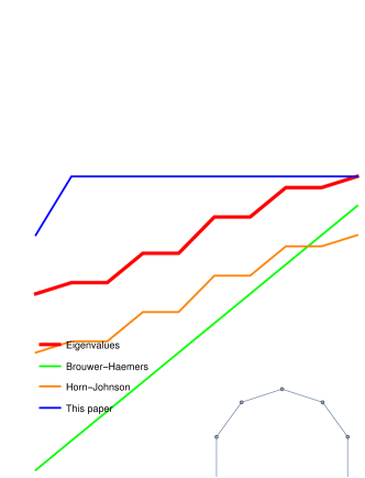
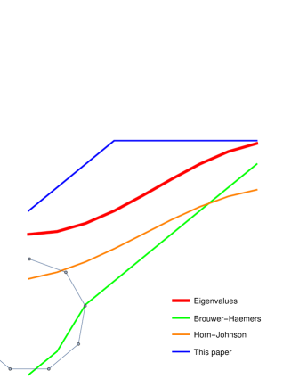
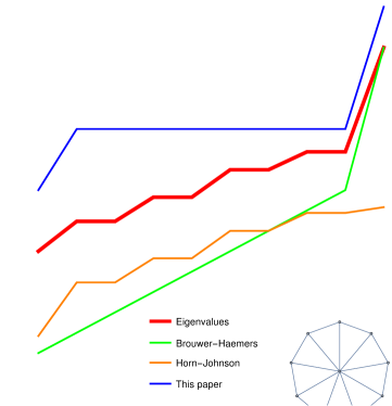
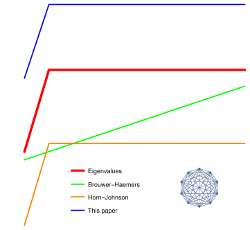
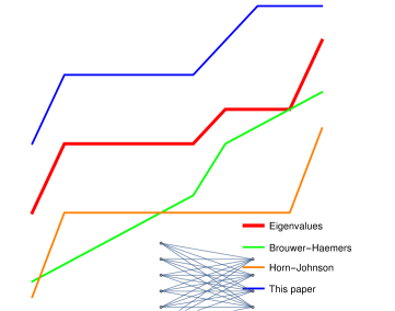
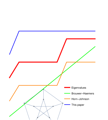
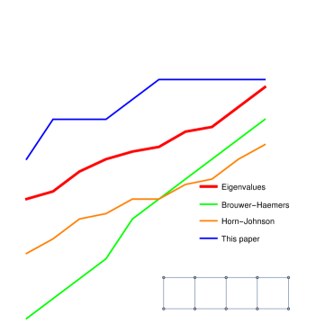
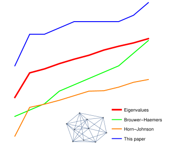
Figure 3. This figure shows examples of spectra of simple graphs and compares them with known upper and lower bounds. We see first the Star, Cycle and Path graph, then the Wheel, Complete, Bipartite graph, and finally the Petersen, Grid and Random graph, all with $10$ vertices. The eigenvalues are outlined thick (in red). Above we see the upper bound (in blue) as proven in the present paper. Then there are the Brouwer-Haemers and Horn-Johnson lower bounds which, as the examples show, do not always compete but complement each other.

References

- [1] W.N. Anderson and T.D. Morley. Eigenvalues of the Laplacian of a graph. Linear and Multilinear Algebra, 18(2):141–145, 1985.
- [2] M. Atiyah. Convexity and commuting Hamiltonians. Bull. London Math. Soc, 14:1–15, 1982.
- [3] M. Baker and S. Norine. Riemann-Roch and Abel-Jacobi theory on a finite graph. Advances in Mathematics, 215:766–788, 2007.
- [4] N. Biggs. Algebraic Graph Theory. Cambridge University Press, 1974.
- [5] A.E. Brouwer and H.H Haemers. A lower bound for the Laplacian eigenvalues of a graph - proof of a conjecture by guo. Lin. Alg. Appl., 429:2131–2135, 2008.
- [6] A.E. Brouwer and W.H. Haemers. Spectra of graphs. Springer, 2012.
- [7] R. A. Brualdi and A. J. Hoffmann. On the spectral radius of (0,1)-matrices. Linear Algebra and its Applications, 65:133–146, 1985.
- [8] J. Cheeger. A lower bound for the smallest eigenvalue of the Laplacian. In R. Gunning, editor, Problems in Analysis, 1970.
- [9] F. Chung. Spectral graph theory, volume 92 of CBMS Reg. Conf. Ser. AMS, 1997.
- [10] M. Doob D. Cvetković and H. Sachs. Spectra of graphs. Johann Ambrosius Barth, Heidelberg, third edition, 1995. Theory and applications.
- [11] K.Ch. Das. The Laplacian spectrum of a graph. Comput. Math. Appl., 48(5-6):715–724, 2004.
- [12] Y.Colin de Verdière. Spectres de Graphes. Sociéte Mathématique de France, 1998.
- [13] L. Feng, Q. Li, and X-D. Zhang. Some sharp upper bounds on the spectral radius of graphs. Taiwanese J. Math., 11(4):989–997, 2007.
- [14] S. Fisk. A very short proof of Cauchy’s interlace theorem for eigenvalues of Hermitian matrices. https://arxiv.org/abs/math/0502408, 2005.
- [15] S. Gershgorin. Über die Abgrenzung der Eigenwerte einer Matrix. Bulletin de l’Academie des Sciences de l’URSS, 6:749–754, 1931.
- [16] C. Godsil and G. Royle. Algebraic Graph Theory. Springer Verlag, 2001.
- [17] R. Grone and R. Merris. The Laplacian spectrum of a graph. II. SIAM J. Discrete Math., 7(2):221–229, 1994.
- [18] V. Guillemin and S. Sternberg. Convexity properties of the moment mapping. Invent. Math, 67:491–513, 1982.
- [19] J-M. Guo. On the third largest Laplacian eigenvalue of a graph. Linear and Multilinear Algebra, 55:93–102, 2007.
- [20] Ji-Ming Guo. A new upper bound for the Laplacian spectral radius of graphs. Linear Algebra and its Applications, 400:61–66, 2005.
- [21] R.A. Horn and C.R. Johnson. Matrix Analysis. Cambridge University Press, second edition edition, 2012.
- [22] G. Horvath and C.A. Szabo J. Korandi. Mathematics in good will hunting ii: problems from the students perspective. Education, Mathematics Teaching Mathematics and Computer Science, 2013.
- [23] S-G. Hwang. Cauchy’s Interlace Theorem for Eigenvalues of Hermitian Matrices. American Mathematical Monthly, 111, 2004.
-
[24]
O. Knill.
The McKean-Singer Formula in Graph Theory.
http://arxiv.org/abs/1301.1408, 2012. -
[25]
O. Knill.
Counting rooted forests in a network.
http://arxiv.org/abs/1307.3810, 2013. - [26] O. Knill. Cauchy-Binet for pseudo-determinants. Linear Algebra Appl., 459:522–547, 2014.
-
[27]
O. Knill.
The graph spectrum of barycentric refinements.
http://arxiv.org/abs/1508.02027, 2015. -
[28]
O. Knill.
Universality for Barycentric subdivision.
http://arxiv.org/abs/1509.06092, 2015. -
[29]
O. Knill.
The Hydrogen identity for Laplacians.
https://arxiv.org/abs/1803.01464, 2018. - [30] J. Li, W.C. Shiu, and W.H. Chan. The Laplacian spectral radius of some graphs. Linear algebra and its applications, pages 99–103, 2009.
- [31] J. Li, W.C. Shiu, and W.H. Chan. The Laplacian spectral radius of graphs. Czechoslovak Mathematical Journal, 60:835–847, 2010.
- [32] J-S Li and Y-L. Pan. A note on the second largest eigenvalue of the Laplacian matrix of a graph. Linear and Multilinear Algebra, 48, 2000.
- [33] J.S. Li and X.D. Zhang. A new upper bound for eigenvalues of the Laplacian matrix of a graph. Linear Algebra and Applications, 265:93–100, 1997.
- [34] H.P. McKean and I.M. Singer. Curvature and the eigenvalues of the Laplacian. J. Differential Geometry, 1(1):43–69, 1967.
- [35] P.Chebotarev and E. Shamis. Matrix forest theorems. arXiv:0602575, 2006.
- [36] B. Polster and M. Ross. Math Goes to the Movies. Johns Hopkins University Press, 2012.
- [37] E.V. Shamis P.Yu, Chebotarev. A matrix forest theorem and the measurement of relations in small social groups. Avtomat. i Telemekh., 9:125–137, 1997.
- [38] R. Merris R. Grone and V.S. Sunder. The Laplacian spectrum of a graph. SIAM J. Matrix Anal. Appl., 11(2):218–238, 1990.
- [39] R. Merris R. Grone and V.S. Sunder. The Laplacian spectrum of a graph. Siam J. Matrix Anal. Appl., 11:218–238, 1990.
- [40] L. Shi. Bounds of the Laplacian spectral radius of graphs. Linear algebra and its applications, pages 755–770, 2007.
- [41] D.A. Spielman. Spectral graph theory. lecture notes, 2009.
- [42] R. P. Stanley. A bound on the spectral radius of graphs. Linear Algebra and its Applications, 87:267–269, 1987.
- [43] T. Stephen. A majorization bound for the eigenvalues of some graph Laplacians. SIAM Journal on Discrete Mathematics, 21:303–312, 2007.
- [44] T. Tao. Eigenvalues and sums of Hermitian matrices. https://terrytao.wordpress.com/tag/schur-horn-inequalities/, 2010.
- [45] N. Trinajstic. Chemical Graph Theory. Mathematical chemistry series. CRC Press, 2 edition, 1992.
- [46] R.S. Varga. Gershgorin and His Circles. Springer Series in Computational Mathematics 36. Springer, 2004.
- [47] Xiao-Dong Zhang. Two sharp upper bounds for the Laplacian eigenvalues. Linear Algebra and Applications, 376:207–213, 2004.
- [48] H. Zhou and X. Xu. Sharp upper bounds for the Laplacian spectral radius of graphs. Mathematical Problems in Engineering, 2013, 2013.