From Width-Based Model Checking to
Width-Based Automated Theorem Proving

Abstract

In the field of parameterized complexity theory, the study of graph width measures has been intimately connected with the development of width-based model checking algorithms for combinatorial properties on graphs. In this work, we introduce a general framework to convert a large class of width-based model-checking algorithms into algorithms that can be used to test the validity of graph-theoretic conjectures on classes of graphs of bounded width. Our framework is modular and can be applied with respect to several well-studied width measures for graphs, including treewidth and cliquewidth.

As a quantitative application of our framework, we show that for several long-standing graph-theoretic conjectures, there exists an algorithm that takes a number $k$ as input and correctly determines in time double-exponential in $k^{O(1)}$ whether the conjecture is valid on all graphs of treewidth at most $k$. This improves significantly on upper bounds obtained using previously available techniques.

Keywords: Dynamic Programming Cores, Width Measures, Automated Theorem Proving

1 Introduction

1.1 Motivation

When mathematicians are not able to solve a conjecture about a given class of mathematical objects, it is natural to try to test the validity of the conjecture on a smaller, or better behaved class of objects. In the realm of graph theory, a common approach is to try analyze the conjecture on restricted classes of graphs, defined by fixing some structural parameter. In this work, we push forward this approach from a computational perspective by focusing on parameters derived from graph width measures. Prominent examples of such parameters are the treewidth of a graph, which intuitively quantifies how much a graph is similar to a tree [70, 10, 42] and the cliquewidth of a graph, which intuitively quantifies how much a graph is similar to a clique [32]. More specifically, we are concerned with the following problem.

Problem 1 (Width-Based ATP).

Given a graph property $\mathbb{P}$ and a positive integer $k$, is it the case that every graph of width at most $k$ belongs to $\mathbb{P}$?

Problem 1 provides a width-based approach to the field of automated theorem proving (ATP). For instance, consider Tutte’s celebrated $5$-flow conjecture [77], which states that every bridgeless graph has a nowhere-zero $5$-flow. Let HasBridge be the set of all graphs that have a bridge, and $\texttt{NZFlow}(5)$ be the set of all graphs that admit a nowhere-zero $5$-flow. Then, proving Tutte’s $5$-flow conjecture is equivalent to showing that every graph belongs to the graph property $\texttt{HasBridge}\vee\texttt{NZFlow}(5)$. Since Tutte’s conjecture has been unresolved for many decades, one possible approach for gaining understanding about the conjecture is to try to determine, for gradually increasing values of $k$, whether every graph of width at most $k$, with respect to some fixed width-measure, belongs to $\texttt{HasBridge}\vee\texttt{NZFlow}(5)$. What makes this kind of question interesting from a proof theoretic point of view is that several important classes of graphs have small width with respect to some width measure. For instance, trees and forests have treewidth at most $1$, series-parallel graphs and outerplanar graphs have treewidth at most $2$, $k$-outerplanar graphs have treewidth at most $3k-1$, co-graphs have cliquewidth at most $2$, any distance hereditary graph has cliquewidth $3$, etc [11, 14, 21, 17, 16, 47]. Therefore, proving the validity of a given conjecture on classes of graphs of small width corresponds to proving the conjecture on interesting classes of graphs.

1.2 Our Results

In this work, we introduce a general and modular framework that allows one to convert width-based dynamic programming algorithms for the model checking of graph properties into algorithms that can be used to address Problem 1. More specifically, our main contributions are threefold.

1. We start by defining the notions of a treelike decomposition class (Definition 2) and of a treelike width-measure (Definition 3). These two notions can be used to express several classic, well studied width measures for graphs, such as treewidth [13], pathwidth [54], carving width [76], cutwidth [24, 75], bandwidth [24], cliquewidth [32], etc, and some more recent measures such as ODD width [4].

2. Subsequently, we introduce the notion of a treelike dynamic programming core (Definition 8), a formalism for the specification of dynamic programming algorithms operating on treelike decompositions. As stand-alone objects, DP-cores are essentially a formalism for the specification of sets of terms, much like tree automata, but with the exception that transitions are specified implicitly, using functions. Nevertheless, when associated with the notion of a treelike decomposition class, DP-cores can be used to define classes of graphs. Furthermore, when satisfying a property called coherency (Definition 11), treelike DP-cores can be safely used for the purpose of model checking. Intuitively, coherency is a condition that requires that a DP-core gives the same answer when processing any two treelike decompositions of the same graph. Finally, our formalism is symbolic, in the sense that graphs are encoded as terms over a finite alphabet. This makes our approach suitable for the consideration of questions pertaining to the realm of automated theorem proving, as described next.

3. Intuitively, our main result (Theorem 33) states that if a graph property $\mathbb{P}$ is a dynamic combination (see Definition 30) of graph properties $\mathbb{P}_{1},\dots,\mathbb{P}_{\ell}$ that can be decided by coherent DP-cores $\mathsf{D}_{1},\mathsf{D}_{2},\dots,\mathsf{D}_{\ell}$ satisfying certain finiteness conditions, then the process of determining whether every graph of width at most $k$ belongs to $\mathbb{P}$ can be decided roughly in time

   $$2^{O(\beta(k)\cdot\mu(k))}\leq 2^{2^{O(\beta(k))})},$$

   where $\mu(k)$ and $\beta(k)$ are respectively the maximum multiplicity and the maximum bitlength of a DP-core from the list $\mathsf{D}_{1},\dots,\mathsf{D}_{\ell}$ (see Definition 14). Additionally, if a counterexample of width at most $k$ exists, then a term term of height at most $2^{O(\beta(k)\cdot\mu(k))}$ representing such a counterexample can be constructed (Corollary 28).

The modularity of our approach makes it highly suitable to be applied in the context of automated theorem proving. For instance, when specialized to the context of treewidth, our approach can be used to infer that several long-standing conjectures in graph theory can be tested on the class of graphs of treewidth at most $k$ in time double exponential in $k^{O(1)}$. Examples of such conjectures include Hadwiger conjecture [41], Tutte’s flow conjectures [77], Barnette’s conjecture [78], and many others (Section 6).

1.3 Related Work

General automata-theoretic frameworks for the development of dynamic programming algorithms have been introduced under a wide variety of contexts [40, 64, 65, 56, 66, 60, 57, 6, 7, 8]. In most of these contexts, automata are used to encode the space of solutions of combinatorial problems when a graph $G$ is given at the input. For instance, given a tree decomposition of width $k$ of a graph $G$, one can construct a tree automaton representing the set of proper $3$-colorings of $G$ [7].

In our framework, treelike DP-cores are used to represent families of graphs satisfying a given property. For instance, one can define a treelike DP-core $\mathsf{D}$, where for each $k\in\mathbb{N}$, $\mathsf{D}[k]$ is a finite representation of the set of all graphs of treewidth at most $k$ that are $3$-colorable. In our context it is essential that graphs of width $k$ are encoded as terms over a finite alphabet whose size only depends on $k$. We note that the idea of representing families of graphs as tree languages over a finite alphabets has been used in a wide variety of contexts [18, 2, 31, 37, 39, 30]. Nevertheless, the formalisms arising in these contexts are usually designed to be compatible with logical algorithmic meta-theorems, and for this reason, tree automata are meant to be compiled from logical specifications, rather than to be programmed. In contrast, we provide a framework that allows one to easily program state-of-the-art dynamic programming algorithms operating on treelike decompositions (see Section 5.3), and to safely combine these algorithms (just like plugins) for the purpose of width-based automated theorem proving.

The monadic second-order logic of graphs (MSO₂ logic) extends first-order logic by introducing quantification over sets of vertices and over sets of edges. This logic is powerful enough to express several well studied graph-theoretic properties such as connectivity, Hamiltonicity, $3$-colorability, and many others. Given that for each $k\in\mathbb{N}$, the MSO₂ theory of graphs of treewidth at most $k$ is decidable [73, 28], we have that if a graph property $\mathbb{P}$ is definable in MSO₂ logic, then there is an algorithm that takes an integer $k$ as input, and correctly determines whether every graph of treewidth at most $k$ belongs to $\mathbb{P}$. A similar result can be proved with respect to graphs of constant cliquewidth using MSO₁ logic [73], and for graphs of bounded ODD width using FO logic [4].

One issue with addressing Problem 1 using the logic approach mentioned above is that algorithms obtained in this way are usually based quantifier-elimination. As a consequence, the function upper-bounding the running time of these algorithms in terms of the width parameter grows as a tower of exponentials whose height depends on the number of quantifier alternations of the logical sentence given as input to the algorithm. For instance, the algorithm obtained using this approach to test the validity of Hadwiger’s conjecture restricted to $c$ colors on graphs of treewidth at most $k$ has a very large dependency on the width parameter. In [51], the time necessary to perform this task was estimated in $f(c,k)\leq p^{p^{p^{p}}}$, where $p=(k+1)^{(c-1)}$ [51]. Our approach yields a much smaller upper bound of the form $2^{2^{O(k\cdot\log k+c^{2})}}$. Significant reductions in complexity can also be observed for other conjectures.

Courcelle’s model checking theorem and its subsequent variants [29, 5, 20] have had a significant impact in the development of width-based model checking algorithms. Indeed, once a graph property has been shown to be decidable in FPT time using the machinery surrounding Courcelle’s theorem, the next relevant question is how small can the dependency in the width parameter be. Algorithms with optimal dependency on the width parameter have been obtained for a large number of graph properties [58, 67] under standard complexity theoretic assumptions, such as the exponential time hypothesis (ETH) [46, 45] and related conjectures [22, 23]. It is worth noting that in many cases, the development of such optimal algorithms requires the use of advanced techniques borrowed from diverse subfields of mathematics, such as structural graph theory [71, 9], algebra [79, 15, 61], combinatorics [68, 59], etc. Our framework allows one to incorporate several of these techniques in the development of faster algorithms for width-based automated theorem proving.

2 Preliminaries

We let $\mathbb{N}$ denote the set of natural numbers and $\mathbb{N}_{+}$ denote the set of positive natural numbers. We let $[0]~{}\dot{=}~{}\emptyset$, and for each $n\in\mathbb{N}_{+}$, we define $[n]~{}\dot{=}~{}\{1,...,n\}$. Given a set $S$, the set of finite subsets of $S$ is denoted by $\mathcal{P}_{\mathrm{fin}}(S)$.

In this work, a graph is a triple $G=(V,E,\rho)$ where $V\subseteq\mathbb{N}$ is a finite set of vertices, $E\subseteq\mathbb{N}$ is a finite set edges, and $\rho\subseteq E\times V$ is an incidence relation. For each edge $e\in E$, we let $\mathrm{endpts}(e)=\{v\in V\;:\;(e,v)\in\rho\}$ be the set of vertices incident with $e$. In what follows, we may write $V_{G}$, $E_{G}$ and $\rho_{G}$ to denote the sets $V$, $E$ and $\rho$ respectively. We let $|G|=|V_{G}|+|E_{G}|$ be the size of $G$. We let Graphs denote the set of all graphs. For us, the empty graph is the graph $(\emptyset,\emptyset,\emptyset)$ with no vertices, no edges, and no incidence pairs.

An isomorphism from a graph $G$ to a graph $H$ is a pair $\phi=(\phi_{1},\phi_{2})$ where $\phi_{1}:V_{G}\rightarrow V_{H}$ is a bijection from the vertices of $G$ to the vertices of $H$ and $\phi_{2}:E_{G}\rightarrow E_{H}$ is a bijection from the edges of $G$ to the edges of $H$ with the property that for each vertex $v\in V_{G}$ and each edge $e\in E_{G}$, $(v,e)\in\rho_{G}$ if and only if $(\phi_{1}(v),\phi_{2}(e))\in\rho_{H}$. If such a bijection exists, we say that $G$ and $H$ are isomorphic, and denote this fact by $G\sim H$.

A graph property is any subset $\mathbb{P}\subseteq\textsc{Graphs}$ closed under isomorphisms. That is to say, for each two isomorphic graphs $G$ and $H$ in Graphs, $G\in\mathbb{P}$ if and only if $H\in\mathbb{P}$. Note that the sets $\emptyset$ and Graphs are graph properties. Given a set $S$ of graphs, the isomorphism closure of $S$ is defined as the set $\mathsf{ISO}(S)=\{G\in\textsc{Graphs}\;:\;\exists H\in S,G\sim H\}.$

Given a graph property $\mathbb{P}$, a $\mathbb{P}$-invariant is a function $\mathcal{I}:\mathbb{P}\rightarrow S$, for some set $S$, that is invariant under graph isomorphisms. More precisely, $\mathcal{I}(G)=\mathcal{I}(H)$ for each two isomorphic graphs $G$ and $H$ in $\mathbb{P}$. If $\mathbb{P}=\textsc{Graphs}$, we may say that $\mathcal{I}$ is simply a graph invariant. For instance, chromatic number, clique number, dominating number, etc., as well as width measures such as treewidth and cliquewidth, are all graph invariants. In this work the set $S$ will be typically $\mathbb{N}$, when considering width measures, or $\{0,1\}^{*}$ when considering other invariants encoded in binary. In order to avoid confusion we may use the letter $\mathcal{M}$ to denote invariants corresponding to width measures, and the letter $\mathcal{I}$ to denote general invariants.

A ranked alphabet is a finite non-empty set $\Sigma$ together with function $\mathfrak{r}:\Sigma\rightarrow\mathbb{N}$, which intuitively specifies the arity of each symbol in $\Sigma$. The arity of $r$ is the maximum arity of a symbol in $\Sigma$. A term over $\Sigma$ is a pair $\tau=(T,\lambda)$ where $T$ is a rooted tree, where the children of each node are ordered from left to right, and $\lambda:\mathsf{Nodes}(T)\rightarrow\Sigma$ is a function that labels each node $p$ in $\mathsf{Nodes}(T)$ with a symbol from $\Sigma$ of arity $|\mathrm{Children}(p)|$, i.e., the number of children of $p$. In particular, leaf nodes are labeled with symbols of arity $0$. We may write $\mathsf{Nodes}(\tau)$ to refer to $\mathsf{Nodes}(T)$. We write $|\tau|$ to denote $|\mathsf{Nodes}(T)|$. The height of $\tau$ is defined as the height of $T$. We denote by $\mathrm{Terms}(\Sigma)$ the set of all terms over $\Sigma$. If $\tau_{1}=(T_{1},\lambda_{1}),...,\tau_{r}=(T_{r},\lambda_{r})$ are terms in $\mathrm{Terms}(\Sigma)$, and $a\in\Sigma$ is a symbol of arity $r$, then we let $a(\tau_{1},...,\tau_{r})$ denote the term $\tau=(T,\lambda)$ where $\mathsf{Nodes}(T)=\{u\}\cup\mathsf{Nodes}(T_{1})\cup\dots\cup\mathsf{Nodes}(T_{r})$ for some fresh node $u$, $\mathsf{root}(T)=u$, $\lambda(u)=a$, and $\lambda|_{\mathsf{Nodes}(T_{j})}=\lambda_{j}$ for each $j\in[r]$. A tree automaton is a tuple $\mathcal{A}=(\Sigma,Q,F,\Delta)$ where $\Sigma$ is a ranked alphabet, $Q$ is a finite set of states, $F$ is a final set of states, and $\Delta$ is a set of transitions (i.e. rewriting rules) of the form $a(q_{1},\dots,q_{r})\rightarrow q$, where $a$ is a symbol of arity $r$, and $q_{1},\dots,q_{r},q$ are states in $Q$. A term $\tau$ is accepted by $\mathcal{A}$ if it can be rewritten into a final state in $F$ by transitions in $\Delta$. The language of $\mathcal{A}$, denoted by $\mathcal{L}(\mathcal{A})$, is the set of all terms accepted by $\mathcal{A}$. A tree language $L\subseteq\mathrm{Terms}(\Sigma)$ is said to be regular if there is a tree automaton $\mathcal{A}$ over $\Sigma$ such that $L=\mathcal{L}(\mathcal{A})$. A tree automaton $\mathcal{A}=(\Sigma,Q,F,\Delta)$ is said to be deterministic if for each symbol $a\in\Sigma$ of arity $r$, and each $r$-tuple of states $(q_{1},\dots,q_{r})$, there is at most one state $q$ such that $a(q_{1},\dots,q_{r})\rightarrow q$ is a transition of $\mathcal{A}$. We refer to [27] for basic concepts on tree automata theory.

Let $\mathbb{P}$ be a graph property, and $G$ be a graph. We let $\mathbb{P}(G)$ be the Boolean value $1$ if $G\in\mathbb{P}$ and the Boolean value $0$ otherwise. Given graph properties $\mathbb{P}_{1},\dots,\mathbb{P}_{\ell}$, and a Boolean function $\mathcal{C}:\{0,1\}^{\ell}\rightarrow\{0,1\}$, we let $\hat{\mathcal{C}}(\mathbb{P}_{1},\dots,\mathbb{P}_{\ell})=\{G\;:\;\mathcal{C}(\mathbb{P}_{1}(G),\dots,\mathbb{P}_{\ell}(G)))=1\}$ be the Boolean $\mathcal{C}$-combination of $\mathbb{P}_{1},\dots,\mathbb{P}_{\ell}$. For properties $\mathbb{P}_{1}$ and $\mathbb{P}_{2}$ we may write simply $\neg\mathbb{P}_{1}$ for the complement of $\mathbb{P}_{1}$; $\mathbb{P}_{1}\wedge\mathbb{P}_{2}$ for the intersection of $\mathbb{P}_{1}$ and $\mathbb{P}_{2}$; $\mathbb{P}_{1}\vee\mathbb{P}_{2}$ for the union of $\mathbb{P}_{1}$ and $\mathbb{P}_{2}$; and $\mathbb{P}_{1}\rightarrow\mathbb{P}_{2}$ for the graph property $\neg\mathbb{P}_{1}\vee\mathbb{P}_{2}$. We say that $\mathbb{P}$ is a Boolean combination of graph properties $\mathbb{P}_{1},\dots,\mathbb{P}_{r}$ if there is a function $\mathcal{C}:\{0,1\}^{r}\rightarrow\{0,1\}$ such that $\mathbb{P}=\hat{\mathcal{C}}(\mathbb{P}_{1},\dots,\mathbb{P}_{r})$. In Section 5.6 we will define a more general notion of combination of graph properties and graph invariants.

Let $k\in\mathbb{N}$. A $k$-boundaried graph is a pair $(G,\theta)$ where $G$ is a graph and $\theta:B\rightarrow V_{G}$ is an injective map from some subset $B\subseteq[k+1]$ to the vertex set of $G$. Given $k$-boundaried graphs $(G_{1},\theta_{1})$ and $(G_{2},\theta_{2})$ with $Dom(\theta_{1})=Dom(\theta_{2})$, we let $(G_{1},\theta_{1})\oplus(G_{2},\theta_{2})$ be the $k$-boundaried graph $(G,\theta)$ where $\theta=\theta_{1}$ and $G$ is the graph obtained from $G_{1}$ and $G_{2}$ by identifying, for each $u\in B$, the vertex $\theta_{1}(u)$ of $G_{1}$ with the vertex $\theta_{2}(u)$ of $G_{2}$. More precisely, let $a=\max\{x\;:\;x\in V_{G_{1}}\}$ and $b=\max\{z\;:\;z\in E_{G_{1}}\}$.

1. $V_{G}=V_{G_{1}}\cup\{x+a\;:\;x\in V_{G_{2}}\backslash\theta_{2}(B)\}$,

2. $E_{G}=E_{G_{1}}\cup\{e+b:e\in E_{G_{2}}\}$,

3. $\rho_{G}=\rho_{G_{1}}\cup\{(e+b,\theta_{1}(u)):(e,\theta_{2}(u))\in\rho_{2}\}\cup\{(e+b,x+a)\;:\;(e,x)\in\rho_{1},x\in V_{G_{1}}\backslash Im(\theta_{2})\}.$

3 Treelike Width Measures

In this section, we introduce the notion of a treelike width measure. Subsequently, we show that prominent width measures such as treewidth and cliquewidth fulfil the conditions of our definition. We start by introducing the notion of a treelike decomposition class.

Definition 2.

Let $r\in\mathbb{N}$. A treelike decomposition-class of arity $r$ is a sequence

$$\mathsf{C}=\{(\Sigma_{k},\mathsf{L}_{k},\mathcal{G}_{k})\}_{k\in\mathbb{N}},$$

where for each $k\in\mathbb{N}$, $\Sigma_{k}$ is a ranked alphabet of arity at most $r$, $\mathsf{L}_{k}$ is a regular tree language over $\Sigma_{k}$, and $\mathcal{G}_{k}:\mathsf{L}_{k}\rightarrow\textsc{Graphs}$ is a function that assigns a graph $\mathcal{G}_{k}(\tau)$ to each $\tau\in\mathsf{L}_{k}$. Additionally, we require that for each $k\in\mathbb{N}$, $\Sigma_{k}\subseteq\Sigma_{k+1}$, $\mathsf{L}_{k}\subseteq\mathsf{L}_{k+1}$, and $\mathcal{G}_{k+1}|_{\mathsf{L}_{k}}=\mathcal{G}_{k}$.

Terms in the set $\mathsf{L}(\mathsf{C})=\bigcup_{k\in\mathbb{N}}\mathsf{L}_{k}$ are called $\mathsf{C}$-decompositions. For each such a term $\tau$, we may write simply $\mathcal{G}(\tau)$ to denote $\mathcal{G}_{k}(\tau)$. The $\mathsf{C}$-width of $\mathsf{C}$-decomposition $\tau$, denoted by $w_{\mathsf{C}}(\tau)$, is the minimum $k$ such that $\tau\in\mathsf{L}_{k}$. The $\mathsf{C}$-width of a graph $G$, denoted by $w_{\mathsf{C}}(G)$, is the minimum $\mathsf{C}$-width of a $\mathsf{C}$-decomposition $\tau$ with $\mathcal{G}(\tau)\simeq G$. We let $w_{\mathsf{C}}(G)=\infty$ if no such minimum $k$ exists.

For each $k\in\mathbb{N}$, we may write $\mathsf{C}_{k}=(\Sigma_{k},\mathsf{L}_{k},\mathcal{G}_{k})$ to denote the $k$-th triple in $\mathsf{C}$. The graph property defined by $\mathsf{C}_{k}$ is the set $\mathbb{G}[\mathsf{C}_{k}]=\mathsf{ISO}(\{\mathcal{G}(\tau)\;:\;\tau\in\mathsf{L}_{k}\})$. Note that every graph in $\mathbb{G}[\mathsf{C}_{k}]$ has $\mathsf{C}$-width at most $k$, and that $\mathbb{G}[\mathsf{C}_{k}]\subseteq\mathbb{G}[\mathsf{C}_{k+1}]$. We let $\mathbb{G}[\mathsf{C}]=\bigcup_{k\in\mathbb{N}}\mathbb{G}[\mathsf{C}_{k}]$ be the graph property defined by $\mathsf{C}$. We note that the $\mathsf{C}$-width of any graph in $\mathbb{G}[\mathsf{C}]$ is finite.

Definition 3 (Treelike Width Measure).

Let $\mathbb{P}$ be a graph property and $\mathcal{M}:\mathbb{P}\rightarrow\mathbb{N}$ be a $\mathbb{P}$-invariant. We say that $\mathcal{M}$ is a treelike width measure if there is a treelike decomposition-class $\mathsf{C}$ such that $\mathbb{P}=\mathbb{G}[\mathsf{C}]$, and for each graph $G\in\mathbb{P}$, $w_{\mathsf{C}}(G)=\mathcal{M}(G)$. In this case, we say that $\mathsf{C}$ is a realization of $\mathcal{M}$.

It is worth noting that for any $\mathbb{P}$-invariant $\mathcal{M}:\mathbb{P}\rightarrow\mathbb{N}$, and any realization $\mathsf{C}$ of $\mathcal{M}$, we have that $\mathbb{G}[\mathsf{C}_{k}]$ is the class of all graphs where the value of the invariant is at most $k$. In the context of our work, treelike width measures are meant to realize invariants corresponding to width measures such as treewidth, cliquewidth, etc. In this case, $\mathbb{P}=\textsc{Graphs}$, since the value of such a measure is defined on each graph. However, our notion of treelike width measure also allows one to capture width measures defined for more restricted classes of graphs, although we will not investigate these measures in this work.

The next theorem states that several well studied width measures for graphs are treelike. The proof of this theorem can be found in Appendix B.

Theorem 4.

The width measures treewidth, pathwidth, carving width, cutwidth, and cliquewidth are automatic treelike width measures.

In our results related to width-based automated theorem proving, we will need to take into consideration the time necessary to construct a description of the languages associated with a treelike decomposition class. Let $\mathsf{C}=\{(\Sigma_{k},\mathsf{L}_{k},\mathcal{G}_{k})\}_{k\in\mathbb{N}}$ be a treelike decomposition class of arity $r$. An automation for $\mathsf{C}$ is a sequence $\mathcal{A}=\{\mathcal{A}_{k}\}_{k\in\mathbb{N}}$ of tree automata where for each $k\in\mathbb{N}$, $\mathcal{L}(\mathcal{A}_{k})=\mathsf{L}_{k}$. We say that $\mathcal{A}$ has complexity $f:\mathbb{N}\rightarrow\mathbb{N}$ if for each $k\in\mathbb{N}$, $\mathcal{A}_{k}$ has at most $f(k)$ states, and there is an algorithm $\mathfrak{A}$ that takes a number $k\in\mathbb{N}$ as input, and constructs $\mathcal{A}_{k}$ in time $k^{O(1)}\cdot f(k)^{O(r)}$.

4 A DP-Friendly Realization of Treewidth

As stated in the proof of Theorem 4, a construction from [36] shows that treewidth fulfills our definition of a treelike width measure. Several more logically-oriented constructions have been considered in the literature [18, 2, 31, 37, 39]. In this section we introduce an alternative realization of treewidth as a treelike width measure. The reason for us to consider this realization is that, at the same time that it allows one to specify graphs of bounded treewidth as graphs over a finite alphabet, our realization is quite compatible with modern techniques for the development of algorithms on graphs of bounded treewidth using traditional tree decompositions. This implies in particular, such algorithms can be converted in our framework without much difficulty.

Definition 5.

For each $k\in\mathbb{N}$, we let

$$\begin{array}[]{l}\Sigma_{k}=\{\mathtt{Leaf},\;\mathtt{IntroVertex}\{u\},\;\mathtt{ForgetVertex}\{u\},\\ \hphantom{a}\hskip 133.72786pt\mathtt{IntroEdge}\{u,v\},\;\mathtt{Join}\;:\;u,v\in[k+1],u\neq v\}.\end{array}$$

where $\mathtt{Leaf}$ is a symbol of arity $0$, $\mathtt{IntroVertex}\{u\}$, $\mathtt{ForgetVertex}\{u\}$ and $\mathtt{IntroEdge}\{u,v\}$ are symbols of arity $1$, and $\mathtt{Join}$ is a symbol of arity $2$. We call $\Sigma_{k}$ the $k$-instructive alphabet.

Intuitively, the elements of $\Sigma_{k}$ should be regarded as instructions that can be used to construct graphs inductively. Each such a graph has an associated set $\mathfrak{b}\subseteq[k+1]$ of active labels. In the base case, the instruction $\mathtt{Leaf}$ creates an empty graph with an empty set of active labels. Now, let $G$ be a graph with set of active labels $\mathfrak{b}$. For each $u\in[k+1]\backslash\mathfrak{b}$, the instruction $\mathtt{IntroVertex}\{u\}$ adds a new vertex to $G$, labels this vertex with $u$, and adds $u$ to $\mathfrak{b}$. For each $u\in\mathfrak{b}$, the instruction $\mathtt{ForgetVertex}\{u\}$ erases the label from the current vertex labeled with $u$, and removes $u$ from $\mathfrak{b}$. The intuition is that the label $u$ is now free and may be used later in the creation of another vertex. For each $u,v\in\mathfrak{b}$, the instruction $\mathtt{IntroEdge}\{u,v\}$ introduces a new edge between the current vertex labeled with $u$ and the current vertex labeled with $v$. We note that multiedges are allowed in our graphs. Finally, if $G$ and $G^{\prime}$ are two graphs, each having $\mathfrak{b}$ as the set of active labels, then the instruction $\mathtt{Join}$ creates a new graph by identifying, for each $u\in\mathfrak{b}$, the vertex of $G$ labeled with $u$ with the vertex of $G^{\prime}$ labeled with $u$.

Figure 1: Left: a $2$-instructive tree decomposition $\tau$, and the graph $\mathcal{G}(\tau)$ associated with $\tau$. Note that the graph has four vertices even though only elements from $\{1,2,3\}$ are used to label the nodes of the tree. Intuitively, once a label has been forgotten, it can be reused to define a new vertex.

A graph constructed according to the process described above can be encoded by a term over the alphabet $\Sigma_{k}$. Not all such terms represent the construction of a graph though. For instance, if at a given step during the construction of a graph, a label $u$ is active, then the next instruction cannot be $\mathtt{IntroVertex}\{u\}$. We define the set of valid terms $\mathsf{ITD}_{k}$ as the language of a suitable tree automaton $\mathcal{A}_{k}$ over the alphabet $\Sigma_{k}$. More specifically, we let $\mathsf{ITD}_{k}=\mathcal{L}(\mathcal{A}_{k})$ where $\mathcal{A}_{k}=(\Sigma_{k},Q_{k},F_{k},\Delta_{k})$ is a tree automaton with $Q_{k}=F_{k}=\mathcal{P}([k+1])$, and

$$\begin{array}[]{lcl}\Delta_{k}&=&\{\mathtt{Leaf}\rightarrow\emptyset\}\;\cup\\ &&\{\mathtt{IntroVertex}\{u\}(\mathfrak{b})\rightarrow\mathfrak{b}\cup\{u\}\;|\;\mathfrak{b}\subseteq[k+1],\;u\in[k+1]\backslash\mathfrak{b}\}\;\cup\\ &&\{\mathtt{ForgetVertex}\{u\}(\mathfrak{b})\rightarrow\mathfrak{b}\backslash\{u\}\;|\;\mathfrak{b}\subseteq[k+1],\;u\in\mathfrak{b}\}\;\cup\\ &&\{\mathtt{IntroEdge}\{u,v\}(\mathfrak{b})\rightarrow\mathfrak{b}\;|\;\mathfrak{b}\subseteq[k+1],u,v\in\mathfrak{b},u\neq v\}\;\cup\\ &&\{\mathtt{Join}(\mathfrak{b},\mathfrak{b})\rightarrow\mathfrak{b}\;|\;\mathfrak{b}\subseteq[k+1]\}.\end{array}$$

Intuitively, states of $\mathcal{A}_{k}$ are subsets of $[k+1]$ corresponding to subsets of active labels. The set of transitions specify both which instructions can be applied from a given set of active labels $\mathfrak{b}$, and which labels are active after the application of a given instruction.

Definition 6.

The terms in $\mathsf{ITD}_{k}$ are called $k$-instructive tree decompositions. Terms in $\mathsf{ITD}_{k}$ that do not use the symbol $\mathtt{Join}$ are called $k$-instructive path decompositions. We let $\mathsf{IPD}_{k}$ denote the set of all $k$-instructive path decompositions.

For each $k\in\mathbb{N}$, we let $\mathcal{F}_{k}=\{f:\mathfrak{b}\rightarrow\mathbb{N}\;|\;\mathfrak{b}\subseteq[k+1],\;f\mbox{ is injective}\}$ be the set of injective functions from some subset $\mathfrak{b}\subseteq[k+1]$ to $\mathbb{N}$. As a last step, we define a function $\mathcal{G}:\bigcup_{k\in\mathbb{N}}\mathsf{ITD}_{k}\rightarrow\textsc{Graphs}$ that assigns a graph $\mathcal{G}(\tau)$ to each $\tau\in\bigcup_{k}\mathsf{ITD}_{k}$. This function is defined inductively below, together with an auxiliary function $\theta:\bigcup_{k}\mathsf{ITD}_{k}\rightarrow\bigcup_{k}\mathcal{F}_{k}$ that assigns, for each $k\in\mathbb{N}$, and each $k$-instructive tree decomposition $\tau$, an injective map $\theta[\tau]:\mathfrak{b}\rightarrow\mathbb{N}$ in the set $\mathcal{F}_{k}$. In this way the pair $(\mathcal{G}(\tau),\theta[\tau])$ forms a $k$-boundaried graph. Each element $u\in\mathfrak{b}$ is said to be an active label for $\mathcal{G}(\tau)$, and the vertex $\theta[\tau](u)$ is the active vertex labeled with $u$. The functions $\mathcal{G}$ and $\theta$ are inductively defined as follows. We note that for each $\tau\in\bigcup_{k}\mathsf{ITD}_{k}$, we specify the injective map $\theta[\tau]$ as a subset of pairs from $[k+1]\times\mathbb{N}$.

1. If $\tau=\mathtt{Leaf}$, then $\mathcal{G}(\tau)=(\emptyset,\emptyset,\emptyset)$ and $\theta[\tau]=\emptyset$.

2. If $\tau=\mathtt{IntroVertex}\{u\}(\sigma)$ then

   $$\mathcal{G}(\tau)=(V_{\mathcal{G}(\sigma)}\cup\{|V_{\mathcal{G}(\sigma)}|+1\},E_{\mathcal{G}(\sigma)},\rho_{\mathcal{G}(\sigma)}),\mbox{ and }\theta[\tau]=\theta[\sigma]\cup\{(u,|V_{\mathcal{G}(\sigma)}|+1)\}.$$

3. If $\tau=\mathtt{ForgetVertex}\{u\}(\sigma)$, then $\mathcal{G}(\tau)=\mathcal{G}(\sigma)$, and $\theta[\tau]=\theta[\sigma]\backslash\{(u,\theta[\sigma](u))\}.$

4. If $\tau=\mathtt{IntroEdge}\{u,v\}(\sigma)$, then

   $$\begin{array}[]{l}\mathcal{G}(\tau)=(V_{\mathcal{G}(\sigma)},E_{\mathcal{G}(\sigma)}\cup\{|E_{\mathcal{G}(\sigma)}|+1\},\rho_{\mathcal{G}(\sigma)}\cup\{(|E_{\mathcal{G}(\sigma)}|+1,\theta[\sigma](u)),(|E_{\mathcal{G}(\sigma)}|+1,\theta[\sigma](v))\}),\\ \mbox{ and }\theta[\tau]=\theta[\sigma].\end{array}$$

5. If $\tau=\mathtt{Join}(\sigma_{1},\sigma_{2})\in\mathsf{ITD}_{k}$, then $(\mathcal{G}(\tau),\theta[\tau])=(\mathcal{G}(\sigma_{1}),\theta[\sigma_{1}])\oplus(\mathcal{G}(\sigma_{2}),\theta[\sigma_{2}])$.

In Item $5$, the operation $\oplus$ is the join of two boundaried graphs (see Section 2).

By letting, for each $k\in\mathbb{N}$, $\mathcal{G}_{k}$ be the restriction of $\mathcal{G}$ to the set $\mathsf{ITD}_{k}$, we have that the sequence $\mathsf{ITD}=\{(\Sigma_{k},\mathsf{ITD}_{k},\mathcal{G}_{k})\}_{k\in\mathbb{N}}$ is a treelike decomposition class. We call this class the instructive tree decomposition class. Note that $\mathsf{ITD}$ has complexity $2^{k}$, since as discussed above, for each $k\in\mathbb{N}$, $\mathsf{ITD}_{k}$ is accepted by a tree automaton $\mathcal{A}_{k}$ with $2^{k}$ states. The following lemma implies that $\mathsf{ITD}$ realizes treewidth.

Lemma 7.

Let $G\in\textsc{Graphs}$ and $k\in\mathbb{N}$. Then $G$ has treewidth at most $k$ if and only if there exists a $k$-instructive tree decomposition $\tau$ such that $\mathcal{G}(\tau)\simeq G$.

5 Treelike Dynamic Programming Cores

In this section, we introduce the notion of a treelike dynamic-programming core (treelike DP-core), a formalism intended to capture the behavior of dynamic programming algorithms operating on treelike decompositions. Our formalism generalizes and refines the notion of dynamic programming core introduced in [8]. There are two crucial differences. First, our framework can be used to define DP-cores for classes of dense graphs, such as graphs of constant cliquewidth, whereas the DP-cores devised in [8] are specialized to work on tree decompositions. Second, and most importantly, in our framework, graphs of width $k$ can be represented as terms over ranked alphabets whose size depend only on $k$. This property makes our framework modular and particularly suitable for applications in the realm of automated theorem proving.

Definition 8 (Treelike DP-Cores).

A treelike dynamic programming core is a sequence of $6$-tuples $\mathsf{D}=\{(\Sigma_{k},\mathcal{W}_{k},\mathtt{Final}_{k},\Delta_{k},\mathtt{Clean}_{k},\mathtt{Inv}_{k})\}_{k\in\mathbb{N}}$ where for each $k\in\mathbb{N}$,

1. $\Sigma_{k}$ is a ranked alphabet;

2. $\mathcal{W}_{k}$ is a decidable subset of $\{0,1\}^{*}$;

3. $\mathtt{Final}_{k}:\mathcal{W}_{k}\rightarrow\{0,1\}$ a function;

4. $\Delta_{k}$ is a set containing

   • a finite subset $\hat{a}\in\mathcal{P}_{\mathrm{fin}}(\mathcal{W}_{k})$ for each symbol $a$ of arity $0$,

   • a function $\hat{a}:\mathcal{W}_{k}^{\times\mathfrak{r}(a)}\rightarrow\mathcal{P}_{\mathrm{fin}}(\mathcal{W}_{k})$ for each symbol $a$ of arity $\mathfrak{r}(a)\geq 1$;

5. $\mathtt{Clean}_{k}:\mathcal{P}_{\mathrm{fin}}(\mathcal{W}_{k})\rightarrow\mathcal{P}_{\mathrm{fin}}(\mathcal{W}_{k})$ is a function;

6. $\mathtt{Inv}_{k}:\mathcal{P}_{\mathrm{fin}}(\mathcal{W}_{k})\rightarrow\{0,1\}^{*}$ is a function.

We let $\mathsf{D}[k]=(\Sigma_{k},\mathcal{W}_{k},\mathtt{Final}_{k},\Delta_{k},\mathtt{Clean}_{k},\mathtt{Inv}_{k})$ denote the $k$-th tuple of $\mathsf{D}$. We may write $\mathsf{D}[k].\Sigma$ to denote the set $\Sigma_{k}$, $\mathsf{D}[k].\mathcal{W}$ to denote the set $\mathcal{W}_{k}$, and so on. Intuitively, for each $k$, $\mathsf{D}[k]$ is a description of a dynamic programming algorithm that operates on terms from $\mathrm{Terms}(\Sigma_{k})$. This algorithm processes such a term $\tau$ from the leaves towards the root, and assigns a set of local witnesses to each node of $\tau$. The algorithm starts by assigning the set $\mathsf{D}[k].\hat{a}$ to each leaf node labeled with symbol $a$. Subsequently, the set of local witnesses to be assigned to each internal node $p$ is computed by taking into consideration the label of the node, and the set (sets) of local witnesses assigned to the child (children) of $p$. The algorithm accepts $\tau$ if at the end of the process, the set of local witnesses associated with the root node $\mathsf{root}(\tau)$ has some final local witness, i.e., some local witness $\mathsf{w}\in\mathcal{W}$ such that $\mathsf{D}[k].\mathtt{Final}(\mathsf{w})=1$.

Dynamic programming algorithms often make use of a function that removes redundant elements from a given set of local witnesses. In our framework, this is formalized by the function $\mathsf{D}[k].\mathtt{Clean}$, which is applied to each non-leaf node as soon as the set of local witnesses associated with this node has been computed. The function $\mathsf{D}[k].\mathtt{Inv}$ is useful in the context of optimization problems. For instance, given a set $S$ of local witnesses encoding weighted partial solutions to a given problem, $\mathsf{D}[k].\mathtt{Inv}(S)$ may return (a binary encoding of) the minimum/maximum weight of a partial solution in the set.

We note that for the moment, terms in $\mathrm{Terms}(\Sigma_{k})$ have no semantic meaning. Nevertheless, later in this section, we will consider terms that correspond to $\mathsf{C}$-decompositions of width at most $k$, for a fixed decomposition class $\mathsf{C}$. In this context, the intuition is that if $S$ is the set associated with the root of $\tau$, then $\mathsf{D}[k].\mathtt{Inv}(S)$ corresponds to some invariant of the graph $\mathcal{G}(\tau)$, such as the minimum size of a vertex cover, the maximum size of an independent set, etc.

The dynamic programming process described above can be formalized in our framework using the notion of $k$-th dynamization of a dynamic core $\mathsf{D}$, which is a function $\Gamma[{\mathsf{D},k}]$ that assigns a set $\Gamma[{\mathsf{D},k}](\tau)$ of local witnesses to each term $\tau\in\mathrm{Terms}(k)$. Given a symbol $a$ of arity $r$ in the set $\mathsf{D}[k].\Sigma$, and subsets $S_{1},\dots,S_{r}\subseteq\mathsf{D}[k].\mathcal{W}$, we define the following set:

$$\mathsf{D}[k].\hat{a}(S_{1},\dots,S_{r})~{}\dot{=}~{}\mathsf{D}[k].\mathtt{Clean}\left(\bigcup_{i\in[r],\mathsf{w}_{i}\in S_{i}}\mathsf{D}[k].\hat{a}(\mathsf{w}_{1},\dots,\mathsf{w}_{r})\right).$$ (1)

Using this notation, for each $k\in\mathbb{N}$, the function $\Gamma[{\mathsf{D},k}]$ is defined by induction on the structure of $\tau$ as follows.

Definition 9 (Dynamization).

Let $\mathsf{D}$ be a treelike DP-core. For each $k\in\mathbb{N}$, the $k$-th dynamization of $\mathsf{D}$ is the function $\Gamma[{\mathsf{D},k}]:\mathrm{Terms}(\mathsf{D}[k].\Sigma)\rightarrow\mathcal{P}_{\mathrm{fin}}(\mathsf{D}[k].\mathcal{W})$ inductively defined as follows.

1. If $\tau=a$ for some symbol $a\in\mathsf{D}[k].\Sigma$ of arity $0$, then $\Gamma[{\mathsf{D},k}](\tau)=\mathsf{D}[k].\hat{a}$.

2. If $\tau=a(\tau_{1},\dots,\tau_{r})$ for some $a\in\mathsf{D}[k].\Sigma$ of arity $r$, and some terms $\tau_{1},\dots,\tau_{r}$ in $\mathrm{Terms}(\mathsf{D}[k].\Sigma)$, then $\Gamma[{\mathsf{D},k}](\tau)=\mathsf{D}[k].\hat{a}(\Gamma[{\mathsf{D},k}](\tau_{1}),\dots,\Gamma[{\mathsf{D},k}](\tau_{r})).$

For each $k\in\mathbb{N}$, we say that a term $\tau\in\mathrm{Terms}(\mathsf{D}[k].\Sigma)$ is accepted by $\mathsf{D}[k]$ if $\Gamma[{\mathsf{D},k}](\tau)$ contains a final local witness, i.e., a local witness $\mathsf{w}$ with $\mathsf{D}[k].\mathtt{Final}(\mathsf{w})=1$. We let $\mathsf{Acc}(\mathsf{D}[k])$ denote the set of all terms accepted by $\mathsf{D}[k]$. We let $\mathsf{Acc}(\mathsf{D})=\bigcup_{k\in\mathbb{N}}\mathsf{Acc}(\mathsf{D}[k])$.

So far, our notion of a treelike DP-core is just a symbolic formalism for the specification sequences of tree languages (one tree language $\mathsf{Acc}(\mathsf{D}[k])$ for each $k\in\mathbb{N}$). Our formalism is very close in spirit from tree automata, except for the fact that transitions and states are specified implicitly. Next, we show that when combined with the notion of a treelike decomposition class, DP-cores can be used to define graph properties.

Definition 10 (Graph Property of a DP-Core).

Let $\mathsf{C}$ be a treelike decomposition class, and $\mathsf{D}$ be a treelike DP-core. For each $k\in\mathbb{N}$, the graph property of $\mathsf{D}[k]$ is the set

$$\mathbb{G}[\mathsf{D}[k],\mathsf{C}]=\mathsf{ISO}(\{\mathcal{G}(\tau)\;:\;\tau\in\mathsf{L}_{k}\cap\mathsf{Acc}(\mathsf{D}[k])\}).$$

The graph property defined by $\mathsf{D}$ is the set $\mathbb{G}[\mathsf{D},\mathsf{C}]=\bigcup_{k}\mathbb{G}[\mathsf{D}[k],\mathsf{C}].$

We note that for each $k\in\mathbb{N}$, $\mathbb{G}[\mathsf{D}[k],\mathsf{C}]\subseteq\mathbb{G}[\mathsf{C}_{k}]$, and hence, $\mathbb{G}[\mathsf{D},\mathsf{C}]\subseteq\mathbb{G}[\mathsf{C}]$.

5.1 Coherency

In order to be useful in the context of model-checking and automated theorem proving, DP-cores need to behave coherently with respect to distinct treelike decompositions of the same graph. This intuition is formalized by the following definition.

Definition 11 (Coherency).

Let $\mathsf{C}=\{(\Sigma_{k},\mathsf{L}_{k},\mathcal{G}_{k})\}_{k\in\mathbb{N}}$ be a treelike decomposition class, and $\mathsf{D}$ be a treelike DP-core. We say that $\mathsf{D}$ is $\mathsf{C}$-coherent if for each $k\in\mathbb{N}$, $\Sigma_{k}=\mathsf{D}[k].\Sigma$, and for each $k,k^{\prime}\in\mathbb{N}$, and each $\tau\in\mathsf{L}_{k}$ and $\tau^{\prime}\in\mathsf{L}_{k^{\prime}}$ with $\mathcal{G}(\tau)\simeq\mathcal{G}(\tau^{\prime})$,

1. $\tau\in\mathsf{Acc}(\mathsf{D}[k])$ if and only if $\tau^{\prime}\in\mathsf{Acc}(\mathsf{D}[k^{\prime}])$, and

2. $\mathsf{D}.\mathtt{Inv}(\Gamma[{\mathsf{D},k}](\tau))=\mathsf{D}.\mathtt{Inv}(\Gamma[{\mathsf{D},k^{\prime}}](\tau^{\prime}))$.

Let $\mathsf{D}$ be a $\mathsf{C}$-coherent treelike DP-core. Condition 1 of Definition 11 guarantees that if a graph $G$ belongs to $\mathbb{G}[\mathsf{D},\mathsf{C}]$, then for each $k\in\mathbb{N}$ and each $\mathsf{C}$-decomposition $\tau$ of width at most $k$ such that $\mathcal{G}(\tau)\simeq G$, we have that $\tau\in\mathsf{Acc}(\mathsf{D}[k])$. On the other hand, if $G$ does not belong to $\mathbb{G}[\mathsf{D},\mathsf{C}]$, then no $\mathsf{C}$-decomposition $\tau$ with $\mathcal{G}(\tau)\simeq G$ belongs to $\mathsf{Acc}(\mathsf{D})$. This discussion is formalized in the following proposition.

Proposition 12.

Let $\mathsf{C}=\{(\Sigma_{k},\mathsf{L}_{k},\mathcal{G}_{k})\}_{k\in\mathbb{N}}$ be a treelike decomposition class, and $\mathsf{D}$ be a $\mathsf{C}$-coherent treelike DP-core. Then for each $k\in\mathbb{N}$, and each $\tau\in\mathsf{L}_{k}$, we have that $\mathcal{G}(\tau)\in\mathbb{G}[\mathsf{D},\mathsf{C}]$ if and only if $\tau\in\mathsf{Acc}(\mathsf{D}[k])$.

Proof.

Let $k\in\mathbb{N}$ and $\tau\in\mathsf{L}_{k}$. Suppose that $\tau\in\mathsf{Acc}(\mathsf{D}[k])$. Then, by Definition 10, $\mathcal{G}(\tau)\in\mathbb{G}[\mathsf{D}[k],\mathsf{C}]$, and therefore, we have that $\mathcal{G}(\tau)\in\mathbb{G}[\mathsf{D},\mathsf{C}]$. Note that this direction holds even if $\mathsf{D}$ is not coherent.

For the converse, we do need coherency. Suppose $\mathcal{G}(\tau)\in\mathbb{G}[\mathsf{D},\mathsf{C}]$. Then, there is some $k^{\prime}\in\mathbb{N}$ and some $\tau^{\prime}\in\mathsf{Acc}(\mathsf{D}[k^{\prime}])$ such that $\mathcal{G}(\tau^{\prime})\simeq\mathcal{G}(\tau)$. Since $\mathsf{D}$ is $\mathsf{C}$-coherent, we can infer from Definition 11.1 that $\tau\in\mathsf{Acc}(\mathsf{D}[k])$. ∎

A nice consequence of Proposition 12 is that if $\mathsf{D}$ is a $\mathsf{C}$-coherent treelike DP-core, then, in order to determine whether a given graph $G$ belongs to $\mathbb{G}[\mathsf{D},\mathsf{C}]$, it is enough to select an arbitrary $\mathsf{C}$-decomposition of $G$ and then to determine whether $\tau$ belongs to $\mathsf{Acc}(\mathsf{D}[k])$, where $k$ is the $\mathsf{C}$-width of $\tau$. In this way, the analysis of the complexity of testing whether $G\in\mathbb{G}[\mathsf{D},\mathsf{C}]$ can be split into two parts. First, the analysis of the complexity of computing a $\mathsf{C}$-decomposition of minimum width $k$ (or approximately minimum width). Second, the analysis of the complexity of verifying whether $\tau$ belongs to $\mathsf{Acc}(\mathsf{D}[k])$. This second step is carried on in details in Theorem 22 using the complexity measures introduced in Definition 14. The construction of $\mathsf{C}$-decompositions of (approximately) minimum width is not a focus of this work. Nevertheless, it is worth noting that for several well studied width measures that can be formalized in our framework, decompositions of minimum width (or approximately minimum width) can be constructed in time FPT on the width parameter [53, 55, 19, 44, 63, 12]. Finally, it is worth noting that coherent DP-cores have also applications to the context of width-based automated theorem proving (Theorem 27 and Theorem 33). In this context, one does not need to consider the problem of computing a $\mathsf{C}$-decompositions of a given input graph.

Coherent DP-cores may be used to define not only graph properties but also graph invariants, as specified in Definition 13.

Definition 13 (Invariant of a DP-Core).

Let $\mathsf{C}$ be a decomposition class and $\mathsf{D}$ be a $\mathsf{C}$-coherent treelike DP-core. The $\mathbb{G}[\mathsf{D},\mathsf{C}]$-invariant defined by $\mathsf{D}$ is the function $\mathcal{I}[\mathsf{D},\mathsf{C}]:\mathbb{G}[\mathsf{D},\mathsf{C}]\rightarrow\{0,1\}^{*}$ that assigns to each graph $G\in\mathbb{G}[\mathsf{D},\mathsf{C}]$, the string $\mathsf{D}[w_{\mathsf{C}}(\tau)].\mathtt{Inv}(\Gamma[{\mathsf{D},k}](\tau))$ where $\tau$ is an arbitrary $\mathsf{C}$-decomposition with $\mathcal{G}(\tau)\simeq G$.

We note that Condition 2 of Definition 11 guarantees that

$$\mathsf{D}[w_{\mathsf{C}}(\tau)].\mathtt{Inv}(\Gamma[{\mathsf{D},k}](\tau))=\mathsf{D}[w_{\mathsf{C}}(\tau^{\prime})].\mathtt{Inv}(\Gamma[{\mathsf{D},k}](\tau^{\prime}))$$

for any two $\mathsf{C}$-decompositions $\tau$ and $\tau^{\prime}$ with $\mathcal{G}(\tau)\simeq\mathcal{G}(\tau^{\prime})$. Therefore, for each graph $G\in\mathbb{G}[\mathsf{D},\mathsf{C}]$, the value $\mathcal{I}[\mathsf{D},\mathsf{C}](G)$ is well defined, and invariant under graph isomorphism.

5.2 Complexity Measures

In order to analyze the behavior of treelike DP-cores from a quantitative point of view we consider four complexity measures. We say that a set $S$ of local witnesses is $(\mathsf{D},k,n)$-useful if there is some $\tau\in\mathrm{Terms}(\mathsf{D}[k].\Sigma)$ of size $|\tau|$ at most $n$ such that $\Gamma[{\mathsf{D},k}](\tau)=S$. We say that a local witness $\mathsf{w}$ is $(\mathsf{D},k,n)$-useful if it belongs to some $(\mathsf{D},k,n)$-useful set.

Definition 14 (Complexity Measures).

Let $\mathsf{D}$ be a treelike DP-core, and $n\in\mathbb{N}$.

1. Bitlength: we let $\beta_{\mathsf{D}}(k,n)$ denote the maximum number of bits in an $(\mathsf{D},k,n)$-useful witness. We call $\beta_{\mathsf{D}}$ the bitlenght of $\mathsf{D}$.

2. Multiplicity: we let $\mu_{\mathsf{D}}(k,n)$ denote the maximum number of elements in a $(\mathsf{D},k,n)$-useful set. We call $\mu_{\mathsf{D}}$ the multiplicity of $\mathsf{D}$.

3. State Complexity: we let $\nu_{\mathsf{D}}(k,n)$ be the number of $(\mathsf{D},k,n)$-useful witnesses. We call $\nu_{\mathsf{D}}$ the state complexity of $\mathsf{D}$.

4. Deterministic State Complexity: we let $\delta_{\mathsf{D}}(k,n)$ denote the number of $(\mathsf{D},k,n)$-useful sets. We call $\delta_{\mathsf{D}}$ the determininistic state complexity of $\mathsf{D}$.

The next observation establishes some straightforward relations between these complexity measures.

Observation 15.

Let $\mathsf{D}$ be a $k$-abstract DP-core. Then, for each $n\in\mathbb{N}$, the following inequalities are verified.

$$\mu_{\mathsf{D}}(k,n)\leq\nu_{\mathsf{D}}(k,n)\leq 2^{\beta_{\mathsf{D}}(k,n)}$$

$$\delta_{\mathsf{D}}(k,n)\leq\min\{2\cdot\nu_{\mathsf{D}}(k,n)^{\mu_{\mathsf{D}}(k,n)},2^{\nu_{\mathsf{D}}(k,n)}\}\leq 2^{2^{\beta_{\mathsf{D}}(k,n)}}.$$

Proof.

The maximum size of a $(\mathsf{D},k,n)$-useful set of witnesses is clearly upper bounded by the total number of $(\mathsf{D},k,n)$-useful witnesses. Therefore, $\mu_{\mathsf{D}}(k,n)\leq\nu_{\mathsf{D}}(k,n)$. Since the maximum number of bits needed to represent a $(\mathsf{D},k,n)$-useful witness is $\beta_{\mathsf{D}}(k,n)$, we have $\nu_{\mathsf{D}}(k,n)\leq 2^{\beta_{\mathsf{D}}(k,n)}$. Now, the number of $(\mathsf{D},k,n)$-useful sets of witnesses is upper bounded by $\sum_{i=0}^{\mu_{\mathsf{D}}(k,n)}\binom{\nu_{\mathsf{D}}(k,n)}{i}$ which is always smaller than both $2^{\nu_{\mathsf{D}}(k,n)}$ and $2\cdot\nu_{\mathsf{D}}(k,n)^{\mu_{\mathsf{D}}(k,n)}$. Finally, the last inequality is obtained by using the fact that $\nu_{\mathsf{D}}(k,n)\leq 2^{\beta_{\mathsf{D}}(k,n)}$. ∎

An important class of DP-cores is the class of cores where maximum number of bits in a useful local witness is independent of the size of a term $\tau$. In other words, the size may depend on $k$ but not on $|\tau|$.

Definition 16 (Finite DP-cores).

We say that a treelike DP-core $\mathsf{D}$ is finite if there is a function $f:\mathbb{N}\rightarrow\mathbb{N}$ such that for each $n\in\mathbb{N}$, $\beta_{\mathsf{D}}(k,n)\leq f(k)$.

If $\mathsf{D}$ is a finite DP-core then we may write simply $\beta_{\mathsf{D}}(k)$, $\mu_{\mathsf{D}}(k)$, $\nu_{\mathsf{D}}(k)$, and $\delta_{\mathsf{D}}(k)$ to denote the functions $\beta_{\mathsf{D}}(k,n)$, $\mu_{\mathsf{D}}(k,n)$, $\nu_{\mathsf{D}}(k,n)$, and $\delta_{\mathsf{D}}(k,n)$ respectively.

In this work, we will be concerned with DP-cores that are internally polynomial, as defined next. Typical dynamic programming algorithms operating on tree-like decompositions give rise to internally polynomial DP-cores.

Definition 17 (Internally Polynomial DP-Cores).

Let $\mathsf{D}$ be a treelike DP-core. We say that $\mathsf{D}$ is internally polynomial if the following conditions are satisfied.

1. For each $k\in\mathbb{N}$, and each $(\mathsf{D},k,n)$-useful set $S$, $|\mathsf{D}[k].\mathtt{Inv}(S)|=\beta_{\mathsf{D}}(k,n)^{O(1)}$.

2. There is a deterministic algorithm $\mathfrak{A}$ such that the following conditions are satisfied.

   1. Given $k\in\mathbb{N}$, and a string $w\in\{0,1\}^{*}$, $\mathfrak{A}$ decides whether $w\in\mathsf{D}[k].\mathcal{W}$ in time $(k+|w|)^{O(1)}$,

   2. Given $k\in\mathbb{N}$, and a symbol $a\in\Sigma_{k}$ of arity $0$, the algorithm constructs the set $\mathsf{D}[k].\hat{a}$ in time $\beta_{\mathsf{D}}(k,0)\cdot\mu_{\mathsf{D}}(k,0)$.

   3. Given $k\in\mathbb{N}$, a symbol $a\in\Sigma_{k}$, and an input $X$ for the function $\mathsf{D}[k].\hat{a}$, the algorithm constructs the set $\mathsf{D}[k].\hat{a}(X)$ in time $(k+|X|)^{O(1)}$.

   4. Given $k\in\mathbb{N}$, an element $\mathtt{Function}\in\{\mathtt{Final},\mathtt{Clean},\mathtt{Inv}\}$, and an input $X$ for the function $\mathsf{D}[k].\mathtt{Function}$, the algorithm computes the value $\mathsf{D}[k].\mathtt{Function}(X)$ in time $(k+|X|)^{O(1)}$.

Intuitively, a DP-core $\mathsf{D}$ is internally polynomial if there is an algorithm $\mathfrak{A}$ that when given $k\in\mathbb{N}$ as input simulates the behavior of $\mathsf{D}[k]$ in such a way that the output of the invariant function has polynomially many bits in the bitlength of $\mathsf{D}[k]$; $\mathfrak{A}$ decides membership in the set $\mathsf{D}[k].\mathcal{W}$ in time polynomial in $k$ plus the size of the size of the queried string; for each symbol $a$ of arity $0$, $\mathfrak{A}$ constructs the set $\mathsf{D}[k].\hat{a}$ in time polynomial in $k$ plus the maximum number of bits needed to describe such a set; and $\mathfrak{A}$ computes each function in $\mathsf{D}[k]$ in time polynomial in $k$ plus the size of the input of the function. Note that the fact that $\mathsf{D}$ is internally polynomial does not imply that one can determine whether a given term $\tau$ is accepted by $\mathsf{D}$ in time polynomial in $|\tau|$. The complexity of this test is governed by the complexity measures of Definition 14 (see Theorem 22).

5.3 Example: A DP-Core for $\texttt{\mbox{$\mathtt{VertexCover}$}}_{r}$

Let $G=(V,E,\rho)$ be a graph. A subset $X$ of $V$ is a vertex cover of $G$ if every edge of $G$ has at least one endpoint in $X$. We let $\texttt{\mbox{$\mathtt{VertexCover}$}}_{r}$ be the graph property consisting of all graphs that have a vertex cover of size at most $r$.

Let $\mathsf{ITD}=\{(\Sigma_{k},\mathsf{ITD}_{k},\mathcal{G}_{k})\}_{k\in\mathbb{N}}$ be the decomposition class defined in Section 4, which realizes treewidth. Next, we give the specification of an $\mathsf{ITD}$-coherent treelike DP-core $\texttt{\mbox{$\mathtt{C}$-$\mathtt{VertexCover}$}}_{r}$, with graph property $\mathbb{G}[\texttt{\mbox{$\mathtt{C}$-$\mathtt{VertexCover}$}}_{r},\mathsf{ITD}]=\texttt{\mbox{$\mathtt{VertexCover}$}}_{r}$. It is enough to specify, for each $k\in\mathbb{N}$, the components of $\texttt{\mbox{$\mathtt{C}$-$\mathtt{VertexCover}$}}_{r}[k]$. A local witness for $\texttt{\mbox{$\mathtt{C}$-$\mathtt{VertexCover}$}}[k]$ is a pair $\mathsf{w}=(R,s)$ where $R\subseteq[k+1]$ and $s\in\mathbb{N}$. Intuitively, $R$ denotes the set of active labels associated with vertices of a partial vertex cover, and $s$ denotes the size of the partial vertex cover. Therefore, we set

$$\texttt{\mbox{$\mathtt{C}$-$\mathtt{VertexCover}$}}_{r}[k].\mathcal{W}=\{(R,s)\;:\;R\subseteq[k+1],\;s\in\{0,1,\dots,r\}\}.$$

In this particular DP-core, each local witness is final. In other words, for each local witness $\mathsf{w}$, we have

$$\texttt{\mbox{$\mathtt{C}$-$\mathtt{VertexCover}$}}_{r}[k].\mathtt{Final}(\mathsf{w})=1.$$

If $S$ is a set of local witnesses, and $(R,s)$ and $(R,s^{\prime})$ are local witnesses in $S$ with $s<s^{\prime}$, then $(R,s^{\prime})$ is redundant. The clean function of the DP-core takes a set of local witnesses as input and removes redundancies. More precisely,

$$\texttt{\mbox{$\mathtt{C}$-$\mathtt{VertexCover}$}}_{r}[k].\mathtt{Clean}(S)=\{(R,s)\in S:\;\nexists s^{\prime}<s,\;(R,s^{\prime})\in S\}.$$

The invariant function of the core takes a set of witnesses as input and returns the smallest value $s$ with the property that there is some subset $R\subseteq[k+1]$ with $(R,s)\in S$.

$$\texttt{\mbox{$\mathtt{C}$-$\mathtt{VertexCover}$}}_{r}[k].\mathtt{Inv}(S)=\min\{s:\;\exists R\text{ s.t. }(R,s)\in S\}.$$

Next, we define the transition functions of the DP-core.

Definition 18.

Let $\mathsf{w}=(R,s)$ and $\mathsf{w}^{\prime}=(R^{\prime},s^{\prime})$ be local witnesses, and $u,v\in[k+1]$ be such that $u\neq v$.

1. $\texttt{\mbox{$\mathtt{C}$-$\mathtt{VertexCover}$}}_{r}[k].\mathtt{LeafSet}=\{(\emptyset,0)\}$.

2. $\texttt{\mbox{$\mathtt{C}$-$\mathtt{VertexCover}$}}_{r}[k].\mathtt{IntroVertex}\{u\}(\mathsf{w})=\{\mathsf{w}\}$.

3. $\texttt{\mbox{$\mathtt{C}$-$\mathtt{VertexCover}$}}_{r}[k].\mathtt{ForgetVertex}\{u\}(\mathsf{w})=\{(R\setminus\{u\},s)\}$.

4. $\texttt{\mbox{$\mathtt{C}$-$\mathtt{VertexCover}$}}_{r}[k].\mathtt{IntroEdge}\{u,v\}(\mathsf{w})=\begin{cases}\{\mathsf{w}\}\hskip 125.19194pt\text{if }u\text{ or }v\in R,\\ \emptyset\hskip 102.43008pt\text{if }u,v\notin R\text{ and }s=r,\\ \{(R\cup\{u\},s+1),(R\cup\{v\},s+1)\}\hskip 22.76228pt\mbox{otrw.}\end{cases}$

5. $\texttt{\mbox{$\mathtt{C}$-$\mathtt{VertexCover}$}}_{r}[k].\mathtt{Join}(\mathsf{w},\mathsf{w}^{\prime})=\begin{cases}\{(R\cup R^{\prime},s+s^{\prime}-|R\cap R^{\prime}|)\}&\text{If }s+s^{\prime}-|R\cap R^{\prime}|\leq r,\\ \{\}&\text{otherwise.}\end{cases}$

It should be clear that $\texttt{\mbox{$\mathtt{C}$-$\mathtt{VertexCover}$}}_{r}[k]$ is both finite and internally polynomial. The next lemma characterizes, for each $k$-instructive tree decomposition $\tau$, the local witnesses $\mathsf{w}$ that are present in the set $\Gamma[{\texttt{\mbox{$\mathtt{C}$-$\mathtt{VertexCover}$}}_{r},k}](\tau)$.

Lemma 19.

Let $r\in\mathbb{N}$. For each $k\in\mathbb{N}$, each $k$-instructive tree decomposition $\tau$, and each local witness $\mathsf{w}=(R,s)$ in $\texttt{\mbox{$\mathtt{C}$-$\mathtt{VertexCover}$}}_{r}[k].\mathcal{W}$, $\mathsf{w}\in\Gamma[{\texttt{\mbox{$\mathtt{C}$-$\mathtt{VertexCover}$}}_{r},k}](\tau)$ if and only if the following predicate is satisfied:

• $\texttt{\mbox{$\mathtt{P}$-$\mathtt{VertexCover}$}}_{r}[k](\tau,\mathsf{w})\equiv$

  1. $s\leq r$,

  2. $s$ is the minimum size of a vertex cover $X$ in $\mathcal{G}(\tau)$ with $\theta[\tau](R)=X\cap Im(\theta[\tau](B(\tau)))$.

The proof of Lemma 19 follows straightforwardly by induction on the structure of $\tau$. For completeness, and also for illustration purposes, a detailed proof can be found in Appendix D. Lemma 19 implies that $\texttt{\mbox{$\mathtt{C}$-$\mathtt{VertexCover}$}}_{r}$ is coherent and that for each $k\in\mathbb{N}$, the graph property $\mathbb{G}[\texttt{\mbox{$\mathtt{C}$-$\mathtt{VertexCover}$}}_{r}[k],\mathsf{ITD}]$ is the set of all graphs of treewidth at most $k$ with a vertex cover of size at most $r$.

Theorem 20.

For each $r\in\mathbb{N}$, the DP-core $\texttt{\mbox{$\mathtt{C}$-$\mathtt{VertexCover}$}}_{r}$ is coherent. Additionally, for each $k\in\mathbb{N}$, $\mathbb{G}[\texttt{\mbox{$\mathtt{C}$-$\mathtt{VertexCover}$}}_{r}[k],\mathsf{ITD}]=\texttt{\mbox{$\mathtt{VertexCover}$}}_{r}\cap\textsc{GraphsTw}[k]$.

Proof.

Let $k\in\mathbb{N}$, $G$ be a graph of treewidth at most $k$, and $\tau\in\mathsf{ITD}_{k}$ be such that $\mathcal{G}(\tau)\simeq G$. Then, by Lemma 19, $\Gamma[{\texttt{\mbox{$\mathtt{C}$-$\mathtt{VertexCover}$}}_{r},k}](\tau)$ is nonempty (i.e. has some local witness) if and only if $G$ has a vertex cover of size at most $r$. Since, for this particular DP-core, every local witness is final, we have that $\tau\in\mathsf{Acc}(\texttt{\mbox{$\mathtt{C}$-$\mathtt{VertexCover}$}}_{r}[k])$ if and only if $G$ has a vertex cover of size at most $r$. Therefore, $G\in\mathbb{G}[\texttt{\mbox{$\mathtt{C}$-$\mathtt{VertexCover}$}}_{r}[k],\mathsf{ITD}]$ if and only if $G$ has a vertex cover of size at most $r$. ∎

Now, consider the DP-core $\mathtt{C}$-$\mathtt{VertexCover}$ (i.e. without the subscript $r$) where for each $k\in\mathbb{N}$, all components are identical to the components of $\texttt{\mbox{$\mathtt{C}$-$\mathtt{VertexCover}$}}_{r}$, except for the local witnesses $(R,s)$, where now $s$ is allowed to be any number in $\mathbb{N}$, and for the edge introduction function $\texttt{\mbox{$\mathtt{C}$-$\mathtt{VertexCover}$}}[k].\mathtt{IntroEdge}\{u,v\}$ which is defined as follows on each local witness $\mathsf{w}=(R,s)$.

$$\texttt{\mbox{$\mathtt{C}$-$\mathtt{VertexCover}$}}[k].\mathtt{IntroEdge}\{u,v\}(\mathsf{w})=\begin{cases}\{\mathsf{w}\}&\text{if }u\text{ or }v\in R,\\ \{(R\cup\{u\},s+1),(R\cup\{v\},s+1)\}&\mbox{otherwise.}\end{cases}$$

Then, in this case, the core is not anymore finite because one can impose no bound on the value $s$ of a local witness $(R,s)$. Still, we have that the multiplicity of $\texttt{\mbox{$\mathtt{C}$-$\mathtt{VertexCover}$}}[k]$ is bounded by $2^{k+1}$ (i.e, a function of $k$ only) because the clean function eliminates redundancies. Additionally, one can show that this variant actually computes the minimum size of a vertex cover in the graph represented by a $k$-instructive tree decomposition. Below, we let $\mathsf{D}=\texttt{\mbox{$\mathtt{C}$-$\mathtt{VertexCover}$}}$ and $\mathcal{I}[\mathsf{D},\mathsf{C}]:\mathbb{G}[\mathsf{D},\mathsf{C}]\rightarrow\{0,1\}^{*}$ be the graph invariant computed by $\mathsf{D}$.

Theorem 21.

Let $\tau$ be a $k$-instructive tree decomposition. Then, $\mathcal{I}[\mathsf{D},\mathsf{C}](\mathcal{G}(\tau))$ is the (binary encoding of) the minimum size of a vertex cover in $\mathcal{G}(\tau)$.

We omit the proof of Theorem 21 given that the proof is very similar to the proof of Theorem 20. In particular, this theorem is a direct consequence of an analog of Lemma 19 where $\texttt{\mbox{$\mathtt{C}$-$\mathtt{VertexCover}$}}_{r}$ is replaced by $\mathtt{C}$-$\mathtt{VertexCover}$ and the predicate $\texttt{P-VertexCover}_{r}$ is replaced by the predicate P-VertexCover obtained by omitting the first condition ($s\leq r$).

5.4 Model Checking and Invariant Computation

Let $\mathsf{C}=\{(\Sigma_{k},\mathsf{L}_{k},\mathcal{G}_{k})\}_{k\in\mathbb{N}}$ be a treelike decomposition class, and $\mathsf{D}$ be a $\mathsf{C}$-coherent treelike DP-core. Given a $\mathsf{C}$-decomposition of width at most $k$, we can use the notion of dynamization (Definition 9), to check whether the graph $\mathcal{G}(\tau)$ encoded by $\tau$ belongs to the graph property $\mathbb{G}[\mathsf{D},\mathsf{C}]$ represented by $\mathsf{D}$. The next theorem states that the complexity of this model-checking task is essentially governed by the bitlength and by the multiplicity of $\mathsf{D}$. We note that in typical applications the arity $r$ of a decomposition class is a constant (most often 1 or 2), and the width $k$ is smaller than $\beta_{\mathsf{D}}(k,n)$ for each $n\in N$. Nevertheless, for completeness, we explicitly include the dependence on $k^{O(1)}$ and $r^{O(1)}$ in the calculation of the running time.

Theorem 22 (Model Checking).

Let $\mathsf{C}=\{(\Sigma_{k},\mathsf{L}_{k},\mathcal{G}_{k})\}_{k\in\mathbb{N}}$ be a treelike decomposition class of arity $r$, $\mathsf{D}$ be an internally polynomial $\mathsf{C}$-coherent treelike DP-Core, and let $\tau$ be a $\mathsf{C}$-decomposition of $\mathsf{C}$-width at most $k$ and size $|\tau|=n$.

1. One can determine whether $\mathcal{G}(\tau)\in\mathbb{G}[\mathsf{D},\mathsf{C}]$ in time

   $$T(k,n)=n\cdot k^{O(1)}\cdot r^{O(1)}\cdot\beta_{\mathsf{D}}(k,n)^{O(1)}\cdot\mu_{\mathsf{D}}(k,n)^{r+O(1)}.$$

2. One can compute the invariant $\mathcal{I}[\mathsf{D},\mathsf{C}](\mathcal{G}(\tau))$ in time

   $$T(k,n)+k^{O(1)}\cdot\beta_{\mathsf{D}}(k,n)^{O(1)}\cdot\mu_{\mathsf{D}}(k,n)^{O(1)}.$$

Proof.

Since $\mathsf{D}$ is $\mathsf{C}$-coherent, and since $\tau$ has $\mathsf{C}$-width at most $k$, by Proposition 12, we have that $\mathcal{G}(\tau)$ belongs to $\mathbb{G}[\mathsf{D},\mathsf{C}]$ if and only if $\tau\in\mathsf{Acc}(\mathsf{D}[k])$. In other words, if and only if the set $\Gamma[{\mathsf{D},k}](\tau)$ has some final local witness. Therefore, the model-checking algorithm consists of two steps: we first compute the set $\Gamma[{\mathsf{D},k}](\tau)$ inductively using Definition 9, and subsequently, we test whether this set has some final local witness. Since $|\tau|=n$, we have that $\tau$ has at most $n$ sub-terms. Let $\tau$ be such a subterm. If $\sigma=a$ for some symbol of arity $0$, then the construction of the set $\Gamma[{\mathsf{D},k}](\sigma)$ takes time at most $\beta_{\mathsf{D}}(k,n)^{O(1)}\cdot\mu_{\mathsf{D}}(k,n)^{O(1)}$. Now, suppose that $\sigma=a(\sigma_{1},\dots,\sigma_{\mathfrak{r}(a)})$ for some symbol $a\in\Sigma_{k}$, and some terms $\sigma_{1},\dots,\sigma_{\mathfrak{r}(a)}$ in $\mathrm{Terms}(\Sigma_{k})$, and assume that the sets $\Gamma[{\mathsf{D},k}](\sigma_{1}),\dots,\Gamma[{\mathsf{D},k}](\sigma_{\mathfrak{r}(a)})$ have been computed. We claim that using these precomputed sets, together with Equation 1, the set $\Gamma[{\mathsf{D},k}](\sigma)$ can be constructed in time $k^{O(1)}\cdot r^{O(1)}\cdot\beta_{\mathsf{D}}(k,n)^{O(1)}\cdot\mu_{\mathsf{D}}(k,n)^{r+O(1)}$. To see this, we note that in order to construct $\Gamma[{\mathsf{D},k}](\sigma)$, we need to construct, for each tuple $(\mathsf{w}_{1},\mathsf{w}_{2},\dots,\mathsf{w}_{\mathfrak{r}(a)})$ of local witnesses in the Cartesian product $\Gamma[{\mathsf{D},k}](\sigma_{1})\times\dots\times\Gamma[{\mathsf{D},k}](\sigma_{\mathfrak{r}(a)})$, the set $\mathsf{D}[k].\hat{a}(\mathsf{w}_{1},\dots,\mathsf{w}_{\mathfrak{r}(a)})$. Since, by assumption $\mathsf{D}$ is internally polynomial, this set can be constructed in time at most $k^{O(1)}\cdot r^{O(1)}\cdot\beta_{\mathsf{D}}(k,n)^{O(1)}$. That is to say, polynomial in $k$ plus the size of the input to this function, which is upper bounded by $r\cdot\beta_{\mathsf{D}}(k,n)$. In particular, this set has at most $k^{O(1)}\cdot r^{O(1)}\cdot\beta_{\mathsf{D}}(k,n)^{O(1)}$ local witnesses. Since we need to consider at most $\mu_{\mathsf{D}}(k,n)^{r}$ tuples, taking the union of all such sets $\mathsf{D}[k].\hat{a}(\mathsf{w}_{1},\dots,\mathsf{w}_{\mathfrak{r}(a)})$ takes time $k^{O(1)}\cdot r^{O(1)}\cdot\beta_{\mathsf{D}}(k,n)^{O(1)}\cdot\mu_{\mathsf{D}}(k,n)^{r+O(1)}$. Finally, once the union has been computed, since $\mathsf{D}$ is internally polynomial, the application of the function $\mathsf{D}[k].\mathtt{Clean}$ takes an additional (additive) factor of $k^{O(1)}\cdot\beta_{\mathsf{D}}(k,n)^{O(1)}\cdot\mu_{\mathsf{D}}(k,n)^{O(1)}$. Therefore, the overall computation of the set $\Gamma[{\mathsf{D},k}](\tau)$, and subsequent determination of whether this set contains a final local witness takes time

$$T(k,n)=n\cdot k^{O(1)}\cdot r^{O(1)}\cdot\beta_{\mathsf{D}}(k,n)^{O(1)}\cdot\mu_{\mathsf{D}}(k,n)^{r+O(1)}.$$

For the second item, after having computed $\Gamma[{\mathsf{D},k}](\tau)$ in time $T(k,n)$, we need to compute the value of $\mathsf{D}[k].\mathtt{Inv}$ on this set. This takes time $k^{O(1)}\cdot\beta_{\mathsf{D}}(k,n)^{O(1)}\cdot\mu_{\mathsf{D}}(k,n)^{O(1)}$. Therefore, in overall, we need time $T(k,n)+k^{O(1)}\cdot\beta_{\mathsf{D}}(k,n)^{O(1)}\cdot\mu_{\mathsf{D}}(k,n)^{O(1)}$. to compute the value $\mathcal{I}[\mathsf{D},\mathsf{C}](\mathcal{G}(\tau))$. ∎

It is worth noting that for finite cores, where the number of bits in a local witness depends only on $k$, but not on the size of a decomposition, the running times in Theorem 22 are of the form $f(k)\cdot n$, in other words, fixed-parameter linear with respect to $k$. On the other hand, even when a DP-core $\mathsf{D}$ is not finite, the model-checking algorithm of Theorem 22 may still have a running time of the form $f(k)\cdot n^{O(1)}$. The reason is that for these algorithms, even though the corresponding cores are not finite, in the sense that the number bits in a witness may depend on the size of the processed decomposition, the multiplicity $\mu_{\mathsf{D}}(k,n)$ of $\mathsf{D}$ may still be bounded by a function of $k$. And indeed, this is the case in typical FPT dynamic-programming algorithms operating on treelike tree decompositions.

Consider for instance the problem of computing the minimum vertex cover on a graph of treewidth at most $k$ as described in the previous section. In our framework, a local witness $(R,s)$ has size $k+\log n$ where $k$ bits are used to represent a partial cover, and $\log n$ bits are used to represent the weight. Then, although the number of $(\mathsf{D},k,n)$-useful local witnesses is $2^{k+\log n}=2^{k}\cdot n$, the size of a $(\mathsf{D},k,n)$-useful set can be bounded by $2^{k+1}$ because if $(R,s)$ and $(R,s^{\prime})$ are two local witnesses, with the same partial cover $R$, but with distinct weights, then we only need to store the one with the smallest weight.

5.5 Inclusion Test

Let $\mathsf{C}$ be a treelike decomposition class, and $\mathsf{D}$ be a treelike DP-core. As discussed in the introduction, the problem of determining whether $\mathbb{G}[\mathsf{C}]\subseteq\mathbb{G}[\mathsf{D},\mathsf{C}]$ can be regarded as a task in the realm of automated theorem proving. A width-based approach to testing whether this inclusion holds is to test for increasing values of $k$, whether the inclusion $\mathbb{G}[\mathsf{C}_{k}]\subseteq\mathbb{G}[\mathsf{D},\mathsf{C}]$ holds. It turns out that if $\mathsf{D}$ is $\mathsf{C}$-coherent, then testing whether $\mathbb{G}[\mathsf{C}_{k}]\subseteq\mathbb{G}[\mathsf{D},\mathsf{C}]$ reduces to testing whether all $\mathsf{C}$-decompositions of width at most $k$ are accepted by $\mathsf{D}[k]$, as stated in Lemma 23 below. We note that this is not necessarily true if $\mathsf{D}$ is not $\mathsf{C}$-coherent.

Lemma 23.

Let $\mathsf{C}=\{(\Sigma_{k},\mathsf{L}_{k},\mathcal{G}_{k})\}_{k\in\mathbb{N}}$ be a treelike decomposition class and $\mathsf{D}$ be a $\mathsf{C}$-coherent treelike DP-core. Then, for each $k\in\mathbb{N}$, $\mathbb{G}[\mathsf{C}_{k}]\subseteq\mathbb{G}[\mathsf{D},\mathsf{C}]$ if and only if $\mathsf{L}_{k}\subseteq\mathsf{Acc}(\mathsf{D}[k])$.

Proof.

Suppose that $\mathsf{L}_{k}\subseteq\mathsf{Acc}(\mathsf{D}[k])$. Let $G\in\mathbb{G}[\mathsf{C}_{k}]$. Then, there is some $k\in\mathbb{N}$, and some $k$-instructive tree decomposition $\tau\in\mathsf{L}_{k}$, such that $\mathcal{G}(\tau)$ is isomorphic to $G$. Since, by assumption, $\tau$ also belongs to $\mathsf{Acc}(\mathsf{D}[k])$, we have that both $\mathcal{G}(\tau)$ and $G$ belong to $\mathbb{G}[\mathsf{D}[k],\mathsf{C}]$. Therefore, $G$ also belongs to $\mathbb{G}[\mathsf{D},\mathsf{C}]$. Since $G$ was chosen to be an arbitrary graph in $\mathbb{G}[\mathsf{C}_{k}]$, we have that $\mathbb{G}[\mathsf{C}_{k}]\subseteq\mathbb{G}[\mathsf{D},\mathsf{C}]$. We note that for this direction we did not need the assumption that $\mathsf{D}$ is $\mathsf{C}$-coherent.

For the converse, we do need the assumption that $\mathsf{D}$ is coherent. Suppose that $\mathbb{G}[\mathsf{C}_{k}]\subseteq\mathbb{G}[\mathsf{D},\mathsf{C}]$. Let $\tau\in\mathsf{L}_{k}$. Then, by the definition of graph property associated with a treelike decomposition class, we have that $\mathcal{G}(\tau)$ belongs to $\mathbb{G}[\mathsf{C}_{k}]$. Since, by assumption, $\mathcal{G}(\tau)$ also belongs to $\mathbb{G}[\mathsf{D},\mathsf{C}]$, we have that there is some $k^{\prime}$, and some $k^{\prime}$-instructive tree decomposition $\tau^{\prime}$ in $\mathsf{Acc}(\mathsf{D}[k^{\prime}])$ such that $\mathcal{G}(\tau^{\prime})$ is isomorphic to $\mathcal{G}(\tau)$. But since $\mathsf{D}$ is coherent, this implies that $\tau$ also belongs to $\mathsf{Acc}(\mathsf{D}[k])$. Since $\tau$ was chosen to be an arbitrary treelike decomposition in $\mathsf{L}_{k}$, we have that $\mathsf{L}_{k}\subseteq\mathsf{Acc}(\mathsf{D}[k])$. ∎

Lemma 23 implies that if $\mathsf{D}$ is coherent, then in order to show that $\mathbb{G}[\mathsf{C}_{k}]\nsubseteq\mathbb{G}[\mathsf{D},\mathsf{C}]$ it is enough to show that there is some $\mathsf{C}$-decomposition $\tau$ of width at most $k$ that belongs to $\mathsf{L}_{k}$ but not to $\mathsf{Acc}(\mathsf{D}[k]){}$. We will reduce this later task to the task of constructing a dynamic programming refutation (Definition 24).

Let $\mathsf{C}$ be a decomposition class with automation $\mathcal{A}$, and let $\mathsf{D}$ be a $\mathsf{C}$-coherent treelike DP-core. An $(\mathcal{A},\mathsf{D},k)$-pair is a pair of the form $(q,S)$ where $q$ is a state of $\mathcal{A}_{k}$ and $S\subseteq\mathsf{D}[k].\mathcal{W}$. We say that such pair $(q,S)$ is $(\mathcal{A},\mathsf{D},k)$-inconsistent if $q$ is a final state of $\mathcal{A}_{k}$, but $S$ has no final local witness for $\mathsf{D}$.

Definition 24 (DP-Refutation).

Let $\mathsf{C}=\{(\Sigma_{k},\mathsf{L}_{k},\mathcal{G}_{k})\}_{k\in\mathbb{N}}$ be a decomposition class, $\mathcal{A}$ be an automation for $\mathsf{C}$, $\mathsf{D}$ be a $\mathsf{C}$-coherent treelike DP-core, and $k\in\mathbb{N}$. An $(\mathcal{A},\mathsf{D},k)$-refutation is a sequence of $(\mathcal{A},\mathsf{D},k)$-pairs

$$R\equiv(q_{1},S_{1})(q_{2},S_{2})\dots(q_{m},S_{m})$$

satisfying the following conditions:

1. $(q_{m},S_{m})$ is $(\mathcal{A},\mathsf{D},k)$-inconsistent.

2. For each $i\in[m]$,

   1. either $(q_{i},S_{i})=(q,\mathsf{D}[k].\hat{a})$ for some symbol $a$ of arity $0$ in $\Sigma_{k}$, and some state $q$ such that $a\rightarrow q$ is a transition of $\mathcal{A}_{k}$, or

   2. $(q_{i},S_{i})=(q,\mathsf{D}[k].\hat{a}(S_{j_{1}},\dots,S_{j_{\mathfrak{r}(a)}}))$, for some $j_{1},\dots,j_{\mathfrak{r}(a)}<i$, some symbol $a\in\Sigma_{k}$ of arity $\mathfrak{r}(a)>0$, and some state $q$ such that $a(q_{j_{1}},\dots,q_{j_{\mathfrak{r}(a)}})\rightarrow q$ is a transition of $\mathcal{A}_{k}$.

The following theorem shows that if $\mathsf{C}$ is a decomposition class with automation $\mathcal{A}$ and $\mathsf{D}$ is a $\mathsf{C}$-coherent treelike DP-core, then showing that $\mathbb{G}[\mathsf{C}]\nsubseteq\mathbb{G}[\mathsf{D},\mathsf{C}]$, is equivalent to showing the existence of some $(\mathcal{A},\mathsf{D},k)$-refutation.

Theorem 25.

Let $\mathsf{C}=\{(\Sigma_{k},\mathsf{L}_{k},\mathcal{G}_{k})\}_{k\in\mathbb{N}}$ be a decomposition class with automation $\mathcal{A}$, and $\mathsf{D}$ be a $\mathsf{C}$-coherent treelike DP-core. For each $k\in\mathbb{N}$, we have that $\mathbb{G}[\mathsf{C}_{k}]\nsubseteq\mathbb{G}[\mathsf{D},\mathsf{C}]$ if and only if some $(\mathcal{A},\mathsf{D},k)$-refutation exists.

Proof.

Suppose that $\mathbb{G}[\mathsf{C}_{k}]\nsubseteq\mathbb{G}[\mathsf{D},\mathsf{C}]$. Then, there is a graph $G$ that belongs to $\mathbb{G}[\mathsf{C}_{k}]$, but not to $\mathbb{G}[\mathsf{D},\mathsf{C}]$. Since $G\in\mathbb{G}[\mathsf{C}_{k}]$, we have that for some $\tau\in\mathsf{L}_{k}$, $G$ is isomorphic to $\mathcal{G}(\tau)$. Since $G\notin\mathbb{G}[\mathsf{D},\mathsf{C}]$ we have that $\tau\notin\mathsf{Acc}(\mathsf{D})$, and therefore, $\tau\notin\mathsf{Acc}(\mathsf{D}[k])$.

Let $\mathrm{Sub}(\tau)=\{\sigma\;:\;\sigma\mbox{ is a subterm of }\tau\}$ be the set of subterms of $\tau$, and $\sigma_{1},\sigma_{2},\dots,\sigma_{m}$ be a topological ordering of the elements in $\mathrm{Sub}(\tau)$. Since we ordered the subterms topologically, for each $i,j\in[m]$, if $\sigma_{i}$ is a subterm of $\sigma_{j}$, then $i\leq j$. Additionally, $\sigma_{m}=\tau$. Now, consider the sequence

$$R\equiv(q_{1},S_{1})(q_{2},S_{2})\dots(q_{m},S_{m}).$$

Since $\sigma_{1},\sigma_{2},\dots,\sigma_{m}$ are subterms of $\tau$ and ordered topologically, we have that for each $i\in[m]$, $\sigma_{i}$ is either a symbol of arity zero or there is a symbol $a$ of arity $\mathfrak{r}(a)>0$, and $j_{1},\dots,j_{\mathfrak{r}(a)}<i$ such that $\sigma_{i}=a(\sigma_{j_{1}},\dots,\sigma_{j_{\mathfrak{r}(a)}})$.

• If $\sigma_{i}=a$ has arity zero, and $q$ is the unique state of $\mathcal{A}_{k}$ such that $a\rightarrow q$ is a transition of $\mathcal{A}_{k}$, then we set $(q_{i},S_{i})=(q,\mathsf{D}[k].\hat{a})$.

• If $\sigma_{i}=a(\sigma_{j_{1}},\dots,\sigma_{j_{\mathfrak{r}(a)}})$ for some symbol $a$ of arity $\mathfrak{r}(a)>0$, and $q$ is the unique state of $\mathcal{A}_{k}$ such that $a(q_{j_{1}},\dots,q_{j_{\mathfrak{r}(a)}})\rightarrow q$ is a transition of $\mathcal{A}_{k}$, we set $(q_{i},S_{i})=(q,\mathsf{D}[k].\hat{a}(S_{j_{1}},\dots,S_{j_{\mathfrak{r}(a)}}))$.

By construction, $R$ satisfies Condition 2 of Definition 24. Now, we know that $\tau\in\mathsf{L}_{k}$ and that $q_{m}$ is the state reached by $\tau$ in $\mathcal{A}_{k}$, and therefore, $q_{m}$ is a final state. On the other hand, $S_{m}=\Gamma[{\mathsf{D},k}](\tau)$ and $\tau\notin\mathsf{Acc}(\mathsf{D}[k])$, and therefore, $S_{m}$ has no final local witness. Therefore, the pair $(q_{m},S_{m})$ is an $(\mathcal{A},\mathsf{D},k)$-inconsistent pair, so Condition 1 of Definition 24 is satisfied. Consequently, the first direction of Theorem 25 is proved, i.e., $R$ is an $(\mathcal{A},\mathsf{D},k)$-refutation.

For the converse, assume that $R\equiv(q_{1},S_{1})(q_{2},S_{2})\dots(q_{m},S_{m})$ is an $(\mathcal{A},\mathsf{D},k)$-refutation. Using this refutation, we will construct a sequence of terms $\sigma_{1},\sigma_{2},\dots,\sigma_{m}$ with the following property: for each $i\in[m]$, $\sigma_{i}\in\mathrm{Terms}(\Sigma_{k})$ and $S_{i}=\Gamma[{\mathsf{D},k}](\sigma_{i})$. Since $q_{m}$ is a final state for $\mathcal{A}_{k}$ but $S_{m}$ has no final local witness for $\mathsf{D}[k]$, we have that $\sigma_{m}$ is in $\mathsf{L}_{k}$ but not in $\mathsf{Acc}(\mathsf{D}[k])$. In other words, $\mathcal{G}(\sigma_{m})$ is in $\mathbb{G}[\mathsf{C}_{k}]$ but not in $\mathbb{G}[\mathsf{D}[k],\mathsf{C}]$. Since $\mathsf{D}$ is $\mathsf{C}$-coherent, we have that for each $k^{\prime}\in\mathbb{N}$, there is no term $\sigma^{\prime}\in\mathsf{Acc}(\mathsf{D}[k^{\prime}])$ with $\mathcal{G}(\sigma_{m})\simeq\mathcal{G}(\sigma^{\prime})$ (otherwise, $\sigma_{m}$ would belong to $\mathsf{Acc}(\mathsf{D}[k])$). Therefore, $\mathcal{G}(\sigma_{m})$ is not in $\mathbb{G}[\mathsf{D},\mathsf{C}]$ either. We infer that $\mathbb{G}[\mathsf{C}_{k}]\nsubseteq\mathbb{G}[\mathsf{D},\mathsf{C}]$.

Now, for each $i\in\mathbb{N}$, the construction of $\sigma_{i}$ proceeds as follows. If there is a symbol $a\in\Sigma_{k}$ of arity $0$ such that $a\rightarrow q_{i}$ is a transition of $\mathcal{A}_{k}$, and $S_{i}=\mathsf{D}[k].\hat{a}$, then we let $\sigma_{i}=a$. On the other hand, if there a symbol $a\in\Sigma_{k}$ of arity $\mathfrak{r}(a)>0$ and some $j_{1},\dots,j_{r}<i$ such that $a(q_{j_{1}},\dots,q_{j_{\mathfrak{r}(a)}})\rightarrow q_{i}$ is a transition of $\mathcal{A}_{k}$ and $S_{i}=\mathsf{D}[k].\hat{a}(S_{j_{1}},\dots,S_{j_{\mathfrak{r}(a)}})$, then we let $\sigma_{i}=a(\sigma_{j_{1}},\dots,\sigma_{j_{\mathfrak{r}(a)}})$. It should be clear that for each $i\in[m]$, $\sigma_{i}$ is a term in $\mathrm{Terms}(\Sigma_{k})$. Furthermore, using Definition 9, it follows by induction on $i$ that for each $i\in[m]$, $S_{i}=\Gamma[{\mathsf{D},k}](\sigma_{i})$. This concludes the proof of the theorem. ∎

The proof of Theorem 25 provides us with an algorithm to extract, from a given $(\mathcal{A},\mathsf{D},k)$-refutation $R$, a $\mathsf{C}$-decomposition $\tau$ of width at most $k$ such that $\mathcal{G}(\tau)\notin\mathbb{G}[\mathsf{D},\mathsf{C}]$. The graph $\mathcal{G}(\tau)$ corresponding to $\tau$ may be regarded as a counter-example for the conjecture $\mathbb{G}[\mathsf{C}]\subseteq\mathbb{G}[\mathsf{D},\mathsf{C}]$. Note that the minimum height of such a $\mathsf{C}$-decomposition $\tau$ is upper-bounded by the minimum length of a $(\mathcal{A},\mathsf{D},k)$-refutation. Consequently, if $\mathsf{C}$ is a treelike decomposition class of arity $r$, then $\tau$ has at most $m$ nodes, if $r=1$, and at most $\frac{r^{m}-1}{r-1}$ nodes, if $r>1$.

Corollary 26.

Let $\mathsf{C}=\{(\Sigma_{k},\mathsf{L}_{k},\mathcal{G}_{k})\}_{k\in\mathbb{N}}$ be a treelike decomposition class of arity $r$ with automation $\mathcal{A}$, $\mathsf{D}$ be a $\mathsf{C}$-coherent treelike DP-core, and $R\equiv(q_{1},S_{1})(q_{2},S_{2})\dots(q_{m},S_{m})$ be a $(\mathcal{A},\mathsf{D},k)$-refutation. Then, there is a $\mathsf{C}$-decomposition $\tau\in\mathsf{L}_{k}$, such that $\mathcal{G}(\tau)\in\mathbb{G}[\mathsf{C}_{k}]\backslash\mathbb{G}[\mathsf{D},\mathsf{C}]$, $\tau$ has heigth at most $m-1$, and size $|\tau|$ at most $m$, if $r=1$ and at most $\frac{r^{m}-1}{r-1}$, if $r>1$.

Theorem 25 also implies the existence of a simple forward-chaining style algorithm for determining whether $\mathbb{G}[\mathsf{C}_{k}]\subseteq\mathbb{G}[\mathsf{D},\mathsf{C}]$ when $\mathsf{D}$ is a finite and $\mathsf{C}$-coherent treelike DP-core.

Theorem 27 (Inclusion Test).

Let $\mathsf{C}$ be a treelike decomposition class of complexity $f(k)$ and arity $r$, and let $\mathsf{D}$ be a finite, internally polynomial $\mathsf{C}$-coherent treelike DP core. One can determine whether $\mathbb{G}[\mathsf{C}_{k}]\subseteq\mathbb{G}[\mathsf{D},\mathsf{C}]$ in time

$$f(k)^{O(r)}\cdot 2^{O(r\cdot\beta_{\mathsf{D}}(k)\cdot\mu_{\mathsf{D}}(k))}\leq f(k)^{O(r)}\cdot 2^{r\cdot 2^{O(\beta_{\mathsf{D}}(k))})}.$$

Proof.

Using breadth-first search, we successively enumerate the $(\mathcal{A},\mathsf{D},k)$-pairs that can be derived using rule 2 of Definition 24. We may assume that the first traversed pairs are those in the set

$$\{(q,\mathsf{D}[k].\hat{a})\;|\;\mathfrak{r}(a)=0,\;a\rightarrow q\mbox{ is a transition of $\mathcal{A}_{k}$}\},$$

which correspond to symbols of arity $0$. We run this search until either an inconsistent $(\mathcal{A},\mathsf{D},k)$-pair has been reached, or until there is no $(\mathcal{A},\mathsf{D},k)$-pair left to be enumerated. In the first case, the obtained list of pairs

$$R=(q_{1},S_{1})(q_{2},S_{2})\dots(q_{m},S_{m})$$ (2)

is, by construction, a $(\mathcal{A},\mathsf{D},k)$-refutation since $(q_{m},S_{m})$ is inconsistent and for each $i\in[m]$, $(q_{i},S_{i})$ has been obtained by applying the rule 2 of Definition 24. In the second case, no such refutation exists. More specifically, in the beginning of the process, $R$ is the empty list, and the pairs $\{(\mathcal{A}_{k}.a,\mathsf{D}[k].\hat{a}):\;\mathfrak{r}(a)=0\}$ are added to a buffer set $Y$. While $Y$ is non-empty, we delete an arbitrary pair $(q,S)$ from $Y$ and append this pair to $R$. If the pair is inconsistent, we have constructed a refutation $R$, and therefore, we return $R$. Otherwise, for each $(q^{\prime},S^{\prime})$ that can be obtained from $(q,S)$ using the rule 2 of Definition 24 (together with another pair from $R$), we insert $(q^{\prime},S^{\prime})$ to the buffer $Y$ provided this pair is not already in $R$. We repeat this process until either $R$ has been returned or until $Y$ is empty. In this case, we conclude that $\mathbb{G}[\mathsf{C}_{k}]\subseteq\mathbb{G}[\mathsf{D}[k],\mathsf{C}]$, and return Inclusion Holds. This construction is detailed in Algorithm 1.

Now an upper bound on the running time of the algorithm can be established as follows. Suppose that $\mathsf{C}$ has complexity $f(k)$ for some $f:\mathbb{N}\rightarrow\mathbb{N}$. First, we note that there are at most $f(k)\cdot\delta_{\mathsf{D}}(k)$ pairs of the form $(q,S)$ where $q$ is a state of $\mathcal{A}_{k}$, and $S\subseteq\mathsf{D}[k].\mathcal{W}$. Furthermore, since $\mathsf{C}$ has arity at most $r$, the creation of a new pair may require the analysis of at most $f(k)^{r}\cdot\delta_{\mathsf{D}}(k)^{r}$ tuples of previously created pairs. For each such a tuple $[(q_{1},S_{1}),(q_{2},S_{2}),\dots,(q_{r},S_{r^{\prime}})]$ with $r^{\prime}\leq r$, the computation of the state $q^{\prime}$ from the tuple $(q_{1},\dots,q_{r})$ takes time $f(k)^{O(1)}$ and, as argued in the proof of Theorem 22, the computation of the set $S^{\prime}=\mathsf{D}[k].\hat{a}(S_{j_{1}},\dots,S_{j_{\mathfrak{r}(a)}})$ from the tuple $(S_{j_{1}},\dots,S_{j_{\mathfrak{r}(a)}})$ takes time $k^{O(1)}\cdot r^{O(1)}\cdot\beta_{\mathsf{D}}(k)^{O(1)}\cdot\mu_{\mathsf{D}}(k)^{r+O(1)}$. Therefore, the whole process takes time at most

$$k^{O(1)}\cdot r^{O(1)}\cdot\beta_{\mathsf{D}}(k)^{O(1)}\cdot\mu_{\mathsf{D}}(k)^{r+O(1)}\cdot f(k)^{r+O(1)}\cdot\delta_{\mathsf{D}}(k)^{r+O(1)}.$$ (3)

Since, by assumption, $f(k)\geq k$ and by Observation 15, $\mu_{\mathsf{D}}(k)\leq 2^{\beta_{\mathsf{D}}(k)}$, and $\delta_{\mathsf{D}}(k)\leq 2^{\beta_{\mathsf{D}}(k)\cdot\mu_{\mathsf{D}}(k)+1}$, we have that Expression 3 can be simplified to

$$f(k)^{O(r)}\cdot 2^{O(r\cdot\beta_{\mathsf{D}}(k)\cdot\mu_{\mathsf{D}}(k))}\leq f(k)^{O(r)}\cdot 2^{r\cdot 2^{O(\beta_{\mathsf{D}}(k))}}.$$

∎

Since the search space in the proof of Theorem 27 has at most $f(k)\cdot\delta_{\mathsf{D}}(k)$ distinct $(\mathcal{A},\mathsf{D},k)$-pairs, a minimum-length $(\mathcal{A},\mathsf{D},k)$-refutation has length at most $f(k)\cdot\delta_{\mathsf{D}}(k)$. Therefore, this fact together with Corollary 26 implies the following result.

Corollary 28.

Let $\mathsf{C}=\{(\Sigma_{k},\mathsf{L}_{k},\mathcal{G}_{k})\}_{k\in\mathbb{N}}$ be a treelike decomposition class of complexity $f(k)$, and let $\mathsf{D}$ be a finite, $\mathsf{C}$-coherent treelike DP core. If $\mathbb{G}[\mathsf{C}_{k}]\nsubseteq\mathbb{G}[\mathsf{D},\mathsf{C}]$, then there is a $\mathsf{C}$-decomposition $\tau\in\mathsf{L}_{k}$, such that $\mathcal{G}(\tau)\in\mathbb{G}[\mathsf{C}_{k}]\backslash\mathbb{G}[\mathsf{D},\mathsf{C}]$, $\tau$ has heigth at most $f(k)\cdot\delta_{\mathsf{D}}(k)-1$, and size $|\tau|$ at most $f(k)\cdot\delta_{\mathsf{D}}(k)$, if $r=1$ and at most $r^{f(k)\cdot\delta_{\mathsf{D}}(k)}$ if $r>1$.

The requirement that the DP-core $\mathsf{D}$ in Theorem 27 is finite can be relaxed if instead of asking whether $\mathbb{G}[\mathsf{C}_{k}]\subseteq\mathbb{G}[\mathsf{D},\mathsf{C}]$, we ask whether all graphs in $\mathbb{G}[\mathsf{C}_{k}]$ that can be represented by a $\mathsf{C}$-decomposition of size at most $n$ belong to $\mathbb{G}[\mathsf{D},\mathsf{C}]$.

Corollary 29 (Bounded-Size Inclusion Test).

Let $\mathsf{C}$ be a treelike decomposition class of complexity $f(k)$ and arity $r$, and let $\mathsf{D}$ be a (not necessarily finite) internally polynomial $\mathsf{C}$-coherent treelike DP core. One can determine in time

$$f(k)^{O(r)}\cdot 2^{O(r\cdot\beta_{\mathsf{D}}(k,n)\cdot\mu_{\mathsf{D}}(k,n))}\cdot n^{O(1)}$$

whether every graph corresponding to a $\mathsf{C}$-decomposition of width at most $k$ and size at most $n$ belongs to $\mathbb{G}[\mathsf{D},\mathsf{C}]$.

Proof.

The proof is identical to the proof of Theorem 27, except that instead of performing a BFS over the space of pairs of the form $(q,S)$, we perform a BFS over the space of triples of the form $(q,S,i)$ where $i\in\{0,1,\dots,n\}$. More specifically, the BFS will enumerate all such triples with the property that there is a term $\tau\in\mathrm{Terms}(\Sigma_{k})$ such that $q$ is the state reached in $\mathcal{A}_{k}$ after reading $\tau$, $S=\Gamma[{\mathsf{D},k}](\tau)$, and $i=|\tau|$. If during the enumeration, one finds a triple $(q,S,i)$ where $(q,S)$ is an inconsistent $(\mathcal{A},\mathsf{D},k)$-pair, then we know that a counter-example of width at most $k$ and size at most $n$ exists, and this counter-example can be constructed by backtracking. Otherwise, no such a counter-example exists. ∎

We note that whenever $\mu_{\mathsf{D}}(k,n)=h_{1}(k)$ for some function $h_{1}:\mathbb{N}\rightarrow\mathbb{N}$, and $\beta_{\mathsf{D}}(k,n)=h_{2}(k)\cdot\log n$ for some function $h_{2}:\mathbb{N}\rightarrow\mathbb{N}$, then the running time stated in Corollary 29 is of the form $n^{h_{3}(k)}$ for some function $h_{3}:\mathbb{N}\rightarrow\mathbb{N}$. This is significantly faster than the naive brute-force approach of enumerating all terms of width at most $k$, and size at most $n$, and subsequently testing whether these terms belong to $\mathbb{G}[\mathsf{D},\mathsf{C}]$.

Input : An automation for $\mathcal{A}$ of $\mathsf{C}$, a finite, $\mathsf{C}$-coherent treelike DP-core $\mathsf{D}$, and an integer $k\in\mathbb{N}$.

Output : An $(\mathcal{A},\mathsf{D},k)$-refutation $R$ if $\mathbb{G}[\mathsf{C}_{k}]\nsubseteq\mathbb{G}[\mathsf{D}[k],\mathsf{C}]$, and ”Inclusion Holds”, otherwise.

$R\leftarrow[\;]$ ;

  /* $[\;]$ is the empty list. */

$\hat{R}\leftarrow\{\;\}$ ;

  /* $\{\;\}$ is the empty set. */

1 $Y\leftarrow\{(q,\mathsf{D}.\hat{a}):\;\mathfrak{r}(a)=0,\;a\rightarrow q\mbox{ is a transition of $\mathcal{A}_{k}$}.\}$;

2 $\mathrm{InconsistentPair}\leftarrow\mathrm{false}$;

3 while $Y\neq\emptyset$ and $\mathrm{InconsistentPair}=\mathrm{false}$  do

4       Remove some pair $(q,S)$ from $Y$, append it to $R$, and insert it in $\hat{R}$;

5       if $(q,S)$ is an inconsistent $(\mathcal{A},\mathsf{D},k)$-pair, then

             return $R$ ;

              /* In this case, $R$ is a $(\mathcal{A},\mathsf{D},k)$-refutation. */

6            

7      else

8             foreach $a\in\Sigma_{k}$ do

9                   foreach sequence $(q_{1},S_{1})\dots(q_{{\mathfrak{r}(a)}},S_{{\mathfrak{r}(a)}})\mbox{ of pairs }\in\hat{R}^{\mathfrak{r}(a)}$ having an occurrence of $(q,S)$ do

10                         $(q^{\prime},S^{\prime})\leftarrow(a(q_{1},q_{2},\dots,q_{\mathfrak{r}(a)}),\mathsf{D}[k].\hat{a}(S_{1},S_{2},\dots,S_{\mathfrak{r}(a)}))$;

11                         if $(q^{\prime},S^{\prime})$ is not in $\hat{R}$ then  $Y\leftarrow Y\cup\{(q^{\prime},S^{\prime})\}$ ;

12                        

return ”Inclusion Holds.”

Algorithm 1 Inclusion Test

5.6 Combinators and Combinations

Given a graph property $\mathbb{P}$, and a graph $G\in\textsc{Graphs}$, we let $\mathbb{P}(G)$ denote the Boolean value true if $G\in\mathbb{P}$ and the value false, if $G\notin\mathbb{P}$.

Definition 30 (Combinators).

Let $\ell\in\mathbb{N}$. An $\ell$-combinator is a function

$$\mathcal{C}:\{0,1\}^{\ell}\times(\{0,1\}^{*})^{\ell}\rightarrow\{0,1\}.$$

Given graph properties $\mathbb{P}_{1},\dots,\mathbb{P}_{\ell}$ and graph invariants $\mathcal{I}_{1}\dots,\mathcal{I}_{\ell}$, we define the following graph property:

$$\begin{array}[]{c}\hat{\mathcal{C}}(\mathbb{P}_{1},\dots,\mathbb{P}_{\ell},\mathcal{I}_{1},\dots,\mathcal{I}_{\ell})=\{G\;:\;\mathcal{C}(\mathbb{P}_{1}(G),\dots,\mathbb{P}_{\ell}(G),\mathcal{I}_{1}(G),\dots,\mathcal{I}_{\ell}(G))=1\}.\end{array}$$

We say that $\mathcal{C}$ is polynomial if it can be computed in time $O_{\ell}(|X|^{c})$ for some constant $c$ on any given input $X$.

Intuitively, a combinator is a tool to define graph classes in terms of previously defined graph classes and previously defined graph invariants. It is worth noting that Boolean combinations of graph classes can be straightforwardly defined using combinators. Nevertheless, one can do more than that, since combinators can also be used to establish relations between graph invariants. For instance, using combinators one can define the class of graphs whose covering number (the smallest size of a vertex-cover) is equal to the dominating number (the smallest size of a dominating set). This is just a illustrative example. Other examples of invariants that can be related using combinators are: clique number, independence number, chromatic number, diameter, and many others. Next, we will use combinators as a tool to combine graph properties and graph invariants defined using DP-cores. Given a DP-core $\mathsf{D}$, and a finite subset $S\subseteq\mathsf{D}.\mathcal{W}$, we let $F(\mathsf{D},S)$ be the Boolean value $1$ if $S$ contains some final witness for $\mathsf{D}$, and the value $0$, otherwise.

Theorem 31.

Let $\mathcal{C}$ be and $\ell$-combinator, $\mathsf{C}$ be a treelike decomposition class, and $\mathsf{D}_{1},\dots,\mathsf{D}_{\ell}$ be $\mathsf{C}$-coherent treelike DP-cores. Then, there exists a $\mathsf{C}$-coherent treelike DP-core $\mathsf{D}=\mathsf{D}(\mathcal{C},\mathsf{D}_{1},\dots,\mathsf{D}_{\ell})$ satisfying the following properties:

1. $\mathbb{G}[\mathsf{D},\mathsf{C}]=\mathcal{C}(\mathbb{G}[\mathsf{D}_{1},\mathsf{C}],\dots,\mathbb{G}[\mathsf{D}_{\ell},\mathsf{C}],\mathcal{I}[\mathsf{D}_{1},\mathsf{C}],\dots,\mathcal{I}[\mathsf{D}_{\ell},\mathsf{C}])$.

2. $\mathsf{D}$ has bitlength $\beta_{\mathsf{D}}(k,n)=\sum_{i=1}^{\ell}\beta_{\mathsf{D}_{i}}(k,n)\cdot\mu_{\mathsf{D}_{i}}(k,n)$.

3. $\mathsf{D}$ has multiplicity $\mu_{\mathsf{D}}(k,n)=1$.

4. $\mathsf{D}$ has deterministic state complexity $\delta_{\mathsf{D}}(k,n)=\nu_{\mathsf{D}}(k,n)\leq\prod_{i=1}^{\ell}\delta_{\mathsf{D}_{i}}(k,n)$.

Proof.

We let the $\mathcal{C}$-combination of $(\mathsf{D}_{1},\dots,\mathsf{D}_{\ell})$ be the DP-core $\mathsf{D}$ whose components are specified below. Here, we let $u,v\in[k+1]$, and $\mathbf{S}=(S_{1},\dots,S_{\ell})$ and $\mathbf{S}^{\prime}=(S_{1}^{\prime},\dots,S_{\ell}^{\prime})$ be tuples in $\mathcal{P}_{\mathrm{fin}}(\mathsf{D}_{1}.\mathcal{W})\times\dots\times\mathcal{P}_{\mathrm{fin}}(\mathsf{D}_{\ell}.\mathcal{W})$.

1. $\mathsf{D}.\mathcal{W}=\mathcal{P}_{\mathrm{fin}}(\mathsf{D}_{1}.\mathcal{W})\times\dots\times\mathcal{P}_{\mathrm{fin}}(\mathsf{D}_{\ell}.\mathcal{W})$.

2. $\mathsf{D}.\mathtt{Leaf}=\{(\mathsf{D}_{1}.\mathtt{Leaf},\dots,\mathsf{D}_{\ell}.\mathtt{Leaf})\}$.

3. $\mathsf{D}.\mathtt{IntroVertex}\{u\}(\mathbf{S})=\{(\mathsf{D}_{1}.\mathtt{IntroVertex}\{u\}(S_{1}),\dots,\mathsf{D}_{\ell}.\mathtt{IntroVertex}\{u\}(S_{\ell}))\}$.

4. $\mathsf{D}.\mathtt{ForgetVertex}\{u\}(\mathbf{S})=\{(\mathsf{D}_{1}.\mathtt{ForgetVertex}\{u\}(S_{1}),\dots,\mathsf{D}_{\ell}.\mathtt{ForgetVertex}\{u\}(S_{\ell}))\}$.

5. $\mathsf{D}.\mathtt{IntroEdge}\{u,v\}(\mathbf{S})=\{(\mathsf{D}_{1}.\mathtt{IntroEdge}\{u,v\}(S_{1}),\dots,\mathsf{D}_{\ell}.\mathtt{IntroEdge}\{u,v\}(S_{\ell}))\}$.

6. $\mathsf{D}.\mathtt{Join}(\mathbf{S},\mathbf{S}^{\prime})=\{(\mathsf{D}_{1}.\mathtt{Join}(S_{1},S_{1}^{\prime}),\dots,\mathsf{D}_{\ell}.\mathtt{Join}(S_{\ell},S_{\ell}^{\prime}))\}$.

7. $\mathsf{D}.\mathtt{Clean}(\{\mathbf{S}\})=\{(\mathsf{D}_{1}.\mathtt{Clean}(S_{1}),\dots,\mathsf{D}_{\ell}.\mathtt{Clean}(S_{\ell}))\}$.

8. $\mathsf{D}.\mathtt{Final}(\mathbf{S})=\mathcal{C}(F(\mathsf{D}_{1},S_{1}),\dots,F(\mathsf{D}_{\ell},S_{\ell}),\mathsf{D}_{1}.\mathtt{Inv}(S_{1}),\dots,\mathsf{D}_{\ell}.\mathtt{Inv}(S_{\ell}))$.

9. $\mathsf{D}.\mathtt{Inv}(\{\mathbf{S}\})=(\mathsf{D}_{1}.\mathtt{Inv}(S_{1}),\dots,\mathsf{D}_{\ell}.\mathtt{Inv}(S_{\ell}))$.

The upper bounds for the functions $\beta_{\mathsf{D}}(k,n)$, $\mu_{\mathsf{D}}(k,n)$, $\nu_{\mathsf{D}}(k,n)$ and $\delta_{\mathsf{D}}(k,n)$, can be inferred directly from this construction. The fact that $\mathsf{D}$ is $\mathsf{C}$-coherent follows also immediately from the fact that $\mathsf{D}_{1},\dots,\mathsf{D}_{\ell}$ are $\mathsf{C}$-coherent. Note that $\delta_{\mathsf{D}}(k,n)=\nu_{\mathsf{D}}(k,n)$, since $\mu_{\mathsf{D}}(k,n)=1$. ∎

We call the DP-core $\mathsf{D}=\mathsf{D}(\mathcal{C},\mathsf{D}_{1},\dots,\mathsf{D}_{\ell})$ the $\mathcal{C}$-combination of $\mathsf{D}_{1},\dots,\mathsf{D}_{\ell}$. As a corollary of Theorem 31 and Theorem 22, we have the following theorem relating the complexity of model-checking the graph property defined by $\mathsf{D}$ to the complexity of model-checking the properties defined by $\mathsf{D}_{1},\dots,\mathsf{D}_{\ell}$.

Theorem 32 (Model Checking for Combinations).

Let $\mathsf{C}$ be a treelike decomposition class of arity $r$; $\mathsf{D}_{1},\dots,\mathsf{D}_{\ell}$ be internally polynomial, $\mathsf{C}$-coherent treelike DP-cores; and $\mathcal{C}$ be a polynomial $\ell$-combinator. Let $\mathsf{D}=\mathsf{D}(\mathcal{C},\mathsf{D}_{1},\dots,\mathsf{D}_{\ell})$ be the $\mathcal{C}$-combination of $\mathsf{D}_{1},\dots,\mathsf{D}_{\ell}$, $\beta(k,n)=\max_{i}\beta_{\mathsf{D}_{i}}(k,n)$ and $\mu(k,n)=\max_{i}\mu_{\mathsf{D}_{i}}(k,n)$. Then, given a $\mathsf{C}$-decomposition $\tau$ of width at most $k$, and size $|\tau|=n$, one can determine whether $\mathcal{G}(\tau)\in\mathbb{G}[\mathsf{D},\mathsf{C}]$ in time

$$n\cdot\ell\cdot k^{O(1)}\cdot r^{O(1)}\cdot\beta(k,n)^{O(1)}\cdot\mu(k,n)^{r+O(1)}+O_{\ell}(\beta(k,n)^{O(1)}).$$

If the DP-cores $\mathsf{D}_{1},\dots,\mathsf{D}_{\ell}$ are also finite, besides being $\mathsf{C}$-coherent, and internally polynomial, then Theorem 31 together with Theorem 27 directly imply the following theorem.

Theorem 33 (Inclusion Test for Combinations).

Let $\mathsf{C}$ be a treelike decomposition class of arity $r$; $\mathsf{D}_{1},\dots,\mathsf{D}_{\ell}$ be finite, internally polynomial, $\mathsf{C}$-coherent treelike DP-cores; and $\mathcal{C}$ be a polynomial $\ell$-combinator. Let $\mathsf{D}=\mathsf{D}(\mathcal{C},\mathsf{D}_{1},\dots,\mathsf{D}_{\ell})$ be the $\mathcal{C}$-combination of $\mathsf{D}_{1},\dots,\mathsf{D}_{\ell}$, $\beta(k)=\max_{i}\beta_{\mathsf{D}_{i}}(k)$ and $\mu(k)=\max_{i}\mu_{\mathsf{D}_{i}}(k)$. Then, for each $k\in\mathbb{N}$, one can determine whether $\mathbb{G}[\mathsf{C}_{k}]\subseteq\mathbb{G}[\mathsf{D},\mathsf{C}]$ in time

$$f(k)^{O(r)}\cdot 2^{O(\ell\cdot r\cdot\beta(k)\cdot\mu(k))}\leq f(k)^{O(r)}\cdot 2^{\ell\cdot r\cdot 2^{O(\beta(k))})}.$$

We note that in typical applications, the parameters $r$ and $\ell$ are constant, while the growth of the function $f(k)$ is negligible when compared with $2^{O(\beta(k)\cdot\mu(k))}$. Therefore, in these applications, the running time of our algorithm is of the form $2^{O(\beta(k)\cdot\mu(k))}\leq 2^{2^{O(\beta(k))}}$. It is also worth noting that if $\mathbb{G}[\mathsf{C}_{k}]\nsubseteq\mathbb{G}[\mathsf{D},\mathsf{C}]$, then a term $\tau$ of height at most $2^{O(\beta(k)\cdot\mu(k))}$ encoding a graph in $\mathbb{G}[\mathsf{C}_{k}]\backslash\mathbb{G}[\mathsf{D},\mathsf{C}]$ can be constructed (see Corollary 28).

6 Applications of Theorem 33

In this section, we illustrate the applicability of Theorem 33 to the realm of automated theorem proving. In our examples, we focus on the width measure treewidth, given that this is by far the most well studied width measure for graphs. Below, we list several graph properties that can be decided by finite, internally polynomial, $\mathsf{ITD}$-coherent treelike DP-cores. Here, $\mathsf{ITD}$ is the class of instructive tree decompositions introduced in Section 4. This class has complexity $2^{k}$.

1. Simple: the set of all simple graphs (i.e. without multiedges).

2. $\texttt{MaxDeg}_{\geq}(c)$: the set of graphs containing at least one vertex of degree at least $c$.

3. $\texttt{MinDeg}_{\leq}(c)$: the set of graphs containing at least one vertex of degree at most $c$.

4. Colorable(c): the set of chromatic number at most $c$.

5. Conn: set of connected graphs.

6. $\texttt{VConn}_{\leq}(c)$: the set of graphs with vertex-connectivity at most $c$. A graph is $c$-vertex-connected if it has at least $c$ vertices, and if it remains connected whenever fewer than $c$ vertices are deleted.

7. $\texttt{EConn}_{\leq}(c)$: the set of graphs with edge-connectivity at most $c$. A graph is $c$-edge-connected if it remains connected whenever fewer than $c$ edges are deleted.

8. Hamiltonian: the set of Hamiltonian graphs. A graph is Hamiltonian if it contains a cycle that spans all its vertices.

9. $\texttt{NZFlow}(\mathbb{Z}_{m})$: set of graphs that admit a $\mathbb{Z}_{m}$-flow. Here, $\mathbb{Z}_{m}=\{0,\dots,m-1\}$ is the set of integers modulo $m$. A graph $G$ admits a nowhere-zero $\mathbb{Z}_{m}$-flow if one can assign to each edge an orientation and a non-zero element of $\mathbb{Z}_{m}$ in such a way that for each vertex, the sum of values associated with edges entering the vertex is equal to the sum of values associated with edges leaving the vertex.

10. $\texttt{Minor}(H)$: the set of graphs containing $H$ as a minor. A graph $H$ is a minor of a graph $G$ if $H$ can be obtained from $G$ by a sequence of vertex/edge deletions and edge contractions.

Theorem 34.

Let $\mathsf{ITD}$ be the instructive tree decomposition class defined in Section 4. The properties specified above have $\mathsf{ITD}$-coherent DP-cores with complexity parameters (bitlength $\beta$, multiplicity $\mu$, state complexity $\nu$, deterministic state complexity $\delta$) as specified in Table 1.

Property	$\beta(k)$	$\mu(k)$	$\nu(k)$	$\delta(k)$
Simple	$O(k^{2})$	$1$	$2^{O(\beta(k))}$	$2^{O(\beta(k))}$
$\texttt{MaxDeg}_{\geq}(c)$	$O(k\cdot\log c)$	$1$	$2^{O(\beta(k))}$	$2^{O(\beta(k))}$
$\texttt{MinDeg}_{\leq}(c)$	$O(k\cdot\log c)$	$1$	$2^{O(\beta(k))}$	$2^{O(\beta(k))}$
Colorable(c)	$O(k\log c)$	$2^{O(\beta(k))}$	$2^{O(\beta(k))}$	$2^{2^{O(\beta(k))}}$
Conn	$O(k\log k)$	$2^{O(\beta(k))}$	$2^{O(\beta(k))}$	$2^{2^{O(\beta(k))}}$
VConn(c)	$O(\log c+k\log k)$	$2^{O(\beta(k))}$	$2^{O(\beta(k))}$	$2^{2^{O(\beta(k))}}$
EConn(c)	$O(\log c+k\log k)$	$2^{O(\beta(k))}$	$2^{O(\beta(k))}$	$2^{2^{O(\beta(k))}}$
Hamiltonian	$O(k\log k)$	$2^{O(k)}$	$2^{O(\beta(k))}$	$2^{2^{O(k)}}$
$\texttt{NZFlow}(\mathbb{Z}_{m})$	$O(k\log m)$	$2^{O(\beta(k))}$	$2^{O(\beta(k))}$	$2^{2^{O(\beta(k))}}$
Minor(H)	$O(k\log k+|V_{H}|+|E_{H}|)$	$2^{\beta(k)}$	$2^{O(\beta(k))}$	$2^{2^{O(\beta(k))}}$

Table 1: Complexity measures for DP-cores deciding several graph properties.

The proof of Theorem 34 can be found in Appendix E. Note that in the case of the DP-core C-Hamiltonian the multiplicity $2^{O(k)}$ is smaller than the trivial upper bound of $2^{O(k\cdot\log k)}$ and consequently, the deterministic state complexity $2^{2^{O(k)}}$ is smaller than the trivial upper bound of $2^{2^{O(k\cdot\log k)}}$. We note that the proof of this fact is a consequence of the rank-based approach developed in [15]. Next, we will show how Theorem 33 together with Theorem 34 can be used to provide double-exponential upper bounds on the time necessary to verify long-standing graph-theoretic conjectures on graphs of treewidth at most $k$. If such a conjecture is false, then Corollary 28 can be used to establish an upper bound on minimum height of a term representing a counterexample for the conjecture.

Hadwiger’s Conjecture. This conjecture states that for each $c\geq 1$, every graph with no $K_{c+1}$-minor has a $c$-coloring [41]. This conjecture, which suggests a far reaching generalization of the $4$-colors theorem, is considered to be one of the most important open problems in graph theory. The conjecture has been resolved in the positive for the cases $c<6$ [69], but remains open for each value of $c\geq 6$. By Theorem 34, $\texttt{Colorable}(c)$ has DP-cores of deterministic state complexity $2^{2^{O(k\log c)}}$, while $\texttt{Minor}(K_{c+1})$ has DP-cores of deterministic state complexity $2^{2^{O(k\log k+c^{2})}}$. Therefore, by using Theorem 33, we have that the case $c$ of Hadwiger’s conjecture can be tested in time $2^{2^{O(k\log k+c^{2})}}$ on graphs of treewidth at most $k$.

Using the fact for each fixed $c\in\mathbb{N}$, both the existence of $K_{c+1}$-minors and the existence of $c$-colorings are MSO-definable, together with the fact that the MSO theory of graphs of bounded treewidth is decidable, one can infer that for each $c,k\in\mathbb{N}$, one can determine whether the case $c$ of Hadwiger’s conjecture is true on graphs of treewidth at most $k$ in time $f(c,k)$ for some computable function $f:\mathbb{N}\times\mathbb{N}\rightarrow\mathbb{N}$. Using Courcelle’s approach, one can estimate the growth of $f$ as a tower of exponentials of height at most $10$. In [51] Karawabayshi have estimated that $f(c,k)\leq p^{p^{p^{p}}}$, where $p=(k+1)^{(c-1)}$. It is worth noting that our estimate of $2^{2^{O(k\log k+c^{2})}}$ obtained by a combination Theorem 33 and Theorem 34 improves significantly on both the estimate obtained using the MSO approach and the estimate provided in [51].

Tutte’s Flow Conjectures. Tutte’s $5$-flow, $4$-flow, and $3$-flow conjectures are some of the most well studient and important open problems in graph theory. The $5$-flow conjecture states that every bridgeleass graph $G$ has a $\mathbb{Z}_{5}$-flow. This conjecture is true if and only if every $2$-edge-connected graph has a $\mathbb{Z}_{5}$-flow [77]. By Theorem 34, both $\texttt{ECon}(2)$ and $\texttt{NZFlow}(\mathbb{Z}_{5})$ have coherent DP-cores of deterministic state complexity $2^{2^{O(k\log k)}}$. Since Tutte’s $5$-flow conjecture can be expressed in terms of a Boolen combination of these properties, we have that this conjecture can be tested on graphs of treewidth at most $k$ in time $2^{2^{O(k\log k)}}$ on graphs of treewidth at most $k$. The $4$-flow conjecture states that every bridgeless graph with no Petersen minor has a nowhere-zero $4$-flow [80]. Since this conjecture can be formulated using a Boolean combination of the properties $ECon(2)$, $\texttt{Minor}(P)$ (where $P$ is the Pettersen graph), and $\texttt{NZFlow}(\mathbb{Z}_{4})$, we have that this conjecture can be tested in time $2^{2^{O(k\log k)}}$ on graphs of treewidth at most $k$. Finally, Tutte’s $3$-Flow conjecture states that every $4$-edge connected graph has a nowhere-zero $3$-flow [38]. Similarly to the other cases it can be expressed as a Boolean combination of $\texttt{ECon}(4)$ and $\texttt{NZFlow}(\mathbb{Z}_{3})$. Therefore, it can be tested in time $2^{2^{O(k\log k)}}$ on graphs of treewidth at most $k$.

Barnette’s Conjecture. This conjecture states that every $3$-connected, $3$-regular, bipartite, planar graph is Hamiltonian. Since a graph is bipartite if and only if it is $2$-colorable, and since a graph is planar if and only if it does not contain $K_{5}$ or $K_{3,3}$ as minors, Barnette’s conjecture can be stated as a combination of the cores VCon(3), $\texttt{MaxDeg}_{\geq}(3)$, $\texttt{MinDeg}_{\leq}(3)$, $\texttt{Colorable}(2)$, $\texttt{Minor}(K_{5})$ and $\texttt{Minor}(K_{3,3})$. Therefore, by Theorem 33, it can be tested in time $2^{2^{O(k\log k)}}$ on graphs of treewidth at most $k$.

7 Conclusion and Future Directions

In this work, we have introduced a general and modular framework that allows one to combine width-based dynamic programming algorithms for model-checking graph-theoretic properties into algorithms that can be used to provide a width-based attack to long-standing conjectures in graph theory. By generality, we mean that our framework can be applied with respect to any treelike width measure (Definition 3), including treewidth [13], cliquewidth [32], and many others [54, 76, 24, 75, 4]. By modularity, we mean that dynamic programming cores may be developed completely independently from each other as if they were plugins, and then combined together either with the purpose of model-checking more complicated graph-theoretic properties, or with the purpose of attacking a given graph theoretic conjecture.

As a concrete example, we have shown that the validity of several longstanding graph theoretic conjectures can be tested on graphs of treewidth at most $k$ in time double exponential in ${k}^{O(1)}$. This upper bound follow from Theorem 33 together with upper bounds established on the bitlength/multiplicity of DP-cores deciding several well studied graph properties. Although still high, this upper bound improves significantly on approaches based on quantifier elimination. This is an indication that the expertise accumulated by parameterized complexity theorists in the development of more efficient width-based DP algorithms for model checking graph-theoretic properties have also relevance in the context of automated theorem proving. It is worth noting that this is the case even for graph properties that are computationally easy, such as connectivity and bounded degree.

For simplicity, have defined the notion of a treelike width measure (Definition 3) with respect to graphs. Nevertheless, this notion can be directly lifted to more general classes of relational structures. More specifically, given a class $\mathfrak{R}$ of relational structures over some signature $\mathfrak{s}$, we define the notion of a treelike $\mathfrak{R}$-decomposition class as a sequence of triples $\mathsf{C}=\{(\Sigma_{k},\mathsf{L}_{k},\mathcal{G}_{k})\}_{k\in\mathbb{N}}$ precisely as in Definition 2, with the only exception that now, $\mathcal{G}_{k}$ is a function from $\mathsf{L}_{k}$ to $\mathfrak{R}$. With this adaptation, and by letting the relation $\simeq$ in Definition 11 denote isomorphism between $\mathfrak{s}$-structures, all results in Section 5 generalize smoothly to relational structures from $\mathfrak{R}$. This generalization is relevant because it shows that our notion of width-based automated theorem proving can be extended to a much larger context than graph theory.

In the field of parameterized complexity theory, the irrelevant vertex technique is a set of theoretical tools [3, 71] that can be used to show that for certain graph properties $\mathbb{P}$ there is a constant $K_{\mathbb{P}}$, such that if $G$ is a graph of treewidth at least $K_{\mathbb{P}}$ then it contains an irrelevant vertex for $\mathbb{P}$. More specifically, there is a vertex $x$ such that $G$ belongs to $\mathbb{P}$ if and only if the graph $G\backslash x$ obtained by deleting $x$ from $G$ belongs to $\mathbb{P}$. This tool, that builds on Robertson and Seymour’s celebrated excluded grid theorem [71, 25] and on the flat wall theorem [26, 52, 72], has has found several applications in structural graph theory and in the development of parameterized algorithms [2, 71, 34, 50, 48]. Interestingly, the irrelevant vertex technique has also theoretical relevance in the framework of width-based automated theorem proving. More specifically, the existence of vertices that are irrelevant for $\mathbb{P}$ on graphs of treewidth at least $K_{\mathbb{P}}$ implies that if there is some graph $G$ that does not belong to $\mathbb{P}$, then there is some graph of treewidth at most $K_{\mathbb{P}}$ that also does not belong to $\mathbb{P}$. As a consequence, $\mathbb{P}$ is equal to the class of all graphs (see Section 2 for a precise definition of this class) if and only if all graphs of treewidth at most $K_{\mathbb{P}}$ belong to $\mathbb{P}$. In other words, the irrelevant vertex technique allows one to show that certain conjectures are true in the class of all graphs if and only if they are true in the class of graphs of treewidth at most $K$ for some constant $K$. This approach has been considered for instance in the study of Hadwiger’s conjecture (for each fixed number of colors $c$) [51, 74, 49]. Identifying further conjectures that can be studied under the framework of the irrelevant vertex technique would be very relevant to the framework of width-based automated theorem proving.

Appendix A A more detailed version of Figure 1

In Figure 2 we depict a step-by-step construction of the graph of Figure 1.

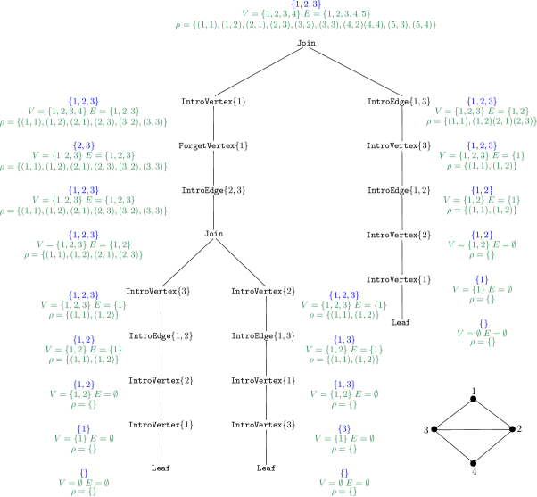
Figure 2: Construction of the graph associated to the $2$-instructive tree decomposition of Fig. 1.

Appendix B Proof of Theorem 4

The proof of Theorem 4 readily follows from results available in the literature. A graph has cliquewidth at most $k$ if and only if it can be defined as the graph associated with a $k$-expression as introduced in [32]. The fact that the set of all $k$-expressions is regular follows directly by the definition of $k$-expression [32, 30]. This shows that cliquewidth is a treelike width measure. In Chapter 12 of [36] it is shown how to define graphs of treewidth at most $k$ using suitable parse trees, and how to associate a graph of treewidth at most $k$ to each such parse tree. The fact that the set of all parse trees corresponding to graphs of treewidth at most $k$ is regular is a direct consequence of the definition. This shows that treewidth is a treelike width measure. Graphs of pathwidth at most $k$ can be obtained by considering a restricted version of the parse-trees considered in [36]. This restriction preserves regularity. Therefore pathwidth is also a treelike width measure. Cutwidth can be shown to be treelike using the notion of slice decompositions considered for instance in [62], while the fact that carving-width is treelike follows from the generalization of slice-decompositions to the context of trees defined in [35]. $\square$

Appendix C Proof of Lemma 7

Next, in Definition 35, we provide a slightly different, but equivalent definition of the notion of tree decomposition of a graph. The only difference is that we replace the condition that requires that for each edge of the graph there is a bag containing the endpoints of that edge, with a choice function $\beta$, which specifies, for each edge $e$, the bag $X_{\beta(e)}$ that contains the endpoints of $e$. We also assume that the tree is rooted, since choosing a root can be done without loss of generality.

Definition 35 (Tree Decomposition).

Let $G$ be a graph. A tree decomposition of $G$ is a triple $(T,X,\beta)$ where $T=(N,F,r)$ is a rooted tree with set of nodes $N$, set of arcs $F$, and root $r$; $\beta:E_{G}\rightarrow N$ is a function mapping each edge $e\in E_{G}$ to some node $p\in N$; and $X=\{X_{u}\}_{u\in N}$ is a collection of subsets of $V_{G}$ satisfying the following properties.

1. For each vertex $x\in V_{G}$, there is some $p\in N$ such that $x\in X_{p}$.

2. For each edge $e\in E_{G}$, $\mathrm{endpts}_{G}(e)\subseteq X_{\beta(e)}$.

3. For each vertex $x\in V_{G}$, the set $\{p\in N\;:\;x\in X_{p}\}$ induces a connected subtree of $T$.

The subsets in $X$ are called bags. The width of $(T,X,\beta)$ is defined as the maximum size of a bag in $X$ minus one: $\mathrm{w}(T,X,\beta)=\max_{p\in N}|X_{p}|-1$. The treewidth of a graph $G$ is the minimum width of a tree decomposition of $G$.

We say that $(T,X,\beta)$ is a nice edge-introducing tree decomposition of $G$ if the function $\beta$ is injective, and additionally, each node $p\in N$ is of one of the following types.

1. $\mathtt{Leaf}$ node: $p$ has no child, and $X_{p}=\emptyset$.

2. $\mathtt{IntroVertex}$ node: $p$ has a unique child $p^{\prime}$ and $X_{p}=X_{p^{\prime}}\cup\{x\}$ for some vertex $x\in V_{G}$. We say that $x$ is introduced at $p$.

3. $\mathtt{ForgetVertex}$ node: $p$ has a unique child $p^{\prime}$ and $X_{p^{\prime}}=X_{p}\cup\{x\}$ for some vertex $x\in V_{G}$. We say that $x$ is forgotten at $p$.

4. $\mathtt{IntroEdge}$ node: $p$ has a unique child $p^{\prime}$, $X_{p}=X_{p^{\prime}}$, and $p=\beta(e)$ for some $e\in E_{G}$. We say that $e$ is introduced at $p$.

5. $\mathtt{Join}$ node: $p$ has two children $p^{\prime}$ and $p^{\prime\prime}$, and $X_{p}=X_{p^{\prime}}=X_{p^{\prime\prime}}$.

We note that our notion of nice, edge-introducing tree decompositions of a graph is essentially identical to the notion of nice tree decompositions with introduce-edge nodes used in the literature (see [33], pages 161 and 168), except that we do not require the root bag to be empty. The fact that arbitrary tree decompositions can be efficiently transformed into nice, edge-introducing tree decompositions is an easy exercise (see for instance Lemma 7.4 of [33]).

Observation 36.

Let $G$ be a graph, and $(T,X,\beta)$ be a tree decomposition $G$ of width at most $k$, where $T=(N,F,r)$. Then, one can construct in time $O(k^{2}\cdot\max\{|V_{G}|,|N|\}+|E_{G}|)$ a nice, edge-introducing tree decomposition $(T^{\prime},X^{\prime},\beta^{\prime})$ of $G$ of width at most $k$ that has $O(k\cdot|V_{G}|+|E_{G}|)$ nodes.

Now, we are in a position to prove that a graph $G$ is isomorphic to the graph $\mathcal{G}(\tau)$ associated with some $k$-instructive tree decomposition $\tau$ if and only if $G$ has treewidth at most $k$.

First, let $\tau$ be a $k$-instructive tree decomposition, and $\mathcal{G}(\tau)$ be its associated graph. Then this graph can be obtained from smaller graphs of size at most $k+1$ by successively identifying sub-graphs of size at most $k+1$. This implies that $\mathcal{G}(\tau)$ is a subgraph of a $k$-tree, and therefore that $\mathcal{G}(\tau)$ has treewidth at most $k$.

Claim 37.

Let $\tau$ be a $k$-instructive tree decomposition. Then, the graph $\mathcal{G}(\tau)$ has a nice edge-introducing tree decomposition $(T,X,\beta)$ of width at most $k$ where the bag associated with the root node $r$ is the set $X_{r}=\theta[\tau](B(\tau))$.

Proof.

The proof is by induction on the height $h$ of $\tau$. In the base case, $h=0$. In this case, $\tau=\mathtt{Leaf}$. Therefore, since $\mathcal{G}(\tau)$ is the empty graph, the claim is vacuously satisfied. Now, suppose the claim is valid for every $k$-instructive tree decomposition $\tau$ of height at most $h$, and let $\tau$ be a $k$-instructive tree decomposition of height $h+1$. There are four cases to be analyzed.

• Let $\sigma$ be a $k$-instructive tree decompositions of height at most $h$ and let $(T,X,\beta)$ be a nice edge-introducing tree decompositions with roots $r$ root-bag $X_{r}$ satisfying the conditions of the claim. In this case we create a new root node $r^{\prime}$ with root bag $X_{r^{\prime}}$, and set $r$ as the child of $r^{\prime}$.

  1. If $\tau=\mathtt{IntroVertex}\{u\}(\sigma)$, we let $X_{r^{\prime}}=X_{r}\cup\{\theta[\tau](u)\}$.

  2. If $\tau=\mathtt{ForgetVertex}\{u\}(\sigma)$, we let $X_{r^{\prime}}=X_{r}\backslash\{\theta[\tau](u)\}$.

  3. If $\tau=\mathtt{IntroEdge}\{u,v\}(\sigma)$, we let $X_{r^{\prime}}=X_{r}$.

• Let $\sigma_{1}$ and $\sigma_{2}$ be $k$-instructive tree decompositions of height at most $h$ and let $(T_{1},X_{1},\beta_{1})$ and $(T_{2},X_{2},\beta_{2})$ be their respective nice edge-introducing tree decompositions with roots $r_{1}$ and $r_{2}$ and root-bags $X_{r_{1}}$ and $X_{r_{2}}$ satisfying the conditions of the claim.

  1. Let $\tau=\mathtt{Join}(\sigma_{1},\sigma_{2})$. In this case, we create a new root bag $r$, labeled with the bag $X_{r}=X_{r_{1}}$ and set $r_{1}$ and $r_{2}$ as the children of $r$. Additionally, in the new tree decomposition, for each node $p$ of $T_{2}$, the bag $X_{p}$ is replaced by the bag

     $$X^{\prime}_{p}=\{\theta[\tau_{1}](u)\;:\;u\in B(\tau),\;\theta[\tau_{2}](u)\in X_{p}\}\cup\{x+a\;:\;x\in X_{p}\backslash\theta[\tau](B(\tau))\}.$$

     where $a=\max V_{\mathcal{G}(\tau)}$. Note that this renumbering is necessary because the vertices of $\mathcal{G}(\tau_{2})$ are renumbered by the join operation $(\mathcal{G}(\tau_{1}),\theta[\tau])\oplus(\mathcal{G}(\tau_{2}),\theta[\tau_{2}])$.

It is straightforward to check that in each of the four cases, the obtained tree decomposition satisfies the conditions of the claim. ∎

Let $G$ be a graph and $\alpha:V_{G}\rightarrow[k+1]$ be a proper $(k+1)$-coloring of $G$. More specifically, for each edge $e\in E_{G}$ the endpoints of $e$ are colored differently by $\alpha$. We say that $\alpha$ is bag-injective with respect to a nice, edge introducing tree decomposition $(T,X,\beta)$ of $G$ if for each bag $X_{p}\in X$, the restriction $\alpha|_{X_{p}}$ is injective.

Observation 38.

Let $G$ be a graph and $(T,X,\beta)$ be a tree decomposition of width $k$ of $G$, where $T=(N,F,r)$. Then, one can construct in time $O(k\cdot|N|)$ a proper $(k+1)$-coloring $\alpha$ of $G$ that is bag-injective for $(T,X,\beta)$.

Proof.

We will construct a coloring $\alpha:V_{G}\rightarrow[k+1]$ of $G$ that is bag-injective for $(T,X,\beta)$ by traversing the bags in $X$ from the root towards the leaves. We start by choosing an arbitrary injective coloring of the vertices in the root bag $X_{r}$. Since $X_{r}$ has at most $k+1$ vertices, such an injective coloring with at most $(k+1)$ colors exists. Now assume that the vertices of a given bag $X_{p}$ have been injectively colored with at most $k+1$ colors, and let $p^{\prime}$ be a child of $p$. Then we have three possibilities: (i) $X_{p^{\prime}}=X_{p}$; (ii) $X_{p^{\prime}}=X_{p}\backslash\{x\}$, for some vertex $x$; (iii) $X_{p^{\prime}}=X_{p}\cup\{x\}$ for some vertex $x$. In the first two cases, an injective coloring of the vertices in $X_{p^{\prime}}$ has already been chosen. In the last case, we just choose some arbitrary color for $x$ in the set $[k+1]\backslash\alpha(X_{p})$. We proceed in this way until all bags have been visited. Since each vertex occurs in some bag, each vertex has received some color from the set $[k+1]$. Since the endpoints of each edge $e$ are contained in some bag, and since by construction, the coloring in each bag is injective, we have that the endpoints of $e$ receive distinct colors. Therefore, $\alpha$ is a proper $(k+1)$-coloring of $G$. ∎

Now, let $G$ be a graph of treewidth at most $k$. Let $(T,X,\beta)$ be a nice, edge-introducing tree decomposition of $G$ of width at most $k$. Let $\alpha:V_{G}\rightarrow[k+1]$ be a proper $(k+1)$-coloring of $G$ that is bag-injective for $(T,X,\beta)$. By Observation 38 such a coloring exists and can be constructed in time $O(k\cdot|N|)$ where $N$ is the set of nodes of $T$. Then, a $k$-instructive tree decomposition $\tau$ of $G$ can be constructed as follows. We let $\tau$ have the same structure as $T$, except that instead being labeled with bags, the nodes are now labeled with instructions from the alphabet $\Sigma_{k}$. More specifically, each leaf node is labeled with the instruction $\mathtt{Leaf}$. Now, let $p$ be a node of $T$. If a vertex $x$ is introduced at $p$, then we label the node $p$ of $\tau$ with the instruction $\mathtt{IntroVertex}\{\alpha(x)\}$. If an edge $\{x,y\}$ is introduced at $p$, then the node $p$ of $\tau$ is labeled with the instruction $\mathtt{IntroEdge}\{\alpha(x),\alpha(y)\}$. If a vertex $x$ is forgotten at $p$, then the node $p$ of $\tau$ is labeled with the instruction $\mathtt{ForgetVertex}\{\alpha(x)\}$. Finally, $p$ is a join node, then the node $p$ of $\tau$ is labeled with the instruction $\mathtt{Join}$. This concludes the proof of Lemma 7. $\square$

Appendix D Proof of Lemma 19

In this section, we prove Lemma 19 by induction on the height of a $k$-instructive tree decomposition $\tau$. Although the proof is straightforward, it serves as an illustration of how the objects $B(\tau)$, $\mathcal{G}(\tau)$, $\theta[\tau]$ and $\Gamma[{\mathsf{D},k}](\tau)$ interact in an inductive proof of correctness of a DP-core $\mathsf{D}$. In particular, the structure of this proof can be adapted to provide inductive proofs for the correctness of DP-cores deciding other graph properties.

Base Case: In the base case, the height of $\tau$ is $0$, and therefore $\tau=\mathtt{Leaf}$. By Definition 9 and Definition 18.1, $\Gamma[{\texttt{\mbox{$\mathtt{C}$-$\mathtt{VertexCover}$}}_{r},k}](\tau)=\texttt{\mbox{$\mathtt{C}$-$\mathtt{VertexCover}$}}_{r}[k].\mathtt{LeafSet}=\{(\emptyset,0)\}$. Since $\mathcal{G}(\tau)=(\emptyset,\emptyset,\emptyset)$, we have that $\emptyset$ is the only vertex cover of $\mathcal{G}(\tau)$, and since this vertex cover has size $0$, $\mathsf{w}=(\emptyset,0)$ is the only local witness with $\texttt{P-VertexCover}_{r}(\tau,\mathsf{w})=1$. Therefore, the lemma holds in the base case.

Inductive Step: Now, assume that the lemma holds for every $k$-instructive tree decomposition of height at most $h$. Let $\tau$ be a $k$-instructive tree decomposition of height $h+1$, and $\mathsf{w}=(R,s)$ be a local witness in $\texttt{\mbox{$\mathtt{C}$-$\mathtt{VertexCover}$}}_{r}[k].\mathcal{W}$. There are four cases to be considered.

1. Let $\tau=\mathtt{IntroVertex}\{u\}(\sigma)$. Suppose $\mathsf{w}\in\Gamma[{\texttt{\mbox{$\mathtt{C}$-$\mathtt{VertexCover}$}}_{r},k}](\tau)$. By Definition 9 and Definition 18.2, we have that $\mathsf{w}$ also belongs to $\Gamma[{\texttt{\mbox{$\mathtt{C}$-$\mathtt{VertexCover}$}}_{r},k}](\sigma)$. By the induction hypothesis, $\texttt{P-VertexCover}_{r}[k](\sigma,\mathsf{w})=1$. Then, $s\leq r$, and $s$ is the minimum size of a vertex cover $X$ in $\mathcal{G}(\sigma)$ with $\theta[\sigma](R)=X\cap Im(\theta[\sigma](B(\sigma)))$. This implies that $X$ is also a vertex cover in $\mathcal{G}(\tau)$ with $\theta[\tau](R)=X\cap Im(\theta[\tau](B(\tau)))$. Therefore, $\texttt{P-VertexCover}_{r}[k](\tau,\mathsf{w})=1$.

   For the converse, let $\texttt{P-VertexCover}_{r}[k](\tau,\mathsf{w})=1$. Then, there is a vertex cover $X$ of $\mathcal{G}(\tau)$ of size $s$ where $\theta[\tau](R)=X\cap Im(\theta[\tau](B(\tau)))$ and $s$ is the minimum size of such vertex cover. Since $E_{\mathcal{G}(\tau)}=E_{\mathcal{G}(\sigma)}$, the vertex cover $X$ is a vertex cover of $\mathcal{G}(\sigma)$ such that $\theta[\sigma](R)=X\cap Im(\theta[\sigma](B(\sigma)))$. Therefore, $\texttt{P-VertexCover}_{r}[k](\sigma,\mathsf{w})=1$. By the induction hypothesis, $\mathsf{w}\in\Gamma[{\texttt{\mbox{$\mathtt{C}$-$\mathtt{VertexCover}$}}_{r},k}](\sigma)$. By Definition 18.2, we have that $\texttt{\mbox{$\mathtt{C}$-$\mathtt{VertexCover}$}}_{r}[k].\mathtt{IntroVertex}\{u\}(\mathsf{w})=\{\mathsf{w}\}$. Therefore, $\mathsf{w}\in\Gamma[{\texttt{\mbox{$\mathtt{C}$-$\mathtt{VertexCover}$}}_{r},k}](\tau)$.

2. Let $\tau=\mathtt{ForgetVertex}\{u\}(\sigma)$. Suppose $\mathsf{w}\in\Gamma[{\texttt{\mbox{$\mathtt{C}$-$\mathtt{VertexCover}$}}_{r},k}](\tau)$. By Definition 18.3, there exists $\mathsf{w}^{\prime}=(R^{\prime},s^{\prime})\in\Gamma[{\texttt{\mbox{$\mathtt{C}$-$\mathtt{VertexCover}$}}_{r},k}](\sigma)$ such that
   $\texttt{\mbox{$\mathtt{C}$-$\mathtt{VertexCover}$}}_{r}[k].\mathtt{ForgetVertex}\{u\}(\mathsf{w}^{\prime})=\{\mathsf{w}\}$. Note that $R^{\prime}\setminus\{u\}=R$ and $s^{\prime}=s$. By the induction hypothesis, $\texttt{P-VertexCover}_{r}[k](\sigma,\mathsf{w}^{\prime})=1$, and therefore, there exists a vertex cover $X$ of minimum size $s^{\prime}$ in $\mathcal{G}(\sigma)$ where $\theta[\sigma](R^{\prime})=X\cap Im(\theta[\sigma](B(\sigma)))$. Since $\mathcal{G}(\sigma)=\mathcal{G}(\tau)$, the set $X$ is a vertex cover of $\mathcal{G}(\tau)$. We can infer the following by the fact that $B(\tau)=B(\sigma)\setminus\{u\}$, $R=R^{\prime}\setminus\{u\}$, and $\theta[\tau]=\theta[\sigma]|_{B(\tau)}$:

   $$\theta[\tau](R)=X\cap Im(\theta[\tau](B(\tau)))$$ (4)

   Since $X$ is a vertex cover of minimum size in $\mathcal{G}(\sigma)$ such that $\theta[\sigma](R^{\prime})=X\cap Im(\theta[\sigma](B(\sigma)))$ and since $\mathcal{G}(\tau)=\mathcal{G}(\sigma)$, we have that $X$ is also a vertex cover of minimum size in $\mathcal{G}(\tau)$ that satisfies Equation 4. Consequently, $\texttt{P-VertexCover}_{r}[k](\tau,\mathsf{w})=1$.

   For the converse, suppose $\texttt{P-VertexCover}_{r}[k](\tau,\mathsf{w})=1$. Then, there is a vertex cover $X$ of minimum size such that $\theta[\tau](R)=X\cap Im(\theta[\tau](B(\tau)))$ and $|X|=s\leq r$. Since $\mathcal{G}(\tau)=\mathcal{G}(\sigma)$, the set $X$ is a vertex cover of $\mathcal{G}(\sigma)$. There are two cases to be considered:

   1. $\theta[\sigma](u)\in X$. In this case, let $\mathsf{w}^{\prime}=(R^{\prime},s)$ where $R^{\prime}=R\cup\{u\}$.

   2. $\theta[\sigma](u)\notin X$. In this case, let $\mathsf{w}^{\prime}=(R^{\prime},s)$ where $R^{\prime}=R$.

   In both cases we will show that $\mathsf{w}^{\prime}\in\Gamma[{\texttt{\mbox{$\mathtt{C}$-$\mathtt{VertexCover}$}}_{r}}]{k}(\sigma)$. Recall that $B(\tau)=B(\sigma)\setminus\{u\}$ and $\theta[\tau]=\theta[\sigma]|_{B(\tau)}$, and therefore we have that

   $$\theta[\sigma](R^{\prime})=X\cap Im(\theta[\sigma](B(\sigma))).$$ (5)

   Equation 5 holds for the two cases and $X$ is a vertex cover of minimum size satisfying Equation 5. Then, $\texttt{P-VertexCover}_{r}[k](\sigma,\mathsf{w}^{\prime})=1$, and by the induction hypothesis, $\mathsf{w}^{\prime}\in\Gamma[{\texttt{\mbox{$\mathtt{C}$-$\mathtt{VertexCover}$}}_{r},k}](\sigma)$. By Definition 18.3, $\texttt{\mbox{$\mathtt{C}$-$\mathtt{VertexCover}$}}_{r}[k].\mathtt{ForgetVertex}\{u\}(\mathsf{w}^{\prime})=\{(R^{\prime}\setminus\{u\},s)\}$ and we have that $(R^{\prime}\setminus\{u\},s)=\mathsf{w}$, and therefore, $\mathsf{w}\in\Gamma[{\texttt{\mbox{$\mathtt{C}$-$\mathtt{VertexCover}$}}_{r},k}](\tau)$.

3. Let $\tau=\mathtt{IntroEdge}\{u,v\}(\sigma)$. Suppose $\mathsf{w}\in\Gamma[{\texttt{\mbox{$\mathtt{C}$-$\mathtt{VertexCover}$}}_{r},k}](\sigma)$. By Definition 18.4, there exists $\mathsf{w}^{\prime}=(R^{\prime},s^{\prime})\in\Gamma[{\texttt{\mbox{$\mathtt{C}$-$\mathtt{VertexCover}$}}_{r},k}](\sigma)$ where
   $\texttt{\mbox{$\mathtt{C}$-$\mathtt{VertexCover}$}}_{r}[k].\mathtt{IntroEdge}\{u,v\}(\mathsf{w}^{\prime})=\{\mathsf{w}\}$ and either $(R,s)=(R^{\prime},s^{\prime})$ or $(R,s)=(R^{\prime}\cup\{x\},s^{\prime}+1)$ where $x\in\{u,v\}$. By the induction hypothesis, $\texttt{P-VertexCover}_{r}[k](\sigma,\mathsf{w}^{\prime})=1$, and therefore, there is a vertex cover $X$ of minimum size where $\theta[\sigma](R^{\prime})=X\cap Im(\theta[\sigma](B(\sigma)))$. We consider two cases and define $X^{\prime}$ with regards to these cases.

   1. $R=R^{\prime}\cup\{x\}$ where $x\in\{u,v\}$. In this case let $X^{\prime}=X\cup\{\theta[\tau](x)\}$.

   2. $R=R^{\prime}$. In this case let $X^{\prime}=X$.

   Note that $E_{\mathcal{G}(\tau)}=E_{\mathcal{G}(\sigma)}\cup\{e\}$ where $(e,\theta[\tau](u)),(e,\theta[\tau](v))\in\rho_{\mathcal{G}(\tau)}$ so that $X^{\prime}$ is a vertex cover of $\mathcal{G}(\tau)$. Recall that $B(\tau)=B(\sigma)$ and $\theta[\tau]=\theta[\sigma]$. We can infer the following equation by the fact that we have mentioned.

   $$\theta[\tau](R)=X^{\prime}\cap Im(\theta[\tau](B(\tau)))$$ (6)

   If we show $X^{\prime}$ is a vertex cover of minimum size satisfying 6, then we have proved the statement. Next, we will prove the vertex cover $X^{\prime}$ is minimum size. Suppose $X^{\prime}=X$ (the second case), then obviously $X^{\prime}$ is minimum size. Otherwise, suppose $X^{\prime}=X\cup\{\theta[\tau](x)\}$ (the first case) and suppose $X^{\prime}$ is not a vertex cover of minimum size and there is a vertex cover $|X^{\prime\prime}|<|X^{\prime}|$ where $\theta[\tau](R)=X^{\prime\prime}\cap Im(\theta[\tau](B(\tau)))$. Therefore, we have $\theta[\tau](R^{\prime})=(X^{\prime\prime}\setminus\{\theta[\tau](x)\})\cap Im(\theta[\tau](B(\sigma)))$ and we know $|X^{\prime\prime}\setminus\{\theta[\tau](x)\}|<|X|$, and therefore, this contradicts the assumption that $X$ is the minimum size vertex cover which satisfies the second condition of the definition of $\texttt{P-VertexCover}_{r}$.

   For the converse, suppose $\texttt{P-VertexCover}_{r}[k](\tau,\mathsf{w})=1$. Then, there exists a vertex cover $X$ where $\theta[\tau](R)=X\cap Im(\theta[\tau](B(\tau)))$ where $X$ is the minimum size of such vertex cover. In the following let $e$ be the edge that $\theta[\tau](u)$ and $\theta[\tau](v)$ are the endpoints of it.

   1. $X\setminus\{\theta[\tau](x)\}$ where $x\in\{u,v\}$ is a vertex cover of $\mathcal{G}(\tau)\setminus\{e\}$. In this case let $\mathsf{w}^{\prime}=(R^{\prime},s^{\prime})$ where $R^{\prime}=R\setminus\{u,v\}$ and $s^{\prime}=s-1$, and let $X^{\prime}=X\setminus\{\theta[\tau](x)\}$.

   2. $X\setminus\{\theta[\tau](x)\}$ where $x\in\{u,v\}$ is not a vertex cover of $\mathcal{G}(\tau)\setminus\{e\}$. In this case, we set $\mathsf{w}^{\prime}=(R^{\prime},s^{\prime})$ where $R^{\prime}=R$ and $s^{\prime}=s$, and let $X^{\prime}=X$.

   In both cases, we show that $\texttt{P-VertexCover}_{r}[k](\sigma,\mathsf{w}^{\prime})=1$. The condition $s^{\prime}\leq r$, is satisfied. Since $\mathcal{G}(\tau)=\mathcal{G}(\sigma)\setminus\{e\}$, $X^{\prime}$ in both cases is a vertex cover of $\mathcal{G}(\sigma)$. We have $B(\tau)=B(\sigma)$ and $\theta[\tau]=\theta[\sigma]$, and therefore in the both cases the following equation is satisfied.

   $$\theta[\sigma](R^{\prime})=X^{\prime}\cap Im(\theta[\sigma](B(\sigma)))$$ (7)

   Now it remains that we show $X^{\prime}$ is the minimum size vertex cover where satisfying Equation 7. If $X^{\prime}=X$ and since $X$ is minimum size, $X^{\prime}$ is minimum size. If $X^{\prime}=X\setminus\{\theta[\tau](x)\}$ and suppose $X^{\prime}$ is not minimum size, therefore, there exists a vertex cover $X^{\prime\prime}$ where $\theta[\sigma](R^{\prime})=X^{\prime\prime}\cap Im(\theta[\sigma](B(\sigma)))$ such that $|X^{\prime\prime}|<|X^{\prime}|$, and consequently, we have $|X^{\prime\prime}\cup\{\theta[\tau](x)\}|<|X|$ and $\theta[\tau](R)=(X^{\prime\prime}\cup\{\theta[\tau](x)\})\cap Im(\theta[\tau](B(\tau)))$ and this contradicts the assumption that $X$ is minimum size. Therefore, $X^{\prime}$ is minimum size, and consequently, $\texttt{P-VertexCover}_{r}[k](\sigma,\mathsf{w}^{\prime})=1$. By the induction hypothesis, $\mathsf{w}^{\prime}\in\Gamma[{\texttt{\mbox{$\mathtt{C}$-$\mathtt{VertexCover}$}}_{r},k}](\sigma)$. By Definition 18.4, $\texttt{\mbox{$\mathtt{C}$-$\mathtt{VertexCover}$}}_{r}[k](\mathsf{w}^{\prime})=\{\mathsf{w}\}$, and therefore, $\mathsf{w}\in\Gamma[{\texttt{\mbox{$\mathtt{C}$-$\mathtt{VertexCover}$}}_{r}}]{k}(\tau)$.

4. Let $\tau=\mathtt{Join}(\sigma_{1},\sigma_{2})$. Suppose $\mathsf{w}\in\Gamma[{\texttt{\mbox{$\mathtt{C}$-$\mathtt{VertexCover}$}}_{r},k}](\tau)$. Let $\mathsf{w}_{1}=(R_{1},s_{1})\in\Gamma[{\texttt{\mbox{$\mathtt{C}$-$\mathtt{VertexCover}$}}_{r},k}](\sigma_{1})$ and $\mathsf{w}_{2}=(R_{2},s_{2})\in\Gamma[{\texttt{\mbox{$\mathtt{C}$-$\mathtt{VertexCover}$}}_{r},k}](\sigma_{2})$ be two local witnesses such that $\texttt{\mbox{$\mathtt{C}$-$\mathtt{VertexCover}$}}_{r}[k].\mathtt{Join}(\mathsf{w}_{1},\mathsf{w}_{2})=\{\mathsf{w}\}$, and by Definition 18.5, $R=R_{1}\cup R_{2}$ and $s=s_{1}+s_{2}-|R_{1}\cap R_{2}|$ where $s\leq r$. By the induction hypothesis, since $\mathsf{w}_{i}\in\Gamma[{\texttt{\mbox{$\mathtt{C}$-$\mathtt{VertexCover}$}}_{r},k}](\sigma_{i})$, we have $\texttt{P-VertexCover}_{r}[k](\sigma_{i},\mathsf{w}_{i})=1$ for $i\in\{1,2\}$. Therefore, there exists a vertex cover $X_{i}$ of minimum size of $\mathcal{G}(\sigma_{i})$ where $\theta[\sigma_{i}](R_{i})=X_{i}\cap Im(\theta[\sigma_{i}](B(\sigma_{i})))$. Let $X=X_{1}\cup\{v+a\;:\;v\in X_{2}\setminus\theta[\sigma_{2}](B(\sigma_{2}))\}$ where $a=\max\{v:v\in V_{\mathcal{G}(\sigma_{1})}\}$. Let $\zeta:V_{\mathcal{G}(\sigma_{2})}\to V_{\mathcal{G}(\tau)}$ be the map between corresponding labels of vertices in $\mathcal{G}(\sigma_{2})$ and $\mathcal{G}(\tau)$. More specifically, we let $a=\max\{v\;:\;v\in V_{G_{1}}\}$, and set for each $x\in V_{\mathcal{G}(\sigma_{2})}$

   $$\zeta(x)=\begin{cases}\theta[\tau]\big{(}\theta[\sigma_{2}]^{-1}(x)\big{)}&\mbox{ if }x\in Range(\theta[\sigma_{2}])\\ x+a&\mbox{ if }x\notin Range(\theta[\sigma_{2}])\end{cases}$$

   By the fact that $B(\tau)=B(\sigma_{2})$ and that $R_{2}\subseteq B(\sigma_{2})$, we can infer that $\zeta(\theta[\sigma_{2}](R_{2}))=\theta[\tau](R_{2})$, $\zeta(Im(\theta[\sigma_{2}](B(\sigma_{2}))))=Im(\theta[\tau](B(\tau)))$, $\zeta(X_{2})=(X\setminus X_{1})\cup\theta[\tau](R_{2})$, and $X=X_{1}\cup\zeta(X_{2})$. Therefore, we have the following.

   $$\begin{array}[]{cl}&\zeta(\theta[\sigma_{2}](R_{2}))=\zeta(X_{2})\cap\zeta(Im(\theta[\sigma_{2}](B(\sigma_{2}))))\\ \implies&\theta[\tau](R_{2})=X^{\prime}_{2}\cap Im(\theta[\tau](B(\tau)))\\ \end{array}$$ (8)

   where $X^{\prime}_{2}=\zeta(X_{2})$. The set $X$ is a vertex cover of $\mathcal{G}(\tau)$ since each edge is either in $\mathcal{G}(\sigma_{1})$ or $\mathcal{G}(\sigma_{2})$. If an edge is in $\mathcal{G}(\sigma_{1})$, then at least one of the endpoints is in $X_{1}$ and if an edge is in $\mathcal{G}(\sigma_{2})$, then at least one endpoints is in $X^{\prime}_{2}$. By the fact $\theta[\sigma_{1}](R_{1})=X_{1}\cap Im(\theta[\sigma_{1}](B(\sigma_{1})))$, $B(\tau)=B(\sigma_{1})=B(\sigma_{2})$, $\theta[\tau]=\theta[\sigma_{1}]$, and Equation 8, we can infer the following.

   $$\begin{array}[]{l}\theta[\tau](R_{1})\cup\theta[\tau](R_{2})=\big{(}X_{1}\cap Im(\theta[\tau](B(\tau)))\big{)}\cup\big{(}X^{\prime}_{2}\cap Im(\theta[\tau](B(\tau)))\big{)}\\ \implies\theta[\tau](R_{1})\cup\theta[\tau](R_{2})=(X_{1}\cup X^{\prime}_{2})\cap Im(\theta[\tau](B(\tau)))\\ \implies\theta[\tau](R)=X\cap Im(\theta[\tau](B(\tau)))\end{array}$$ (9)

   The vertex cover $X$ satisfies Equation 9 and if we show that $s$ is the minimum size of such vertex cover satisfying Equation 9, then we have proved the statement. Suppose $X$ is not a vertex cover of minimum size and there exists a vertex cover $\mathcal{M}$ such that $|\mathcal{M}|<|X|$ where $\theta[\tau](R)=\mathcal{M}\cap Im(\theta[\tau](B(\tau)))$. Let $\mathcal{M}_{1}=\mathcal{M}\cap V_{\mathcal{G}(\sigma_{1})}$ and $\mathcal{M}_{2}=\zeta^{-1}(\mathcal{M}\cap\zeta(V_{\mathcal{G}(\sigma_{2})}))$ be vertex covers of $\mathcal{G}(\sigma_{1})$ and $\mathcal{G}(\sigma_{2})$ satisfying the following equation.

   $$\theta[\sigma_{i}](R_{i})=\mathcal{M}_{i}\cap Im(\theta[\sigma_{i}](B(\sigma_{i})))$$ (10)

   for $i\in\{1,2\}$. We have $\mathcal{M}_{1}\cup\zeta(\mathcal{M}_{2})=\mathcal{M}$, and consequently, the following equation holds.

   $$|\mathcal{M}|=|\mathcal{M}_{1}\cup\zeta(\mathcal{M}_{2})|=|\mathcal{M}_{1}|+|\zeta(\mathcal{M}_{2})|-|\mathcal{M}_{1}\cap\zeta(\mathcal{M}_{2})|$$ (11)

   Also we have the following,

   $$|X|=|X_{1}\cup\zeta(X_{2})|=|X_{1}|+|\zeta(X_{2})|-|X_{1}\cap\zeta(X_{2})|$$ (12)

   We know $X_{i}$ is a vertex cover of minimum size of $\mathcal{G}(\sigma_{i})$ satisfying Equation 10, and therefore, $|X_{i}|\leq|\mathcal{M}_{i}|$, and also by $\theta[\tau](R_{1}\cap R_{2})=\mathcal{M}_{1}\cap\zeta(\mathcal{M}_{2})=X_{1}\cap\zeta(X_{2})$, Equation 11, and Equation 12 we can infer $|X|\leq|\mathcal{M}|$. This contradicts the assumption that $|\mathcal{M}|<|X|$, and therefore, $X$ is minimum size. As a consequence, $\texttt{P-VertexCover}_{r}[k](\tau,\mathsf{w})=1$.

   For the converse, suppose $\texttt{P-VertexCover}_{r}[k](\tau,\mathsf{w})=1$. There is a vertex cover $X$ where satisfies the second Condition of the definition of $\texttt{P-VertexCover}_{r}$. Let $R_{1}=\theta[\tau]^{-1}(X\cap V_{\mathcal{G}(\sigma_{1})}\cap\theta[\sigma_{1}](B(\sigma_{1})))$, $s_{1}=|X\cap V_{\mathcal{G}(\sigma_{1})}|$, and $X_{1}=X\cap V_{\mathcal{G}(\sigma_{1})}$. Also, let $R_{2}=\theta[\tau]^{-1}\Big{(}X\cap\zeta(V_{\mathcal{G}(\sigma_{2})})\cap\zeta(\theta[\sigma_{2}](B(\sigma_{2})))\Big{)}$, $s_{2}=|X\cap\zeta(V_{\mathcal{G}(\sigma_{2})})|$, and $X_{2}=\zeta^{-1}(X\cap\zeta(V_{\mathcal{G}(\sigma_{2})}))$. The following equation holds for the defined sets.

   $$\theta[\sigma_{i}](R_{i})=X_{i}\cap Im(\theta[\sigma_{i}](B(\sigma_{i})))$$ (13)

   Let $\mathsf{w}_{i}=(R_{i},s_{i})$ and we will show that $\texttt{P-VertexCover}_{r}[k](\sigma_{i},\mathsf{w}_{i})=1$ for $i\in\{1,2\}$. To prove it, we need to show $X_{i}$ is a vertex cover of minimum size satisfying Equation 13. Suppose it is not minimum, and there is a vertex cover $|X^{\prime}_{1}|<|X_{1}|$ (same argument for $X_{2}$) that satisfies $\theta[\sigma_{1}](R_{1})=X_{1}\cap Im(\theta[\sigma_{1}](B(\sigma_{1})))$. The set $X^{\prime}=X^{\prime}_{1}\cup\zeta(X_{2})$ is also a vertex cover of $\mathcal{G}(\tau)$ where $\theta[\tau](R)=X^{\prime}\cap Im(\theta[\tau](B(\tau)))$ and $|X^{\prime}|<|X|$. This contradicts the assumption that $X$ is a vertex cover of minimum size.

   We have proved $\texttt{P-VertexCover}_{r}[k](\sigma_{i},\mathsf{w}_{i})=1$, and therefore, by the induction hypothesis, $\mathsf{w}_{i}\in\Gamma[{\texttt{\mbox{$\mathtt{C}$-$\mathtt{VertexCover}$}}_{r},k}](\sigma_{i})$ for $i\in\{1,2\}$. By Definition 18.5, we have that $\texttt{\mbox{$\mathtt{C}$-$\mathtt{VertexCover}$}}_{r}[k].\mathtt{Join}(\mathsf{w}_{1},\mathsf{w}_{2})=\{\mathsf{w}\}$, and therefore, $\mathsf{w}\in\Gamma[{\texttt{\mbox{$\mathtt{C}$-$\mathtt{VertexCover}$}}_{r},k}](\tau)$. $\square$

Appendix E Proof of Theorem 34

In this section, we prove Theorem 34. More specifically, for each graph property $\mathbb{P}$ listed in Theorem 34, we provide an upper bound for the bit-length $\beta_{\mathsf{D}}(k)$ of a suitable $\mathsf{ITD}$-coherent DP-core $\mathsf{D}$ with $\mathbb{G}[\mathsf{D},\mathsf{ITD}]=\mathbb{P}$. The multiplicity of such a DP-core $\mathsf{D}$ is trivially upper bounded by $2^{O(\beta_{\mathsf{D}}(k))}$, the state complexity of $\mathsf{D}$ is trivially upper bounded by $2^{O(\beta_{\mathsf{D}}(k))}$, and the deterministic state complexity of $\mathsf{D}$ is trivially upper bounded by $2^{2^{O(\beta_{\mathsf{D}}(k))}}$. In some cases, we show that that these two last upper bounds can be improved using additional arguments.

The process of specifying a coherent DP-core $\mathsf{D}$ deciding a given graph property $\mathbb{P}$ can be split into four main steps, which should hold for each $k\in\mathbb{N}$.

1. The specification of a suitable set $\mathsf{D}[k].\mathcal{W}$ of local witnesses, and of a Boolean function $\mathsf{D}[k].\mathtt{Final}$ determining which are the final local witnesses in $\mathsf{D}[k].\mathcal{W}$.

2. The specification of a predicate $\texttt{P}[k]\subseteq\mathsf{ITD}_{k}\times\mathsf{D}[k].\mathcal{W}$ such that for each $\tau\in\mathsf{ITD}_{k}$, and each final local witness $\mathsf{w}$, $(\tau,\mathsf{w})\in\texttt{P}[k]$ if and only if the graph $\mathcal{G}(\tau)$ belongs to $\mathbb{P}$.

3. The specification of the functions belonging to $\mathsf{D}[k]$.

4. An inductive proof that for each pair $(\tau,\mathsf{w})\in\mathsf{ITD}_{k}\times\mathsf{D}[k].\mathcal{W}$, $(\tau,\mathsf{w})\in\Gamma[{\mathsf{D},k}](\tau)$ if and only if $(\tau,\mathsf{w})\in\texttt{P}[k]$. This last step together with Step 2 guarantees that the DP-core is coherent and that $\mathbb{G}[\mathsf{D}[k]]=\mathbb{P}$.

The process described above was exemplified in full detail with respect to the DP-core $\texttt{\mbox{$\mathtt{C}$-$\mathtt{VertexCover}$}}_{r}$ defined in Section 5.3. In this case, Steps 1, 2 and 3 were carried out in Section 5.3, and Step 4 was carried out in Appendix D. In this section, we are only interested in providing an upper bound on the bitlength of the DP-cores listed in Theorem 34. Therefore, we will only carry out in details Steps 1 and 2, which are the ones that require ingenuity. Once this is done, it is straightforward to specify the functions of $\mathsf{D}[k]$ in such a way that the requirement

$$(\tau,\mathsf{w})\in\Gamma[{\mathsf{D},k}](\tau)\Leftrightarrow(\tau,\mathsf{w})\in\texttt{P}[k]$$

is satisfied by construction. A full inductive proof of correctness of the specification, as exemplified in Section D is also straightforward.

Our choices of local witnesses is based on simplicity, instead of efficiency, and our goal primarily to justify the asymptotic upper bounds listed in Theorem 34.

E.1 C-Simple

The graph property of the DP-core C-Simple is the set Simple of all simple graphs. For each $k\in\mathbb{N}$, a local witness for $\texttt{C-Simple}[k]$ is a subset $\mathsf{w}\subseteq\binom{[k+1]}{2}$. All local witnesses are final. The transitions of $\texttt{C-Simple}[k]$ are defined in such a way that for each $k$-instructive tree decomposition $\tau$ and each local witness $\mathsf{w}$, $\mathsf{w}\in\Gamma[{\texttt{C-Simple},k}](\tau)$ if and only if the following predicate is satisfied:

• $\texttt{P-Simple}[k](\tau,\mathsf{w})\equiv$ $\mathcal{G}(\tau)$ is a simple graph, and for each two distinct elements $u$ and $v$ in $[k+1]$, $\{u,v\}\in\mathsf{w}$ if and only if there is a unique edge $e\in E_{\mathcal{G}(\tau)}$ such that $\mathrm{endpts}_{\mathcal{G}(\tau)}(e)=\{\theta[\tau](u),\theta[\tau](v)\}$.

Each local witness $\mathsf{w}$ may be represented as a Boolean vector in $\{0,1\}^{\binom{k+1}{2}}$ which has one coordinate for each pair $\{u,v\}\in\mathsf{w}$. The DP-core $\texttt{C-Simple}[k]$ can be defined in such a way that it is deterministic, in the sense that the set obtained from each local witness $\mathsf{w}$ upon the application of each transition is a singleton. Therefore, the multiplicity of $\texttt{C-Simple}[k]$ is $1$. This implies that the deterministic state complexity of $\texttt{C-Simple}[k]$ is at most $2^{\binom{k+1}{2}}$.

E.2 $\texttt{C-MaxDeg}_{\geq}(d)$

The graph property of the DP-core $\texttt{C-MaxDeg}_{\geq}(d)$ is the set $\texttt{MaxDeg}_{\geq}(d)$ of all graphs with maximum degree at least $d$. For each $k\in\mathbb{N}$, a local witness for $\texttt{C-MaxDeg}_{\geq}(d)[k]$ is a pair $(x,y)\in\{0,1\}\times\{0,1,\dots,d+1\}^{k+1}$. Such local witness is final if and only if $x=1$ or there is some $u\in[k+1]$ such that $y_{u}\geq d$. The transitions of $\texttt{C-MaxDeg}_{\geq}(d)[k]$ are defined in such a way that for each $k$-instructive tree decomposition $\tau$ and each local witness $(x,y)$, $(x,y)\in\Gamma[{\texttt{C-MaxDeg}_{\geq}(d),k}](\tau)$ if and only if the following predicate is satisfied:

• $\texttt{P-MaxDeg}_{\geq}(d)[k](\tau,(x,y))\equiv$ for each $u\in[k+1]$, the vertex $\theta[\tau](u)$ in the graph $\mathcal{G}(\tau)$ has degree $y_{u}$ if $y_{u}\leq d$ and degree at least $d+1$ if $y_{u}=d+1$; $x=1$ if and only if there is some vertex of degree at least $d$ in $V_{\mathcal{G}(\tau)}\backslash\theta[\tau](B(\tau))$.

Each local witness $(x,y)$ can be represented as a binary string containing $1+(k+1)\cdot\lceil\log(d+1)\rceil$ bits. The DP-core $\texttt{C-MaxDeg}_{\geq}(d)[k]$ can be defined in such a way that it is deterministic. Therefore, the multiplicity of $\texttt{C-MaxDeg}_{\geq}(d)[k]$ is $1$. This implies that the deterministic state complexity of $\texttt{C-MaxDeg}_{\geq}(d)[k]$ is upper bounded by $2^{O(k\log d)}$.

E.3 $\texttt{C-MinDeg}_{\leq}(d)$

The graph property of the DP-core $\texttt{C-MinDeg}_{\leq}(d)$ is the set $\texttt{MinDeg}_{\leq}(d)$ of all graphs with minimum degree at most $d$. For each $k\in\mathbb{N}$, a local witness for $\texttt{C-MinDeg}_{\leq}(d)[k]$ is a pair $(x,y)\in\{0,1\}\times\{0,1,\dots,d+1\}^{k+1}$. Such local witness is final if and only if $x=1$ or $y_{u}\leq d$ for some $u\in[k+1]$. The transitions of $\texttt{C-MinDeg}_{\leq}(d)[k]$ are defined in such a way that for each $k$-instructive tree decomposition $\tau$ and each local witness $y$, $(x,y)\in\Gamma[{\texttt{C-MinDeg}_{\leq}(d),k}](\tau)$ if and only if the following predicate is satisfied:

• $\texttt{P-MinDeg}_{\leq}(d)[k](\tau,(x,y))\equiv$ for each $u\in[k+1]$, the vertex $\theta[\tau](u)$ in the graph $\mathcal{G}(\tau)$ has degree $y_{u}$ if $y_{u}\leq d$ and degree at least $d+1$ if $y_{u}=d+1$; $x=1$ if and only if there is some vertex of degree at most $d$ in $V_{\mathcal{G}(\tau)}\backslash\theta[\tau](B(\tau))$.

Each local witness $(x,y)$ can be represented as a binary string containing $1+(k+1)\cdot\lceil\log(d+1)\rceil$ bits. The DP-core $\texttt{C-MinDeg}_{\leq}(d)[k]$ can be defined in such a way that it is deterministic. Therefore, the multiplicity of $\texttt{C-MinDeg}_{\leq}(d)[k]$ is $1$. This implies that the deterministic state complexity of $\texttt{C-MinDeg}_{\leq}(d)[k]$ is upper bounded by $2^{O(k\log d)}$.

E.4 C-Colorable(c)

The graph property of the DP-core C-Colorable(c) is the set Colorable(c) of all graphs that are $c$-colorable. For each $k\in\mathbb{N}$, a local witness for $\texttt{C-Colorable(c)}[k]$ is a vector in $\mathsf{w}\in\{0,1,\dots,c\}^{k+1}$. All local witnesses are final. The transitions of $\texttt{C-Colorable(c)}[k]$ are defined in such a way that for each $k$-instructive tree decomposition $\tau$, and each local witness $\mathsf{w}$, $\mathsf{w}\in\Gamma[{\texttt{C-Colorable(c)},k}](\tau)$ if and only if the following predicate is satisfied:

• $\texttt{P-Colorable}(c)[k](\tau,\mathsf{w})\equiv$ there is a proper $c$-coloring $\alpha:V_{\mathcal{G}(\tau)}\rightarrow[c]$ where for each $u\in B(\tau)$, $\mathsf{w}_{u}=\alpha(\theta[\tau](u))$ and for each $u\in[k+1]\backslash B(\tau)$, $\mathsf{w}_{u}=0$.

Each local witness can be represented using $\lceil\log(c+1)\rceil\cdot(k+1)$ bits. It is worth noting that every graph of treewidth at most $k$ is $(k+1)$-colorable, and therefore, for $c\geq k+1$, we can define $\texttt{C-Colorable}(c)[k]$ as the trivial DP-core which accepts all $k$-instructive tree decompositions. This DP-core has a unique local witness, and this unique local witness is final.

E.5 C-Conn

The graph property of the DP-core C-Conn is the set Conn of all connected graphs. For each $k\in\mathbb{N}$, a local witness for $\texttt{C-Conn}[k]$ is a pair $(\gamma,P)$ where $\gamma,\in\{0,1,2,3\}$, and $P$ is a partition of some subset of $[k+1]$. Such a local witness $(\gamma,P)$ is final if $\gamma\neq 3$ and $P$ has at most one cell (the empty partition with no cell is a legal partition of the empty set). The transitions of $\texttt{C-Conn}[k]$ are defined in such a way that for each $k$-instructive tree decomposition $\tau$, and each local witness $(\gamma,P)$, $(\gamma,P)\in\Gamma[{\texttt{C-Conn},k}](\tau)$ if and only if the following predicate is satisfied:

• $\texttt{P-Conn}[k](\tau,(\gamma,P))\equiv$ $U(P)=B(\tau)$; for each two labels $u,v\in B(\tau)$, $u$ and $v$ are in the same cell of $P$ if and only if $\theta[\tau](u)$ and $\theta[\tau](v)$ belong to the same connected component in the graph $\mathcal{G}(\tau)$; furthermore,

  $$\gamma=\left\{\begin{array}[]{ll}0&\mbox{if $\mathcal{G}(\tau)$ is the empty graph;}\\ 1&\mbox{if $P\neq\emptyset$ and every vertex in $\mathcal{G}(\tau)$ is reachable from $\theta[\tau](U(P))$;}\\ 2&\mbox{if $P=\emptyset$, $\mathcal{G}(\tau)$ is connected and not the empty graph;}\\ 3&\mbox{if $P\neq\emptyset$ and some vertex in $\mathcal{G}(\tau)$ is not reachable from $\theta[\tau](U(P))$,}\\ &\mbox{or $P=\emptyset$ and $\mathcal{G}(\tau)$ is disconnected.}\end{array}\right.$$

Each local witness $(\gamma,P)$ can be represented using $2+(k+1)\cdot\lceil\log(k+2)\rceil=O(k\log k)$ bits. Additionally, C-Conn can be defined in such a way that it has multiplicity $1$. Therefore, its deterministic state complexity is upper bounded by $2^{O(k\log k)}$.

E.6 $\texttt{C-VConn}_{\leq}(c)$

The graph property of the DP-core $\texttt{C-VConn}_{\leq}(c)$ is the set of all graphs with vertex-connectivity at most $c$. A local witness is a triple $(r,\gamma,P)$ where $r\in\{0,1,\dots,c\}$, $\gamma\in\{0,1,2,3\}$, and $P$ is a partition of some subset of $[k+1]\backslash R$. A witness is final if $\gamma=3$ or $P$ has more than one cell (this means that after removing $r\leq c$ vertices the graph gets disconnected). The transitions of $\texttt{C-VCon}_{\leq}(c)[k]$ are defined in such a way that for each $k$-instructive tree decomposition $\tau$, and each local witness $(r,\gamma,P)$, $(r,\gamma,P)\in\Gamma[{\texttt{C-VCon}_{\leq}(c),k}](\tau)$ if and only if the following predicate is satisfied:

• $\texttt{P-VCon}_{\leq}(c)[k](\tau,\mathsf{w})\equiv$ there is a subset of vertices $X\subseteq V_{\mathcal{G}(\tau)}$ of size $r$ such that: $U(P)\subseteq B(\tau)$ and for each $u\in B(\tau)$, $u\in U(P)$ if and only if $\theta[\tau](u)\notin X$; for each two labels $u,v\in B(\tau)$, $u$ and $v$ are in the same cell of $P$ if and only if $\theta[\tau](u)$ and $\theta[\tau](v)$ belong to the same connected component in the graph $\mathcal{G}(\tau)\backslash X$; furthermore,

  $$\gamma=\left\{\begin{array}[]{ll}0&\mbox{if $\mathcal{G}(\tau)\backslash X$ is the empty graph;}\\ 1&\mbox{if $P\neq\emptyset$ and every vertex in $\mathcal{G}(\tau)\backslash X$ is reachable from $\theta[\tau](U(P))$;}\\ 2&\mbox{if $P=\emptyset$, $\mathcal{G}(\tau)\backslash X$ is connected and not the empty graph;}\\ 3&\mbox{if $P\neq\emptyset$ and some vertex in $\mathcal{G}(\tau)\backslash X$ is not reachable from $\theta[\tau](U(P))$,}\\ &\mbox{or $P=\emptyset$ and $\mathcal{G}(\tau)\backslash X$ is disconnected.}\end{array}\right.$$

Each local witness can be represented using $2+\lceil\log c\rceil+(k+1)\cdot(1+\lceil\log(k+2)\rceil)=O(\log c+k\log k)$ bits. It is worth noting that every graph of treewidth at most $k$ has connectivity at most $k+1$, and therefore, for $c\geq k+1$, we can define $\texttt{C-VCon}_{\leq}(c)[k]$ as the trivial DP-core which accepts all $k$-instructive tree decompositions. This DP-core has a unique local witness, and this unique local witness is final.

E.7 $\texttt{C-EConn}_{\leq}(c)$

The graph property of the DP-core $\texttt{C-EConn}_{\leq}(c)$ is the set of all graphs with edge-connectivity at most $c$. A local witness is a tuple $(r,\gamma,P)$ where $r\in\{0,1,\dots,c\}$, $\gamma\in\{0,1,2,3\}$, and $P$ is a partition of some subset of $[k+1]$. A witness is final if $\gamma=3$ or $P$ has more than one cell (this means that after removing $r\leq c$ edges, the graph gets disconnected). The transitions of $\texttt{C-EConn}_{\leq}(c)[k]$ are defined in such a way that for each $k$-instructive tree decomposition $\tau$, and each local witness $(r,\gamma,P)$, $(r,\gamma,P)\in\Gamma[{\texttt{C-EConn}_{\leq}(c),k}](\tau)$ if and only if the following predicate is satisfied:

• $\texttt{P-EConn}_{\leq}(c)[k](\tau,\mathsf{w})\equiv$ there is a subset of edges $Y\subseteq V_{\mathcal{G}(\tau)}$ of size $r$ such that: $U(P)=B(\tau)$; for each two labels $u,v\in B(\tau)$, $u$ and $v$ are in the same cell of $P$ if and only if $\theta[\tau](u)$ and $\theta[\tau](v)$ belong to the same connected component in the graph $\mathcal{G}(\tau)\backslash Y$; furthermore,

  $$\gamma=\left\{\begin{array}[]{ll}0&\mbox{if $\mathcal{G}(\tau)\backslash Y$ is the empty graph;}\\ 2&\mbox{if $P\neq\emptyset$ and every vertex in $\mathcal{G}(\tau)\backslash Y$ is reachable from $\theta[\tau](U(P))$;}\\ 1&\mbox{if $P=\emptyset$, $\mathcal{G}(\tau)\backslash Y$ is connected and not the empty graph;}\\ 3&\mbox{if $P\neq\emptyset$ and some vertex in $\mathcal{G}(\tau)\backslash Y$ is not reachable from $\theta[\tau](U(P))$,}\\ &\mbox{or $P=\emptyset$ and $\mathcal{G}(\tau)\backslash Y$ is disconnected.}\end{array}\right.$$

Each local witness can be represented using $2+\lceil\log c\rceil+(k+1)\cdot\lceil\log(k+2)\rceil=O(\log c+k\log k)$ bits.

E.8 C-Hamiltonian

The graph property of the DP-core C-Hamiltonian is the set Hamiltonian of all graphs that are Hamiltonian. This DP-core is defined by a straightforward adaptation of the standard algorithm for testing Hamiltonicity parameterized by treewidth. See for instance [81].

For each $k\in\mathbb{N}$, a local witness for $\texttt{C-Hamiltonian(c)}[k]$ is a pair $(\beta,M)$ where $\beta:S\rightarrow\{0,1,2\}$ is a function whose domain $S$ is a subset of $[k+1]$ and $M\subseteq\mathcal{P}(\beta^{-1}(1),2)$ is a matching that relates pairs of labels in $S$ that are sent to the value $1$. The transitions of $\texttt{C-Hamiltonian(c)}[k]$ are defined in such a way that for each $k$-instructive tree decomposition $\tau$, and each local witness $\mathsf{w}$, $\mathsf{w}\in\Gamma[{\texttt{C-Hamiltonian(c)},k}](\tau)$ if and only if the following predicate is satisfied:

• $\texttt{P-Hamiltonian}(c)[k](\tau,\mathsf{w})\equiv$ either $\mathcal{G}(\tau)$ is Hamiltonian and $\beta^{-1}(0)=\beta^{-1}(1)=\emptyset$, or there is a partition $\mathcal{P}$ of $V_{\mathcal{G}(\tau)}$ into vertex-disjoint paths such that for each $u\in B(\tau)$, $\theta[\tau](u)$ has degree $\beta(u)$ in some path of $\mathcal{P}$.

Each local witness can be represented using $\lceil\log k\rceil\cdot(k+1)=O(k\log k)$ bits. This yields a multiplicity of at most $2^{O(k\cdot k)}$, and consequently a deterministic state complexity of $2^{2^{O(k\cdot\log k)}}$. It turns out that using a clever $\mathsf{D}[k].\mathtt{Clean}$ function, that applies the rank-based approach introduced in [15] to eliminate redundancies, one can guarantee that the number of local witnesses in a useful witness set (i.e. the multiplicity of the DP-core) is always bounded by $2^{|\beta^{-1}(1)|-1}\leq 2^{k}$. Algorithms with a better multiplicity have been devised in [33]. A nice discussion about the rank based approach and other approaches to solve the Hamiltonian cycle problem on graphs of bounded treewidth is also present in [81]. In other words, this clean function decreases the multiplicity of the DP-core without affecting the existence of a solution. As a consequence, the deterministic state complexity of the DP-core is upper bounded by $\binom{2^{O(k\log k)}}{2^{O(k)}}=2^{2^{O(k)}}$.

E.9 $\texttt{C-NZFlow}(\mathbb{Z}_{m})$

We let $\mathbb{Z}_{m}=\{0,\dots,m-1\}$ be the set of integers modulo $m$. Let $G$ be a graph and $(t,h)$ be an orientation of $G$. In other words, $t:E_{G}\to V_{G}$ and $h:E_{G}\to V_{G}$ are maps that specify the tail $t(e)$ and the head $h(e)$ of each edge $e\in E_{G}$ ($t(e)\neq h(e)$). For each $v\in V_{G}$, we let $\delta^{-}(v)=\{e|\;t(v)=e\}$ be the set of edges whose tail is $v$, and $\delta^{+}(v)=\{e|\;h(v)=e\}$ be the set of edges whose head is $v$. We say that $v$ satisfies the flow equation if the following condition is satisfied.

$$\sum_{e\in\delta^{+}(v)}\phi(e)=\sum_{e\in\delta^{-}(v)}\phi(e)$$ (14)

Definition 39 (Nowhere-Zero $\mathbb{Z}_{m}$-Flow).

Let $G$ be a graph and $(t,h)$ be an orientation of $G$. A nowhere-zero $\mathbb{Z}_{m}$-flow in $(G,t,h)$ is a function $\phi:E_{G}\to\mathbb{Z}_{m}$ satisfying the following conditions:

1. for each $v\in V$, $v$ satisfies the flow equation, and

2. for each $e\in E$, $\phi(e)\neq 0$.

We say that $\phi:E_{G}\to\mathbb{Z}_{m}$ is a nowhere-zero $\mathbb{Z}_{m}$-flow in $G$ if there is an orientation $(t,h)$ such that $\phi$ is a $\mathbb{Z}_{m}$-flow in $(G,t,h)$.

For each $m\in\mathbb{N}$, we let $\texttt{NZFlow}(\mathbb{Z}_{m})$ be the graph property consisting of all graphs that admit a nowhere-zero $\mathbb{Z}_{m}$-flow. For each $k\in\mathbb{N}$, a local witness for $\texttt{C-NZFlow}(\mathbb{Z}_{m})[k]$ is a set of triples of the form $(u,v,f)$ where $u$ and $v$ belong to $[k+1]$ and $f\in\mathbb{Z}_{m}$. Such a local witness is final, meaning that $\texttt{C-NZFlow}(\mathbb{Z}_{m})[k].\mathtt{Final}(u,v,f)=1$ if and only if $\mathsf{Flow}(\mathsf{w},u)$ is true for each $u\in\mathsf{Labels}(\mathsf{w})$. The transitions of $\texttt{C-MaxDeg}_{\geq}(d)[k]$ are defined in such a way that for each $k$-instructive tree decomposition $\tau$ and each local witness $\mathsf{w}$, $\mathsf{w}\in\Gamma[{\texttt{C-NZFlow}(\mathbb{Z}_{m}),k}](\tau)$ if and only if the following predicate is satisfied:

• $\texttt{P-NZFlow}(\mathbb{Z}_{m})[k](\tau,\mathsf{w})\equiv$ there is an orientation $(t,h)$ of the graph $\mathcal{G}(\tau)$, and a function $\phi:E_{\mathcal{G}(\tau)}\to\mathbb{Z}_{m}$ such that the following conditions are satisfied.

  1. For each $u$ and $v$ in $B(\tau)$, and each $f\in\mathbb{Z}_{m}$, $(u,v,f)\in\mathsf{w}$ if and only if $\sum_{e}\phi(e)=f$, where $e$ ranges over all edges $e\in E_{\mathcal{G}(\tau)}$ with $t(e)=\theta[\tau](u)$, and $h(e)=\theta[\tau](v)$.

  2. For each $u\in B(\tau)$, $\mathsf{Flow}(\mathsf{w},u)=\mathit{true}$ if and only if $\theta[\tau](u)$ satisfies the flow equation (Equation 14). In particular, if $\mathsf{w}$ is a final local witness, then for each $u\in B(\tau)$, the vertex $\theta[\tau](u)$ satisfies the flow equation.

  3. Each vertex $x\in V_{\mathcal{G}(\tau)}\setminus Im(\theta[\tau])$, satisfies the flow equation (Equation 14).

Since a local witness for $\texttt{C-NZFlow}(\mathbb{Z}_{m})[k]$ is a set with $O(k^{2})$ triples, such a witness can be represented by a binary vector of length $O(k^{2}\cdot\log m)$, where $\log m$ bits are used to represent each flow value.

E.10 C-Minor(H)

Parameterized algorithms for determining whether a pattern graph $H$ is a minor of a host graph $G$ parameterized by the branchwidth of the host graph have been devised in [43], and subsequently improved in [1]. Both algorithms operate with branch decompositions instead of tree decompositions. The later algorithm works in time $O(2^{(2k+1)\cdot\log k}\cdot|V_{H}|^{2k}\cdot 2^{2{|V_{H}|}^{2}}\cdot|V_{G}|)$, where $k$ is the width of the input branch decomposition. Partial solutions in in both algorithms are combinatorial objects called rooted packings.

In this section, we describe the structure of local witnesses of a DP-core C-Minor(H) that solves the minor containment problem by analyzing $k$-instructive tree decompositions, instead of branching decompositions. In our setting, partial solutions are objects called quasimodels. A local witness may be regarded as an encoding of the restriction of a quasimodel to the active vertices of a given $k$-instructive tree decomposition. We note that our local witnesses have bitlength $O(k\cdot\log k+|V_{H}|+|E_{H}|)$, and as a consequence, our DP-core decides whether a graph $G$ of treewidth at most $k$ has an $H$-minor in time $2^{O(k\cdot\log k+|V_{H}|+|E_{H}|)}\cdot(|V_{G}|+|E_{G}|)$. This improves the algorithm of [1] for sparse pattern graphs.

We will need the following variant of the predicate $\texttt{P-Conn}[k](\tau,(\gamma,P))$ defined in Subsection E.5. This variant is parameterized by a subset $X\subseteq\mathbb{N}$, where $X$ is meant to be a subset of $V_{\mathcal{G}(\tau)}$. Note that this variant is obtained essentially, by replacing $\mathcal{G}(\tau)$ with $\mathcal{G}(\tau)[X]$ and by requiring that $P$ is a partition of some subset of $B(\tau)$, instead of a partition of $B(\tau)$.

• $\texttt{P-Conn}^{X}[k](\tau,(\gamma,P))\equiv$ $X\subseteq V_{\mathcal{G}(\tau)}$; $U(P)\subseteq B(\tau)$ and for each $u\in B(\tau)$, $u\in U(P)$ if and only if $\theta[\tau](u)\in X$; for each two labels $u,v\in B(\tau)$, $u$ and $v$ are in the same cell of $P$ if and only if $\theta[\tau](u)$ and $\theta[\tau](v)$ belong to the same connected component in the graph $\mathcal{G}(\tau)[X]$; furthermore,

  $$\gamma=\left\{\begin{array}[]{ll}0&\mbox{if $\mathcal{G}(\tau)[X]$ is the empty graph;}\\ 1&\mbox{if $P\neq\emptyset$ and every vertex in $\mathcal{G}(\tau)[X]$ is reachable from $\theta[\tau](U(P))$;}\\ 2&\mbox{if $P=\emptyset$, $\mathcal{G}(\tau)[X]$ is connected and not the empty graph;}\\ 3&\mbox{if $P\neq\emptyset$ and some vertex in $\mathcal{G}(\tau)[X]$ is not reachable from $\theta[\tau](U(P))$,}\\ &\mbox{or $P=\emptyset$ and $\mathcal{G}(\tau)[X]$ is disconnected.}\end{array}\right.$$

Below, we define the notions of quasimodel and model of a graph $H$ in a graph $G$. Intuitively, a model should be regarded as a certificate that $H$ is a minor of $G$, while a quasi-model is a substructure that can be potentially extended to a model.

Definition 40 (Quasimodels and Models).

Let $H$ and $G$ be graphs. A quasimodel of $H$ in $G$ is a pair of sequences $M=([X_{x}]_{x\in V_{H}},[y_{e}]_{e\in|E_{H}|})$ satisfying the following conditions:

1. for each $x\in V_{H}$, $X_{x}$ is a subset of $V_{G}$,

2. for each two distinct $x,x^{\prime}\in V_{H}$, $X_{x}$ is disjoint from $X_{x^{\prime}}$,

3. for each $e\in E_{H}$ with endpoints $\{x,x^{\prime}\}$, either $y_{e}$ is an edge in $E_{G}$ with one endpoint in $X_{x}$ and another endpoint in $X_{x^{\prime}}$, or $y_{e}=0$,

4. for each two distinct $e,e^{\prime}\in E_{H}$, $y_{e}\neq y_{e^{\prime}}$.

We say that $M$ is a model of $H$ in $G$ if additionally, for each $x\in V_{H}$, $G[X_{x}]$ is a connected subgraph of $G$, and for each $e\in E_{H}$, $y_{e}>0$.

We say that a graph $H$ is a minor of a graph $G$ if there is a model of $H$ in $G$. The graph property of the DP-core $\texttt{C-Minor}(H)$ is the set of all graphs that have a model of $H$. A local witness is a pair of tuples

$$\mathsf{w}=([(\gamma_{x},P_{x})]_{x\in V_{H}},[b_{e}]_{e\in E_{H}})$$ (15)

where for each $x\in V_{H}$, $\gamma_{x}\in\{0,1\}$, $P_{x}$ is a partition of some subset of $[k+1]$, and for each $e\in E_{H}$, $b_{e}\in\{0,1\}$. Such a local witness is final if and only if $b_{e}=1$ for every $e\in E_{H}$, and for each $x\in V_{H}$, $\gamma_{x}\neq 3$ and $P_{x}$ has at most one cell. Note that this last condition, imposed on the pair $(\gamma_{x},P_{x})$, is just the condition for a local witness to be final with respect to the DP-core C-Conn defined in Subsection E.5. Intuitively, this will be used to certify that for some $X_{x}\subseteq V_{\mathcal{G}(\tau)}$, the induced subgraph $\mathcal{G}(\tau)[X_{x}]$ is connected.

The transitions of $\texttt{C-Minor}(H)[k]$ are defined in such a way that for each $k$-instructive tree decomposition $\tau$, and each local witness $\mathsf{w}=([(\gamma_{x},P_{x})]_{x\in V_{H}},[b_{e}]_{e\in E_{H}})$, $\mathsf{w}\in\Gamma[{\texttt{C-Minor}(H),k}](\tau)$ if and only if the following predicate is satisfied:

• $\texttt{P-Minor}(H)[k](\tau,\mathsf{w})\equiv$ there exists a quasi-model $([X_{x}]_{x\in V_{H}},[y_{e}]_{e\in E_{H}})$ of $H$ in $G$ such that

  1. for each $x\in V_{H}$, $\texttt{P-Conn}^{X_{x}}[k](\tau,(\gamma_{x},P_{x}))=1$, and

  2. for each $e\in E_{H}$, $b_{e}=1$ if and only if $y_{e}>0$.

Each local witness $([(\gamma_{x},P_{x})]_{x\in V_{H}},[b_{e}]_{e\in E_{H}})$ can be straightforwardly represented using

$$|V_{H}|\cdot(2+k\cdot\lceil\log(k+2)\rceil)+E_{H}=O(|V_{H}|\cdot k\cdot\log k+|E_{H}|)$$

bits, given that each partition $P_{x}$ can be represented by at most $k\log k$ bits. Nevertheless, this upper bound can be improved to $O(k\log k+|V_{H}|+|E_{H}|)$ by noting that one can assume that the vertices of $V_{H}$ are ordered (any fixed ordering) and that for each $x,x^{\prime}\in V_{H}$ with $x\neq x^{\prime}$, each cell of $P_{x}$ is disjoint from each cell of $P_{x^{\prime}}$. More specifically, we may represent the sequence $[P_{x}]_{x\in V_{H}}$ as a sequence of symbols from the alphabet $\{1,\dots,k+1\}\cup\{|,:\}$, where two consecutive occurrences of the symbol $|$ enclose labels occurring in some $P_{x}$, while the symbol $:$ is used to separate cells inside the partition. Numbers occurring after the $x$-th occurrence symbol $|$ and before the $(x+1)$-th occurrence of this symbol correspond to partition $P_{x}$. The symbol $:$ is used to separate cells within two consecutive occurrences of the symbols $|$. Since no number in the set $\{1,\dots,k+1\}$ occurs twice in the sequence, the symbol $:$ occurs at most $k$ times, and the symbol $|$ occurs at most $|V_{H}|$ times, the length of this sequence is at most $(k+1)+k+|V_{H}|$. Note that the numbers in $\{1,\dots,k+1\}$ require each $O(\log k)$ bits to be represented, while the symbols $|$ and $:$ can be represented with $2$ bits. Therefore, the overall representation of the witness, including the vector $[b_{e}]_{e\in E_{H}}$ has $O(k\log k+|V_{H}|+|E_{H}|)$ bits.

References

- [1] Isolde Adler, Frederic Dorn, Fedor V Fomin, Ignasi Sau, and Dimitrios M Thilikos. Faster parameterized algorithms for minor containment. Theoretical Computer Science, 412(50):7018–7028, 2011.
- [2] Isolde Adler, Martin Grohe, and Stephan Kreutzer. Computing excluded minors. In Proc. of the 29th Annual ACM-SIAM Symposium on Discrete Algorithms (SODA 2008), pages 641–650. SIAM, 2008.
- [3] Isolde Adler, Stavros G. Kolliopoulos, Philipp Klaus Krause, Daniel Lokshtanov, Saket Saurabh, and Dimitrios M. Thilikos. Irrelevant vertices for the planar disjoint paths problem. J. Comb. Theory, Ser. B, 122:815–843, 2017.
- [4] Alexsander Andrade de Melo and Mateus de Oliveira Oliveira. On the width of regular classes of finite structures. In Proc. of the 27th International Conference on Automated Deduction (CADE 2019), pages 18–34. Springer, 2019.
- [5] Stefan Arnborg, Jens Lagergren, and Detlef Seese. Easy problems for tree-decomposable graphs. Journal of Algorithms, 12(2):308–340, 1991.
- [6] Max Bannach and Sebastian Berndt. Positive-instance driven dynamic programming for graph searching. In Workshop on Algorithms and Data Structures, pages 43–56. Springer, 2019.
- [7] Max Bannach and Sebastian Berndt. Practical access to dynamic programming on tree decompositions. Algorithms, 12(8):172, 2019.
- [8] Julien Baste, Michael R. Fellows, Lars Jaffke, Tomáš Masařík, Mateus de Oliveira Oliveira, Geevarghese Philip, and Frances A. Rosamond. Diversity of solutions: An exploration through the lens of fixed-parameter tractability theory. Artificial Intelligence, 303:103644, 2022.
- [9] Julien Baste, Ignasi Sau, and Dimitrios M. Thilikos. A complexity dichotomy for hitting connected minors on bounded treewidth graphs: the chair and the banner draw the boundary. In SODA, pages 951–970. SIAM, 2020.
- [10] Umberto Bertele and Francesco Brioschi. On non-serial dynamic programming. J. Comb. Theory, Ser. A, 14(2):137–148, 1973.
- [11] Therese C. Biedl. On triangulating k-outerplanar graphs. Discret. Appl. Math., 181(1):275–279, 2015.
- [12] Hans L Bodlaender. A linear-time algorithm for finding tree-decompositions of small treewidth. SIAM Journal on computing, 25(6):1305–1317, 1996.
- [13] Hans L Bodlaender. Treewidth: Algorithmic techniques and results. In Proc. of the 22nd International Symposium on Mathematical Foundations of Computer Science, pages 19–36. Springer, 1997.
- [14] Hans L Bodlaender. A partial k-arboretum of graphs with bounded treewidth. Theoretical computer science, 209(1-2):1–45, 1998.
- [15] Hans L Bodlaender, Marek Cygan, Stefan Kratsch, and Jesper Nederlof. Deterministic single exponential time algorithms for connectivity problems parameterized by treewidth. Information and Computation, 243:86–111, 2015.
- [16] Hans L Bodlaender and Arie MCA Koster. Combinatorial optimization on graphs of bounded treewidth. The Computer Journal, 51(3):255–269, 2008.
- [17] H.L. Bodlaender. Classes of graphs with bounded tree-width. Technical Report RUU-CS-86-22, Department of Information and Computing Sciences, Utrecht University, 1986.
- [18] Mikołaj Bojańczyk and Michal Pilipczuk. Definability equals recognizability for graphs of bounded treewidth. In Proc. of the 31st Annual ACM/IEEE Symposium on Logic in Computer Science (LICS 2016), pages 407–416. ACM, 2016.
- [19] HD Booth, Rajeev Govindan, Michael A Langston, and Siddharthan Ramachandramurthi. Cutwidth approximation in linear time. In Proc. of the 2nd Great Lakes Symposium on VLSI, pages 70–73. IEEE, 1992.
- [20] Richard B. Borie, R. Gary Parker, and Craig A. Tovey. Algorithms for recognition of regular properties and decomposition of recursive graph families. Ann. Oper. Res., 33(3):125–149, 1991.
- [21] Andreas Brandstädt, Van Bang Le, and Jeremy P Spinrad. Graph classes: a survey. SIAM, 1999.
- [22] Chris Calabro, Russell Impagliazzo, and Ramamohan Paturi. The complexity of satisfiability of small depth circuits. In Proc. of the 4th International Workshop on Parameterized and Exact Computation, pages 75–85. Springer, 2009.
- [23] Marco L. Carmosino, Jiawei Gao, Russell Impagliazzo, Ivan Mihajlin, Ramamohan Paturi, and Stefan Schneider. Nondeterministic extensions of the strong exponential time hypothesis and consequences for non-reducibility. In Proc. of the 7th ACM Conference on Innovations in Theoretical Computer Science (ITCS 2016), pages 261–270. ACM, 2016.
- [24] Fan RK Chung and Paul D Seymour. Graphs with small bandwidth and cutwidth. Discrete Mathematics, 75(1-3):113–119, 1989.
- [25] Julia Chuzhoy. Excluded grid theorem: Improved and simplified. In Proc. of the 47th annual ACM symposium on Theory of Computing, pages 645–654, 2015.
- [26] Julia Chuzhoy. Improved bounds for the flat wall theorem. In Proc. of the 2015 ACM-SIAM Symposium on Discrete Algorithms, pages 256–275. SIAM, 2015.
- [27] Hubert Comon, Max Dauchet, Rémi Gilleron, Florent Jacquemard, Denis Lugiez, Christof Löding, Sophie Tison, and Marc Tommasi. Tree automata techniques and applications, 2008.
- [28] Bruno Courcelle. The monadic second-order logic of graphs. I. Recognizable sets of finite graphs. Information and Computation, 85(1):12 – 75, 1990.
- [29] Bruno Courcelle. The monadic second-order logic of graphs XV: On a conjecture by d. Seese. Journal of Applied Logic, 4(1):79–114, 2006.
- [30] Bruno Courcelle and Irène Durand. Computations by fly-automata beyond monadic second-order logic. Theor. Comput. Sci., 619:32–67, 2016.
- [31] Bruno Courcelle and Joost Engelfriet. Graph structure and monadic second-order logic: A language-theoretic approach, volume 138. Cambridge University Press, 2012.
- [32] Bruno Courcelle and Stephan Olariu. Upper bounds to the clique width of graphs. Discrete Applied Mathematics, 101(1-3):77–114, 2000.
- [33] Marek Cygan, Fedor V Fomin, Łukasz Kowalik, Daniel Lokshtanov, Dániel Marx, Marcin Pilipczuk, Michał Pilipczuk, and Saket Saurabh. Parameterized algorithms, volume 5. Springer, 2015.
- [34] Anuj Dawar, Martin Grohe, and Stephan Kreutzer. Locally excluding a minor. In Proc. of the 22nd ACM/IEEE Anual Symposium on Logic in Computer Science (LICS 2007), pages 270–279. IEEE Computer Society, 2007.
- [35] Mateus de Oliveira Oliveira. An algorithmic metatheorem for directed treewidth. Discrete Applied Mathematics, 204:49–76, 2016.
- [36] Rodney G Downey and Michael R. Fellows. Parameterized complexity. Springer Science & Business Media, 2012.
- [37] Michael Elberfeld. Context-free graph properties via definable decompositions. In Proc. of the 25th Conference on Computer Science Logic (CSL 2016), volume 62 of LIPIcs, pages 17:1–17:16, 2016.
- [38] GH Fan. Tutte’s 3-flow conjecture and short cycle covers. Journal of Combinatorial Theory, Series B, 57(1):36–43, 1993.
- [39] Jörg Flum, Markus Frick, and Martin Grohe. Query evaluation via tree-decompositions. Journal of the ACM (JACM), 49(6):716–752, 2002.
- [40] Stefania Gnesi, Ugo Montanari, and Alberto Martelli. Dynamic programming as graph searching: An algebraic approach. Journal of the ACM (JACM), 28(4):737–751, 1981.
- [41] Hugo Hadwiger. Über eine klassifikation der streckenkomplexe. Vierteljschr. Naturforsch. Ges. Zürich, 88(2):133–142, 1943.
- [42] Rudolf Halin. S-functions for graphs. Journal of geometry, 8(1-2):171–186, 1976.
- [43] Illya V Hicks. Branch decompositions and minor containment. Networks: An International Journal, 43(1):1–9, 2004.
- [44] Illya V Hicks, Sang-il Oum, James J Cochran, Louis A Cox, Pinar Keskinocak, Jeffrey P Kharoufeh, and J Cole Smith. Branch–width and tangles. Wiley Encyclopedia of Operations Research and Management Science, 2010.
- [45] Russell Impagliazzo and Ramamohan Paturi. On the complexity of k-SAT. J. Comput. Syst. Sci., 62(2):367–375, 2001.
- [46] Russell Impagliazzo, Ramamohan Paturi, and Francis Zane. Which problems have strongly exponential complexity? J. Comput. Syst. Sci., 63(4):512–530, 2001.
- [47] Frank Kammer. Determining the smallest k such that g is k-outerplanar. In European Symposium on Algorithms, pages 359–370. Springer, 2007.
- [48] Ken-ichi Kawarabayashi and Yusuke Kobayashi. Algorithms for finding an induced cycle in planar graphs. Comb., 30(6):715–734, 2010.
- [49] Ken-ichi Kawarabayashi and Bojan Mohar. Some recent progress and applications in graph minor theory. Graphs Comb., 23(1):1–46, 2007.
- [50] Ken-ichi Kawarabayashi, Bojan Mohar, and Bruce A. Reed. A simpler linear time algorithm for embedding graphs into an arbitrary surface and the genus of graphs of bounded tree-width. In FOCS, pages 771–780. IEEE Computer Society, 2008.
- [51] Ken-ichi Kawarabayashi and Bruce Reed. Hadwiger’s conjecture is decidable. In Proc. of the 41st Annual ACM Symposium on Theory of Computing, pages 445–454, 2009.
- [52] Ken-ichi Kawarabayashi, Robin Thomas, and Paul Wollan. A new proof of the flat wall theorem. Journal of Combinatorial Theory, Series B, 129:204–238, 2018.
- [53] Eun Jung Kim, Sang-il Oum, Christophe Paul, Ignasi Sau, and Dimitrios M. Thilikos. An FPT 2-approximation for tree-cut decomposition. Algorithmica, 80(1):116–135, 2018.
- [54] Ephraim Korach and Nir Solel. Tree-width, path-width, and cutwidth. Discrete Applied Mathematics, 43(1):97–101, 1993.
- [55] Tuukka Korhonen. A single-exponential time 2-approximation algorithm for treewidth. In Proc. of the 62nd Annual Symposium on Foundations of Computer Science (FOCS 2022), pages 184–192. IEEE, 2022.
- [56] Vipin Kumar and Laveen N Kanal. The cdp: A unifying formulation for heuristic search, dynamic programming, and branch-and-bound. In Search in Artificial Intelligence, pages 1–27. Springer, 1988.
- [57] C León, G Miranda, and C Rodríguez. Tools for tree searches: Dynamic programming. Optimization Techniques for Solving Complex Problems, pages 209–230, 2009.
- [58] Daniel Lokshtanov, Dániel Marx, and Saket Saurabh. Lower bounds based on the exponential time hypothesis. Bull. EATCS, 105:41–72, 2011.
- [59] Daniel Lokshtanov, Amer E. Mouawad, Saket Saurabh, and Meirav Zehavi. Packing cycles faster than erdos-posa. SIAM J. Discret. Math., 33(3):1194–1215, 2019.
- [60] D Gonzalez Morales, Francisco Almeida, C Rodrıguez, Jose L. Roda, I Coloma, and A Delgado. Parallel dynamic programming and automata theory. Parallel computing, 26(1):113–134, 2000.
- [61] Jesper Nederlof, Michal Pilipczuk, Céline M. F. Swennenhuis, and Karol Wegrzycki. Isolation schemes for problems on decomposable graphs. In STACS, volume 219 of LIPIcs, pages 50:1–50:20. Schloss Dagstuhl - Leibniz-Zentrum für Informatik, 2022.
- [62] Mateus de Oliveira Oliveira. Subgraphs satisfying MSO properties on z-topologically orderable digraphs. In International Symposium on Parameterized and Exact Computation, pages 123–136. Springer, 2013.
- [63] Sang-il Oum and Paul Seymour. Approximating clique-width and branch-width. Journal of Combinatorial Theory, Series B, 96(4):514–528, 2006.
- [64] Ivan Papusha, Jie Fu, Ufuk Topcu, and Richard M Murray. Automata theory meets approximate dynamic programming: Optimal control with temporal logic constraints. In Proc. of the 55th IEEE Conference on Decision and Control (CDC 2016), pages 434–440. IEEE, 2016.
- [65] Miguel Angel Alonso Pardo, Eric De La Clergerie, and Manuel Vilares Ferro. Automata-based parsing in dynamic programming for linear indexed grammars. Proc. of DIALOGUE, 97:22–27, 1997.
- [66] D Stott Parker. Partial order programming. In Proceedings of the 16th ACM SIGPLAN-SIGACT symposium on Principles of programming languages, pages 260–266, 1989.
- [67] Michał Pilipczuk. Problems parameterized by treewidth tractable in single exponential time: A logical approach. In Proc. of the 36th International Symposium on Mathematical Foundations of Computer Science, pages 520–531. Springer, 2011.
- [68] Jean-Florent Raymond and Dimitrios M Thilikos. Recent techniques and results on the erdős–pósa property. Discrete Applied Mathematics, 231:25–43, 2017.
- [69] Neil Robertson, Paul Seymour, and Robin Thomas. Hadwiger’s conjecture fork 6-free graphs. Combinatorica, 13(3):279–361, 1993.
- [70] Neil Robertson and Paul D Seymour. Graph minors. III. Planar tree-width. Journal of Combinatorial Theory, Series B, 36(1):49–64, 1984.
- [71] Neil Robertson and Paul D Seymour. Graph minors. V. Excluding a planar graph. Journal of Combinatorial Theory, Series B, 41(1):92–114, 1986.
- [72] Ignasi Sau, Giannos Stamoulis, and Dimitrios M Thilikos. A more accurate view of the flat wall theorem. arXiv preprint arXiv:2102.06463, 2021.
- [73] Detlef Seese. The structure of the models of decidable monadic theories of graphs. Annals of pure and applied logic, 53(2):169–195, 1991.
- [74] Paul Seymour. Hadwiger’s conjecture. Springer, 2016.
- [75] Dimitrios M Thilikos, Maria Serna, and Hans L Bodlaender. Cutwidth I: A linear time fixed parameter algorithm. Journal of Algorithms, 56(1):1–24, 2005.
- [76] Dimitrios M Thilikos, Maria J Serna, and Hans L Bodlaender. Constructive linear time algorithms for small cutwidth and carving-width. In Proc. of the 11th International Symposium on Algorithms and Computation, pages 192–203. Springer, 2000.
- [77] William Thomas Tutte. A contribution to the theory of chromatic polynomials. Canadian journal of mathematics, 6:80–91, 1954.
- [78] William Thomas Tutte. Recent progress in combinatorics. In Proceedings of the 3rd Waterloo Conference on Combinatorics. Academic Press, 1969.
- [79] Johan M. M. van Rooij, Hans L. Bodlaender, and Peter Rossmanith. Dynamic programming on tree decompositions using generalised fast subset convolution. In ESA, volume 5757 of Lecture Notes in Computer Science, pages 566–577. Springer, 2009.
- [80] Xiaofeng Wang, Cun-Quan Zhang, and Taoye Zhang. Nowhere-zero 4-flow in almost petersen-minor free graphs. Discrete mathematics, 309(5):1025–1032, 2009.
- [81] Michał Ziobro and Marcin Pilipczuk. Finding hamiltonian cycle in graphs of bounded treewidth: Experimental evaluation. Journal of Experimental Algorithmics (JEA), 24:1–18, 2019.