Quark unitarity triangles

Abstract

The angles of all unitarity triangles of the Cabibbo-Kobayashi-Maskawa matrix are determined from the experimental data. Our analysis is independent of the parameterization of the CKM matrix and it is based on the predictions of the unitarity for the angles and the areas of the unitarity triangles. We note that the lengths of the sides of the four unitarity triangles determined from the experimental data do not form a triangle. We resolve this incompatibility by performing a constrained fit, assuming the equality of the area of the unitarity triangles. We demonstrate that the measured data are compatible with the predictions of the unitarity of the Cabibbo-Kobayashi-Maskawa matrix, but there is a $2\sigma$ tension for one of the triangles. We show that the angles of the unitarity triangles obtained by the multiplication of the rows of the CKM matrix can be obtained from the angles obtained by the multiplication of the columns. The equality of those two types of the angles is a simple, but a very powerful test of the general structure of the Standard Model.

1 Introduction

One of the most important challenges of the contemporary particle physics is the search for the phenomena that cannot be explained by the Standard Model (SM). The main reason of such a search is that from the theoretical standpoint the SM cannot be the final theory, because it cannot explain many existing phenomena, like massive neutrinos or dark matter. On the other hand there does not exist any clear cut experimental result that contradicts the predictions of the SM. A discovery of a contradictory result would serve a double purpose. First, it would be a convincing proof of an inadequacy of the SM for the description of all the elementary particles phenomena. Second, it would be a clue on which possible extension of the SM to choose.

The structure of the paper is the following. Section 2 contains the introductory material in which we define the notation and discuss the Cabibbo-Kobayashi-Maskawa (CKM) matrix. In Section 3 we consider the unitarity triangles from the theoretical viewpoint and review the existing experimental data for the CKM matrix. We also determine the lengths of the sides of all unitarity triangles, using as an input the experimental values of the absolute values of the CKM matrix elements. Section 4 contains the comparison of two unitarity triangles $\Delta_{2}$ and $\Delta_{5}$. The triangle $\Delta_{2}$ is the only one, whose angles have been experimentally measured and from the unitarity of the CKM matrix it follows that the angles $\phi_{2}$ of the $\Delta_{2}$ and $\Delta_{5}$ triangles should be equal. We also determine the lengths of the sides of the triangle $\Delta_{2}$, but this time, using as input the angles and the lengths of the triangle. In Section 5 we discuss the properties of the remaining unitarity triangles. Section 6 contains the discussion of results and final remarks.

2 Cabibbo-Kobayashi-Maskawa matrix

The interactions of quarks with charged vector bosons $W_{\mu}^{\pm}$ are described in the SM [1, 2, 3, 4, 5, 6, 7] by the Cabibbo-Kobayashi-Maskawa (CKM) [8, 9, 10, 11, 12] matrix $V_{\text{CKM}}$

$$V_{\text{CKM}}=\matrixquantity(V_{ud}&V_{us}&V_{ub}\\ V_{cd}&V_{cs}&V_{cb}\\ V_{td}&V_{ts}&V_{tb}),$$ (1)

which is obtained from the quark Yukawa couplings by the bi-unitary transformation. The CKM matrix is by construction a $3\times 3$ unitary matrix. The unitarity of a matrix means that the rows and columns are normalized to $1$ and are mutually orthogonal. The verification of the unitarity of the CKM matrix is an important tests of the SM model and it consists in checking the orthonormality of the rows and columns:

1. The length of each row and column should be 1. If it is not equal to 1 we have two possibilities

   1. If it exceeds 1, then the universality of weak interactions between the quarks and leptons is violated.

   2. If it is less than 1, then it may be a sign of the existence of more than 3 generations of quarks or it may also be a sign of the universality violation.

2. The orthogonality of the rows and columns of the CKM matrix leads to the unitarity triangles, i.e., the sum of the products of the CKM matrix elements of two different rows or columns have to be equal to $0$. E.g., if we multiply the first column by the complex conjugate of the third column then we obtain

   $$V_{ud}^{\phantom{*}}V_{ub}^{*}+V_{cd}^{\phantom{*}}V_{cb}^{*}+V_{td}^{\phantom{*}}V_{tb}^{*}=0,$$ (2)

   which on the complex plane is graphically represented as a triangle in Fig. 1.

   

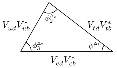
   Figure 1: Unitarity triangle $\Delta_{2}$ (see Eq. (3a)). For other unitarity triangles, the sides are denoted according to Eqs. (3) and the angles carry the corresponding index $\Delta_{i}$.

3 Unitarity triangles

For the CKM matrix one can construct 6 unitarity triangles $\Delta_{i}$:
A. Obtained from the columns multiplication

$$\text{triangle }\Delta_{1}\mbox{:\quad}V_{ud}^{\phantom{*}}V_{us}^{*}+V_{cd}^{\phantom{*}}V_{cs}^{*}+V_{td}^{\phantom{*}}V_{ts}^{*}=0,$$ (3a)

$$\text{triangle }\Delta_{2}\mbox{:\quad}V_{ud}^{\phantom{*}}V_{ub}^{*}+V_{cd}^{\phantom{*}}V_{cb}^{*}+V_{td}^{\phantom{*}}V_{tb}^{*}=0,$$

$$\text{triangle }\Delta_{3}\mbox{:\quad}V_{us}^{\phantom{*}}V_{ub}^{*}+V_{cs}^{\phantom{*}}V_{cb}^{*}+V_{ts}^{\phantom{*}}V_{tb}^{*}=0,$$

B. Obtained from the rows multiplication

$$\text{triangle }\Delta_{4}\mbox{:\quad}V_{ud}^{\phantom{*}}V_{cd}^{*}+V_{us}^{\phantom{*}}V_{cs}^{*}+V_{ub}^{\phantom{*}}V_{cb}^{*}=0,$$ (3b)

$$\text{triangle }\Delta_{5}\mbox{:\quad}V_{ud}^{\phantom{*}}V_{td}^{*}+V_{us}^{\phantom{*}}V_{ts}^{*}+V_{ub}^{\phantom{*}}V_{tb}^{*}=0,$$

$$\text{triangle }\Delta_{6}\mbox{:\quad}V_{cd}^{\phantom{*}}V_{td}^{*}+V_{cs}^{\phantom{*}}V_{ts}^{*}+V_{cb}^{\phantom{*}}V_{tb}^{*}=0.$$

From the unitarity of the CKM matrix it follows that all the unitarity triangles have the same area which is equal to $J/2$, where $J$ is the Jarlskog invariant[13, 14].

The angles of the unitarity triangles are not independent and there are simple relations that follow directly from the construction of the unitarity triangles. Let us consider as an example the angles $\phi_{1}^{\Delta_{1}}$ and $\phi_{3}^{\Delta_{6}}$

$$\phi_{1}^{\Delta_{1}} =-\arg\left(\frac{V_{td}^{\phantom{*}}V_{ts}^{*}}{V_{cd}^{\phantom{*}}V_{cs}^{*}}\right)=-\arg\left(V_{td}^{\phantom{*}}V_{ts}^{*}V_{cd}^{*}V_{cs}^{\phantom{*}}\right),$$ (4a)

$$\phi_{3}^{\Delta_{6}} =-\arg\left(\frac{V_{cs}^{\phantom{*}}V_{ts}^{*}}{V_{cd}^{\phantom{*}}V_{td}^{*}}\right)=-\arg\left(V_{cs}^{\phantom{*}}V_{ts}^{*}V_{cd}^{*}V_{td}^{\phantom{*}}\right)$$ (4b)

and we see that these two angles are equal. In the same way [15, 16] we derive the following set of the relations

$$\phi_{1}^{\Delta_{4}} =\phi_{3}^{\Delta_{3}},\quad \phi_{2}^{\Delta_{4}} =\phi_{3}^{\Delta_{2}},\quad \phi_{3}^{\Delta_{4}} =\phi_{3}^{\Delta_{1}},$$ (5)

$$\phi_{1}^{\Delta_{5}} =\phi_{2}^{\Delta_{3}}, \phi_{2}^{\Delta_{5}} =\phi_{2}^{\Delta_{2}}, \phi_{3}^{\Delta_{5}} =\phi_{2}^{\Delta_{1}}$$

$$\phi_{1}^{\Delta_{6}} =\phi_{1}^{\Delta_{3}}, \phi_{2}^{\Delta_{6}} =\phi_{1}^{\Delta_{2}}, \phi_{3}^{\Delta_{6}} =\phi_{1}^{\Delta_{1}}.$$

Thus the angles of the unitarity triangles $\Delta_{4}$, $\Delta_{5}$, $\Delta_{6}$, derived by the multiplication of the rows, can be obtained from the angles of the triangles $\Delta_{1}$, $\Delta_{2}$, $\Delta_{3}$, derived by the multiplication of the columns of the CKM matrix.

The angles of the unitarity triangles were measured only for the triangle $\Delta_{2}$ and their experimental values $\phi_{i}^{\text{exp}}$ are [10]:

$$\sin(2\phi_{1}^{\text{exp}})=0.699\pm 0.017,\quad\phi_{2}^{\text{exp}}=(84.9\pm 5.1)^{\circ}\quad\phi_{3}^{\text{exp}}=(72.1\pm 4.5)^{\circ}$$ (6)

and the lengths of the sides of all the triangles $\Delta_{i}$ can be calculated from the experimentally known absolute values of the CKM matrix elements which are equal to [10]:

$$\absolutevalue{V_{ud}^{\text{exp}}} =0.97370\pm 0.00014,\quad \absolutevalue{V_{us}^{\text{exp}}}=0.2245\pm 0.0008,$$ (7)

$$\absolutevalue{V_{ub}^{\text{exp}}} =(3.82\pm 0.24)\times 10^{-3}, \absolutevalue{V_{cd}^{\text{exp}}}=0.221\pm 0.004,$$

$$\absolutevalue{V_{cs}^{\text{exp}}} =0.987\pm 0.012, \absolutevalue{V_{cb}^{\text{exp}}}=(41.0\pm 1.4)\times 10^{-3},$$

$$\absolutevalue{V_{td}^{\text{exp}}} =(8.0\pm 0.3)\times 10^{-3}, \absolutevalue{V_{ts}^{\text{exp}}}=(38.8\pm 1.1)\times 10^{-3},$$

$$\absolutevalue{V_{tb}^{\text{exp}}} =1.013\pm 0.03$$

From the values in Eq. (7) we obtain the lengths of the sides of the unitarity triangles, given in Table 1.

Triangle	$l_{1}$	$l_{2}$	$l_{3}$
$\Delta_{1}$	$0.21860\pm 0.00078$	$0.2181\pm 0.0046$	$(3.10\pm 0.15)\times 10^{-4}$
$\Delta_{2}$	$(3.72\pm 0.23)\times 10^{-3}$	$(9.06\pm 0.35)\times 10^{-3}$	$(8.10\pm 0.39)\times 10^{-3}$
$\Delta_{3}$	$(8.58\pm 0.54)\times 10^{-4}$	$0.0405\pm 0.0015$	$0.0393\pm 0.0011$
$\Delta_{4}$	$0.2152\pm 0.0039$	$0.2216\pm 0.0026$	$(1.56\pm 0.11)\times 10^{-4}$
$\Delta_{5}$	$(7.79\pm 0.29)\times 10^{-3}$	$(8.71\pm 0.25)\times 10^{-3}$	$(3.87\pm 0.27)\times 10^{-3}$
$\Delta_{6}$	$(1.77\pm 0.07)\times 10^{-3}$	$(3.83\pm 0.11)\times 10^{-2}$	$(4.15\pm 0.19)\times 10^{-2}$

Table 1: The lengths of the sides of the unitarity triangles, defined in Eqs. (3).

The triangle inequality

$$\absolutevalue{l_{2}-l_{3}}\leq l_{1}\leq(l_{2}+l_{3}).$$ (8)

is the test that the set of the lengths $\{l_{1},l_{2},l_{3}\}$ forms a triangle. If we check whether the central values of $l_{i}$ in Table 1 form a triangle and fulfill the triangle inequality in Eq. (8), then only the triangles $\Delta_{2}$ and $\Delta_{5}$ fulfill these conditions. The angles $\phi_{k}^{\Delta_{i}}$ for these triangles are equal

$$\phi_{1}^{\Delta_{2}}=(24.21\pm 2.15)^{\circ},\;\phi_{2}^{\Delta_{2}}=(92.46\pm 10.12)^{\circ},\;\phi_{3}^{\Delta_{2}}=(63.32\pm 9.99)^{\circ},$$ (9)

$$\phi_{1}^{\Delta_{5}}=(63.41\pm 9.12)^{\circ},\;\phi_{2}^{\Delta_{5}}=(90.21\pm 9.09)^{\circ},\;\phi_{3}^{\Delta_{5}}=(26.37\pm 2.25)^{\circ}.$$

From Table 1 and Eqs. (9) one can see that the angles and the side lengths of the triangles $\Delta_{2}$ and $\Delta_{5}$ are very close and this could be expected from the fact that the deviations from the symmetry of the CKM matrix are small. From (5) one knows that unitarity implies that $\phi_{2}^{\Delta_{2}}=\phi_{2}^{\Delta_{5}}$ and within an error it is indeed a case.

The fact that the triangle inequality (8) is not fulfilled by the central values $l_{i}$ of the triangles $\Delta_{1}$, $\Delta_{3}$, $\Delta_{4}$ and $\Delta_{6}$ (see also the figures of the unitarity triangles in [17]) cannot be interpreted as a violation of the unitarity of the CKM matrix, because Eqs. (8) are fulfilled by these triangles within one standard deviation.

4 Analysis of the triangles $\Delta_{2}$ and $\Delta_{5}$

Let us now discuss in more detail the unitarity triangles $\Delta_{2}$ and $\Delta_{5}$. From Section 3 we know that the experimental information about $\Delta_{2}$ consists of the lengths $l_{i}$ of the sides of the triangle, given in Table 1 and of the angles $\phi_{i}^{\Delta_{2}}=\phi_{i}^{\text{exp}}$, given in Eq. (6). This means that there are 6 experimental data for 3 degrees of freedom. We will analyze the compatibility of the data by taking the experimental input for $\phi_{i}^{\text{exp}}$ and $\Delta\phi_{i}^{\text{exp}}$ from Eq. (6) and for $l_{i}^{\text{exp}}$, $\Delta l_{i}^{\text{exp}}$ from Table 1 and minimizing the function $\chi^{2}$

$$\chi^{2}=\quantity(\frac{\sin(2\phi_{1})-\sin(2\phi_{1}^{\text{exp}})}{\Delta\sin(2\phi_{1}^{\text{exp}})})^{2}+\quantity(\frac{\phi_{2}-\phi_{2}^{\text{exp}}}{\Delta\phi_{2}^{\text{exp}}})^{2}+\quantity(\frac{\phi_{3}-\phi_{3}^{\text{exp}}}{\Delta\phi_{3}^{\text{exp}}})^{2}\\ +\quantity(\frac{l_{1}-l_{1}^{\text{exp}}}{\Delta l_{1}^{\text{exp}}})^{2}+\quantity(\frac{l_{2}-l_{2}^{\text{exp}}}{\Delta l_{2}^{\text{exp}}})^{2}+\quantity(\frac{l_{3}-l_{3}^{\text{exp}}}{\Delta l_{3}^{\text{exp}}})^{2}$$ (10)

with respect to the $l_{1}$, $l_{2}$, $l_{3}$. The values of the fitted parameters are

$$l_{1} =(3.45\pm 0.09)\times 10^{-3},$$ (11)

$$l_{2} =(8.99\pm 0.16)\times 10^{-3},$$

$$l_{3} =(8.50\pm 0.18)\times 10^{-3}$$

and the value of the $\chi^{2}$ and the p-value of the fit are

$$\chi^{2}=2.91,\quad\text{{p}-value}=0.41$$ (12)

so the experimental data for the triangle $\Delta_{2}$ are compatible with the assumption that $l_{1}^{\text{exp}}$, $l_{2}^{\text{exp}}$ and $l_{3}^{\text{exp}}$ form a triangle, whose angles are $\phi_{1}^{\text{exp}}$, $\phi_{2}^{\text{exp}}$ and $\phi_{3}^{\text{exp}}$.

The triangle $\Delta_{2}$ thus obtained, whose lengths of the sides $l_{i}$ are given in Eq. (11) has the following values of the angles

$$\phi_{1}^{\Delta_{2}} =(22.54\pm 0.72)^{\circ},$$ (13)

$$\phi_{2}^{\Delta_{2}} =(86.77\pm 4.1)^{\circ},$$

$$\phi_{3}^{\Delta_{2}} =(70.69\pm 3.9)^{\circ}.$$

By comparing the values of the lengths given in Eqs. (11) with those of Table 1 we note that the errors are significantly reduced. The error reduction also occurs for the values of angles in Eqs. (13) and (9).

The analysis for the triangle $\Delta_{2}$ cannot be applied for the remaining triangles, because their angles have not been measured. Additionally the lengths of the sides of some of the triangles violate the triangle inequality Eq. (8), so strictly speaking they do not form the triangles. To improve this situation we apply two additional constraints in the fit of the lengths of the sides for those triangles:

$$\left.\parbox{368.57964pt}{ \begin{enumerate} \par\enumerate@item@The range of the fitted values of the lengths have to fulfill the triangle inequality Eq.~{}\eqref{eq:4}. \par\enumerate@item@The area of the fitted triangle has to be equal to the area for the triangle $\Delta_{2}$, which is equal \begin{equation*}\text{Area of the triangle $\Delta_{2}$}=(1.464\pm 0.048)\times 10^{-5}.\end{equation*} \par\end{enumerate}}\quad\right\}$$

Such a fit gives the following result for the lengths of the sides of triangle $\Delta_{5}$

$$l_{1} =(7.75^{+0.18}_{-0.17})\times 10^{-3},$$ (15)

$$l_{2} =(8.71\pm 0.25)\times 10^{-3},$$

$$l_{3} =(3.80^{+0.12}_{-0.10})\times 10^{-3}$$

and the value of the $\chi^{2}$ and the p-value of the fit are

$$\chi^{2}=0.112,\quad\text{{p}-value}=0.262.$$ (16)

From the values in Eq. (15) we obtain the angles of the triangle $\Delta_{5}$

$$\phi_{1}^{\Delta_{5}}=(62.71\pm 4.4)^{\circ},\quad\phi_{2}^{\Delta_{5}}=(91.46\pm 5.2)^{\circ},\quad\phi_{3}^{\Delta_{5}}=(25.82\pm 1.2)^{\circ}.$$ (17)

Eqs. (13) and (17) demonstrate that the fitted values of the angles are compatible with the relation $\phi_{2}^{\Delta_{2}}=\phi_{2}^{\Delta_{5}}$ in Eq. (5) and the errors are reduced.

5 Analysis of the remaining triangles

The lengths of the sides

For the triangles $\Delta_{1}$, $\Delta_{3}$, $\Delta_{4}$, and $\Delta_{6}$ we know only the lengths of the sides, given in Table 1 and the angles have not been measured, so the situation is similar as in the case of the triangle $\Delta_{5}$, so we use the additional constraints described in Eq. (4) for the determination of the lengths $l_{i}$. The results of the fits are given in Tables 2 and 3.

Triangle $\Delta_{1}$	Triangle $\Delta_{3}$
$l_{1}=0.21859\pm(2.5\times 10^{-6})$	$l_{1}=(8.55\pm 0.34)\times 10^{-4}$
$l_{2}=0.21831\pm(2.5\times 10^{-6})$	$l_{2}=(3.946\pm 0.009)\times 10^{-2}$
$l_{3}=(3.104\pm 0.023)\times 10^{-4}$	$l_{3}=(3.988\pm 0.009)\times 10^{-2}$
Triangle $\Delta_{4}$	Triangle $\Delta_{6}$
$l_{1}=0.21967^{+0.000022}_{-0.00018}$	$l_{1}=(1.77\pm 0.01)\times 10^{-3}$
$l_{2}=0.21959^{+0.00018}_{-0.000022}$	$l_{2}=(3.875\pm 0.002)\times 10^{-2}$
$l_{3}=(1.565\pm 0.85)\times 10^{-5}$	$l_{3}=(4.035\pm 0.002)\times 10^{-2}$

Table 2: The results of the fit of the unitarity triangles.

Triangle	$\chi^{2}$	p-value
$\Delta_{1}$	0.0016	0.032
$\Delta_{3}$	0.75	0.386
$\Delta_{4}$	1.91	0.166
$\Delta_{6}$	0.54	0.462

Table 3: The values of $\chi^{2}$ and the p-values of the fits for the unitarity triangles.

Angles of the triangles

From Table 2 we can see that the lengths of the sides $l_{1}$ and $l_{2}$ of the triangles $\{\Delta_{1},\Delta_{4}\}$ are very close and it is also true for the pair of the sides $l_{2}$ and $l_{3}$ of the triangles $\{\Delta_{3},\Delta_{6}\}$. What is more important for each triangle $\Delta_{i}$, $i=1,3,4,6$ one side is much shorter than two remaining ones. This causes that the smallest angle is determined more precisely than the remaining ones and one can see that the values of those angles in Table 4 are compatible with the relations in Eq. (5). The fitted values of the angles are given in Table 4.

Triangle $\Delta_{1}$	Triangle $\Delta_{3}$
$\phi_{1}=(154.3\pm 1.8)^{\circ}$	$\phi_{1}=(1.07\pm 0.12)^{\circ}$
$\phi_{2}=(25.7\pm 1.8)^{\circ}$	$\phi_{2}=(59.9\pm 10.1)^{\circ}$
$\phi_{3}=(0.0352\pm 0.0024)^{\circ}$	$\phi_{3}=(119.1\pm 10.1)^{\circ}$
Triangle $\Delta_{4}$	Triangle $\Delta_{6}$
$\phi_{1}=(120.9\pm 62.2)^{\circ}$	$\phi_{1}=(1.03\pm 1.02)^{\circ}$
$\phi_{2}=(59.1\pm 62.2)^{\circ}$	$\phi_{2}=(23.1\pm 24.1)^{\circ}$
$\phi_{3}=(0.035\pm 0.022)^{\circ}$	$\phi_{3}=(155.9\pm 25.1)^{\circ}$

Table 4: The angles of the unitarity triangles, obtained from the fitted values of the sides of the triangles.

6 Summary and conclusions

We have examined all the unitarity triangles of the CKM matrix and analyzed their properties. Our analysis is independent of the parameterization of the CKM matrix and it is based on the properties of the unitarity triangles that follow from the SM.

There are two types of the SM predictions concerning the unitarity triangles:

1. The unitarity of the CKM matrix implies

   $$\phi_{1}^{\Delta_{i}}+\phi_{2}^{\Delta_{i}}+\phi_{3}^{\Delta_{i}}=180^{\circ}$$ (18)

   and it it involves the angles of only one unitarity triangle.

2. The other type of the relations, given in Eqs. (5), involve the angles of different unitarity triangles.

Relation of Type 1 given by Eq. (18) is a test of the unitarity of the CKM matrix and it is tested for one unitarity triangle and is well satisfied by the experimental data [10] .

Relations of Type 2 given in Eqs. (5) follow from the structure of the SM and they do not depend on the specific properties of the CKM matrix, like unitarity. If the CKM matrix exists, then Eqs. (5) have to be fulfilled. On the other hand, if any of the relations in Eqs. (5) are not experimentally fulfilled, then the description of of the flavour-changing weak interaction by the CKM matrix is invalid! It should be stressed that relations (5) constitute a very powerful test of the SM. If any pair of angles in those relations is measured and they are not equal, then the whole SM has to be revised.

Our derivation of the values of the angles of the unitarity triangles assumed the existence of the CKM matrix so the consistency of our results for the unitarity angles in Eqs. (13), (17) and Table 4 is just the consistency of our procedure and calculations.

An important element of our procedure, which we call the Method A was the assumption that the area of all unitarity triangles is the same. This fact follows from the unitarity of the CKM matrix. The experimental input that we use consists of the well established absolute values of the CKM matrix elements and the angles of the $\Delta_{2}$ triangle. This information and the equality of the area of all unitarity triangles allowed us to determine the lengths of the sides and the angles of all the unitarity triangles.

The alternative way, which we call the Method B of the determination of all the unitarity triangles is to use the values of the fitted parameters of the CKM matrix [10]

$$\sin\theta_{12} =0.22650\pm 0.00048,\quad \sin\theta_{13} =0.00361^{+0.00011}_{-0.00009},$$ (19)

$$\sin\theta_{23} =0.04053^{+0.00083}_{-0.00061}, \delta =1.196^{+0.045}_{-0.043}.$$

and then to directly obtain the angles of the unitarity triangles from the standard parameterization [10, 18] of the CKM matrix.

Triangle	angle	Method A	Method B
	$\phi_{1}$	$(154.3\pm 1.8)^{\circ}$	–
$\Delta_{1}$	$\phi_{2}$	$(25.7\pm 1.8)^{\circ}$	–
	$\phi_{3}$	$(0.0352\pm 0.0024)^{\circ}$	–
	$\phi_{1}$	$(22.54\pm 0.72)^{\circ}$	$(22.53\pm 2.55)^{\circ}$
$\Delta_{2}$	$\phi_{2}$	$(86.77\pm 4.1)^{\circ}$	$(88.98\pm 5.13)^{\circ}$
	$\phi_{3}$	$(70.69\pm 3.9)^{\circ}$	$(68.49\pm 4.31)^{\circ}$
	$\phi_{1}$	$(1.07\pm 0.12)^{\circ}$	–
$\Delta_{3}$	$\phi_{2}$	$(59.9\pm 10.1)^{\circ}$	$(67.43\pm 44.7)^{\circ}$
	$\phi_{3}$	$(119.1\pm 10.1)^{\circ}$	$(111.47\pm 47.2)^{\circ}$
	$\phi_{1}$	$(120.9\pm 62.2)^{\circ}$	–
$\Delta_{4}$	$\phi_{2}$	–	–
	$\phi_{3}$	$(0.035\pm 0.022)^{\circ}$	–
	$\phi_{1}$	$(62.71\pm 4.4)^{\circ}$	$(67.43\pm 1.56)^{\circ}$
$\Delta_{5}$	$\phi_{2}$	$(91.46\pm 5.2)^{\circ}$	$(88.98\pm 35.8)^{\circ}$
	$\phi_{3}$	$(25.82\pm 1.2)^{\circ}$	–
	$\phi_{1}$	$(1.04\pm 0.81)^{\circ}$	–
$\Delta_{6}$	$\phi_{2}$	$(23.5\pm 19.2)^{\circ}$	–
	$\phi_{3}$	$(155.5\pm 20.0)^{\circ}$	–

Table 5: Comparison of the angles of the unitarity triangles obtained by two methods. Method A is the one used in this paper and the Method B is the direct calculation from the standard parameterization of the CKM matrix. The entries “–” mean that the calculated error was larger than the calculated value.

In Table 5 we compare the angles of the unitarity triangles, which were obtained with our method (Method A) and by the direct approach (Method B) and we see that the Method B produces very limited results: one can fully determine only one unitarity triangle and two angles of the triangles $\Delta_{3}$ and $\Delta_{5}$. It should be noted that the predictions of both methods coincide (within one standard deviation) for the available angles. The experimental values for the angles of the $\Delta_{2}$ triangle also are equal (within one standard deviation) to the predictions of those angles. The fit of the triangle $\Delta_{4}$, with $\chi^{2}=1.91$ presents some tension with the existing experimental data.

The progress in the experimental situation and a possibility of a measurement of the triangle $\Delta_{5}$ can be brought in the $B$-meson experiments [19] at KEK with the Belle II detector [20] or at CERN with the LHCb detector [21, 22]. Also the theoretical analysis like [23] on removing tensions present in the present data may bring an important advance in our knowledge of the CKM matrix.

Any deviation from the predicted values of the angles would be a sign of the violation of the CKM matrix unitarity and a confirmation of the $3\sigma$ tension [10] for the unitarity prediction for the first row of the CKM matrix and any violation of the relations in Eq. (5) would be a sign of a serious contradiction with predictions of the SM.