KL-Entropy-Regularized RL with a
Generative Model is Minimax Optimal

Abstract

In this work, we consider and analyze the sample complexity of model-free reinforcement learning with a generative model. Particularly, we analyze mirror descent value iteration (MDVI) by Geist et al. (2019) and Vieillard et al. (2020a), which uses the Kullback-Leibler divergence and entropy regularization in its value and policy updates. Our analysis shows that it is nearly minimax-optimal for finding an $\varepsilon$-optimal policy when $\varepsilon$ is sufficiently small. This is the first theoretical result that demonstrates that a simple model-free algorithm without variance-reduction can be nearly minimax-optimal under the considered setting.

1 Introduction

In the generative model setting, the agent has access to a simulator of a Markov decision process (MDP), to which the agent can query next states of arbitrary state-action pairs (Azar et al., 2013). The agent seeks a near-optimal policy using as small number of queries as possible.

While the generative model setting is simpler than the online reinforcement learning (RL) setting, proof techniques developed under this setting often generalize to more complex settings. For example, the total-variance technique developed by Azar et al. (2013) and Lattimore & Hutter (2012) is now an indispensable tool for a sharp analysis of RL algorithms in the online RL setting for tabular MDP (Azar et al., 2017; Jin et al., 2018) and linear function approximation (Zhou et al., 2021).

In this paper, we consider a model-free approach for the generative model setting with tabular MDP. Particularly, we analyze mirror descent value iteration (MDVI) by Geist et al. (2019) and Vieillard et al. (2020a), which uses Kullback-Leibler (KL) divergence and entropy regularization in its value and policy updates. We prove its near minimax-optimal sample complexity for finding an $\varepsilon$-optimal policy when $\varepsilon$ is sufficiently small. Our result and analysis have the following consequences.

First, we demonstrate the effectiveness of KL and entropy regularization. There are some previous works that argue the benefit of regularization from a theoretical perspective in value-iteration-like algorithms (Kozuno et al., 2019; Vieillard et al., 2020a, b) and policy optimizaiton (Mei et al., 2020; Cen et al., 2021; Lan, 2022). Compared to those works, we show that simply combining value iteration with regularization achieves the near minimax-optimal sample complexity.

Second, as discussed by Vieillard et al. (2020a), MDVI encompasses various algorithms as special cases or equivalent forms. While we do not analyze each algorithm, most of them are minimax-optimal too in the generative model setting with tabular MDP.

Lastly and most importantly, MDVI uses no variance-reduction technique, in contrast to previous model-free approaches (Sidford et al., 2018; Wainwright, 2019; Khamaru et al., 2021). Consequently, our analysis is straightforward, and it would be easy to extend it to more complex settings, such as the online RL and linear function approximation. Furthermore, previous approaches need pessimism to obtain a near-optimal policy, which prevents them from being extended to the online RL setting, where the optimism plays an important role for an efficient exploration (Azar et al., 2017; Jin et al., 2018). On the other hand, MDVI is compatible with optimism. Our analysis paves the way for the combination of online exploration techniques with minimax model-free algorithms.

2 Related work

Write $\gamma$, $H$, $X$, and $A$ for the discount factor, effective horizon $\frac{1}{1-\gamma}$, and number of states and actions.

Learning with a generative model

In the generative model setting, there are two problem settings: finding (i) an $\varepsilon$-optimal Q-value function with probability at least $1-\delta$, and (ii) an $\varepsilon$-optimal policy with probability at least $1-\delta$, where $\delta\in(0,1)$, and $\varepsilon>0$. Both problems are known to have sample complexity lower bounds of $\Omega(XAH^{3}/\varepsilon^{2})$ (Azar et al., 2013; Sidford et al., 2018). Note that even if an $\varepsilon$-optimal Q-value function is obtained, additional data and computation are necessary to find an $\varepsilon$-optimal policy (Sidford et al., 2018). In this paper, we consider the learning of an $\varepsilon$-optimal policy.

There exist minimax-optimal model-based algorithms for learning a near-optimal value function (Azar et al., 2013) and policy (Agarwal et al., 2020; Li et al., 2020). Also, there exist minimax-optimal model-free algorithms for learning a near-optimal value function (Wainwright, 2019; Khamaru et al., 2021; Li et al., 2021b) and policy (Sidford et al., 2018). While model-based algorithms are conceptually simple, they have a higher computational complexity than that of model-free algorithms. The algorithm (MDVI) we analyze in this paper is a model-free algorithm for finding a near-optimal policy, and has a low computational complexity.

Arguably, Q-learning is one of the simplest model-free algorithms (Watkins & Dayan, 1992; Even-Dar et al., 2003). Unfortunately, Li et al. (2021a) provide a tight analysis of Q-learning and show that its sample complexity is $\widetilde{\mathcal{O}}(XAH^{4}/\varepsilon^{2})$ for finding an $\varepsilon$-optimal Q-value function, which is one $H$ factor away from the lower bound. To remove the extra $H$ factor, some works (Sidford et al., 2018; Wainwright, 2019; Khamaru et al., 2021) leverage variance reduction techniques. While elegant, variance reduction techniques lead to multi-epoch algorithms with involved analyses. In contrast, MDVI requires no variance reduction and is significantly simpler.

MDVI’s underlying idea that enables such simplicity is, while implicit, the averaging of value function estimates. Li et al. (2021b) shows that averaging Q-functions computed in Q-learning can find a near-optimal Q-function with a minimax-optimal sample complexity. Azar et al. (2011) also provides a simple algorithm called Speedy Q-learning (SQL), which performs the averaging of value function estimates. In fact, as argued in (Vieillard et al., 2020a), SQL is equivalent to a special case of MDVI with only KL regularization. While previous works on MDVI (Vieillard et al., 2020a) and an equivalent algorithm called CVI (Kozuno et al., 2019) provide error propagation analyses, they do not provide sample complexity. This paper proves the first nearly minimax-optimal sample complexity bound for MDVI-type algorithm. We tighten previous results by (i) using the entropy regularization, which speeds up the convergence rate, (ii) improved error propagation analyses (Lemmas 1 and 9), and (iii) careful application of the total variance technique (Azar et al., 2013).

In addition to the averaging, Theorem 1 is based on the idea of using a non-stationary policy (Scherrer & Lesner, 2012). While the last policy of MDVI is near-optimal when $\varepsilon$ is small, a non-stationary policy constructed from policies outputted by MDVI is near-optimal for a wider range of $\varepsilon$.

Range of Valid $\varepsilon$

Although there are multiple minimax-optimal algorithms for the generative model setting, there ranges of valid $\varepsilon$ differ. The model-based algorithm by Azar et al. (2013) is nearly minimax-optimal for $\varepsilon\leq\sqrt{H/X}$, which is later improved to $\sqrt{H}$ by Agarwal et al. (2020), and to $H$ by Li et al. (2020). As for model-free approaches, the algorithm by Sidford et al. (2018) is nearly minimax-optimal for $\varepsilon\leq 1$. MDVI is nearly minimax-optimal for $\varepsilon\leq 1/\sqrt{H}$ (non-stationary policy case, Theorem 1) and $\varepsilon\leq 1/H$ (last policy case, Theorem 2). Therefore, it has one of the narrowest range of valid $\varepsilon$ (second worst) compared to other algorithms. It is unclear if this is an artifact of our analysis or the real limitation of MDVI-type algorithm. We leave this topic as a future work.

Regularization in MDPs

Sometimes, regularization is added to the reward to encourage exploration in MDPs (Fox et al., 2016; Vamplew et al., 2017). In recent years, Neu et al. (2017); Geist et al. (2019); Lee et al. (2018); Yang et al. (2019) have provided a unified framework for regularized MDPs. Specifically, Geist et al. (2019) propose the Regularized Modified Policy Iteration algorithm and Mirror Descent Modified Policy Iteration to solve regularized MDPs. In the meantime, Vieillard et al. (2020a) provide theoretical guarantees of KL-regularized value iteration in the approximate setting. Particularly, they show that KL regularization results in the averaging of Q-value functions and show that the averaging leads to an improved error propagation result. We extend their improved error propagation result to a KL- and entropy- regularization case. Our results provide theoretical underpinnings to many regularized RL algorithms in Vieillard et al. (2020a, Table 1) and a high-performing deep RL algorithm called Munchausen DQN (Vieillard et al., 2020b).

3 Preliminaries

For a set $\mathbf{S}$, we denote its complement as $\mathbf{S}^{c}$. For a positive integer $N$, we let $\left[N\right]\vcentcolon\nolinebreak\mkern-1.2mu=\{1,\ldots,N\}$. Without loss of generality, every finite set is assumed to be a subset of integers. For a finite set, say $\mathbf{S}$, the set of probability distributions over $\mathbf{S}$ is denoted by $\Delta(\mathbf{S})$. For a vector $v\in\mathbf{R}^{M}$, its $m$-th element is denoted by $v_{m}$ or $v(m)$. We let $\mathbf{1}\vcentcolon\nolinebreak\mkern-1.2mu=(1,\ldots,1)^{\top}$ and $\mathbf{0}\vcentcolon\nolinebreak\mkern-1.2mu=(0,\ldots,0)^{\top}$, whose dimension will be clear from the context. For a matrix $A\in\mathbf{R}^{N\times M}$, we denote its $n$-th row and $m$-th value of the $n$-th row by $A_{n}$ and $A_{n}^{m}$, respectively. The expectation and variance of a random variable $X$ are denoted as $\mathbb{E}[X]$ and $\mathbb{V}[X]$, respectively. The empty sum is defined to be $0$, e.g., $\sum_{i=j}^{k}a_{i}=0$ if $j>k$.

We consider a Markov Decision Process (MDP) defined by $\left\lparen\mathbf{X},\mathbf{A},\gamma,r,P\right\rparen$, where $\mathbf{X}$ is the state space of size $X$, $\mathbf{A}$ the action space of size $A$, $\gamma\in[0,1)$ the discount factor, $r\in[-1,1]^{XA}$ the reward vector with $r_{x,a}$ denoting the reward when taking an action $a$ at a state $x$, and $P\in\mathbf{R}^{XA\times X}$ state transition probability matrix with $P_{x,a}^{y}$ denoting the state transition probability to a new state $y$ from a state $x$ when taking an action $a$. We let $H$ be the (effective) time horizon $1/(1-\gamma)$.

Note that $(Pv)(x,a)=E\left[v(X_{1})\middle|X_{0}=x,A_{0}=a\right]$ for any $v\in\mathbf{R}^{X}$. Any policy $\pi$ is identified as a matrix $\pi\in\mathbf{R}^{X\times XA}$ such that $(\pi q)(x):=\sum_{a\in\mathbf{A}}\pi(a|x)q\left\lparen x,a\right\rparen$ for any $q\in\mathbf{R}^{XA}$. For convenience, we adopt a shorthand notation, $P^{\pi}:=P\pi$. With these notations, the Bellman operator $T^{\pi}$ for a policy $\pi$ is defined as an operator such that $T^{\pi}q:=r+\gamma P^{\pi}q$. The Q-value function $q^{\pi}$ for a policy $\pi$ is its unique fixed point. The state-value function $v^{\pi}$ is defined as $\pi q^{\pi}$. An optimal policy $\pi_{*}$ is a policy such that $v^{*}:=v^{\pi_{*}}\geq v^{\pi}$ for any policy $\pi$, where the inequality is point-wise.

4 Mirror Descent Value Iteration and Main Results

For any policies $\pi$ and $\mu$, let $\log\pi$ and $\log\frac{\pi}{\mu}$ be the functions $x,a\mapsto\log\pi(a|x)$ and $x,a\mapsto\log\frac{\pi(a|x)}{\mu(a|x)}$ over $\mathbf{X}\times\mathbf{A}$. We analyze (approximate) MDVI whose update is the following (Vieillard et al., 2020a):

$$q_{k+1}=r+\gamma Pv_{k}+\varepsilon_{k}\,,$$ (1)

where $v_{k}\vcentcolon\nolinebreak\mkern-1.2mu=\pi_{k}\left\lparen q_{k}-\tau\log\dfrac{\pi_{k}}{\pi_{k-1}}-\kappa\log\pi_{k}\right\rparen$,

$$\pi_{k}\left\lparen\cdot\middle|x\right\rparen=\operatorname*{arg\,max}_{p\in\Delta(\mathbf{A})}\sum_{a\in\mathbf{A}}p(a)\left\lparen q_{k}(s,a)-\tau\log\frac{p(a)}{\pi_{k-1}\left\lparen a\middle|x\right\rparen}-\kappa\log p(a)\right\rparen$$ (2)

for all $x\in\mathbf{X}$, and $\varepsilon_{k}:\mathbf{X}\times\mathbf{A}\rightarrow\mathbf{R}$ is an “error” function, which abstractly represents the deviation of $q_{k+1}$ from the update target $r+\gamma Pv_{k}$. In other words, MDVI is value iteration with KL and entropy regularization.

Let $s_{k}\vcentcolon\nolinebreak\mkern-1.2mu=q_{k}+\alpha s_{k-1}=\sum_{j=0}^{k-1}\alpha^{j}q_{k-j}$. The policy (2) can be rewritten as a Boltzmann policy of $s_{k}$, i.e., $\pi_{k}(a|x)\propto\exp\left\lparen\beta s_{k}(x,a)\right\rparen$, where $\alpha\vcentcolon\nolinebreak\mkern-1.2mu=\tau/(\tau+\kappa)$, and $\beta\vcentcolon\nolinebreak\mkern-1.2mu=1/(\tau+\kappa)$, see Appendix B for details. Substituting $\pi_{k-1}$ and $\pi_{k}$ in $v_{k}$ with this expression of the policy, we deduce that

$$v_{k}(x)=\frac{1}{\beta}\log\sum_{a\in\mathbf{A}}\exp\left\lparen\beta s_{k}(x,a)\right\rparen-\frac{\alpha}{\beta}\log\sum_{a\in\mathbf{A}}\exp\left\lparen\beta s_{k-1}(x,a)\right\rparen\,.$$ (3)

Thus, letting $w_{k}$ be the function $x\mapsto\beta^{-1}\log\sum_{a\in\mathbf{A}}\exp\left\lparen\beta s_{k}(x,a)\right\rparen$ over $\mathbf{X}$, MDVI’s update rules can be equivalently written as

$$q_{k+1}=r+\gamma P\left\lparen w_{k}-\alpha w_{k-1}\right\rparen+\varepsilon_{k}\text{ and }\pi_{k}\mathopen{\lparen}a\mathord{|}x\mathclose{\rparen}\propto\exp\left\lparen\beta s_{k}(x,a)\right\rparen\text{ for all }(x,a)\in\mathbf{X}\times\mathbf{A}\,.$$ (4)

A sample-approximate version of MDVI shown in Algorithm 1 (MDVI) uses this equivalent form of MDVI. Furthermore, for simplicity of the analysis, we consider the limit of $\tau,\kappa\to 0$ while keeping $\alpha=\tau/(\tau+\kappa)$ to a constant value (which corresponds to letting $\beta\to\infty$).

Input: $\alpha\in[0,1)$, number of iterations $K$, and number of next-state samples per iteration $M$.

Let $s_{0}=\mathbf{0}\in\mathbf{R}^{XA}$ and $w_{0}=w_{-1}=\mathbf{0}\in\mathbf{R}^{X}$;

for $k$ from $0$ to $K-1$ do

       Let $v_{k}=w_{k}-\alpha w_{k-1}$;

       for each state-action pair $\left\lparen x,a\right\rparen\in\mathbf{X}\times\mathbf{A}$ do

             Sample $(y_{k,m,x,a})_{m=1}^{M}$ from the generative model $P(\cdot|x,a)$;

             Let $q_{k+1}(x,a)=r(x,a)+\gamma M^{-1}\sum_{m=1}^{M}v_{k}(y_{k,m,x,a})$;

            

       end for

      Let $s_{k+1}=q_{k+1}+\alpha s_{k}$ and $w_{k+1}(x)=\max_{a\in\mathbf{A}}s_{k+1}(x,a)$ for each $x\in\mathbf{X}$;

      

end for

return $(\pi_{k})_{k=0}^{K}$ , where $\pi_{k}$ is greedy policy with respect to $s_{k}$;

Algorithm 1 $\hyperref@@ii[algo:mdvi]{\texttt{MDVI}}(\alpha,K,M)$

Remark 1.

Even if $\beta$ is finite, MDVI is nearly minimax-optimal as long as $\beta$ is large enough. Indeed, $\beta^{-1}\log\sum_{a\in\mathbf{A}}\exp(q(x,a))$ satisfies (Kozuno et al., 2019, Lemma 7) that

$$\max_{a\in\mathbf{A}}q(x,a)\leq\beta^{-1}\log\sum_{a\in\mathbf{A}}\exp(q(x,a))\leq\max_{a\in\mathbf{A}}q(x,a)+\beta^{-1}\log A\,.$$

Thus, while $\beta$ appears in the proofs of Theorems 1 and 2 if it is finite, it always appear as $\beta^{-1}\log A$ multiplied by $H$-dependent constant. Therefore, MDVI is nearly minimax-optimal as long as $\beta$ is large enough.

Why KL Regularization?

The weight $\alpha$ used in $s_{k}$ updates monotonically increases as the coefficient of the KL regularization $\tau$ increases. As we see later, error terms appear in upper bounds of $\mathopen{\lVert}v^{*}-v^{\pi_{k}}\mathclose{\rVert_{\infty}}$ as $(1-\alpha)\sum_{j=1}^{k}\alpha^{k-j}\varepsilon_{j}$. Applying Azuma-Hoeffiding inequality, it is approximately bounded by $H\sqrt{1-\alpha}$. Therefore, MDVI becomes more robust to sampling error as $\alpha$ increases. The KL regularization confers this benefit to the algorithm.

Why Entropy Regularization?

When there is no entropy regularization ($\alpha=1$), the convergence rate of MDVI becomes $1/K$ while it is $\alpha^{K}$ for $\gamma\leq\alpha<1$ (Vieillard et al., 2020a). In the former case, we need to set $K\approx H^{2}/\varepsilon$, whereas in the latter case, $K\approx 1/(1-\alpha)$ suffices. Since we will set $\alpha$ to either $\gamma$ or $1-(1-\gamma)^{2}$, $K\approx H$ or $H^{2}$. Thus, we can use more samples per one value update (i.e., larger $M$). A larger $M$ leads to a smaller value estimation variance ($\sigma(v_{k})$ in Lemma 6), which is important to improve the range of $\varepsilon$. Even when $\alpha=1$, MDVI is nearly minimax-optimal (proof omitted). However, $\varepsilon$ must be less than or equal to $1/H^{2}$.

Main Theoretical Results

The following theorems show the near minimax-optimality of MDVI. For a sequence of policies $(\pi_{k})_{k=0}^{K}$ outputted by MDVI, we let $\pi_{k}^{\prime}$ be the non-stationary policy that follows $\pi_{k-t}$ at the $t$-th time step until $t=k$, after which $\pi_{0}$ is followed. Note that the value function of such a non-stationary policy is given by $v^{\pi^{\prime}_{k}}=\pi_{k}T^{\pi_{k-1}}\cdots T^{\pi_{1}}q^{\pi_{0}}$.

Theorem 1.

Assume that $\varepsilon\in(0,1/\sqrt{H}]$. Then, there exist positive constants $c_{1},c_{2}\geq 1$ independent of $H$, $X$, $A$, $\varepsilon$, and $\delta$ such that when MDVI is run with the settings

$$\alpha=\gamma\,,K=\left\lceil\frac{3}{1-\alpha}\log\frac{c_{1}H}{\varepsilon}+2\right\rceil\,,\text{ and }M=\left\lceil\frac{c_{2}H^{2}}{\varepsilon^{2}}\log\frac{16KXA}{\delta}\right\rceil\,,$$ (5)

it outputs a sequence of policies $(\pi_{k})_{k=0}^{K}$ such that $\mathopen{\lVert}v^{*}-v^{\pi^{\prime}_{K}}\mathclose{\rVert_{\infty}}\leq\varepsilon$ with probability at least $1-3\delta/4$, using $\widetilde{\mathcal{O}}\left\lparen H^{3}XA/\varepsilon^{2}\right\rparen$ samples from the generative model.

Storing all policies requires the memory space of $KXA$ and can be prohibitive in some cases. The next theorem shows that the last policy outputted by MDVI is near-optimal when $\varepsilon\leq 1/H$.

Theorem 2.

Assume that $\varepsilon\in(0,1/H]$. Then, there exist positive constants $c_{3},c_{4}\geq 1$ independent of $H$, $X$, $A$, $\varepsilon$, and $\delta$ such that when MDVI is run with the settings

$$\alpha=1-(1-\gamma)^{2}\,,K=\left\lceil\frac{5}{1-\alpha}\log\frac{c_{3}H}{\varepsilon}+2\right\rceil\,,\text{ and }M=\left\lceil\frac{c_{4}H}{\varepsilon^{2}}\log\frac{16KXA}{\delta}\right\rceil\,,$$ (6)

it outputs a sequence of policies $(\pi_{k})_{k=0}^{K}$ such that $\mathopen{\lVert}v^{*}-v^{\pi_{K}}\mathclose{\rVert_{\infty}}\leq\varepsilon$ with probability at least $1-\delta$, using $\widetilde{\mathcal{O}}\left\lparen H^{3}XA/\varepsilon^{2}\right\rparen$ samples from the generative model.

5 Proofs of the Main Results

Before the proof, we introduce some notations. A table of notations is provided in Appendix A.

Notation.

$\square$ denotes an indefinite constant that changes throughout the proof and is independent of $H$, $X$, $A$, $\varepsilon$, and $\delta$. We let $A_{\gamma,k}\vcentcolon\nolinebreak\mkern-1.2mu=\sum_{j=0}^{k-1}\gamma^{k-j}\alpha^{j}$ and $A_{k}\vcentcolon\nolinebreak\mkern-1.2mu=\sum_{j=0}^{k-1}\alpha^{j}$ for any non-negative integer $k$ with $A_{\infty}\vcentcolon\nolinebreak\mkern-1.2mu=1/(1-\alpha)$. $\mathbf{F}_{k,m}$ denotes the $\sigma$-algebra generated by random variables $\{y_{j,n,x,a}|(j,n,x,a)\in[k-2]\times[M]\times\mathbf{X}\times\mathbf{A}\}\cup\{y_{j,n,x,a}|(j,n,x,a)\in\{k-1\}\times[m-1]\times\mathbf{X}\times\mathbf{A}\}$. For any $k\in\{0\}\cup[K-1]$ and $v\in\mathbf{R}^{X}$, $\mathrm{Var}(v)$ and $\widehat{P}_{k}v$ denote the functions

$$\textstyle\mathrm{Var}(v):(x,a)\mapsto(Pv^{2})(x,a)-(Pv)^{2}(x,a)\text{ and }\widehat{P}_{k}v:(x,a)\mapsto\sum_{m=1}^{M}v(y_{k,m,x,a})/M\,,$$ (7)

respectively. We often write $\sqrt{\mathrm{Var}(v)}$ as $\sigma(v)$. Furthermore, $\varepsilon_{k}$ and $E_{k}$ denote “error” functions

$$\textstyle\varepsilon_{k}:(x,a)\mapsto\gamma\widehat{P}_{k-1}v_{k-1}(x,a)-\gamma Pv_{k-1}(x,a)\text{ and }E_{k}:(x,a)\mapsto\sum_{j=1}^{k}\alpha^{k-j}\varepsilon_{j}(x,a)\,,$$ (8)

respectively. (Note that $\varepsilon_{1}=E_{1}=\mathbf{0}$ since $v_{0}=\mathbf{0}$.) For a sequence of policies $(\pi_{k})_{k\in\mathbf{Z}}$, we let $T_{j}^{i}\vcentcolon\nolinebreak\mkern-1.2mu=T^{\pi_{i}}T^{\pi_{i-1}}\cdots T^{\pi_{j+1}}T^{\pi_{j}}$ for $i\geq j$, and $T_{j}^{i}\vcentcolon\nolinebreak\mkern-1.2mu=I$ otherwise. We also let $P_{j}^{i}\vcentcolon\nolinebreak\mkern-1.2mu=P^{\pi_{i}}P^{\pi_{i-1}}\cdots P^{\pi_{j+1}}P^{\pi_{j}}$ for $i\geq j$, and $P_{j}^{i}\vcentcolon\nolinebreak\mkern-1.2mu=I$ otherwise. As a special case with $\pi_{k}=\pi_{*}$ for all $k$, we let $P_{*}^{i}\vcentcolon\nolinebreak\mkern-1.2mu=(P^{\pi_{*}})^{i}$. Finally, throughout the proof, $\iota_{1}$ and $\iota_{2}$ denotes $\log(8KXA/\delta)$ and $\log(16KXA/\delta)$, repspectively.

5.1 Proof of Theorem 1 (Near-optimality of the Non-stationary Policy)

The first step of the proof is the error propagation analysis of MDVI given below. It differs from the one of Vieillard et al. (2020a) since ours upper-bounds $v^{*}-v^{\pi^{\prime}_{k}}$. It is proven in Section F.1

Lemma 1.

For any $k\in[K]$, $\mathbf{0}\leq v^{*}-v^{\pi^{\prime}_{k}}\leq\Gamma_{k}$, where

$$\Gamma_{k}\vcentcolon\nolinebreak\mkern-1.2mu=\displaystyle\frac{1}{A_{\infty}}\sum_{j=0}^{k-1}\gamma^{j}\left\lparen\pi_{k}P_{k-j}^{k-1}-\pi_{*}P_{*}^{j}\right\rparen E_{k-j}+2H\left\lparen\alpha^{k}+\frac{A_{\gamma,k}}{A_{\infty}}\right\rparen\mathbf{1}\,.$$ (9)

From this result, it can be seen that an upper bound for each $E_{k}$ is necessary. The following lemma provides an upper bound, which readily lead to Lemma 3 when combined with Lemma 1. These lemmas are proven in Section F.2.

Lemma 2.

Let $\mathcal{E}_{1}$ be the event that $\mathopen{\lVert}E_{k}\mathclose{\rVert}_{\infty}<3H\sqrt{A_{\infty}\iota_{1}/M}$ for all $k\in[K]$. Then, $\mathbb{P}\left\lparen\mathcal{E}_{1}^{c}\right\rparen\leq\delta/4$.

Lemma 3.

Assume that $\varepsilon\in(0,1]$. When MDVI is run with the settings $\alpha$, $K$, and $M$ in Theorem 1, under the event E1, its output policies $(\pi_{k})_{k=0}^{K}$ satisfy that $\mathopen{\lVert}v^{*}-v^{\pi^{\prime}_{k}}\mathclose{\rVert_{\infty}}\leq 2(k+H)\gamma^{k}+\square\varepsilon\sqrt{H/c_{2}}$ for all $k\in[K]$. Furthermore, $\mathopen{\lVert}v^{*}-v^{\pi^{\prime}_{K}}\mathclose{\rVert_{\infty}}\leq\sqrt{H}\varepsilon$ for some $c_{1},c_{2}\geq 1$.

Unfortunately, Lemma 3 is insufficient to show the minimax optimality of MDVI since it only holds that $\mathopen{\lVert}v^{*}-v^{\pi^{\prime}_{K}}\mathclose{\rVert_{\infty}}\leq\sqrt{H}\varepsilon$ while $\mathcal{P}(\mathcal{E}_{1})\geq 1-\delta$. Any other setting of $\alpha$, $\beta$, $K$, and $M$ does not seem to lead to $\mathopen{\lVert}v^{*}-v^{\pi^{\prime}_{K}}\mathclose{\rVert_{\infty}}\leq\varepsilon$. Nonetheless, Lemma 3 turns out to be useful later to obtain a refined result.

To show the minimax optimality, we need to remove the extra $\sqrt{H}$ factor. The standard tools for this purpose are a Bernstein-type inequality and the total variance (TV) technique (Azar et al., 2013), which leverages the fact that $\mathopen{\lVert}\mathopen{\lparen}I-\gamma P^{\pi}\mathclose{\rparen}^{-1}\sigma(v^{\pi})\mathclose{\rVert}_{\infty}\leq\sqrt{2H^{3}}$ for any policy $\pi$. In our case, the TV technique for a non-stationary policy is required due to $\pi_{k}P_{k-j}^{k-1}$, though.

Recall the definition of $\varepsilon_{k}$ and note that its standard deviation consists of $\sigma(v_{k-1})$. As we use a Bernstein inequality for martingale because of $E_{k}$, we derive an upper bound for the sum of $\sigma(v_{j-1})^{2}$ over $j\in[k]$ ($V$ in Lemma 19) using the fact that $\sigma(v_{j-1})\approx\sigma(v^{*})$ when $v_{j-1}\approx v^{*}$. To this end, the following lemma, proven in Section F.3, is useful.

Lemma 4.

For any $k\in[K]$,

$$-2\gamma^{k}H\mathbf{1}-\sum_{j=0}^{k-1}\gamma^{j}\pi_{k-1}P_{k-j}^{k-1}\varepsilon_{k-j}\leq v^{*}-v_{k}\leq\Gamma_{k-1}+2H\gamma^{k}\mathbf{1}-\sum_{j=0}^{k-1}\gamma^{j}\pi_{k-1}P_{k-1-j}^{k-2}\varepsilon_{k-j}\,.$$ (10)

Combining this lemma with Lemma 2 and the following one, we can obtain an upper-bound for $\sigma(v_{k-1})$. The proofs of both results are given in Section F.4.

Lemma 5.

Let $\mathcal{E}_{2}$ be the event that $\mathopen{\lVert}\varepsilon_{k}\mathclose{\rVert}_{\infty}<3H\sqrt{\iota_{1}/M}$ for all $k\in[K]$. Then, $\mathbb{P}\left\lparen\mathcal{E}_{2}^{c}\right\rparen\leq\delta/4$.

Lemma 6.

Conditioned on the event $\hyperref@@ii[lemma:E_k bound]{\mathcal{E}_{1}}\cap\hyperref@@ii[lemma:eps_k bound]{\mathcal{E}_{2}}$, it holds for any $k\in[K]$ that

$$\sigma(v_{k})\leq 2H\min\left\{1,2\max\{\alpha,\gamma\}^{k-1}+\frac{A_{\gamma,k-1}}{A_{\infty}}+6H\sqrt{\frac{\iota_{1}}{M}}\right\}\mathbf{1}+\sigma(v^{*})\,.$$ (11)

Furthermore, $\sigma(v_{0})=\mathbf{0}$.

Using Lemma 6, we can prove refined bounds for $E_{k}$ and $\varepsilon_{k}$, as in Section F.5.

Lemma 7.

Let $\mathcal{E}_{3}$ be the event that

$$\mathopen{\lvert}E_{k}\mathclose{\rvert}(x,a)<\frac{4H\iota_{2}}{3M}+\sqrt{2V_{k}(x,a)\iota_{2}}\text{ for all }(x,a,k)\in\mathbf{X}\times\mathbf{A}\times[K]\,,$$ (12)

where $V_{k}\vcentcolon\nolinebreak\mkern-1.2mu=4\sum_{j=1}^{k}\alpha^{2(k-j)}\overline{\mathrm{Var}}_{j}/M$ with

$$\overline{\mathrm{Var}}_{j}\vcentcolon\nolinebreak\mkern-1.2mu=\mathrm{Var}(v^{*})+4H^{2}\left\lparen 4\max\mathopen{\{}\alpha,\gamma\mathclose{\}}^{2{j-2}}+\frac{A_{\gamma,j-2}^{2}}{A_{\infty}^{2}}+\frac{36H^{2}\iota_{1}}{M}\right\rparen\mathbf{1}$$ (13)

for $k\geq 2$ and $\overline{\mathrm{Var}}_{1}\vcentcolon\nolinebreak\mkern-1.2mu=\mathbf{0}$. Then, $\mathbb{P}\left\lparen\mathcal{E}_{3}^{c}\middle|\mathcal{E}_{1}\cap\mathcal{E}_{2}\right\rparen\leq\delta/4$.

Lemma 8.

Let $\mathcal{E}_{4}$ be the event that

$$\mathopen{\lvert}\varepsilon_{k}\mathclose{\rvert}(x,a)<\frac{4H\iota_{2}}{3M}+\sqrt{2W_{k}(x,a)\iota_{2}}\text{ for all }(x,a,k)\in\mathbf{X}\times\mathbf{A}\times[K]$$ (14)

where $W_{k}\vcentcolon\nolinebreak\mkern-1.2mu=4\overline{\mathrm{Var}}_{k}/M$. Then, $\mathbb{P}\left\lparen\mathcal{E}_{4}^{c}\middle|\mathcal{E}_{1}\cap\mathcal{E}_{2}\right\rparen\leq\delta/4$.

With these lemmas, we are ready to prove Theorem 1.

Proof of Theorem 1.

We condition the proof by $\hyperref@@ii[lemma:E_k bound]{\mathcal{E}_{1}}\cap\hyperref@@ii[lemma:eps_k bound]{\mathcal{E}_{2}}\cap\hyperref@@ii[lemma:refined E_k bound]{\mathcal{E}_{3}}$. As for any events $A$ and $B$, $\mathbb{P}(A\cap B)=\mathbb{P}((A\cup B^{c})\cap B)\geq 1-\mathbb{P}(A^{c}\cap B)-\mathbb{P}(B^{c})\,,$ and $\mathbb{P}(A^{c}\cap B)=\mathbb{P}(A^{c}|B)\mathbb{P}(B)\leq\mathbb{P}(A^{c}|B)$,

$$\mathbb{P}(\mathcal{E}_{1}\cap\mathcal{E}_{2}\cap\mathcal{E}_{3}) \geq 1-\mathbb{P}(\mathcal{E}_{3}^{c}|\mathcal{E}_{1}\cap\mathcal{E}_{2})-\mathbb{P}((\mathcal{E}_{1}\cap\mathcal{E}_{2})^{c})$$ (15)

$$\geq 1-\mathbb{P}(\mathcal{E}_{3}^{c}|\mathcal{E}_{1}\cap\mathcal{E}_{2})-\mathbb{P}(\mathcal{E}_{1}^{c})-\mathbb{P}(\mathcal{E}_{2}^{c})\,.$$ (16)

Therefore, from Lemmas 2, 5, and 7, we conclude that $\mathbb{P}(\mathcal{E}_{1}\cap\mathcal{E}_{2}\cap\mathcal{E}_{3})\geq 1-3\delta/4\,.$ Accordingly, any claim proven under $\mathcal{E}_{1}\cap\mathcal{E}_{2}\cap\mathcal{E}_{3}$ holds with probability at least $1-3\delta/4$.

From Lemma 1, the setting that $\alpha=\gamma$, and the monotonicity of stochastic matrices,

$$v^{*}-v^{\pi^{\prime}_{K}}\leq\frac{1}{H}\underbrace{\sum_{k=0}^{K-1}\gamma^{k}\pi_{*}P_{*}^{k}\mathopen{\lvert}E_{K-k}\mathclose{\rvert}}_{\heartsuit}+\frac{1}{H}\underbrace{\sum_{k=0}^{K-1}\gamma^{k}\pi_{K}P_{K-k}^{K-1}\mathopen{\lvert}E_{K-k}\mathclose{\rvert}}_{\clubsuit}+2\left\lparen H+K\right\rparen\gamma^{K}\mathbf{1}\,.$$ (17)

As the last term is less than $\square\varepsilon/c_{1}$ from Lemma 15, it remains to upper-bound $\heartsuit$ and $\clubsuit$. We note that $A_{\infty}=H$ and $A_{\gamma,k}=k\gamma^{k}$ under the considered setting of $\alpha$.

From the settings of $\alpha$ and $M$,

$$2V_{k}\iota_{2} \leq\frac{\square\mathrm{Var}(v^{*})\varepsilon^{2}}{c_{2}H}+\frac{\square\varepsilon^{2}}{c_{2}}\mathopen{\Bigl{\lparen}}k\gamma^{2(k-2)}+\frac{\gamma^{2(k-2)}}{H^{2}}\underbrace{\sum_{j=2}^{k}(j-2)^{2}}_{\leq\square k^{3}\text{ from (a)}}+\frac{\varepsilon^{2}}{c_{2}}\underbrace{\sum_{j=2}^{k}\gamma^{2(k-j)}}_{\leq H}\mathclose{\Bigr{\rparen}}\mathbf{1}\,,$$ (18)

where (a) follows from Lemma 16. From this result and Lemma 11, it follows that

$$\heartsuit \leq\frac{\square\varepsilon^{2}}{c_{2}}\mathbf{1}+\frac{\square\varepsilon}{\sqrt{c_{2}H}}\underbrace{\sum_{k=0}^{K-1}\gamma^{k}\pi_{*}P_{*}^{k}\sigma(v^{*})}_{\leq\sqrt{2H^{3}}\mathbf{1}\text{from \lx@cref{creftype~refnum}{lemma:total variance}}}+\frac{\square\varepsilon}{\sqrt{c_{2}}}\mathopen{\Bigl{\lparen}}\gamma^{K-2}\underbrace{\sum_{k=1}^{K}\left\lparen\sqrt{k}+\frac{k\sqrt{k}}{H}\right\rparen}_{\leq\square\left\lparen K^{2.5}/H\right\rparen\text{ from (a)}}+H\sqrt{H}\varepsilon\mathclose{\Bigr{\rparen}}\mathbf{1}\,,$$ (19)

where (a) follows from Lemma 16 and that $H\leq K$. From Lemma 15, $K^{2.5}\gamma^{K-2}/H\leq\square\varepsilon/c_{1}$. Therefore, using the inequality $\varepsilon\leq 1/\sqrt{H}\leq 1$, $H^{-1}\heartsuit\leq\square\left\lparen c_{2}^{-1}+c_{2}^{-0.5}\right\rparen\varepsilon\mathbf{1}$.

Although an upper bound for $\clubsuit$ can be similarly derived, a care must be taken when upper-bounding $\diamondsuit\vcentcolon\nolinebreak\mkern-1.2mu=\sum_{k=0}^{K-1}\gamma^{k}\pi_{K}P_{K-k}^{K-1}\sigma(v^{*})$. From Lemma 21, for any $k\in[K]$,

$$\sigma(v^{*})\leq\sigma(v^{*}-v^{\pi_{k}^{\prime}})+\sigma(v^{\pi_{k}^{\prime}})\leq 2(k+H)\gamma^{k}\mathbf{1}+\square\sqrt{H/c_{2}}\varepsilon\mathbf{1}+\sigma(v^{\pi_{k}^{\prime}})\,,$$ (20)

where the second inequality follows from Lemmas 20 and 3. Accordingly,

$$\diamondsuit\leq 2\gamma^{K}\underbrace{\sum_{k=0}^{K-1}(k+H)}_{\leq\square K^{2}\text{ from (a)}}\mathbf{1}+\square H\sqrt{H/c_{2}}\varepsilon\mathbf{1}+\underbrace{\sum_{k=0}^{K-1}\gamma^{k}\pi_{K}P_{K-k}^{K-1}\sigma(v^{\pi_{K-k}^{\prime}})}_{\leq\sqrt{2H^{3}}\mathbf{1}\text{ from \lx@cref{creftype~refnum}{lemma:total variance}}}\leq\square H\sqrt{H}\,,$$ (21)

where (a) follows from Lemma 16 and that $H\leq K$, and the second inequality follows since $\varepsilon\leq 1/\sqrt{H}\leq 1$ and $K^{2}\gamma^{K}\leq\square\varepsilon/c_{1}$ from Lemma 15. Thus, $H^{-1}\clubsuit\leq\square\mathopen{\lparen}c_{2}^{-1}+c_{2}^{-0.5}\mathclose{\rparen}\varepsilon\mathbf{1}$.

Combining these results, we conclude that there are constants $c_{1}$ and $c_{2}$ that satisfy the claim. ∎

5.2 Proof of Theorem 2 (Near-optimality of the Last Policy)

We need the following error propagation result. Its proof is given in Section G.1.

Lemma 9 (Error Propagation of MDVI).

For any $k\in[K]$,

$$\mathbf{0}\leq v^{*}-v^{\pi_{k}} \leq 2H\left\lparen\alpha^{k}+\frac{A_{\gamma,k}}{A_{\infty}}\right\rparen\mathbf{1}+\frac{1}{A_{\infty}}\left\lparen\mathcal{N}^{\pi_{k}}\pi_{k}-\mathcal{N}^{\pi_{*}}\pi_{*}\right\rparen E_{k}$$ (22)

$$\hskip 30.00005pt+\frac{1}{A_{\infty}}\sum_{j=1}^{k}\gamma^{j}\left\lparen\mathcal{N}^{\pi_{*}}\pi_{*}P_{k+1-j}^{k}-\mathcal{N}^{\pi_{k}}\pi_{k}P_{k-j}^{k-1}\right\rparen E_{k+1-j}^{\prime}\,,$$ (23)

where $\mathcal{N}^{\pi}\vcentcolon\nolinebreak\mkern-1.2mu=\sum_{t=0}^{\infty}(\gamma\pi P)^{t}$ for any policy $\pi$, and $E_{k+1-j}^{\prime}\vcentcolon\nolinebreak\mkern-1.2mu=\varepsilon_{k+1-j}-(1-\alpha)E_{k-j}$.

The following lemma is an analogue of Lemma 3. It is proven in Section G.2.

Lemma 10.

Assume that $\varepsilon\in(0,1]$. When MDVI is run with the settings $\alpha$, $K$, and $M$ in Theorem 2, under the event $\hyperref@@ii[lemma:E_k bound]{\mathcal{E}_{1}}\cap\hyperref@@ii[lemma:eps_k bound]{\mathcal{E}_{2}}$, its output policies $(\pi_{k})_{k=0}^{K}$ satisfy that $\mathopen{\lVert}v^{*}-v^{\pi^{\prime}_{k}}\mathclose{\rVert_{\infty}}\leq\square H\alpha^{k}+\square\varepsilon\sqrt{H/c_{4}}$ and $\mathopen{\lVert}v^{*}-v^{\pi_{k}}\mathclose{\rVert_{\infty}}\leq\square H\alpha^{k}+\square\varepsilon\sqrt{H/c_{4}}$ for all $k\in[K]$.

Now, we are ready to prove Theorem 2.

Proof of Theorem 2.

We condition the proof by $\hyperref@@ii[lemma:E_k bound]{\mathcal{E}_{1}}\cap\hyperref@@ii[lemma:eps_k bound]{\mathcal{E}_{2}}\cap\hyperref@@ii[lemma:refined E_k bound]{\mathcal{E}_{3}}\cap\hyperref@@ii[lemma:refined eps_k bound]{\mathcal{E}_{4}}$. Since for any events $A$ and $B$, $\mathbb{P}(A\cap B)=\mathbb{P}((A\cup B^{c})\cap B)\geq 1-\mathbb{P}(A^{c}\cap B)-\mathbb{P}(B^{c})$, and $\mathbb{P}(A^{c}\cap B)=\mathbb{P}(A^{c}|B)\mathbb{P}(B)\leq\mathbb{P}(A^{c}|B)$,

$$\mathbb{P}(\mathcal{E}_{1}\cap\mathcal{E}_{2}\cap\mathcal{E}_{3}\cap\mathcal{E}_{4}) \geq 1-\mathbb{P}((\mathcal{E}_{3}\cap\mathcal{E}_{4})^{c}|\mathcal{E}_{1}\cap\mathcal{E}_{2})-\mathbb{P}((\mathcal{E}_{1}\cap\mathcal{E}_{2})^{c})$$ (24)

$$\geq 1-\mathbb{P}(\mathcal{E}_{3}^{c}\cup\mathcal{E}_{4}^{c}|\mathcal{E}_{1}\cap\mathcal{E}_{2})-\mathbb{P}(\mathcal{E}_{1}^{c})-\mathbb{P}(\mathcal{E}_{2}^{c})$$ (25)

$$\geq 1-\mathbb{P}(\mathcal{E}_{3}^{c}|\mathcal{E}_{1}\cap\mathcal{E}_{2})-\mathbb{P}(\mathcal{E}_{4}^{c}|\mathcal{E}_{1}\cap\mathcal{E}_{2})-\mathbb{P}(\mathcal{E}_{1}^{c})-\mathbb{P}(\mathcal{E}_{2}^{c})\,.$$ (26)

Therefore, from Lemmas 2, 5, 7, and 8, we conclude that $\mathbb{P}(\mathcal{E}_{1}\cap\mathcal{E}_{2}\cap\mathcal{E}_{3}\cap\mathcal{E}_{4})\geq 1-\delta\,.$ Accordingly, any claim proven under $\mathcal{E}_{1}\cap\mathcal{E}_{2}\cap\mathcal{E}_{3}\cap\mathcal{E}_{4}$ holds with probability at least $1-\delta$.

From Lemma 9, the setting that $\alpha=1-(1-\gamma)^{2}$, and the monotonicity of stochastic matrices,

$$v^{*}-v^{\pi_{K}} \leq 2H\left\lparen\alpha^{K}+\frac{2A_{\gamma,K}}{H}\right\rparen\mathbf{1}+\frac{1}{H^{2}}\underbrace{\left\lparen\mathcal{N}^{\pi_{K}}\pi_{K}+\mathcal{N}^{\pi_{*}}\pi_{*}\right\rparen\mathopen{\lvert}E_{K}\mathclose{\rvert}}_{\vcentcolon\nolinebreak\mkern-1.2mu=\heartsuit}$$ (27)

$$\hskip 10.00002pt+\frac{1}{H^{2}}\underbrace{\sum_{k=1}^{K}\gamma^{k}\left\lparen\mathcal{N}^{\pi_{*}}\pi_{*}P_{K+1-k}^{K}+\mathcal{N}^{\pi_{K}}\pi_{K}P_{K-k}^{K-1}\right\rparen\left\lparen\mathopen{\lvert}\varepsilon_{K+1-k}\mathclose{\rvert}+\frac{1}{H^{2}}\mathopen{\lvert}E_{K-k}\mathclose{\rvert}\right\rparen}_{\vcentcolon\nolinebreak\mkern-1.2mu=\clubsuit}\,,$$ (28)

where $E_{0}\vcentcolon\nolinebreak\mkern-1.2mu=\mathbf{0}$. The first term can be bounded by $\square\alpha^{K}H\leq\square\varepsilon/c_{3}$ from Lemmas 13 and 15. In the sequel, we derive upper bounds for $\heartsuit$ and $\clubsuit$. We note that $A_{\infty}=H^{2}$ and $A_{\gamma,k}\leq\alpha^{k}H$.

Next, we derive an upper bound for $\heartsuit$. From the settings of $\alpha(\geq\gamma)$ and $M$,

$$2V_{k}\iota_{2}\leq\frac{\square H\mathrm{Var}(v^{*})\varepsilon^{2}}{c_{4}}+\frac{\square H\varepsilon^{2}}{c_{4}}\mathopen{\Biggl{\lparen}}k\alpha^{2(k-2)}+\frac{H^{3}\varepsilon^{2}}{c_{4}}\mathclose{\Biggr{\rparen}}\mathbf{1}\,.$$ (29)

From this result and Lemma 11, it follows that

$$\frac{\heartsuit}{H^{2}}\leq\frac{\square\varepsilon^{2}}{c_{4}H}+\frac{\square\varepsilon}{H\sqrt{c_{4}H}}\left\lparen\mathcal{N}^{\pi_{K}}\pi_{K}+\mathcal{N}^{\pi_{*}}\pi_{*}\right\rparen\sigma(v^{*})+\frac{\square\varepsilon}{\sqrt{c_{4}}}\mathopen{\biggl{\lparen}}\underbrace{\sqrt{K/H}\alpha^{K-2}}_{\leq\varepsilon/c_{3}\text{ from (a)}}+\underbrace{H\varepsilon/\sqrt{c_{4}}}_{\leq 1/\sqrt{c_{4}}\text{ from (b)}}\mathclose{\biggr{\rparen}}\mathbf{1}\,,$$ (30)

where (a) follows from Lemma 15, and (b) follows by the assumption that $\varepsilon\leq 1/H$. By Lemma 22, $\mathcal{N}^{\pi_{*}}\pi_{*}\sigma(v^{*})\leq\square\sqrt{H^{3}}$. Furthermore, from Lemmas 10 and 20,

$$\mathcal{N}^{\pi_{K}}\pi_{K}\sigma(v^{*})\leq\underbrace{\square H^{2}\alpha^{K}}_{\leq\square H\sqrt{H}\text{ from (a)}}+\square\varepsilon H\sqrt{H/c_{4}}+\underbrace{\mathcal{N}^{\pi_{K}}\pi_{K}\sigma(v^{\pi_{K}})}_{\square H\sqrt{H}\text{ from \lx@cref{creftype~refnum}{lemma:total variance}}}\leq\square H\sqrt{H}\mathbf{1}\,,$$ (31)

where (a) follows from Lemma 15, and the last inequality follows since $\varepsilon\leq 1$. Consequently, $H^{-2}\heartsuit\leq\square\left\lparen 1/c_{4}+1/\sqrt{c_{4}}\right\rparen\varepsilon\mathbf{1}$.

As for an upper bound for $\clubsuit$, we derive upper bounds for the following two components:

$$\diamondsuit\vcentcolon\nolinebreak\mkern-1.2mu=\frac{1}{H^{2}}\sum_{k=1}^{K-1}\gamma^{k}\mathcal{N}^{\pi_{*}}\pi_{*}P_{K+1-k}^{K}\mathopen{\lvert}E_{K-k}\mathclose{\rvert}\text{ and }\spadesuit\vcentcolon\nolinebreak\mkern-1.2mu=\sum_{k=1}^{K}\gamma^{k}\mathcal{N}^{\pi_{*}}\pi_{*}P_{K+1-k}^{K}\mathopen{\lvert}\varepsilon_{K+1-k}\mathclose{\rvert}\,.$$ (32)

Upper bounds for $H^{-2}\sum_{k=1}^{K}\gamma^{k}\mathcal{N}^{\pi_{K}}\pi_{K}P_{K-k}^{K-1}\mathopen{\lvert}E_{K-k}\mathclose{\rvert}$ and $\sum_{k=1}^{K}\gamma^{k}\mathcal{N}^{\pi_{K}}\pi_{K}P_{K-k}^{K-1}\mathopen{\lvert}\varepsilon_{K+1-k}\mathclose{\rvert}$ can be similarly derived.

From Lemma 2, $\diamondsuit\leq\max_{k\in[K]}\mathopen{\lVert}E_{j}\mathclose{\rVert_{\infty}}\mathbf{1}\leq\square\varepsilon\sqrt{H^{3}/c_{4}}$, and thus, $H^{-2}\diamondsuit\leq\square\varepsilon/\sqrt{c_{4}}$. On the other hand, from the assumption that $\gamma\leq\alpha$,

$$2W_{k}\iota_{2} \leq\frac{\square\varepsilon^{2}}{c_{4}H}\mathrm{Var}(v^{*})+\frac{\square H\varepsilon^{2}}{c_{4}}\mathopen{\Biggl{\lparen}}\alpha^{2(k-2)}+\frac{\varepsilon^{2}H}{c_{4}}\mathclose{\Biggr{\rparen}}\mathbf{1}$$ (33)

for $k>1$. Using Lemmas 11 and 8 as well as $\gamma\leq\alpha$,

$$\spadesuit \leq\square\varepsilon\mathcal{N}^{\pi_{*}}\pi_{*}\sum_{k=1}^{K}\gamma^{k}P_{K+1-k}^{K}\left\lparen\frac{\varepsilon}{c_{4}}\mathbf{1}+\frac{\sigma(v^{*})}{\sqrt{c_{4}H}}+\sqrt{\frac{H}{c_{4}}}\mathopen{\Biggl{\lparen}}\alpha^{K-k-2}+\varepsilon\sqrt{\frac{H}{c_{4}}}\mathclose{\Biggr{\rparen}}\mathbf{1}\right\rparen$$ (34)

$$\leq\square\varepsilon\mathopen{\Biggl{\lparen}}\frac{H^{2}\varepsilon}{c_{4}}\mathbf{1}+\mathcal{N}^{\pi_{*}}\pi_{*}\sum_{k=1}^{K}\gamma^{k}P_{K+1-k}^{K}\frac{\sigma(v^{*})}{\sqrt{c_{4}H}}+\sqrt{\frac{H^{3}}{c_{4}}}\mathopen{\Biggl{\lparen}}\underbrace{K\alpha^{K-2}}_{\leq\square\varepsilon/c_{3}\text{ from (a)}}+H\varepsilon\sqrt{\frac{H}{c_{4}}}\mathclose{\Biggr{\rparen}}\mathbf{1}\mathclose{\Biggr{\rparen}}$$ (35)

$$\leq\square\varepsilon\mathopen{\Biggl{\lparen}}\underbrace{\frac{H^{2}\varepsilon}{c_{4}}\mathbf{1}+\sqrt{\frac{H^{3}}{c_{4}}}\mathopen{\Biggl{\lparen}}\frac{\varepsilon}{c_{3}}+H\varepsilon\sqrt{\frac{H}{c_{4}}}\mathclose{\Biggr{\rparen}}\mathbf{1}}_{\leq H^{2}/\sqrt{c_{4}}\text{ as }\varepsilon\leq 1/H}\mathclose{\Biggr{\rparen}}+\frac{\square\varepsilon}{\sqrt{c_{4}H}}\mathcal{N}^{\pi_{*}}\pi_{*}\sum_{k=1}^{K}\gamma^{k}P_{K+1-k}^{K}\sigma(v^{*})\,.$$ (36)

Now, it remains to upper-bound $\sum_{k=1}^{K}\gamma^{k}P_{K+1-k}^{K}\sigma(v^{*})$. From Lemma 21,

$$\sigma(v^{*})\leq\sigma(v^{*}-v^{\pi_{k}^{\prime}})+\sigma(v^{\pi_{k}^{\prime}})\leq\square\alpha^{k}H\mathbf{1}+\square\varepsilon\sqrt{H/c_{4}}\mathbf{1}+\sigma(v^{\pi_{k}^{\prime}})$$ (37)

for any $k\in[K]$, where Lemmas 20 and 10 are used. Consequently,

$$\sum_{k=1}^{K}\gamma^{k}P_{K+1-k}^{K}\sigma(v^{*}) \leq\square\sum_{k=1}^{K}\gamma^{k}P_{K+1-k}^{K}\left\lparen H\alpha^{K+1-k}\mathbf{1}+\varepsilon\sqrt{H/c_{4}}\mathbf{1}+\sigma(v^{\pi_{K+1-k}^{\prime}})\right\rparen$$ (38)

$$\leq\square\mathopen{\Biggl{\lparen}}\underbrace{HK\alpha^{K+1}}_{\leq\varepsilon/c_{3}}\mathbf{1}+\varepsilon\sqrt{H^{3}/c_{4}}\mathbf{1}+\underbrace{\sum_{k=1}^{K}\gamma^{k}P_{K+1-k}^{K}\sigma(v^{\pi_{K+1-k}^{\prime}})}_{\leq\square\sqrt{H^{3}}\mathbf{1}}\mathclose{\Biggr{\rparen}}\,,$$ (39)

where the second inequality follows since $\gamma\leq\alpha$. Consequently, $H^{-2}\spadesuit\leq\square\varepsilon/\sqrt{c_{4}}$.

Combining these inequalities, we deduce that $v^{*}-v^{\pi_{K}}\leq\square\varepsilon\left\lparen c_{3}^{-1}+c_{4}^{-0.5}\right\rparen\mathbf{1}$. ∎

6 Empirical illustration

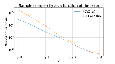
Figure 1: Sample complexities of MDVI with $\alpha=1$ and Q-LEARNING (synchronous version of Q-learning) on Garnets. MDVI is run in the stationary policy setting. Both algorithms use $M=1$. As noted in Section 5, MDVI with $\alpha=1$ is also nearly minimax-optimal.

We compare MDVI to a synchronous version of Q-learning (e.g., Even-Dar et al. (2003)) in a simple setting on a class of random MDPs called Garnets (Archibald et al., 1995), with $\gamma=0.9$. Figure 1 shows the sample complexity of MDVI as a function of $\varepsilon$. We run MDVI on 100 random MDPs, and, given $\varepsilon$, we report the number of samples $KM$ MDVI uses to find $\varepsilon$-optimal policy. We compare this empirical sample complexity with the one of Q-LEARNING, which has a tight quadratic dependency to the horizon (Li et al., 2021a) – compared to the cubic one of MDVI (Theorem 2). Figure 1 shows the difference in sample complexity between the two methods: especially for low $\varepsilon$, MDVI reaches an $\varepsilon$-optimal policy with much fewer samples, up to $H=10$ times less samples for $\varepsilon=10^{-3}$. Complete details, pseudocodes, and results with other $\alpha$ are provided in Appendix H.

7 Conclusion

In this work, we considered and analyzed the sample complexity of a model-free algorithm called MDVI (Geist et al., 2019; Vieillard et al., 2020a) under the generative model setting. We showed that it is nearly minimax-optimal for finding an $\varepsilon$-optimal policy despite its simplicity compared to previous model-free algorithms (Sidford et al., 2018; Wainwright, 2019; Khamaru et al., 2021). We believe that our results are significant for the following three reasons.

First, we demonstrate the effectiveness of KL and entropy regularization. Second, as discussed by Vieillard et al. (2020a), MDVI encompasses various algorithms as special cases or equivalent forms, and our results provide theoretical guarantees for most of them at once. Third, MDVI uses no variance-reduction technique, which leads to multi-epoch algorithms and involved analyses (Sidford et al., 2018; Wainwright, 2019; Khamaru et al., 2021). As such, our analysis is straightforward, and it would be easy to extend it to more complex settings.

A disadvantage of MDVI is that its range of valid $\varepsilon$ is limited compared to previous algorithms (Sidford et al., 2018; Agarwal et al., 2020; Li et al., 2020). It is unclear if this is an artifact of our analysis or the real limitation of MDVI-type algorithms. We leave this topic as a future work.

Appendix

Appendix A Notations

Table 1: Table of Notations

Notation	Meaning
$\mathbf{A}$	action space of size $A$
$H$	effective horizon $H\vcentcolon\nolinebreak\mkern-1.2mu=1/(1-\gamma)$
$P$	transition matrix
$\mathbf{X}$	state space of size $X$
$r$	reward vector bounded by $1$
$\gamma$	discount factor in $[0,1)$
$\varepsilon$	admissible suboptimality
$\delta$	admissible failure probability
$E_{k}$	$E_{k}:(x,a)\mapsto\sum_{j=1}^{k}\alpha^{k-j}\varepsilon_{j}(x,a)$
$\varepsilon_{k}$	$\varepsilon_{k}:(x,a)\mapsto\gamma\widehat{P}_{k-1}v_{k-1}(x,a)-\gamma Pv_{k-1}(x,a)$
$A_{k},A_{\infty},A_{\gamma,k}$	$\sum_{j=0}^{k-1}\alpha^{j}$, $\sum_{j=0}^{\infty}\alpha^{j}$, $\sum_{j=0}^{k-1}\alpha^{j}\gamma^{k-j}$
E1	event of small $E_{k}$ for all $k$ (not variance-aware)
E2	event of small $\varepsilon_{k}$ for all $k$ (not variance-aware)
E3	event of small $E_{k}$ for all $k$ (variance-aware)
E4	event of small $\varepsilon_{k}$ for all $k$ (variance-aware)
$\mathbf{F}_{k,m}$	$\sigma$-algebra in the filtration (cf. Section 5)
$K$	number of value updates
$M$	number of samples per each value update
$P^{\pi}$	$P^{\pi}\vcentcolon\nolinebreak\mkern-1.2mu=P\pi$
$P^{i}_{j}$, $P_{*}^{i}$	$P^{i}_{j}\vcentcolon\nolinebreak\mkern-1.2mu=P^{\pi_{i}}P^{\pi_{i-1}}\cdots P^{\pi_{j+1}}P^{\pi_{j}}$, $P_{*}^{i}\vcentcolon\nolinebreak\mkern-1.2mu=(P^{\pi_{*}})^{i}$
$T^{\pi}$, $T^{i}_{j}$	Bellman operator for a policy $\pi$, $T^{i}_{j}\vcentcolon\nolinebreak\mkern-1.2mu=T^{\pi_{i}}T^{\pi_{i-1}}\cdots T^{\pi_{j+1}}T^{\pi_{j}}$
$V_{k}$	an upper bound for $E_{k}$’s predictive quadratic variance (cf. Lemma 7)
$W_{k}$	an upper bound for $\varepsilon_{k}$’s predictive quadratic variance (cf. Lemma 8)
$s_{k}$	$s_{k}\vcentcolon\nolinebreak\mkern-1.2mu=q_{k}+\alpha s_{k-1}$ (cf. MDVI)
$v_{k}$	$v_{k}\vcentcolon\nolinebreak\mkern-1.2mu=w_{k}-\alpha w_{k-1}$ (cf. MDVI)
$w_{k}$	$w_{k}(x)\vcentcolon\nolinebreak\mkern-1.2mu=\max_{a\in\mathbf{A}}s_{k}(x,a)$ (cf. MDVI)
$\alpha$	$\alpha\vcentcolon\nolinebreak\mkern-1.2mu=\tau/(\tau+\kappa)$, weight for $s_{k}$ updates (cf. MDVI and Appendix B)
$\beta$	$\beta\vcentcolon\nolinebreak\mkern-1.2mu=1/(\tau+\kappa)$, inverse temperature for $\pi_{k}$ (cf. Section 4 and Appendix B)
$\iota_{1}$, $\iota_{2}$	$\iota_{1}\vcentcolon\nolinebreak\mkern-1.2mu=\log(8KXA/\delta)$, $\iota_{2}\vcentcolon\nolinebreak\mkern-1.2mu=\log(16KXA/\delta)$
$\pi_{k}^{\prime}$	a non-stationary policy that follows $\pi_{k},\pi_{k-1},\ldots$ sequentially (cf. Section 5)
$\square$	an indefinite constant independent of $H$, $X$, $A$, $\varepsilon$, and $\delta$

Appendix B Equivalence of MDVI Update Rules

We show the equivalence of MDVI’s updates (1) and (2) to those used in MDVI. We first recall MDVI’s updates (1) and (2):

$$q_{k+1}=r+\gamma P^{\pi_{k}}\left\lparen q_{k}-\tau\log\frac{\pi_{k}}{\pi_{k-1}}-\kappa\log\pi_{k}\right\rparen+\varepsilon_{k}\,,$$ (40)

$$\text{where }\pi_{k}\left\lparen\cdot\middle|x\right\rparen=\operatorname*{arg\,max}_{p\in\Delta(\mathbf{A})}\sum_{a\in\mathbf{A}}p(a)\left\lparen q_{k}(s,a)-\tau\log\frac{p(a)}{\pi_{k-1}\left\lparen a\middle|x\right\rparen}-\kappa\log p(a)\right\rparen\text{ for all }x\in\mathbf{X}\,,$$ (41)

The policy update (2) can be rewritten as follows (e.g., Equation (5) of Kozuno et al. (2019)):

$$\pi_{k}(a|x)=\frac{\pi_{k-1}(a|x)^{\alpha}\exp\left\lparen\beta q_{k}(x,a)\right\rparen}{\sum_{b\in\mathbf{A}}\pi_{k-1}(b|x)^{\alpha}\exp\left\lparen\beta q_{k}(x,b)\right\rparen}\,,$$ (42)

where $\alpha\vcentcolon\nolinebreak\mkern-1.2mu=\tau/(\tau+\kappa)$, and $\beta\vcentcolon\nolinebreak\mkern-1.2mu=1/(\tau+\kappa)$. It can be further rewritten as, defining $s_{k}=q_{k}+\alpha s_{k-1}$

$$\pi_{k}(a|x)=\frac{\exp\left\lparen\beta s_{k}(x,a)\right\rparen}{\sum_{b\in\mathbf{A}}\exp\left\lparen\beta s_{k}(x,b)\right\rparen}\,.$$ (43)

Plugging in this policy expression to $v_{k}$, we deduce that

$$v_{k}(x) =\frac{1}{\beta}\log\sum_{a\in\mathbf{A}}\exp\left\lparen\beta q_{k}(x,a)+\alpha\log\pi_{k-1}(a|x)\right\rparen$$ (44)

$$=\frac{1}{\beta}\log\sum_{a\in\mathbf{A}}\exp\left\lparen\beta s_{k}(x,a)\right\rparen-\frac{\alpha}{\beta}\log\sum_{a\in\mathbf{A}}\exp\left\lparen\beta s_{k-1}(x,a)\right\rparen\,.$$ (45)

Kozuno et al. (2019, Appendix B) show that when $\beta\to\infty$, $v_{k}(x)=w_{k}(x)-\alpha w_{k-1}(x)\,.$ Furthermore, the Boltzmann policy becomes a greedy policy. Accordingly, the update rules used in MDVI is a limit case of the original MDVI updates.

Appendix C Auxiliary Lemmas

In this appendix, we prove some auxiliary lemmas used in the proof.

Lemma 11.

For any positive real values $a$ and $b$, $\sqrt{a+b}\leq\sqrt{a}+\sqrt{b}$.

Proof.

Indeed, $a+b\leq a+2\sqrt{ab}+b=(\sqrt{a}+\sqrt{b})^{2}$. ∎

Lemma 12.

For any real values $(a_{n})_{n=1}^{N}$, $(\sum_{n=1}^{N}a_{n})^{2}\leq N\sum_{n=1}^{N}a_{n}^{2}$.

Proof.

Indeed, from the Cauchy–Schwarz inequality,

$$\left\lparen\sum_{n=1}^{N}a_{n}\cdot 1\right\rparen^{2}\leq\left\lparen\sum_{n=1}^{N}1\right\rparen\left\lparen\sum_{n=1}^{N}a_{n}^{2}\right\rparen=N\sum_{n=1}^{N}a_{n}^{2}\,,$$ (46)

which is the desired result. ∎

Lemma 13.

For any $k\in[K]$,

$$A_{\gamma,k}=\begin{cases}\gamma\dfrac{\alpha^{k}-\gamma^{k}}{\alpha-\gamma}&\text{if }\alpha\neq\gamma\\ k\gamma^{k}&\text{otherwise}\end{cases}\,.$$ (47)

Proof.

Indeed, if $\alpha\neq\gamma$

$$A_{\gamma,k}=\sum_{j=0}^{k-1}\alpha^{j}\gamma^{k-j}=\gamma^{k}\frac{(\alpha/\gamma)^{k}-1}{(\alpha/\gamma)-1}=\gamma\frac{\alpha^{k}-\gamma^{k}}{\alpha-\gamma}\,.$$ (48)

If $\alpha=\gamma$, $A_{\gamma,k}=k\gamma^{k}$ by definition. ∎

Lemma 14.

For any real value $x\in(0,1]$, $1-x\leq\log(1/x)$.

Proof.

Since $\log(1/x)$ is convex and differentiable, $\log(1/x)\geq\log(1/y)-(x-y)/y$. Choosing $y=1$, we concludes the proof. ∎

Lemma 15.

Suppose $\alpha,\gamma\in[0,1)$, $\varepsilon\in(0,1]$, $c\in[1,\infty)$, $m\in\mathbf{N}$, and $n\in[0,\infty)$. Let $K\vcentcolon\nolinebreak\mkern-1.2mu=\dfrac{m}{1-\alpha}\log\dfrac{cH}{\varepsilon}$. Then,

$$K^{n}\alpha^{K}\leq\left\lparen\frac{mn}{(1-\alpha)e}\right\rparen^{n}\left\lparen\dfrac{\varepsilon}{cH}\right\rparen^{m-1}\,.$$ (49)

Proof.

Using Lemma 14,

$$K=\frac{m}{1-\alpha}\log\dfrac{cH}{\varepsilon}\geq\log_{\alpha}\left\lparen\dfrac{\varepsilon}{cH}\right\rparen^{m}.$$ (50)

Therefore,

$$K^{n}\alpha^{K}\leq\left\lparen\frac{m}{1-\alpha}\log\dfrac{cH}{\varepsilon}\right\rparen^{n}\left\lparen\dfrac{\varepsilon}{cH}\right\rparen^{m}=\frac{m^{n}}{(1-\alpha)^{n}}\left\lparen\dfrac{\varepsilon}{cH}\right\rparen^{m}\left\lparen\log\dfrac{cH}{\varepsilon}\right\rparen^{n}\,.$$ (51)

Since $x\left\lparen\log\dfrac{1}{x}\right\rparen^{n}\leq\left\lparen\dfrac{n}{e}\right\rparen^{n}$ for any $x\in(0,1]$ as shown later,

$$K^{n}\alpha^{K}\leq\left\lparen\frac{mn}{(1-\alpha)e}\right\rparen^{n}\left\lparen\dfrac{\varepsilon}{cH}\right\rparen^{m-1}\,.$$ (52)

Now it remains to show $f(x)\vcentcolon\nolinebreak\mkern-1.2mu=x\left\lparen\log\dfrac{1}{x}\right\rparen^{n}\leq\left\lparen\dfrac{n}{e}\right\rparen^{n}$ for $x<1$. We have that

$$f^{\prime}(x)=(-\log x)^{n}-n(-\log x)^{n-1}\implies f^{\prime}(x)=0\text{ at }x=e^{-n}.$$ (53)

Therefore, $f$ takes its maximum $\left\lparen\dfrac{n}{e}\right\rparen^{n}$ at $e^{-n}$ when $x\in(0,1)$. ∎

The following lemma is a special case of a well-known inequality that for any increasing function $f$

$$\sum_{k=1}^{K}f(k)\leq\int_{1}^{K+1}f(x)dx\,.$$ (54)

Lemma 16.

For any $K\in\mathbf{N}$ and $n\in[0,\infty)$, $\displaystyle\sum_{k=1}^{K}k^{n}\leq\frac{1}{n+1}(K+1)^{n+1}$.

Appendix D Tools from Probability Theory

We extensively use the following two concentration inequalities. The first one is Azuma-Hoeffding inequality (Azuma, 1967; Hoeffding, 1963; Boucheron et al., 2013), and the second one is Bernstein’s inequality (Bernstein, 1946; Boucheron et al., 2013) for a martingale (Lattimore & Szepesvari, 2020, Excercises 5.14 (f)). For a real-valued stochastic process $(X_{n})_{n=1}^{N}$ adapted to a filtration $(\mathcal{F}_{n})_{n=1}^{N}$, we let $\mathbb{E}_{n}[X_{n}]\vcentcolon\nolinebreak\mkern-1.2mu=\mathbb{E}\mathopen{[}X_{n}\mathord{|}\mathcal{F}_{n-1}\mathclose{]}$ for $n\geq 1$, and $\mathbb{E}_{1}[X_{1}]\vcentcolon\nolinebreak\mkern-1.2mu=\mathbb{E}\mathopen{[}X_{1}\mathclose{]}$.

Lemma 17 (Azuma-Hoeffding Inequality).

Consider a real-valued stochastic process $(X_{n})_{n=1}^{N}$ adapted to a filtration $(\mathcal{F}_{n})_{n=1}^{N}$. Assume that $X_{n}\in[l_{n},u_{n}]$ and $\mathbb{E}_{n}[X_{n}]=0$ almost surely, for all $n$. Then,

$$\mathbb{P}\left\lparen\sum_{n=1}^{N}X_{n}\geq\sqrt{\sum_{n=1}^{N}\frac{(u_{n}-l_{n})^{2}}{2}\log\frac{1}{\delta}}\right\rparen\leq\delta$$ (55)

for any $\delta\in(0,1)$.

Lemma 18 (Bernstein’s Inequality).

Consider a real-valued stochastic process $(X_{n})_{n=1}^{N}$ adapted to a filtration $(\mathcal{F}_{n})_{n=1}^{N}$. Suppose that $X_{n}\leq U$ and $\mathbb{E}_{n}[X_{n}]=0$ almost surely, for all $n$. Then, letting $V^{\prime}\vcentcolon\nolinebreak\mkern-1.2mu=\sum_{n=1}^{N}\mathbb{E}_{n}[X_{n}^{2}]$,

$$\mathbb{P}\left\lparen\sum_{n=1}^{N}X_{n}\geq\frac{2U}{3}\log\frac{1}{\delta}+\sqrt{2V\log\frac{1}{\delta}}\text{ and }V^{\prime}\leq V\right\rparen\leq\delta$$ (56)

for any $V\in[0,\infty)$ and $\delta\in(0,1)$.

In our analysis, we use the following corollary of this Bernstein’s inequality.

Lemma 19 (Conditional Bernstein’s Inequality).

Consider the same notations and assumptions in Lemma 18. Furthermore, let $\mathcal{E}$ be an event that implies $V^{\prime}\leq V$ for some $V\in[0,\infty)$ with $\mathbb{P}(\mathcal{E})\geq 1-\delta^{\prime}$ for some $\delta^{\prime}\in(0,1)$. Then,

$$\mathbb{P}\left\lparen\sum_{n=1}^{N}X_{n}\geq\frac{2U}{3}\log\frac{1}{\delta(1-\delta^{\prime})}+\sqrt{2V\log\frac{1}{\delta(1-\delta^{\prime})}}\middle|\mathcal{E}\right\rparen\leq\delta$$ (57)

for any $\delta\in(0,1)$.

Proof.

Let $A$ and $B$ denote the events of

$$\sum_{n=1}^{N}X_{n}\geq\frac{2U}{3}\log\frac{1}{\delta(1-\delta^{\prime})}+\sqrt{2V\log\frac{1}{\delta(1-\delta^{\prime})}}$$ (58)

and $V^{\prime}\leq V$, respectively. Since $\mathcal{E}\subset B$, it follows that $A\cap\mathcal{E}\subset A\cap B$, and $\mathbb{P}(A\cap\mathcal{E})\leq\mathbb{P}(A\cap B)$. Accordingly,

$$\mathbb{P}(A|\mathcal{E})=\frac{\mathbb{P}(A\cap\mathcal{E})}{\mathbb{P}(\mathcal{E})}\leq\frac{\mathbb{P}(A\cap B)}{\mathbb{P}(\mathcal{E})}\stackrel{{\scriptstyle\scriptscriptstyle(\mkern-1.5mua\mkern-1.5mu)}}{{\leq}}\frac{\delta(1-\delta^{\prime})}{\mathbb{P}(\mathcal{E})}\stackrel{{\scriptstyle\scriptscriptstyle(\mkern-1.5mub\mkern-1.5mu)}}{{\leq}}\delta\,,$$ (59)

where (a) follows from Lemma 18, and (b) follows from $\mathbb{P}(\mathcal{E})\geq 1-\delta^{\prime}$. ∎

Lemma 20 (Popoviciu’s Inequality for Variances).

The variance of any random variable bounded by $x$ is bounded by $x^{2}$.

Appendix E Total Variance Technique

The following lemma is due to Azar et al. (2013).

Lemma 21.

Suppose two real-valued random variables $X,Y$ whose variances, $\mathbb{V}X$ and $\mathbb{V}Y$, exist and are finite. Then, $\sqrt{\mathbb{V}X}\leq\sqrt{\mathbb{V}\left[X-Y\right]}+\sqrt{\mathbb{V}Y}$.

For completeness, we prove Lemma 21.

Proof.

Indeed, from Cauchy-Schwartz inequality,

$$\mathbb{V}X =\mathbb{V}\mathopen{[}X-Y+Y\mathclose{]}$$ (60)

$$=\mathbb{V}\mathopen{[}X-Y\mathclose{]}+\mathbb{V}Y+2\mathbb{E}\left[(X-Y-\mathbb{E}\mathopen{[}X-Y\mathclose{]})(Y-\mathbb{E}Y)\right]$$ (61)

$$\leq\mathbb{V}\mathopen{[}X-Y\mathclose{]}+\mathbb{V}Y+2\sqrt{\mathbb{V}\mathopen{[}X-Y\mathclose{]}\mathbb{V}Y}=\left\lparen\sqrt{\mathbb{V}\left[X-Y\right]}+\sqrt{\mathbb{V}Y}\right\rparen^{2}\,.$$ (62)

This is the desired result. ∎

The following lemma is an extension of Lemma 7 by Azar et al. (2013) and its refined version by Agarwal et al. (2020).

Lemma 22.

Suppose a sequence of deterministic policies $(\pi_{k})_{k=0}^{K}$ and let

$$q^{\pi^{\prime}_{k}}\vcentcolon\nolinebreak\mkern-1.2mu=\begin{cases}r+\gamma Pv^{\pi^{\prime}_{k-1}}&\text{for }k\in[K]\\ q^{\pi_{0}}&\text{for }k=0\end{cases}\,.$$ (63)

Furthermore, let $\sigma_{k}^{2}$ and $\Sigma_{k}^{2}$ be non-negative functions over $\mathbf{X}\times\mathbf{A}$ defined by

$$\sigma_{k}^{2}(x,a)\vcentcolon\nolinebreak\mkern-1.2mu=\begin{cases}P\mathopen{\lparen}v^{\pi^{\prime}_{k-1}}\mathclose{\rparen}^{2}(x,a)-\mathopen{\lparen}Pv^{\pi^{\prime}_{k-1}}\mathclose{\rparen}^{2}(x,a)&\text{for }k\in[K]\\ P\mathopen{\lparen}v^{\pi_{0}}\mathclose{\rparen}^{2}(x,a)-\mathopen{\lparen}Pv^{\pi_{0}}\mathclose{\rparen}^{2}(x,a)&\text{for }k=0\end{cases}$$ (64)

and

$$\Sigma_{k}^{2}(x,a)\vcentcolon\nolinebreak\mkern-1.2mu=\mathbb{E}_{k}\left[\left\lparen\sum_{t=0}^{\infty}\gamma^{t}r(X_{t},A_{t})-q^{\pi^{\prime}_{k}}(X_{0},A_{0})\right\rparen^{2}\middle|X_{0}=x,A_{0}=a\right]$$ (65)

for $k\in\{0\}\cup[K]$, where $\mathbb{E}_{k}$ is the expectation over $(X_{t},A_{t})_{t=0}^{\infty}$ wherein $A_{t}\sim\pi_{k-t}(\cdot|X_{t})$ until $t=k$, and $A_{t}\sim\pi_{0}(\cdot|X_{t})$ thereafter. Then,

$$\sum_{j=0}^{k-1}\gamma^{j+1}P_{k-j}^{k-1}\sigma_{k-j}\leq\sqrt{2H^{3}}$$ (66)

for any $k\in[K]$.

For its proof, we need the following lemma.

Lemma 23.

Suppose a sequence of deterministic policies $(\pi_{k})_{k=0}^{K}$ and notations in Lemma 22. Then, for any $k\in[K]$, we have that

$$\Sigma_{k}^{2}=\gamma^{2}\sigma_{k}^{2}+\gamma^{2}P^{\pi_{k-1}}\Sigma_{k-1}^{2}\,.$$ (67)

Proof.

Let $R_{s}^{u}\vcentcolon\nolinebreak\mkern-1.2mu=\sum_{t=s}^{u}\gamma^{t-s}r(X_{t},A_{t})$ and $\mathbb{E}_{k}\left[\cdot\middle|x,a\right]\vcentcolon\nolinebreak\mkern-1.2mu=\mathbb{E}_{k}\left[\cdot\middle|X_{0}=x,A_{0}=a\right]$. We have that

$$\Sigma_{k}^{2}(x,a)=\mathbb{E}_{k}\left[\left\lparen R_{0}^{\infty}-q^{\pi^{\prime}_{k}}(X_{0},A_{0})\right\rparen^{2}\middle|x,a\right]\vcentcolon\nolinebreak\mkern-1.2mu=\mathbb{E}_{k}\left[\left\lparen I_{1}+\gamma I_{2}\right\rparen^{2}\middle|x,a\right]\,,$$ (68)

where $I_{1}\vcentcolon\nolinebreak\mkern-1.2mu=r(X_{0},A_{0})+\gamma q^{\pi^{\prime}_{k-1}}(X_{1},A_{1})-q^{\pi^{\prime}_{k}}(X_{0},A_{0})$, and $I_{2}\vcentcolon\nolinebreak\mkern-1.2mu=R_{1}^{\infty}-q^{\pi^{\prime}_{k-1}}(X_{1},A_{1})$. With these notations, we see that

$$\Sigma_{k}^{2}(x,a) =\mathbb{E}_{k}\mathopen{\bigl{[}}I_{1}^{2}+\gamma^{2}I_{2}^{2}+2\gamma I_{1}I_{2}\mathord{\bigm{|}}x,a\mathclose{\bigr{]}}$$ (69)

$$=\mathbb{E}_{k}\mathopen{\bigl{[}}I_{1}^{2}+\gamma^{2}I_{2}^{2}+2\gamma I_{1}\mathbb{E}_{k-1}\left[I_{2}\middle|X_{1},A_{1}\right]\mathord{\bigm{|}}x,a\mathclose{\bigr{]}}$$ (70)

$$=\mathbb{E}_{k}\mathopen{\bigl{[}}I_{1}^{2}\mathord{\bigm{|}}x,a\mathclose{\bigr{]}}+\gamma^{2}\mathbb{E}_{k}\mathopen{\bigl{[}}I_{2}^{2}\mathord{\bigm{|}}x,a\mathclose{\bigr{]}}$$ (71)

$$=\mathbb{E}_{k}\mathopen{\bigl{[}}I_{1}^{2}\mathord{\bigm{|}}x,a\mathclose{\bigr{]}}+\gamma^{2}P^{\pi_{k-1}}\Sigma_{k-1}^{2}(x,a)\,,$$ (72)

where the second line follows from the law of total expectation, and the third line follows since $\mathbb{E}_{k-1}\left[I_{2}\middle|X_{1},A_{1}\right]=0$ due to the Markov property. The first term in the last line is $\gamma^{2}\sigma_{k}^{2}(x,a)$ because

$$\mathbb{E}_{k}\mathopen{\bigl{[}}I_{1}^{2}\mathord{\bigm{|}}x,a\mathclose{\bigr{]}} \stackrel{{\scriptstyle\scriptscriptstyle(\mkern-1.5mua\mkern-1.5mu)}}{{=}}\gamma^{2}\mathbb{E}_{k}\mathopen{\Biggl{[}}\mathopen{\Bigl{\lparen}}\underbrace{q^{\pi_{k-1}^{\prime}}(X_{1},A_{1})}_{v^{\pi_{k-1}^{\prime}}(X_{1})\text{ from (b)}}-(Pv^{\pi_{k-1}^{\prime}})(X_{0},A_{0})\mathclose{\Bigr{\rparen}}^{2}\mathord{\Biggm{|}}x,a\mathclose{\Biggr{]}}$$ (73)

$$=\gamma^{2}\left\lparen P\left\lparen v^{\pi_{k-1}^{\prime}}\right\rparen^{2}\right\rparen(x,a)+\gamma^{2}(Pv^{\pi_{k-1}^{\prime}})^{2}(x,a)-2(Pv^{\pi_{k-1}^{\prime}})^{2}(x,a)$$ (74)

$$=\gamma^{2}\left\lparen P\left\lparen v^{\pi_{k-1}^{\prime}}\right\rparen^{2}\right\rparen(x,a)-\gamma^{2}(Pv^{\pi_{k-1}^{\prime}})^{2}(x,a)\,,$$ (75)

where (a) follows from the definition that $q^{\pi_{k}^{\prime}}=r+\gamma Pv^{\pi^{\prime}_{k-1}}$, and (b) follows since the policies are deterministic. From this argument, it is clear that $\Sigma_{k}^{2}=\gamma^{2}\sigma_{k}^{2}+\gamma^{2}P^{\pi_{k-1}}\Sigma_{k-1}^{2}\,,$ which is the desired result. ∎

Now, we are ready to prove Lemma 22.

Proof of Lemma 22.

Let $H_{k}\vcentcolon\nolinebreak\mkern-1.2mu=\sum_{j=0}^{k-1}\gamma^{j}$. Using Jensen’s inequality twice,

$$\sum_{j=0}^{k-1}\gamma^{j+1}P_{k-j}^{k-1}\sigma_{k-j} \leq\sum_{j=0}^{k-1}{\gamma^{j+1}\sqrt{P_{k-j}^{k-1}\sigma_{k-j}^{2}}}$$ (76)

$$\leq\gamma H_{k}\sum_{j=0}^{k-1}{\frac{\gamma^{j+1}}{H_{k}}\sqrt{P_{k-j}^{k-1}\sigma_{k-j}^{2}}}$$ (77)

$$\leq\sqrt{H_{k}\sum_{j=0}^{k-1}{\gamma^{j+2}P_{k-j}^{k-1}\sigma_{k-j}^{2}}}\leq\sqrt{H\sum_{j=0}^{k-1}{\gamma^{j+2}P_{k-j}^{k-1}\sigma_{k-j}^{2}}}\,.$$ (78)

From Lemma 23, we have that

$$\sum_{j=0}^{k-1}{\gamma^{j+2}P_{k-j}^{k-1}\sigma_{k-j}^{2}}$$ (79)

$$=\sum_{j=0}^{k-1}{\gamma^{j}P_{k-j}^{k-1}\left\lparen\Sigma_{k-j}^{2}-\gamma^{2}P^{\pi_{k-1-j}}\Sigma_{k-1-j}^{2}\right\rparen}$$ (80)

$$=\sum_{j=0}^{k-1}{\gamma^{j}P_{k-j}^{k-1}\left\lparen\Sigma_{k-j}^{2}-\gamma P^{\pi_{k-1-j}}\Sigma_{k-1-j}^{2}+\gamma(1-\gamma)P^{\pi_{k-1-j}}\Sigma_{k-1-j}^{2}\right\rparen}$$ (81)

$$=\sum_{j=0}^{k-1}\gamma^{j}P_{k-j}^{k-1}\Sigma_{k-j}^{2}-\sum_{j=1}^{k}\gamma^{j}P_{k-j}^{k-1}\Sigma_{k-j}^{2}+\gamma(1-\gamma)\sum_{j=0}^{k-1}\gamma^{j}P_{k-1-j}^{k-1}\Sigma_{k-1-j}^{2}\,.$$ (82)

The final line is equal to $\Sigma_{k}^{2}-\gamma^{k}P_{0}^{k-1}\Sigma_{0}^{2}+\gamma(1-\gamma)\sum_{j=0}^{k-1}\gamma^{j}P_{k-1-j}^{k-1}\Sigma_{k-1-j}^{2}$. Finally, from the monotonicity of stochastic matrices and that $\mathbf{0}\leq\Sigma_{j}^{2}\leq H^{2}\mathbf{1}$ for any $j$,

$$\sum_{j=0}^{k-1}\gamma^{j+1}P_{k-j}^{k-1}\sigma_{k-j}\leq\sqrt{2H^{3}}\,.$$ (83)

This concludes the proof. ∎

Appendix F Proof of Lemmas for Theorem 1 (Bound for a Non-Stationary Policy)

Before starting the proof, we introduce some notations and facts frequently used in the proof.

Frequently Used Facts.

We frequently use the following fact, which follows from definitions:

$$s_{k}=A_{k}r+\gamma Pw_{k-1}+E_{k}\quad\text{for any }k\in[K]\,.$$ (84)

Indeed, $s_{k}=\sum_{j=1}^{k}\alpha^{k-j}(r+\gamma P(w_{j-1}-\alpha w_{j-2})+\varepsilon_{j})=A_{k}r+\gamma Pw_{k-1}+E_{k}$. In addition, we often mention the “monotonicity” of stochastic matrices: any stochastic matrix $\rho$ satisfies that $\rho v\geq\rho u$ for any vectors $v,u$ such that $v\geq u$. Examples of stochastic matrices in the proof are $P$, $\pi$, $P^{\pi}$, and $\pi P$. The monotonicity property is so frequently used that we do not always mention it.

F.1 Proof of Lemma 1 (Error Propagation Analysis)

Proof.

Note that

$$\mathbf{0}\leq v^{*}-v^{\pi^{\prime}_{k}}=\frac{A_{k}}{A_{\infty}}\left\lparen v^{*}-v^{\pi^{\prime}_{k}}\right\rparen+\alpha^{k}\left\lparen v^{*}-v^{\pi^{\prime}_{k}}\right\rparen\leq\frac{A_{k}}{A_{\infty}}\left\lparen v^{*}-v^{\pi^{\prime}_{k}}\right\rparen+2H\alpha^{k}\mathbf{1}$$ (85)

since $v^{*}-v^{\pi^{\prime}_{k}}\leq 2H\mathbf{1}$. Therefore, we need an upper bound for $A_{k}(v^{*}-v^{\pi^{\prime}_{k}})$. We decompose $A_{k}(v^{*}-v^{\pi^{\prime}_{k}})$ to $A_{k}v^{*}-w_{k}$ and $w_{k}-A_{k}v^{\pi^{\prime}_{k}}$. Then, we derive upper bounds for each of them (inequalities (86) and (91), respectively). The desired result is obtained by summing up those bounds.

Upper bound for $A_{k}v^{*}-w_{k}$.

We prove by induction that for any $k\in[K]$,

$$A_{k}v^{*}-w_{k}\leq HA_{\gamma,k}\mathbf{1}-\sum_{j=0}^{k-1}\gamma^{j}\pi_{*}P_{*}^{j}E_{k-j}\,.$$ (86)

We have that

$$A_{k}v^{*}-w_{k} \stackrel{{\scriptstyle\scriptscriptstyle(\mkern-1.5mua\mkern-1.5mu)}}{{\leq}}\pi_{*}(A_{k}q^{*}-s_{k})$$ (87)

$$\stackrel{{\scriptstyle\scriptscriptstyle(\mkern-1.5mub\mkern-1.5mu)}}{{=}}\pi_{*}\left\lparen A_{k}q^{*}-A_{k}r-\gamma Pw_{k-1}-E_{k}\right\rparen$$ (88)

$$\stackrel{{\scriptstyle\scriptscriptstyle(\mkern-1.5muc\mkern-1.5mu)}}{{=}}\pi_{*}\left\lparen\gamma P(A_{k}v^{*}-w_{k-1})-E_{k}\right\rparen$$ (89)

$$\stackrel{{\scriptstyle\scriptscriptstyle(\mkern-1.5mud\mkern-1.5mu)}}{{\leq}}\pi_{*}\left\lparen\gamma P(A_{k-1}v^{*}-w_{k-1})+\alpha^{k-1}\gamma H\mathbf{1}-E_{k}\right\rparen\,,$$ (90)

where (a) is due to the greediness of $\pi_{k}$, (b) is due to the equation (84), (c) is due to the Bellman equation for $q^{*}$, and (d) is due to the fact that $(A_{k}-A_{k-1})v^{*}=\alpha^{k-1}v^{*}\leq\alpha^{k-1}H\mathbf{1}$. From this result and the fact that $w_{0}=\mathbf{0}$, $A_{1}v^{*}-w_{1}\leq\gamma H\mathbf{1}-\pi_{*}E_{1}\,.$ Therefore, the inequality (86) holds for $k=1$. From the step (d) above and induction, it is straightforward to verify that the inequality (86) holds for other $k$.

Upper bound for $w_{k}-A_{k}v^{\pi^{\prime}_{k}}$.

We prove by induction that for any $k\in[K]$,

$$w_{k}-A_{k}v^{\pi^{\prime}_{k}}\leq HA_{\gamma,k}\mathbf{1}+\sum_{j=0}^{k-1}\gamma^{j}\pi_{k}P_{k-j}^{k-1}E_{k-j}\,.$$ (91)

Recalling that $v^{\pi^{\prime}_{k}}=\pi_{k}T_{0}^{k-1}q^{\pi_{0}}$, we deduce that

$$w_{k}-A_{k}v^{\pi^{\prime}_{k}} \stackrel{{\scriptstyle\scriptscriptstyle(\mkern-1.5mua\mkern-1.5mu)}}{{=}}\pi_{k}\left\lparen s_{k}-A_{k}T_{0}^{k-1}q^{\pi_{0}}\right\rparen$$ (92)

$$\stackrel{{\scriptstyle\scriptscriptstyle(\mkern-1.5mub\mkern-1.5mu)}}{{=}}\pi_{k}\left\lparen A_{k}r+\gamma Pw_{k-1}-A_{k}T_{1}^{k-1}q^{\pi_{0}}+E_{k}\right\rparen$$ (93)

$$\stackrel{{\scriptstyle\scriptscriptstyle(\mkern-1.5muc\mkern-1.5mu)}}{{=}}\pi_{k}\left\lparen\gamma P\left\lparen w_{k-1}-A_{k}v^{\pi^{\prime}_{k-1}}\right\rparen+E_{k}\right\rparen$$ (94)

$$\stackrel{{\scriptstyle\scriptscriptstyle(\mkern-1.5mud\mkern-1.5mu)}}{{\leq}}\pi_{k}\left\lparen\gamma P(w_{k-1}-A_{k-1}v^{\pi^{\prime}_{k-1}})+\alpha^{k-1}\gamma H\mathbf{1}+E_{k}\right\rparen\,,$$ (95)

where (a) follows from the definition of $w_{k}$, (b) is due to the equation (84), (c) follows from the definition of the Bellman operator, and (d) is due to the fact that $(A_{k}-A_{k-1})v^{\pi^{\prime}_{k-1}}=\alpha^{k-1}v^{\pi^{\prime}_{k-1}}\geq-\alpha^{k-1}H\mathbf{1}$. From this result and the fact that $w_{0}=\mathbf{0}$,

$$w_{1}-A_{1}v^{\pi^{\prime}_{1}}\leq\pi_{1}\left\lparen\gamma Pw_{0}+\gamma H\mathbf{1}+E_{1}\right\rparen\leq\gamma H\mathbf{1}+\pi_{1}E_{1}\,.$$ (96)

Therefore, the inequality (91) holds for $k=1$. From the step (d) above and induction, it is straightforward to verify that the inequality (91) holds for other $k$. ∎

F.2 Proof of Lemmas 2 and 3 (Coarse State-Value Bound)

The next lemma is necessary to bound $E_{k}$ by using the Azuma-Hoeffding inequality (Lemma 17).

Lemma 24.

For any $k\in[K]$, $v_{k-1}$ is bounded by $H$.

Proof.

We prove the claim by induction. The claim holds for $k=1$ since $v_{0}=\mathbf{0}$ by definition. Assume that $v_{k-1}$ is bounded by $H$ for some $k\geq 1$. Then, from the greediness of the policies $\pi_{k}$ and $\pi_{k-1}$,

$$\pi_{k-1}q_{k}=\pi_{k-1}(s_{k}-\alpha s_{k-1})\leq v_{k}\leq\pi_{k}(s_{k}-\alpha s_{k-1})=\pi_{k}q_{k}$$ (97)

Since $q_{k}=r+\gamma\widehat{P}_{k-1}v_{k-1}$ is bounded by $H$ due to the induction hypothesis, the claim holds. ∎

Proof of Lemma 2.

Consider a fixed $k\in[K]$ and $(x,a)\in\mathbf{X}\times\mathbf{A}$. Since

$$E_{k}(x,a)=\frac{\gamma}{M}\sum_{j=1}^{k}\alpha^{k-j}\sum_{m=1}^{M}\underbrace{\left\lparen v_{j-1}(y_{j-1,m,x,a})-Pv_{j-1}(x,a)\right\rparen}_{\text{bounded by }2H\text{ from \lx@cref{creftype~refnum}{lemma:v is bounded}}}\,,$$ (98)

$E_{k}(x,a)$ is a sum of bounded martingale differences with respect to the filtraion $(\mathbf{F}_{j,m})_{j=1,m=1}^{k,M}$. Therefore, using the Azuma-Hoeffding inequality (Lemma 17),

$$\mathbb{P}\left\lparen\mathopen{\lvert}E_{k}\mathclose{\rvert}(x,a)\geq 3H\sqrt{\frac{A_{\infty}\iota_{1}}{M}}\right\rparen\leq\frac{\delta}{4KXA}\,,$$ (99)

where the bound in $\mathbb{P}(\cdot)$ is simplified by $2\sqrt{2}\gamma\leq 3$ and $\sum_{j=1}^{k}\alpha^{2(k-j)}\leq\sum_{j=1}^{k}\alpha^{k-j}=A_{\infty}$. Taking the union bound over $(x,a,k)\in\mathbf{X}\times\mathbf{A}\times[K]$,

$$\mathbb{P}\left\lparen\mathcal{E}_{1}\right\rparen\geq 1-\sum_{(x,a)\in\mathbf{X}\times\mathbf{A}}\sum_{k=1}^{K}\mathbb{P}\left\lparen\mathopen{\lvert}E_{k}\mathclose{\rvert}(x,a)\geq 3H\sqrt{\frac{A_{\infty}\iota_{1}}{M}}\right\rparen\geq 1-\frac{\delta}{4}\,,$$ (100)

and thus $\mathbb{P}\left\lparen\mathcal{E}_{1}^{c}\right\rparen\leq\delta/4$, which is the desired result. ∎

Proof of Lemma 3.

We condition the proof by the event E1. This event occurs with probability at least $1-\delta/4$. Note that under the current setting of $\alpha$, $A_{\infty}=H$. From Lemma 2 and the settings of $\alpha$ and $M$,

$$\sum_{j=0}^{k-1}\gamma^{j}\left\lparen\pi_{k}P_{k-j}^{k-1}-\pi_{*}P_{*}^{j}\right\rparen E_{k-j}\leq 2\sum_{j=0}^{k-1}\gamma^{j}\mathopen{\lVert}E_{k-j}\mathclose{\rVert_{\infty}}\leq\frac{\square H\sqrt{H}\varepsilon}{\sqrt{c_{2}}}\,.$$ (101)

Thus, from Lemma 1, $v^{*}-v^{\pi^{\prime}_{k}}\leq\square\sqrt{H/c_{2}}\varepsilon+2(H+k)\gamma^{k}\mathbf{1}$. Finally, using Lemma 15,

$$2(H+K)\gamma^{K}\leq\frac{\square\varepsilon}{c_{1}},$$ (102)

and thus,

$$\mathopen{\lVert}v^{*}-v^{\pi^{\prime}_{K}}\mathclose{\rVert_{\infty}}\leq\square\varepsilon\sqrt{\frac{H}{c_{2}}}+\frac{\square\varepsilon}{c_{1}}\leq\square\left\lparen\frac{1}{c_{1}}+\frac{1}{\sqrt{c_{2}}}\right\rparen\sqrt{H}\varepsilon\,.$$ (103)

Therefore, for some $c_{1}$ and $c_{2}$, the claim holds. ∎

F.3 Proof of Lemma 4 (Value Estimation Error Bound)

We first prove an intermediate result.

Lemma 25.

For any $k\in[K]$,

$$v^{\pi^{\prime}_{k-1}}+\sum_{j=0}^{k-1}\gamma^{j}\pi_{k-1}P_{k-1-j}^{k-2}\varepsilon_{k-j}-\gamma^{k}H\mathbf{1}\leq v_{k}\leq v^{\pi^{\prime}_{k}}+\sum_{j=0}^{k-1}\gamma^{j}\pi_{k}P_{k-j}^{k-1}\varepsilon_{k-j}+\gamma^{k}H\mathbf{1}\,.$$ (104)

Proof.

From the greediness of $\pi_{k-1}$, $v_{k}=w_{k}-\alpha w_{k-1}\leq\pi_{k}(s_{k}-\alpha s_{k-1})=\pi_{k}(r+\gamma Pv_{k-1}+\varepsilon_{k})$. By induction on $k$, therefore,

$$v_{k}\leq\sum_{j=0}^{k-1}\gamma^{j}\pi_{k}P_{k-j}^{k-1}\left\lparen r+\varepsilon_{k-j}\right\rparen+\underbrace{\gamma^{k}\pi_{k}P_{0}^{k-1}v_{0}}_{=\mathbf{0}}=\sum_{j=0}^{k-1}\gamma^{j}\pi_{k}P_{k-j}^{k-1}\left\lparen r+\varepsilon_{k-j}\right\rparen\,,$$ (105)

Note that

$$T_{0}^{k-1}q^{\pi_{0}}=\sum_{j=0}^{k-1}\gamma^{j}P_{k-j}^{k-1}r+\gamma^{k}\underbrace{P_{0}^{k-1}q^{\pi_{0}}}_{\geq-H\mathbf{1}}\implies\sum_{j=0}^{k-1}\gamma^{j}P_{k-j}^{k-1}r\leq T_{0}^{k-1}q^{\pi_{0}}+\gamma^{k}H\,.$$ (106)

Accordingly, $v_{k}\leq\pi_{k}T_{0}^{k-1}q^{\pi_{0}}+\sum_{j=0}^{k-1}\gamma^{j}\pi_{k}P_{k-j}^{k-1}\varepsilon_{k-j}+\gamma^{k}H\mathbf{1}\,.$

Similarly, from the greediness of $\pi_{k}$, $v_{k}=w_{k}-\alpha w_{k-1}\geq\pi_{k-1}(s_{k}-\alpha s_{k-1})\geq\pi_{k-1}(r+\gamma Pv_{k-1}+\varepsilon_{k})$. By induction on $k$, therefore,

$$v_{k}\geq\sum_{j=0}^{k-1}\gamma^{j}\pi_{k-1}P_{k-1-j}^{k-2}\left\lparen r+\varepsilon_{k-j}\right\rparen+\underbrace{\gamma^{k-1}\pi_{k-1}P_{0}^{k-2}Pv_{0}}_{=\mathbf{0}}\,.$$ (107)

Note that $T_{0}^{k-2}q^{\pi_{0}}=T_{0}^{k-2}(r+\gamma Pv^{\pi_{0}})$, and

$$T_{0}^{k-2}q^{\pi_{0}}=\sum_{j=0}^{k-1}\gamma^{j}P_{k-1-j}^{k-2}r+\gamma^{k}\underbrace{P_{0}^{k-2}Pv^{\pi_{0}}}_{\leq H\mathbf{1}}\implies\sum_{j=0}^{k-1}\gamma^{j}P_{k-1-j}^{k-2}r\geq T_{0}^{k-2}q^{\pi_{0}}-\gamma^{k}H\,.$$ (108)

Accordingly, $v_{k}\geq\pi_{k-1}T_{0}^{k-2}q^{\pi_{0}}+\sum_{j=0}^{k-1}\gamma^{j}\pi_{k-1}P_{k-1-j}^{k-2}\varepsilon_{k-j}-\gamma^{k}H\mathbf{1}\,.$ ∎

Proof of Lemma 4.

From Lemma 25 and $\pi_{k}T^{\pi_{k-1:1}}q^{\pi_{0}}=v^{\pi^{\prime}_{k}}\leq v^{*}$, we have that

$$v^{\pi^{\prime}_{k-1}}+\sum_{j=0}^{k-1}\gamma^{j}\pi_{k-1}P_{k-1-j}^{k-2}\varepsilon_{k-j}-2\gamma^{k}H\mathbf{1}\leq v_{k}\leq v^{*}+\sum_{j=0}^{k-1}\gamma^{j}\pi_{k}P_{k-j}^{k-1}\varepsilon_{k-j}+2\gamma^{k}H\mathbf{1}\,,$$ (109)

where we loosened the bound by multiplying $\gamma^{k}H$ by $2$. By simple algebra, the lower bound for $v^{*}-v_{k}$ is obtained. On the other hand, from Lemma 1,

$$v^{\pi^{\prime}_{k-1}}\geq v^{*}-\frac{1}{A_{\infty}}\sum_{j=0}^{k-2}\gamma^{j}\left\lparen\pi_{k-1}P_{k-1-j}^{k-2}-\pi_{*}P_{*}^{j}\right\rparen E_{k-1-j}-2H\left\lparen\alpha^{k-1}+\frac{A_{\gamma,k-1}}{A_{\infty}}\right\rparen\mathbf{1}$$ (110)

for any $k\in\{2,\ldots,K\}$. Therefore, we have that

$$v^{*}-v_{k} \leq 2H\left\lparen\alpha^{k-1}+\gamma^{k}+\frac{A_{\gamma,k-1}}{A_{\infty}}\right\rparen\mathbf{1}$$ (111)

$$\hskip 20.00003pt+\frac{1}{A_{\infty}}\sum_{j=0}^{k-2}\gamma^{j}\left\lparen\pi_{k-1}P_{k-1-j}^{k-2}-\pi_{*}P_{*}^{j}\right\rparen E_{k-1-j}-\sum_{j=0}^{k-1}\gamma^{j}\pi_{k-1}P_{k-1-j}^{k-2}\varepsilon_{k-j}$$ (112)

for any $k\in\{2,\ldots,K\}$.

Finally, for $k=1$, since $v_{1}=\pi_{1}q_{1}=\pi_{1}r$,

$$-\gamma H\mathbf{1}\leq\pi_{*}\left\lparen q^{*}-r\right\rparen\leq v^{*}-v_{1}\leq\gamma\pi_{*}Pv^{*}\leq\gamma H\mathbf{1}\,.$$ (113)

As $\Gamma_{1}\geq\mathbf{0}$, the claim holds for $k=1$ too. ∎

F.4 Proof of Lemmas 6 and 5 (Value Estimation Variance Bound)

Proof of Lemma 5.

Consider a fixed $k\in[K]$ and $(x,a)\in\mathbf{X}\times\mathbf{A}$. Since

$$\varepsilon_{k}(x,a)=\frac{\gamma}{M}\sum_{m=1}^{M}\underbrace{\left\lparen v_{k-1}(y_{k-1,m,x,a})-Pv_{k-1}(x,a)\right\rparen}_{\text{bounded by }2H\text{ from \lx@cref{creftype~refnum}{lemma:v is bounded}}}\,,$$ (114)

$\varepsilon_{k}(x,a)$ is a sum of martingale differences with respect to the filtraion $(\mathbf{F}_{k,m})_{m=1}^{M}$ and bounded by $2\gamma H/M$. Therefore, using the Azuma-Hoeffding inequality (Lemma 17),

$$\mathbb{P}\left\lparen\mathopen{\lvert}\varepsilon_{k}\mathclose{\rvert}(x,a)\geq 3H\sqrt{\frac{\iota_{1}}{M}}\right\rparen\leq\frac{\delta}{4KXA}\,,$$ (115)

where the bound in $\mathbb{P}(\cdot)$ is simplified by $2\sqrt{2}\leq 3$. Taking the union bound over $(x,a,k)\in\mathbf{X}\times\mathbf{A}\times[K]$,

$$\mathbb{P}\left\lparen\mathcal{E}_{2}\right\rparen\geq 1-\sum_{(x,a)\in\mathbf{X}\times\mathbf{A}}\sum_{k=1}^{K}\mathbb{P}\left\lparen\mathopen{\lvert}\varepsilon_{k}\mathclose{\rvert}(x,a)\geq 3H\sqrt{\frac{\iota_{1}}{M}}\right\rparen\geq 1-\frac{\delta}{4}\,,$$ (116)

and thus $\mathbb{P}\left\lparen\mathcal{E}_{2}^{c}\right\rparen\leq\delta/4$, which is the desired result. ∎

Next, we prove a uniform bound on $v^{*}-v_{k}$.

Lemma 26.

Conditioned on $\hyperref@@ii[lemma:E_k bound]{\mathcal{E}_{1}}\cap\hyperref@@ii[lemma:eps_k bound]{\mathcal{E}_{2}}$,

$$\mathopen{\lVert}v^{*}-v_{k}\mathclose{\rVert}_{\infty}<2H\min\left\{1,\gamma^{k}+\alpha^{k-1}+\frac{A_{\gamma,k-1}}{A_{\infty}}+6H\sqrt{\frac{\iota_{1}}{M}}\right\}$$ (117)

for all $k\in[K]$, where $1/0\vcentcolon\nolinebreak\mkern-1.2mu=\infty$.

Proof.

Let $e_{k}\vcentcolon\nolinebreak\mkern-1.2mu=\displaystyle\gamma^{k}H+H\max_{j\in[k]}\mathopen{\lVert}\varepsilon_{j}\mathclose{\rVert_{\infty}}$. From Lemma 4, $v^{*}-v_{k}\geq-2e_{k}\mathbf{1}$ for any $k\in[K]$, and

$$v^{*}-v_{k} \leq 2H\left\lparen\alpha^{k-1}+\frac{A_{\gamma,k-1}}{A_{\infty}}+\frac{1}{A_{\infty}}\max_{j\in[k-1]}\mathopen{\lVert}E_{j}\mathclose{\rVert_{\infty}}\right\rparen\mathbf{1}+2e_{k}\mathbf{1}$$ (118)

for any $k\in\{2,\ldots,K\}$. Note that $\mathopen{\lVert}v^{*}-v_{k}\mathclose{\rVert_{\infty}}\leq 2H$ from Lemma 24 for any $k$. Combining these results with Lemmas 2 and 5,

$$\mathopen{\lVert}v^{*}-v_{k}\mathclose{\rVert}_{\infty} <2H\min\left\{1,\gamma^{k}+\alpha^{k-1}+\frac{A_{\gamma,k-1}}{A_{\infty}}+3H\sqrt{\frac{\iota_{1}}{M}}\left\lparen 1+\sqrt{\frac{1}{A_{\infty}}}\right\rparen\right\}$$ (119)

$$\leq 2H\min\left\{1,\gamma^{k}+\alpha^{k-1}+\frac{A_{\gamma,k-1}}{A_{\infty}}+6H\sqrt{\frac{\iota_{1}}{M}}\right\}$$ (120)

for all $k\in[K]$, where we used the fact that $1\leq A_{\infty}$. This concludes the proof. ∎

Now, we are ready to prove Lemma 6.

Proof of Lemma 6.

Clearly $\sigma(v_{0})=\mathbf{0}$ since $v_{0}=\mathbf{0}$. From Lemma 21, $\sigma(v_{k})\leq\sigma\left\lparen v_{k}-v^{*}\right\rparen+\sigma(v^{*})\,.$ Using Popoviciu’s inequality on variances (Lemma 20) together with Lemma 26,

$$\sigma\left\lparen v_{k}-v^{*}\right\rparen \leq 2H\min\left\{1,\gamma^{k}+\alpha^{k-1}+\frac{A_{\gamma,k-1}}{A_{\infty}}+6H\sqrt{\frac{\iota_{1}}{M}}\right\}\,,$$ (121)

where we used a simple formula, $\min\{a,b\}^{2}=\min\{a^{2},b^{2}\}$ for any scalars $a,b\geq 0$. Finally, loosening the bound by replacing $\gamma^{k}+\alpha^{k-1}$ by $2\max\{\alpha,\gamma\}^{k-1}$, the claim holds. ∎

F.5 Proof of Lemmas 8 and 7 (Error Bounds with Bernstein’s Inequality)

Proof of Lemma 7.

Consider a fixed $k\in[K]$ and $(x,a)\in\mathbf{X}\times\mathbf{A}$. Since

$$E_{k}(x,a)=\frac{\gamma}{M}\sum_{j=1}^{k}\alpha^{k-j}\sum_{m=1}^{M}\underbrace{\left\lparen v_{j-1}(y_{j-1,m,x,a})-Pv_{j-1}(x,a)\right\rparen}_{\text{bounded by }2H\text{ from \lx@cref{creftype~refnum}{lemma:v is bounded}}}\,,$$ (122)

$E_{k}(x,a)$ is a sum of bounded martingale differences with respect to the filtraion $(\mathbf{F}_{j,m})_{j=1,m=1}^{k,M}$. From the facts that $v_{0}=\mathbf{0}$, and $\gamma\leq 1$,

$$V^{\prime}=\frac{\gamma^{2}}{M}\sum_{j=1}^{k}\alpha^{2(k-j)}\mathrm{Var}\left\lparen v_{j-1}\right\rparen(x,a)\leq\frac{1}{M}\underbrace{\sum_{j=2}^{k}\alpha^{2(k-j)}\mathrm{Var}\left\lparen v_{j-1}\right\rparen(x,a)}_{\vcentcolon\nolinebreak\mkern-1.2mu=\heartsuit}\,,$$ (123)

Since we are conditioned with the event $\hyperref@@ii[lemma:E_k bound]{\mathcal{E}_{1}}\cap\hyperref@@ii[lemma:eps_k bound]{\mathcal{E}_{2}}$, the inequality (11) in Lemma 6 holds and implies that the predictable quadratic variation $V^{\prime}$ satisfies the following inequality:

$$\heartsuit \leq\sum_{j=2}^{k}\alpha^{2(k-j)}\left\lparen\sigma(v^{*})(x,a)+2H\min\left\{1,2\max\mathopen{\{}\alpha,\gamma\mathclose{\}}^{j-2}+\frac{A_{\gamma,j-2}}{A_{\infty}}+6H\sqrt{\frac{\iota_{1}}{M}}\right\}\right\rparen^{2}$$ (124)

$$\leq\sum_{j=2}^{k}\alpha^{2(k-j)}\left\lparen\sigma(v^{*})(x,a)+2H\left\lparen 2\max\mathopen{\{}\alpha,\gamma\mathclose{\}}^{j-2}+\frac{A_{\gamma,j-2}}{A_{\infty}}+6H\sqrt{\frac{\iota_{1}}{M}}\right\rparen\right\rparen^{2}$$ (125)

$$\leq 4\sum_{j=2}^{k}\alpha^{2(k-j)}\left\lparen\mathrm{Var}(v^{*})(x,a)+4H^{2}\left\lparen 4\max\mathopen{\{}\alpha,\gamma\mathclose{\}}^{2(j-2)}+\frac{A_{\gamma,j-2}^{2}}{A_{\infty}^{2}}+\frac{36H^{2}\iota_{1}}{M}\right\rparen\right\rparen\,,$$ (126)

where the last line follows from Lemma 12. Consequently, $V^{\prime}$ is bounded by

$$V^{\prime} \leq\frac{4}{M}\sum_{j=2}^{k}\alpha^{2(k-j)}\left\lparen\mathrm{Var}(v^{*})(x,a)+4H^{2}\left\lparen 4\max\mathopen{\{}\alpha,\gamma\mathclose{\}}^{2(j-2)}+\frac{A_{\gamma,j-2}^{2}}{A_{\infty}^{2}}+\frac{36H^{2}\iota_{1}}{M}\right\rparen\right\rparen\,,$$ (127)

which is equal to $V_{k}(x,a)$. Using Lemma 19 and taking the union bound over $(x,a,k)\in\mathbf{X}\times\mathbf{A}\times[K]$,

$$\mathbb{P}\left\lparen\exists(x,a,k)\in\mathbf{X}\times\mathbf{A}\times[K]\text{ s.t. }\mathopen{\lvert}E_{K}\mathclose{\rvert}(x,a)\geq\frac{4H\iota_{2}}{3M}+\sqrt{2V_{k}(x,a)\iota_{2}}\middle|\mathcal{E}_{1}\cap\mathcal{E}_{2}\right\rparen\leq\frac{\delta}{4}\,.$$ (128)

(Recall that $\mathbb{P}(\hyperref@@ii[lemma:E_k bound]{\mathcal{E}_{1}}\cap\hyperref@@ii[lemma:eps_k bound]{\mathcal{E}_{2}})\geq 1-\dfrac{\delta}{2}\geq\dfrac{1}{2}$, and hence, we need to use $\iota_{2}$.) Thus, $\mathbb{P}\left\lparen\mathcal{E}_{3}^{c}\middle|\mathcal{E}_{1}\cap\mathcal{E}_{2}\right\rparen\leq\dfrac{\delta}{4}$. ∎

Proof of Lemma 8.

Consider a fixed $k\in[K]$ and $(x,a)\in\mathbf{X}\times\mathbf{A}$. Since

$$\varepsilon_{k}(x,a)=\frac{\gamma}{M}\sum_{m=1}^{M}\underbrace{\left\lparen v_{k-1}(y_{k-1,m,x,a})-Pv_{k-1}(x,a)\right\rparen}_{\text{bounded by }2H\text{ from \lx@cref{creftype~refnum}{lemma:v is bounded}}}\,,$$ (129)

$\varepsilon_{k}(x,a)$ is a sum of bounded martingale differences with respect to $\mathbf{F}_{k,m}$. Since we are conditioned with the event $\hyperref@@ii[lemma:E_k bound]{\mathcal{E}_{1}}\cap\hyperref@@ii[lemma:eps_k bound]{\mathcal{E}_{2}}$, the inequality (11) in Lemma 6 holds and implies that the predictable quadratic variation $V^{\prime}$ can be shown to satisfy the following inequality as in the proof of Lemma 7:

$$V^{\prime}=\frac{\gamma^{2}}{M}\mathrm{Var}\left\lparen v_{k-1}\right\rparen(x,a)\leq\frac{4}{M}\overline{\mathrm{Var}}_{k}\,,$$ (130)

where the last line is equal to $W_{k}(x,a)$. (Note that $v_{0}=\mathbf{0}$.)

Using Lemma 19 and taking the union bound over $(x,a,k)\in\mathbf{X}\times\mathbf{A}\times[K]$,

$$\mathbb{P}\left\lparen\exists(x,a,k)\in\mathbf{X}\times\mathbf{A}\times[K]\text{ s.t. }\mathopen{\lvert}\varepsilon_{k}\mathclose{\rvert}(x,a)\geq\frac{4H\iota_{2}}{3M}+\sqrt{2W_{k}(x,a)\iota_{2}}\middle|\mathcal{E}_{1}\cap\mathcal{E}_{2}\right\rparen\leq\frac{\delta}{4}\,.$$ (131)

(Recall that $\mathbb{P}(\hyperref@@ii[lemma:E_k bound]{\mathcal{E}_{1}}\cap\hyperref@@ii[lemma:eps_k bound]{\mathcal{E}_{2}})\geq 1-\dfrac{\delta}{2}\geq\dfrac{1}{2}$, and hence, we need to use $\iota_{2}$.) Thus, $\mathbb{P}\left\lparen\mathcal{E}_{4}^{c}\middle|\mathcal{E}_{1}\cap\mathcal{E}_{2}\right\rparen\leq\dfrac{\delta}{4}$. ∎

Appendix G Proof of Lemmas for Theorem 2 (Bound for a Stationary Policy)

We use the same notations as those used in Appendix F.

G.1 Proof of Lemma 9 (Error Propagation Analysis)

To prove Lemma 9, we need the following lemma.

Lemma 27.

For any $k\in[K]$, let $\Delta_{k}\vcentcolon\nolinebreak\mkern-1.2mu=w_{k}-w_{k-1}$. Then, for any $k\in[K]$,

$$\pi_{k-1}\sum_{j=0}^{k-1}\gamma^{j}P_{k-1-j}^{k-2}E_{k-j}^{\prime}-A_{\gamma,k}\mathbf{1}\leq\Delta_{k}\leq\pi_{k}\sum_{j=0}^{k-1}\gamma^{j}P_{k-j}^{k-1}E_{k-j}^{\prime}+A_{\gamma,k}\mathbf{1}\,.$$ (132)

Proof.

We prove only the upper bound by induction as the proof for a lower bound is similar. We have that $\Delta_{k}=\pi_{k}s_{k}-\pi_{k-1}s_{k-1}\leq\pi_{k}\mathopen{\lparen}s_{k}-s_{k-1}\mathclose{\rparen}$, where the inequality follows from the greediness of $\pi_{k-1}$. Let $\heartsuit_{k}\vcentcolon\nolinebreak\mkern-1.2mu=s_{k}-s_{k-1}$. Since $s_{0}=\mathbf{0}$, $\heartsuit_{1}=r+E_{1}^{\prime}\leq\mathbf{1}+E_{1}^{\prime}$. From the monotonicity of $\pi_{1}$, the claim holds for $k=1$. Assume that for some $k-1\geq 1$, the claim holds. Then, from the equation (84), the induction hypothesis, and the monotonicity of $P$,

$$\heartsuit_{k} =\left\lparen A_{k}-A_{k-1}\right\rparen r+\gamma P\Delta_{k-1}+E_{k}^{\prime}$$ (133)

$$\leq\sum_{j=0}^{k-1}\gamma^{j}P_{k-j}^{k-1}E_{k-j}^{\prime}+(\alpha^{k-1}+\gamma A_{\gamma,k-1})\mathbf{1}=\sum_{j=0}^{k-1}\gamma^{j}P_{k-j}^{k-1}E_{k-j}^{\prime}+A_{\gamma,k}\mathbf{1}\,.$$ (134)

The claimed upper bound follows from the monotonicity of $\pi_{k}$. ∎

Now, we are ready to prove Lemma 9.

Proof of Lemma 9.

Note that

$$\mathbf{0}\leq v^{*}-v^{\pi_{k}}=\frac{A_{k}}{A_{\infty}}\left\lparen v^{*}-v^{\pi_{k}}\right\rparen+\alpha^{k}\left\lparen v^{*}-v^{\pi_{k}}\right\rparen\leq\frac{A_{k}}{A_{\infty}}\left\lparen v^{*}-v^{\pi_{k}}\right\rparen+2H\alpha^{k}\mathbf{1}$$ (135)

since $v^{*}-v^{\pi_{k}}\leq 2H\mathbf{1}$. Therefore, we need an upper bound for $A_{k}(v^{*}-v^{\pi_{k}})$. We decompose $A_{k}(v^{*}-v^{\pi_{k}})$ to $A_{k}v^{*}-w_{k}$ and $w_{k}-A_{k}v^{\pi_{k}}$. Then, we derive upper bounds for each of them. The desired result is obtained by summing up those bounds.

Upper bound for $A_{k}v^{*}-w_{k}$.

Note that

$$A_{k}v^{*}-w_{k} \stackrel{{\scriptstyle\scriptscriptstyle(\mkern-1.5mua\mkern-1.5mu)}}{{=}}\mathcal{N}^{\pi_{*}}\left\lparen\pi_{*}\left\lparen A_{k}r+\gamma Pw_{k}\right\rparen-w_{k}\right\rparen$$ (136)

$$\stackrel{{\scriptstyle\scriptscriptstyle(\mkern-1.5mub\mkern-1.5mu)}}{{\leq}}\mathcal{N}^{\pi_{*}}\pi_{*}\left\lparen A_{k}r+\gamma Pw_{k}-s_{k}\right\rparen$$ (137)

$$\stackrel{{\scriptstyle\scriptscriptstyle(\mkern-1.5muc\mkern-1.5mu)}}{{=}}\mathcal{N}^{\pi_{*}}\pi_{*}\left\lparen\gamma P\left\lparen w_{k}-w_{k-1}\right\rparen-E_{k}\right\rparen$$ (138)

$$\stackrel{{\scriptstyle\scriptscriptstyle(\mkern-1.5mud\mkern-1.5mu)}}{{\leq}}\mathcal{N}^{\pi_{*}}\pi_{*}\left\lparen\sum_{j=1}^{k}\gamma^{j}P_{k+1-j}^{k}E_{k+1-j}^{\prime}-E_{k}\right\rparen+HA_{\gamma,k}\mathbf{1}\,,$$ (139)

where (a) is due to the fact that $I=\mathcal{N}^{\pi}(I-\gamma\pi P)$ and $v^{\pi}=\mathcal{N}^{\pi}\pi r$ for any policy $\pi$, (b) is due to the greediness of $\pi_{k}$, (c) follows from the equation (84), and (d) follows from Lemma 27.

Upper bound for $w_{k}-A_{k}v^{\pi_{k}}$.

We have that

$$w_{k}-A_{k}v^{\pi_{k}} \stackrel{{\scriptstyle\scriptscriptstyle(\mkern-1.5mua\mkern-1.5mu)}}{{=}}\mathcal{N}^{\pi_{k}}\left\lparen w_{k}-\pi_{k}\left\lparen A_{k}r+\gamma Pw_{k}\right\rparen\right\rparen$$ (140)

$$\stackrel{{\scriptstyle\scriptscriptstyle(\mkern-1.5mub\mkern-1.5mu)}}{{=}}\mathcal{N}^{\pi_{k}}\pi_{k}\left\lparen w_{k}-A_{k}r-\gamma Pw_{k}\right\rparen$$ (141)

$$\stackrel{{\scriptstyle\scriptscriptstyle(\mkern-1.5muc\mkern-1.5mu)}}{{=}}\mathcal{N}^{\pi_{k}}\pi_{k}\left\lparen-\gamma P\left\lparen w_{k}-w_{k-1}\right\rparen+E_{k}\right\rparen$$ (142)

$$\stackrel{{\scriptstyle\scriptscriptstyle(\mkern-1.5mud\mkern-1.5mu)}}{{\leq}}\mathcal{N}^{\pi_{k}}\pi_{k}\left\lparen E_{k}-\sum_{j=1}^{k}\gamma^{j}P_{k-j}^{k-1}E_{k+1-j}^{\prime}\right\rparen+HA_{\gamma,k}\mathbf{1}\,,$$ (143)

where (a) is due to the fact that $I=\mathcal{N}^{\pi}(I-\gamma\pi P)$ and $v^{\pi}=\mathcal{N}^{\pi}\pi r$ for any policy $\pi$, (b) is due to the definition of $w_{k}$, (c) follows from the equation (84), and (d) follows from Lemma 27. ∎

G.2 Proof of Lemma 10 (Coarse State-Value Bounds)

Before starting the proof, we note that $A_{\infty}=H^{2}$ under the current setting.

Proof of Lemma 10.

From Lemma 2, $\mathopen{\lVert}E_{k}\mathclose{\rVert_{\infty}}\leq 3H\sqrt{A_{\infty}\iota_{1}/M}\leq 3\varepsilon\sqrt{H^{3}/c_{4}}$ for any $k\in[K]$. On the other hand, from Lemma 5, $\mathopen{\lVert}\varepsilon_{k}\mathclose{\rVert_{\infty}}\leq 3H\sqrt{\iota_{1}/M}\leq 3\varepsilon\sqrt{H/c_{4}}$ for any $k\in[K]$. Combining these bounds with Lemma 1,

$$v^{*}-v^{\pi^{\prime}_{k}}\leq\frac{\square}{H}\max_{j\in[k]}\mathopen{\lVert}E_{j}\mathclose{\rVert_{\infty}}\mathbf{1}+\square H\alpha^{k}\mathbf{1}\leq\square\left\lparen\varepsilon\sqrt{\frac{H}{c_{4}}}+H\alpha^{k}\right\rparen\mathbf{1}$$ (144)

for any $k\in[K]$, where we used the fact that $A_{\gamma,k}/A_{\infty}\leq\alpha^{k}/H\leq\alpha^{k}$, which follows from Lemma 13, is used. Furthermore, combining previous upper bounds for errors with Lemma 9,

$$v^{*}-v^{\pi_{k}} \leq 2H\underbrace{\left\lparen\alpha^{k}+\frac{A_{\gamma,k}}{A_{\infty}}\right\rparen}_{\leq 2\alpha^{k}\text{ from (a)}}\mathbf{1}+\frac{1}{A_{\infty}}\underbrace{\left\lparen\mathcal{N}^{\pi_{k}}\pi_{k}-\mathcal{N}^{\pi_{*}}\pi_{*}\right\rparen E_{k}}_{\leq 2H\mathopen{\lVert}E_{k}\mathclose{\rVert_{\infty}}\mathbf{1}\text{ from (b)}}$$ (145)

$$\hskip 60.00009pt+\frac{1}{A_{\infty}}\sum_{j=1}^{k}\gamma^{j}\underbrace{\left\lparen\mathcal{N}^{\pi_{*}}\pi_{*}P_{k+1-j}^{k}-\mathcal{N}^{\pi_{k}}\pi_{k}P_{k-j}^{k-1}\right\rparen E_{k+1-j}^{\prime}}_{\leq 2H(\mathopen{\lVert}\varepsilon_{k+1-j}\mathclose{\rVert_{\infty}}+(1-\alpha)\mathopen{\lVert}E_{k-j}\mathclose{\rVert_{\infty}})\mathbf{1}\text{ from (c)}}$$ (146)

$$\stackrel{{\scriptstyle\scriptscriptstyle(\mkern-1.5mud\mkern-1.5mu)}}{{\leq}}4H\alpha^{k}\mathbf{1}+\frac{2}{H}\mathopen{\lVert}E_{k}\mathclose{\rVert_{\infty}}+2\max_{j\in[k]}\left\lparen\mathopen{\lVert}\varepsilon_{j}\mathclose{\rVert_{\infty}}+\frac{1}{H^{2}}\mathopen{\lVert}E_{j}\mathclose{\rVert_{\infty}}\right\rparen$$ (147)

$$\leq 4H\alpha^{k}\mathbf{1}+6\varepsilon\sqrt{\frac{H}{c_{4}}}+\frac{6\varepsilon}{\sqrt{c_{4}}}\left\lparen\sqrt{H}+\frac{1}{\sqrt{H}}\right\rparen\mathbf{1}=\square\left\lparen\varepsilon\sqrt{\frac{H}{c_{4}}}+H\alpha^{k}\right\rparen\mathbf{1}$$ (148)

for any $k\in[K]$, where (a) follows as $A_{\gamma,k}/A_{\infty}\leq\alpha^{k}/H\leq\alpha^{k}$ from Lemma 13, (b) is due to the monotonicity of stochastic matrices, and $-\mathopen{\lVert}E_{k}\mathclose{\rVert_{\infty}}\mathbf{1}\leq E_{k}\leq\mathopen{\lVert}E_{k}\mathclose{\rVert_{\infty}}\mathbf{1}$ for any $k\in[K]$, (c) is due to the monotonicity of stochastic matrices, and $-(\mathopen{\lVert}\varepsilon_{k}\mathclose{\rVert_{\infty}}+(1-\alpha)\mathopen{\lVert}E_{k-1}\mathclose{\rVert_{\infty}})\mathbf{1}\leq E_{k}^{\prime}\leq(\mathopen{\lVert}\varepsilon_{k}\mathclose{\rVert_{\infty}}+(1-\alpha)\mathopen{\lVert}E_{k-1}\mathclose{\rVert_{\infty}})\mathbf{1}$ for any $k\in[K]$, and (d) follows by taking the maximum over $j$. ∎

Appendix H Details on empirical illustrations

This appendix details the settings used for the illustrations of Section 6. It provides

• a precise definition of the Garnet setting and pseudo-code for Q-LEARNING in Section H.1;

• additional numerical experiments illustrating the effects of $\alpha$ and $M$ on the algorithm in Section H.2.

H.1 Detailed setting

Garnets.

We use the Garnets (Archibald et al., 1995) class of random MDPs. A Garnet is characterized by three integer parameters, $X$, $A$, and $B$, that are respectively the number of states, the number of actions, and the branching factor – the maximum number of accessible new states in each state. For each $(x,a)\in\mathbf{X}\times\mathbf{A}$, we draw $B$ states ($y_{1},\ldots,y_{B}$) from $\mathbf{X}$ uniformly without replacement. Then, we draw $B-1$ numbers uniformly in $(0,1)$, denoting them sorted as $(p_{1},\ldots,p_{B-1})$. We set the transition probability $P^{y_{k}}_{x,a}=p_{k}-p_{k-1}$ for each $1\leq k\leq B$, with $p_{0}=0$ and $p_{B}=1$. Finally, the reward function, depending only on the states, is drawn uniformly in $(-1,1)$ for each state. In our examples, we used $X=8$, $A=2$, and $B=2$. We compute our experiments with $\gamma=0.9$.

Q-learning.

For illustrative purposes, we compare the performance of MDVI to the one of a sampled version of Q-LEARNING, that we know is not minimax-optimal. For completeness, the pseudo-code for this method is given in Algorithm 2. It shares the time complexity of MDVI, but has a lower memory complexity, since it does not need to store an additional $XA$ table.

Input: number of iterations $K$, number of samples per iteration $M$, $w\in[0.5,1]$ a learning rate parameter.

Let $q_{0}=\mathbf{0}\in\mathbf{R}^{XA}$;

for $k$ from $0$ to $K-1$ do

       for each state-action pair $\left\lparen x,a\right\rparen\in\mathbf{X}\times\mathbf{A}$ do

             Sample $(y_{k,m,x,a})_{m=1}^{M}$ from the generative model $P(\cdot|x,a)$;

             Let $m_{k+1}(x,a)=r(x,a)+\gamma M^{-1}\sum_{m=1}^{M}\max_{a^{\prime}}q_{k}(y_{k,m,x,a},a^{\prime})$;

            

       end for

      Let $\eta_{k}=(k+1)^{-w}$;

       Let $q_{k+1}=(1-\eta_{k})q_{k}+\eta_{k}m_{k+1}$;

end for

return $\pi_{K}$ , a greedy policy with respect to $q_{K}$;

Algorithm 2 $\hyperref@@ii[algo:qlearning]{\texttt{Q-LEARNING}}(K,M,w)$

H.2 Additional numerical illustrations

Additional experiment for sample complexity.

In Figure 1, we plot the sample complexity of a standard version of Q-LEARNING using $w=1$ (i.e performing an exact average of $q$-values). However, we know (Even-Dar et al., 2003) that we can reach a better sample complexity by choosing a more appropriate $w$ in $(0.5,1)$. In Figure 2, we provide the sample complexity for MDVI, and Q-LEARNING with $w=1$ and $w=0.7$. The version with $w=0.7$ catches up with MDVI at high errors, but the difference is still quite large at higher precision. Note that we add additional data points for $\varepsilon<10^{-3}$. Both versions of Q-LEARNING do not have sample complexity plotted for these errors, because they did not reach these $\varepsilon$ in the number of iterations we ran them (up to $10^{5}$ iterations).

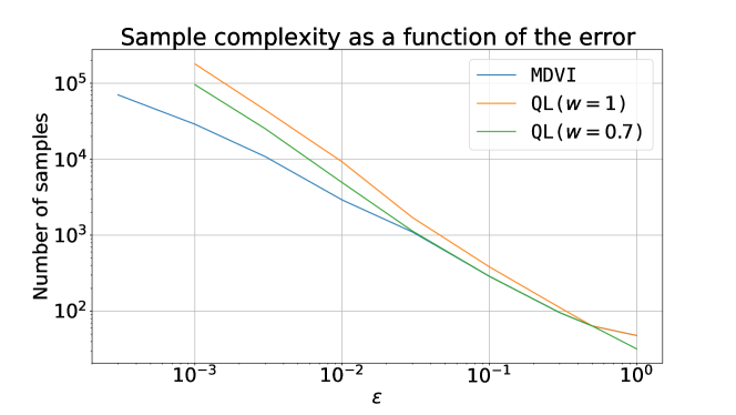
Figure 2: Number of samples needed to reach a certain error.

Influence of $\alpha$.

We showcase the impact of $\alpha$ when $M=1$ in Figure 3. With $\alpha=1$, MDVI will asymptotically converge to $\pi_{*}$. With a $\alpha<1$, MDVI will reach an $\varepsilon$-optimal policy, but will not actually converge to the optimal policy of the MDP (although this $\varepsilon$ can be controlled by choosing a large enough value for $\alpha$, or a larger value of $M$). Indeed, in the latter case, the distance to the optimal policy depends on a moving average of the errors (by a factor $\alpha$). The moving average reduces the variance, but does not bring it zero, contrarily to the exact average implicitly performed when $\alpha=1$. This behaviour is illustrated in Figure 3. We observe there that, with $M=1$, one has to choose a large enough value of $\alpha$ to reach a policy close enough to the optimal one.

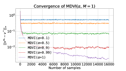
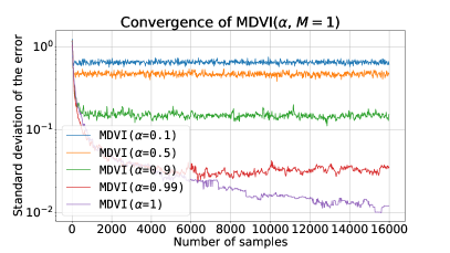
Figure 3: Error of the policy computed by MDVI in function of the number of samples used. Left: mean, Right: standard deviation; estimated over $1000$ MDPs.

Influence of $M$.

Choosing the right $M$ is not that obvious from the theory (it notably depends on an unknown constant $c_{2}$). We illustrate in Figure 4 the influence it has on the speed of convergence of MDVI. We run MDVI with $\alpha=0.99$ (for a setting where $\gamma=0.9$), and for different values of $M$. With a fixed $\alpha$, a larger $M$ allows MDVI to reach a lower asymptotic error, but slows down the learning in early iterations. $M$ cannot however be chosen as large as possible: at one point it start to be useless to increase its value. For instance, moving from $M=5$ to $M=10$ does not allow for a noticeable lower error, but slows the learning. We compare this to the setting where $\alpha=1$ for completeness.

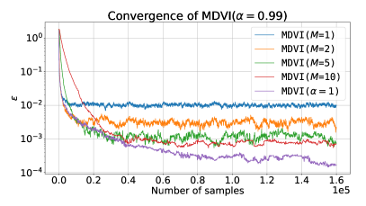
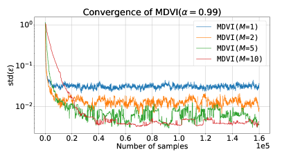
Figure 4: Error of the policy computed by MDVI in function of the number of samples used, for different values of $M$. Left: mean, Right: standard deviation; estimated over $1000$ MDPs. For this value of $\gamma=0.9$, choosing $\alpha=0.99$ matches the condition $\alpha=1-(1-\gamma)^{2}$.

References

- Agarwal et al. (2020) Alekh Agarwal, Sham Kakade, and Lin F. Yang. Model-Based Reinforcement Learning with a Generative Model is Minimax Optimal. In Conference on Learning Theory, 2020.
- Archibald et al. (1995) TW Archibald, KIM McKinnon, and LC Thomas. On the Generation of Markov Decision Processes. Journal of the Operational Research Society, 46(3):354–361, 1995.
- Azar et al. (2011) Mohammad Azar, Mohammad Ghavamzadeh, Hilbert Kappen, and Rémi Munos. Speedy Q-Learning. In Advances in Neural Information Processing Systems, 2011.
- Azar et al. (2013) Mohammad Azar, Rémi Munos, and Hilbert J. Kappen. Minimax PAC bounds on the sample complexity of reinforcement learning with a generative model. Machine Learning, 91(3):325–349, Jun 2013.
- Azar et al. (2017) Mohammad Gheshlaghi Azar, Ian Osband, and Rémi Munos. Minimax Regret Bounds for Reinforcement Learning. In International Conference on Machine Learning, 2017.
- Azuma (1967) Kazuoki Azuma. Weighted sums of certain dependent random variables. Tohoku Mathematical Journal, 19(3):357 – 367, 1967.
- Bernstein (1946) Sergei Natanovich Bernstein. The Theory of Probabilities. Gastehizdat Publishing House, 1946.
- Boucheron et al. (2013) Stéphane Boucheron, Gábor Lugosi, and Pascal Massart. Concentration Inequalities - A Nonasymptotic Theory of Independence. Oxford University Press, 2013.
- Cen et al. (2021) Shicong Cen, Chen Cheng, Yuxin Chen, Yuting Wei, and Yuejie Chi. Fast global convergence of natural policy gradient methods with entropy regularization. Operations Research, 2021.
- Even-Dar et al. (2003) Eyal Even-Dar, Yishay Mansour, and Peter Bartlett. Learning Rates for Q-learning. Journal of Machine Learning Research, 5(1), 2003.
- Fox et al. (2016) Roy Fox, Ari Pakman, and Naftali Tishby. Taming the Noise in Reinforcement Learning via Soft Updates. In Conference on Uncertainty in Artificial Intelligence, 2016.
- Geist et al. (2019) Matthieu Geist, Bruno Scherrer, and Olivier Pietquin. A Theory of Regularized Markov Decision Processes. In International Conference on Machine Learning, 2019.
- Hoeffding (1963) Wassily Hoeffding. Probability Inequalities for Sums of Bounded Random Variables. Journal of the American Statistical Association, 58(301):13–30, 1963.
- Jin et al. (2018) Chi Jin, Zeyuan Allen-Zhu, Sebastien Bubeck, and Michael I. Jordan. Is Q-Learning Provably Efficient? In Advances in Neural Information Processing Systems, 2018.
- Khamaru et al. (2021) Koulik Khamaru, Eric Xia, Martin J Wainwright, and Michael I Jordan. Instance-optimality in optimal value estimation: Adaptivity via variance-reduced Q-learning. arXiv preprint arXiv:2106.14352, 2021.
- Kozuno et al. (2019) Tadashi Kozuno, Eiji Uchibe, and Kenji Doya. Theoretical Analysis of Efficiency and Robustness of Softmax and Gap-Increasing Operators in Reinforcement Learning. In International Conference on Artificial Intelligence and Statistics, 2019.
- Lan (2022) Guanghui Lan. Policy mirror descent for reinforcement learning: Linear convergence, new sampling complexity, and generalized problem classes. Mathematical programming, pp. 1–48, 2022.
- Lattimore & Hutter (2012) Tor Lattimore and Marcus Hutter. PAC Bounds for Discounted MDPs. In International Conference on Algorithmic Learning Theory, 2012.
- Lattimore & Szepesvari (2020) Tor Lattimore and Csaba Szepesvari. Bandit Algorithms. Cambridge University Press, 1st edition, 2020.
- Lee et al. (2018) Kyungjae Lee, Sungjoon Choi, and Songhwai Oh. Sparse Markov decision processes with causal sparse tsallis entropy regularization for reinforcement learning. IEEE Robotics and Automation Letters, 3(3):1466–1473, 2018.
- Li et al. (2020) Gen Li, Yuting Wei, Yuejie Chi, Yuantao Gu, and Yuxin Chen. Breaking the Sample Size Barrier in Model-Based Reinforcement Learning with a Generative Model. In Advances in neural information processing systems, 2020.
- Li et al. (2021a) Gen Li, Changxiao Cai, Yuxin Chen, Yuantao Gu, Yuting Wei, and Yuejie Chi. Is Q-Learning Minimax Optimal? A Tight Sample Complexity Analysis. arXiv preprint arXiv:2102.06548, 2021a.
- Li et al. (2021b) Xiang Li, Wenhao Yang, Zhihua Zhang, and Michael I Jordan. Polyak-Ruppert Averaged Q-Leaning is Statistically Efficient. arXiv preprint arXiv:2112.14582, 2021b.
- Mei et al. (2020) Jincheng Mei, Chenjun Xiao, Csaba Szepesvari, and Dale Schuurmans. On the Global Convergence Rates of Softmax Policy Gradient Methods. In International Conference on Machine Learning, 2020.
- Neu et al. (2017) Gergely Neu, Anders Jonsson, and Vicenç Gómez. A unified view of entropy-regularized Markov decision processes. arXiv preprint arXiv:1705.07798, 2017.
- Scherrer & Lesner (2012) Bruno Scherrer and Boris Lesner. On the Use of Non-Stationary Policies for Stationary Infinite-Horizon Markov Decision Processes. In Advances in Neural Information Processing Systems, 2012.
- Sidford et al. (2018) Aaron Sidford, Mengdi Wang, Xian Wu, Lin Yang, and Yinyu Ye. Near-Optimal Time and Sample Complexities for Solving Markov Decision Processes with a Generative Model. In Advances in Neural Information Processing Systems, 2018.
- Vamplew et al. (2017) Peter Vamplew, Richard Dazeley, and Cameron Foale. Softmax exploration strategies for multiobjective reinforcement learning. Neurocomputing, 263:74–86, 2017.
- Vieillard et al. (2020a) Nino Vieillard, Tadashi Kozuno, Bruno Scherrer, Olivier Pietquin, Remi Munos, and Matthieu Geist. Leverage the Average: an Analysis of KL Regularization in Reinforcement Learning. In Advances in Neural Information Processing Systems, 2020a.
- Vieillard et al. (2020b) Nino Vieillard, Olivier Pietquin, and Matthieu Geist. Munchausen Reinforcement Learning. In Advances in Neural Information Processing Systems, 2020b.
- Wainwright (2019) Martin J Wainwright. Variance-reduced -learning is minimax optimal. arXiv preprint arXiv:1906.04697, 2019.
- Watkins & Dayan (1992) Christopher J. C. H. Watkins and Peter Dayan. Q-Learning. Machine Learning, 8(3):279–292, 1992.
- Yang et al. (2019) Wenhao Yang, Xiang Li, and Zhihua Zhang. A regularized approach to sparse optimal policy in reinforcement learning. In Advances in Neural Information Processing Systems, 2019.
- Zhou et al. (2021) Dongruo Zhou, Quanquan Gu, and Csaba Szepesvari. Nearly Minimax Optimal Reinforcement Learning for Linear Mixture Markov Decision Processes. In Conference on Learning Theory, 2021.