Sub-optimal Approaches to Heteroscedasticity in Silicon Strip Detectors: the Lucky Model and the Super-Lucky Model.

Abstract

The approach to heteroscedasticity of ref. [1] contains a sketchy application of a sub-optimal method of very easy implementation: the lucky model. The supporting proof of this method could not be inserted in [1]. The proof requires the analytical forms of the probability of ref. [2] for the two strip center of gravity. However, those analytical forms suggest also a completion of the lucky-model for the absence of a scaling constant, relevant for combinations of different detector types. The advanced lucky-model (the super-lucky model) can be directly used for track fitting in trackers composed of non-identical detectors. The construction of the weights for the fits is very simple. Simulations of track fitting with this upgraded tool show resolution improvements also for combination of two types of very different detectors, near to the resolutions of the schematic model of reference [1].

Keywords:Center of Gravity; Weighted Average; Probability Density Functions; Position Reconstruction; Micro-strip Detectors; Track Fitting; Least Squares Method; Lucky Model;

1 Introduction

The heteroscedasticity of silicon strip detectors requires a detailed knowledge of the variances of the observations (hits) to insert in weighted least squares to obtain optimal fits [3, 4]. The signals released by a minimum ionizing particle (MIP), if carefully analyzed, allow to extract sub-optimal effective standard deviations defined in ref. [1] as lucky-model. This model was illustrated without a detailed discussion. A more accurate discussion of the lucky model, promised in ref. [1], will be developed here. A brief recall to the equations of ref. [2] is essential for that approximate demonstration. Elements of those equations give a suggestion for the extension of the lucky-model. The lucky model was suggested by a strong similarity of the parameter distributions of the schematic model [5] with the histograms for the two-strip center of gravity (COG₂). This similarity suggested the use of the amplitudes of the histograms directly as weights of homogeneous trackers (formed by identical detectors). These apparently improbable attempts gave results not too different from those of the more complex schematic model. However, the absence of a global scaling factor, intrinsic to the schematic model, imposes a limitation to homogeneous trackers where the expressions of the parameter estimators are invariant under a multiplicative constant. The construction of super-lucky model eliminates this limitation, maintaining the easiness of the approach and a straightforward connection with the data.

2 The COG₂ algorithm

To obtain the PDF for the COG₂ algorithm, we have to define in detail this algorithm. As previously recalled, the signals of three strips must be simultaneously accounted: the strip with the maximum signal (strip $\#\,2$ the seed strip) and the two lateral (strip $\#1$ to the right and strip $\#3$ to the left). Any signal-value in these two strips is accepted, also below the threshold for the insertion of a strip-signal in a cluster by the cluster detection algorithm (as in [10]). Around the strip $\#\,2$, the strip with the maximum signal is selected between the two strips $\#\,1$ and $\#\,3$. Due to the smallest number of strips, this COG₂ has a very favorable signal-to-noise ratio. It is the natural selection for orthogonal incidence on strip detectors with strip widths near to the average lateral drift of the primary charges [8].

2.1 The definition of the COG₂ algorithm

The definition of COG₂ algorithm is condensed in the following equation [6]:

$$x_{g2}=\frac{x_{1}}{x_{1}+x_{2}}\theta(x_{1}-x_{3})-\frac{x_{3}}{x_{3}+x_{2}}\theta(x_{3}-x_{1})\,.$$ (1)

Where $x_{1},\,x_{2},\,x_{3}$ are the random signals in the three strips, and $\theta(z)$ is the Heaviside $\theta$-function ($\theta(x)=0$ for $x\leq 0$ and $\theta(x)=1$ elsewhere). The two $\theta$-functions select the lateral strip with the highest signal. No condition is imposed on the strip $\#\,2$, although it has some constraints for its role of seed strip. This choice eliminates inessential complications and saves the normalization of the PDF.

Our aim is to reproduce the gap for $x_{g_{2}}\approx\,0$, typical of the histograms of COG₂ algorithm. This gap is given by the impossibility (or lower probability) to have $x_{g_{2}}\approx 0$ if the charge drift populates one or both the two lateral strips. The gap grows rapidly with an increase of these two charges. The noise and our selection allow forbidden values.

The $\eta$-algorithm of reference [20] uses a slight different definition. The term $-x_{3}/(x_{2}+x_{3})$ of equation 1 is modified in $x_{2}/(x_{2}+x_{3})$. In this way, the values of $\eta$ are contained in the interval $\{0\vdash\dashv 1\}$, and the gap for $x_{g2}\approx 0$ is spread at the borders of this interval.

The constraints of equation 1, on the three random signal $\{x_{1},x_{2},x_{3}\}$, are inserted in the integral for the PDF of $P_{x_{g2}}(x)$. The integral expression is given by (with the substitution of $x_{g_{2}}$ as $x$):

$$P_{x_{g2}}(x)= \int_{-\infty}^{+\infty}\mathrm{d}\,x_{1}\,\mathrm{d}\,x_{2}\,\mathrm{d}\,x_{3}P_{1}(x_{1})P_{2}(x_{2})P_{3}(x_{3})\Big{[}\delta\big{(}x-\frac{x_{1}}{x_{1}+x_{2}}\big{)}\theta(x_{1}-x_{3})+$$ (2)

$$\delta\big{(}x+\frac{x_{3}}{x_{3}+x_{2}}\big{)}\theta(x_{3}-x_{1})\Big{]}\,.$$

The normalization of $P_{x_{g2}}(x)$ can be immediately proved with a direct $x$-integration. The other integrals are executed with the transformations: $x_{1}=\xi$, $x_{1}+x_{2}=z_{1}$, $x_{3}=\beta$ and $x_{3}+x_{2}=z_{2}$. The jacobian of each couple of transformations is one. The integrals on $z_{1}$ and $z_{2}$ of the two $\delta$-functions can be performed with the standard rules [6]. The general form of $P_{x_{g2}}(x)$ for any type of signal PDF $\{P_{1},P_{2},P_{3}\}$ becomes:

$$P_{x_{g2}}(x)=\frac{1}{x^{2}}\Big{[} \int_{-\infty}^{+\infty}\mathrm{d}\xi P_{1}(\xi)P_{2}(\xi\frac{1-x}{x})|\xi|\int_{-\infty}^{\xi}\mathrm{d}\beta P_{3}(\beta)+$$ (3)

$$\int_{-\infty}^{+\infty}\mathrm{d}\beta P_{3}(\beta)P_{2}(\beta\frac{-1-x}{x})|\beta|\int_{-\infty}^{\beta}\mathrm{d}\xi P_{1}(\xi)\Big{]}\,.$$

Each strip has its own random additive noise uncorrelated with that of any other strip. In strips without MIP signals, the strip noise is well reproduced with Gaussian PDFs. Thus, the PDFs for the signal plus noise of the strip $i$ become:

$$P_{i}(z)=\frac{1}{\sqrt{2\pi}\,\sigma_{i}}\exp[-\frac{(z-a_{i})^{2}}{2\sigma_{i}^{2}}]\ \ \ \ i=1,2,\cdots,n\,.$$ (4)

The Gaussian mean values $\{a_{i}\}$ are the (noiseless) charges collected by the strips and are positive numbers (we assume to have signals from real particles). The parameters $\{\sigma_{i}\}$ are the standard deviations of the additive zero-average Gaussian noise.

The Gaussian PDFs of equation 4, inserted in equation 3, allow the explicit expression of the two integrals on $P_{3}(\beta)$ and $P_{1}(\xi)$ with the appropriate erf-functions. Indicating the remaining integration variable as $z$, equation 3 becomes:

$$P_{xg_{2}}(x)=\frac{1}{2\pi\sigma_{1}\sigma_{2}x^{2}}$$ (5)

$$\Big{(}\int_{-\infty}^{+\infty}\mathrm{d}z\,|z|\Big{\{}\exp\big{[}-\frac{(z-a_{1})^{2}}{2\sigma_{1}^{2}}-\frac{(\frac{(1-x)z}{x}-a_{2})^{2}}{2\sigma_{2}^{2}}\big{]}\,\frac{1}{2}\big{[}1-\mathrm{erf}(\frac{a_{3}-z}{\sqrt{2}\sigma_{3}})\big{]}+$$

$$\frac{\sigma_{1}}{\sigma_{3}}\exp\big{[}-\frac{(z-a_{3})^{2}}{2\sigma_{3}^{2}}-\frac{(\frac{(-1-x)z}{x}-a_{2})^{2}}{2\sigma_{2}^{2}}\big{]}\,\frac{1}{2}[1-\mathrm{erf}(\frac{a_{1}-z}{\sqrt{2}\sigma_{1}})]\Big{\}}\Big{)}\,.$$

The combination of erf-functions and the $|z|$ render impossible an analytical integration of equation 5. The serial development of the erf-function and its successive integration term by term is too cumbersome to be of practical use. (A generalization of the erf-function to the two dimensions is missing). Thus, we have to explore analytical approximations apt to be useful in maximum likelihood search.

2.2 Small |x| approximation

The small $|x|$ approximation is one of the easiest way to handle equation 5. The function $P_{2}(z(1-x)/x)$ can be transformed to approximate a Dirac $\delta$-function for small $|x|$:

$$\frac{\exp\Big{[}-\big{(}\frac{1-x}{x}z-a_{2}\big{)}^{2}\frac{1}{2\sigma_{2}^{2}}\Big{]}}{\sqrt{2\pi}\sigma_{2}}=\frac{\exp\Big{[}-\big{(}\frac{z}{a_{2}}-\frac{x}{1-x}\big{)}^{2}\frac{(1-x)^{2}\,a_{2}^{2}}{2x^{2}\,\sigma_{2}^{2}}\Big{]}}{\Big{(}\frac{\,\sqrt{\,2\,\pi\,}\,\sigma_{2}\,|\,x\,|\,}{\,a_{\,2}\,|\,(1-x)\,|\,}\Big{)}}\frac{|x\,|}{a_{2}|(1-x)|}$$ (6)

$$\approx\frac{|x\,|}{a_{2}|(1-x)|}\delta(\zeta-\frac{x}{1-x})\ \ \ \ \ \ \ \zeta=\frac{z}{a_{2}}\,.$$

The effective standard deviation of the gaussian is $\sigma_{2}|x|/(a_{2}|1-x|)$, this term, for $|x|\rightarrow 0$, allows to identify the gaussian with a Dirac $\delta$-function. The term $|1-x|$ is useful to obtain the combination $a_{1}/(a_{1}+a_{2})$ in the exponent of the Gaussian-like function. A similar transformation can be applied to $P_{2}(z(-1-x)/x)$, the integration on $\zeta$ is now immediate and the small $|x|$ probability $P_{xg_{2}}$ becomes [6]:

$$P_{xg_{2}}(x)= \frac{|a_{2}|}{2\sqrt{2\pi}}\Big{\{}\frac{\exp\big{[}-(x-\frac{a_{1}}{a_{1}+a_{2}})^{2}\frac{(a_{1}+a_{2})^{2}}{2(\sigma_{1}^{2}(1-x)^{2})}\big{]}\big{(}1-\mathrm{erf}\big{[}(\frac{a_{3}}{a_{3}+a_{2}}-x)\frac{a_{2}+a_{3}}{\sqrt{2}(1-x)\sigma_{3}}\big{]}\big{)}}{\sigma_{1}(1-x)^{2}}+$$ (7)

$$\frac{\exp\big{[}-(x+\frac{a_{3}}{a_{3}+a_{2}})^{2}\frac{(a_{3}+a_{2})^{2}}{2(\sigma_{3}^{2}(1+x)^{2})}\big{]}\big{(}1-\mathrm{erf}\big{[}(\frac{a_{1}}{a_{1}+a_{2}}+x)\frac{a_{1}+a_{2}}{\sqrt{2}(1+x)\sigma_{1}}\big{]}\big{)}}{\sigma_{3}\,(1+x)^{2}}\Big{\}}\,.$$

The term $a_{2}$ is a positive constant (the noiseless charge of the seed strip) and the absolute value can be eliminated, but for future developments is better to remember its presence. Two different simulated distributions are reported in [5, 6] and compared with equation 7, the first one did not contain the Landau fluctuations, the second one contains approximate Landau fluctuations. At orthogonal incidence, the Landau fluctuations are well described by the fluctuations of the total collected charges.

The approximation of equation 7 reproduces, in a reasonable way, the COG₂ PDF also for non small $x$. In fact, the real useful range of $x$ is $|x|\leq 0.5$, and the factor that is supposed small is $|x|\sigma_{2}/a_{2}$. But, the constant $a_{2}$ is connected to seed of the cluster and it has a high probability to be larger than few times $\sigma_{2}$. The $a_{2}$ noisy detected part, $x_{2}$, must assure a reasonable detection efficiency of the hit. Surely equation 7 becomes useless around $x=\pm 1$. In any case, better approximations are always useful, given that the probability $P_{xg_{2}}(x)$ has to apply to a large set of experimental configurations. A conceptual incompleteness of equation 7 is the lack of the normalization. The normalization assures a constant probability of the impact point, but its lack is not a real limitation for the practical use of equation 7.

2.3 A better approximation for $P_{xg_{2}}(x)$

A more accurate approximation for $P_{xg_{2}}(x)$ can be obtained retaining the small $x$ approximation for the two $\mathrm{erf}$-function of equation 5 and integrating on $z$ the remaining parts [11]. Now the two integrals have analytical forms calculated in ref. [2]. This approximation saves also the normalization.

$$P_{xg_{2}}(x)= \Big{\{}\frac{\Big{|}a_{2}(1-x)\sigma_{1}^{2}+a_{1}x\sigma_{2}^{2}\Big{|}}{2\sqrt{2\pi}[(1-x)^{2}\sigma_{1}^{2}+x^{2}\sigma_{2}^{2}]^{3/2}}\exp\big{[}-(\frac{a_{1}}{a_{1}+a_{2}}-x)^{2}\frac{(a_{1}+a_{2})^{2}}{2(\sigma_{1}^{2}(1-x)^{2}+x^{2}\sigma_{2}^{2})}\big{]}\Big{\}}$$ (8)

$$\Big{\{}1-\mathrm{erf}\big{[}(\frac{a_{3}}{a_{3}+a_{2}}-x)\frac{a_{2}+a_{3}}{\sqrt{2}(1-x)\sigma_{3}}\big{]}\Big{\}}+\ \ a_{1}\leftrightarrow a_{3},\ \sigma_{1}\leftrightarrow\sigma_{3},\ \ x\rightarrow-x\,.$$

Although equation 8 represents a better approximation compared to equation 7, some discrepancies remain in very special configurations. These discrepancies are absent, or heavily reduced, in the longer approximation reported at the end of ref. [2]. However, for our necessity this approximation suffices.

3 The lucky model

A set of simulations highlight some peculiar properties of the PDF of equation 8. The effective use of equation 8 in track reconstruction, and similarly for all the other PDFs, requires the completion with the functional dependence from the hit impact point. The method for this completion is discussed in [5] with the construction of the functions $a_{j}(\varepsilon)$. Differently from their definition in the previous equations, the $a_{j}(\varepsilon)$ of [5] are constructed normalized to one. For tuning them to each hit, the parameter $E_{0}$ scales the $a_{j}$ to the appropriate values; $E_{0}$ is the noiseless total charge collected by the three strips of each hit. The functions $a_{j}(\varepsilon)$ are obtained by large averages of hit positioning given by the $\eta$-algorithm [8]. The data of the test-beam [22] were used for those constructions. The unbiasedness of the $\eta$-algorithm and the special averages [5] give to the $a_{j}$ realistic functional dependencies from the hit impact point $\varepsilon$. The finiteness of the averages leave small artifacts, but they have no detectable effects on the distributions of the fitted parameters.

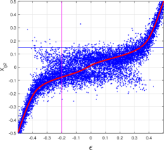
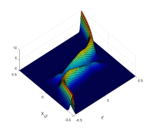
Figure 1: Left side. Scatter-plot of a sample of simulated $x_{g2}$ data in function of the impact point $\varepsilon$, the red line is the $\eta$-algorithm. The magenta line and the blue line are for the following figures. The right side is a 2D illustration of the PDF for $x_{g2}$ in function of the impact point $\varepsilon$ for $E_{0}=150$ ADC counts.

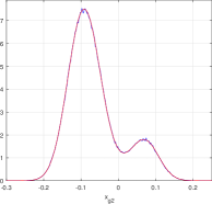
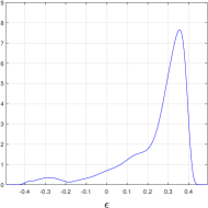
Figure 2: Left side: Empirical PDFs of $x_{g_{2}}$ (blue line) compared with equation 8 (red line) for a model of silicon detector [5] for an impact point $\varepsilon=-0.2$, all the $\sigma=8$ ADC counts, and $a_{1}=0.01\,E_{0}$, $a_{2}=0.91\,E_{0}$ and $a_{3}=0.08\,E_{0}$ are the charges collected by the three strips, here $E_{0}$, the total charge of the three strips, is 150 ADC counts (the magenta line of figure 1). The right side is the probability distribution for $x_{g2}=0.15$, the blue line in the scatter-plot of figure 1

A simple simulation can be used to verify the consistency of equation 8 and to illustrate the weak gap present in a distribution of simulated $x_{g_{2}}$ in the scatter-plot of figure 1. The data of the simulation are generated with the function randn of MATLAB [12] and with the equations $x_{i}=\sigma_{1}$ randn(1,N)$+a_{i}*E_{0}$, and inserted in equation 1 to calculate a large sample of $x_{g2}$. Values for $a_{i}$ ($a_{1}=0.01$, $a_{2}=0.91$, $a_{3}=0.08$, $E_{0}=150$ ADC counts and $\sigma_{1}=8$ ADC counts), $\sigma_{i}$ are extracted from [5] for orthogonal incidence on the two types of silicon detectors studied there. The type of detector considered in figures 1 and 2 is of normal type with a high noise of 8 ADC counts, one of the two types studied in [5, 6]. To simplify the simulations, all the $\sigma_{i}$ are identical to the most probable noise of the strips. The noisy strips are very few, and it is an useless complication to explore different $\sigma_{i}$. The left side of figure 2 reports the overlaps of the analytical PDF and the PDF obtained from the simulated data. The probability decrease between the principal and secondary maximum of figure 2, originating a similar reduction along the magenta line in the scatter-plot of figure 1. The secondary maximum is produced by the noise that promotes the minority noiseless signal to becomes the greater one. Signal clusters with lower total charge show larger gaps.

The right side of figure 2 shows the probability distribution of the hit impact points for a given value of the two strip COG $x_{g2}$. The $x_{g2}=0.15$ is the constant value of $x_{g2}$, the blue line in the scatter-plot of figure 1. The integral of this distribution gives the probability for this value of $x_{g2}$ for 150 ADC counts. We limit the integration to a two strip length centered to the maximum of the distribution. In this way, the histogram of $x_{g2}$ is analytically reconstructed and reproduces well the histogram of the simulated data [5]. Products of probability distributions, similar to that of figure 2, are used to find the maximum likelihood of a set of hits for a track. This figure shows also the presence of outliers in the tail of the distribution. These outliers are difficult to handle because they are masked as good hits in the schematic model. Instead the maximum likelihood is able to avoid their disturbances in the fits. In [5], we illustrate one of the worst outlier and how the maximum likelihood find almost exact parameters of the fitted track. We accumulated many similar simulated events with excellent maximum likelihood reconstructions and worst schematic model and standard fit reconstructions.

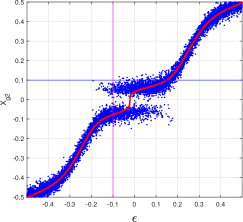
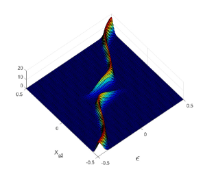
Figure 3: Similar to figure 1 for floating strip detectors. Left side. Scatter-plot of $x_{g2}$ data in function of $\varepsilon$. The right side. 2D PDF for $x_{g2}$ in function $\varepsilon$.

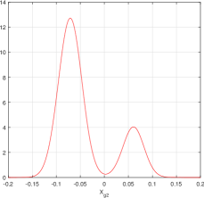
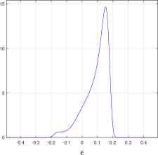
Figure 4: Floating strip detector. Left side: analytical PDFs of $x_{g_{2}}$ for $\varepsilon=-0.1$ and E${}_{0}=150$ ADC counts. Right side: the probability distribution for $x_{g2}=0.1$, the blue line in the scatter-plot of figure 3

Plots similar to figure 1 can be produced for the floating strip detector [5, 22]. The plots illustrate the large differences of this excellent detector type with very low noise and the floating strips, able to distribute the incoming signal to the nearby strips. The gap for COG${}_{2}\approx\,0$ is a real gap without data in a scatter-plot with a moderate number of events. The effects of the low noise (4 ADC) are quite evident in all the distributions.

3.1 A demonstration of the lucky model

The availability of the analytical equations for the COG PDFs allows a direct discussion of the lucky model [1]. The structure of [1] had to be heavily deviated from its aims to complete this discussion. As sketchily illustrated in [1], this sub-optimal model is suggested by the similarity of the trends of the effective standard deviations for the schematic model and the trends of the $x_{g2}$ histograms (similarly for the COG₃ histograms). Those effective standard deviations were obtained from the variances of functions of $\varepsilon$, two of them illustrated in the right side of figure 2 and figure 4, as explained in [5, 6]. The scatter-plots of these effective standard deviations clearly show the trends of the $x_{g2}$ histograms. In [5], we gave an approximate motivation of this non obvious correlation. We can complete those motivations with more details. The reasoning of [5] suppose (as always) an uniform population of events on a strip; thus, for regions with large effective variances, a relative larger fraction of events ends up to the corresponding $x_{g2}$-values. Instead, for small effective variances, a relative lower fraction of events ends up to these $x_{g2}$-values. Assuming the correctness of this explanation, a test of its effectiveness in improving a fit is a natural output. Although the result of this "lucky" test of [1] was successful, a detailed supporting proof is essential for a confident use. This proof was a pledge of reference [1]. However, the construction of this proof requires an analysis of equation 8 and the left sides of figures 2 and 4, tools not available in [1].

Equation 8 shows the $P_{xg_{2}}(x)$ as formed by two bumps (approximatively Gaussian) whose maxima follows the noiseless function $x_{g2}(\varepsilon)$. Beyond the center of the strip, the last part of each bump decreases rapidly as illustrated in the 2D PDF of figure 1 and figure 3. As discussed in [8], the $\eta$-algorithm produces functions that show strong similarity with the noiseless $x_{g2}(\varepsilon)$, in the relevant parts of the two bumps. Therefore, we can use the functions $x_{g2}(\eta)$, of the $\eta$-algorithm, in place of the exact noiseless $x_{g2}(\varepsilon)$, and to follow the path of the bump maxima and two corresponding positions at the half-maximum. The distance between these two positions is the full-width-at-half-maximum of the $P_{xg_{2}}(x)$ in the direction of the hit impact point. Each one of these two points follow paths parallel to the noiseless $x_{g2}(\varepsilon)$ one above and the other below the path followed by the bump maximum. Again, we approximate these paths with the $x_{g2}(\eta)$-function. The two sides of figure 5(out of scale for a better illustration) report these paths for the two types of detectors of [5, 6]. The vertical segments are the full-width-at-half-maximum of $P_{xg_{2}}(x)$ and will be defined as $\sigma_{x_{g2}}$. The positioning errors $\sigma_{\eta}$ of a generic $x_{g2}^{0}$, possible realizations of their COG₂, are the horizontal black lines. The amplitudes of the horizontal segments are the positioning errors relevant for the weighted least squares.

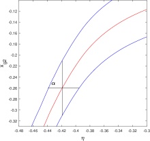
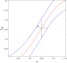
Figure 5: Relation of the amplitude of the $x_{g2}$ error of equation 8 with the positioning error of a given value of COG₂ due to an observation. Left side: normal strip detector. Right side: floating strip detector

The blue lines are curved lines and only approximatively describe a triangle, the ratio of $\sigma_{x_{g2}}$ and $\sigma_{\eta}$ can be estimated as:

$$\tan(\alpha)\approx\frac{\sigma_{x_{g2}}}{\sigma_{\eta}}\ \ \ \ \frac{1}{\tan(\alpha)}=\frac{\mathrm{d}\,\eta}{\mathrm{d}\,x_{g2}}\big{|}_{x_{g2}^{0}}=\Gamma(x_{g2}^{0})\ \ \ \ \ \sigma_{\eta}\approx\frac{\sigma_{x_{g2}}}{\tan(\alpha)}=\sigma_{x_{g2}}\,\Gamma(x_{g2}^{0})$$ (9)

where $\Gamma(x_{g2}^{0})$ is the amplitude of the normalized histogram of COG₂ for the value $x_{g2}^{0}$. In fact, the starting point of the $\eta$-algorithm of [8] is the differential equation ${\mathrm{d}\,\eta}/{\mathrm{d}\,x_{g2}}=\Gamma(x_{g2})$. Neglecting the differences of $\sigma_{x_{g2}}$, the $\eta$-algorithm gives all the elements for a good fit; the corrections of the COG₂ systematic errors and the weight for track fitting in an array of identical detector layers. In this case, the expressions of the parameter estimators of the fit are independent from the (assumed) constant $\sigma_{x_{g2}}$. Therefore, the values of $\Gamma(x_{g2})$ can be used directly as weights of the observations in a weighted least squares of a track.

In presence of large data gaps (i.e. absence of data) in the histogram of COG₂, the function $x_{g2}(\eta)$ acquires discontinuities that complicate the plots of figure 5, as discussed in [9]. In any case, the presence of large gaps in the COG histograms should be avoided for the excessive loss of information. It is better the use of COG-algorithms with more strips.

3.2 Advanced form for the lucky model: The super-lucky model

The precedent discussion is a justification of the simple lucky model of [1]. We utilized this model with a set of identical detectors, inserting directly the amplitudes of the COG₂ histograms in place of effective standard deviations of the observations. The scaling factor ($\sigma(x_{g2})=$constant) of the this approximate guess is simultaneously present in the numerator and in the denominator of the expressions of the fitted parameters and it simplifies. This simplification is impossible for arrays with detectors of different type. Hence, the (assumed) constant vales of the scaling factors ($\sigma_{x_{g2}}$) become relevant to tuning the amplitudes of different histograms with the properties of the different detectors. The full calculation of some effective standard deviations of the schematic model looks unavoidable. However, the demonstration of equation 9 recalls the attention to the possible variations of $\sigma_{x_{g2}}$. We supposed that the principal bumps of equation 8 are very near to Gaussian PDFs. We can push this assumption forward and extract from equation 8 approximate forms for $\sigma_{x_{g2}}$ (abandoning the full-width-at-half-maximum in favor of the usual standard deviation):

$$\sigma_{x_{g2}}^{R}=\frac{\sqrt{\sigma_{1}^{2}(1-|X^{R}|)^{2}+\sigma_{2}^{2}\,(X^{R})^{2}}}{a_{1}+a_{2}}\ \ \ \ \ X^{R}=\frac{a_{1}}{a_{1}+a_{2}}$$ (10)

$$\sigma_{x_{g2}}^{L}=\frac{\sqrt{\sigma_{3}^{2}(1-|X^{L}|)^{2}+\sigma_{2}^{2}\,(X^{L})^{2}}}{a_{3}+a_{2}}\ \ \ \ \ X^{L}=-\frac{a_{3}}{a_{3}+a_{2}}$$

The substitutions of $X^{R}$ and $X^{L}$, systematically in equation 8, transform the two bumps in two Gaussian PDFs. In any case, also these approximate forms are outside our reach, $a_{1}$, $a_{2}$ and $a_{3}$ are the noiseless signals released by the MIP. Instead, we have their noisy version. Similarly for $X^{R}$ and $X^{L}$ that are the noiseless COG₂, ratio of noiseless signals. The only well defined parameters are $\sigma_{1}$, $\sigma_{2}$ and $\sigma_{3}$, the strip noises, calculated at the initialization stage of the strip detectors. However, we can try to combine the noisy data to see what happen (we were lucky with the COG₂ histogram in [1]). The COG₂ algorithm is described in equation 1 with the definition of $x_{g2}$, therefore, the approximate (super-lucky) $\Sigma_{sup}$ could be:

$$\Sigma_{sup}=\frac{\sqrt{\sigma_{1}^{2}(1-|x^{R}|)^{2}+\sigma_{2}^{2}\,(x^{R})^{2}}}{x_{1}+x_{2}}\,\theta(x_{1}-x_{3})+\frac{\sqrt{\sigma_{3}^{2}(1-|x^{L}|)^{2}+\sigma_{2}^{2}\,(x^{L})^{2}}}{x_{3}+x_{2}}\,\theta(x_{3}-x_{1})$$ (11)

$$x^{R}=\frac{x_{1}}{x_{1}+x_{2}}\ \ \ \ \ \ \ \ \ x^{L}=-\frac{x_{3}}{x_{3}+x_{2}}\ \ \ \ \ \ \ \ \ \ \ \ \ \ \ \ \sigma_{\eta}=\Sigma_{sup}(x_{g2})\,\Gamma(x_{g2})$$

The insertion of equation 11 in the calculation of the effective standard deviations of the observation can be compared with those of the schematic model for the two widely different detector types of our simulations. We tested also the use of the soft cut-offs with the erf-functions of equation 8 in place of the sharp cut-offs of equation 11, but this insertion adds complications without any visible effect on the simulations.

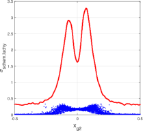
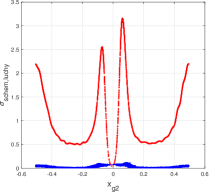
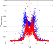
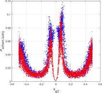
Figure 6: Upper plots: Blue dots: schematic model, Red dots COG₂ histograms. left side plot: normal strip detector. Right side plot: floating strip detector. Lower Plots: Blue dots: schematic model, Red dots $\sigma_{\eta}(x_{g2})$ of equation 11. left side plot: normal strip detector. Right side plot: floating strip detector

The upper plots of figure 6 illustrates the relations of the effective standard deviations of [5, 6] for the two schematic models and the corresponding amplitudes of the lucky-model. The lower plots of figure 6 show the (surprising) good overlaps of the guessed weights of equation 11 for the advanced lucky-model (hereafter super-lucky model) with the two schematic models of [5, 6]. Also the limitation to an identical set of detectors is solved by the super-lucky model.

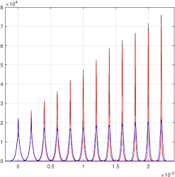
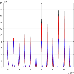
Figure 7: Comparison of the schematic model (black lines), the super-lucky-model (red lines) and the standard model (blue lines) for the track direction reconstructions with 2, 3 $\cdots$, 13 detectors layers. Left side plot: normal strip detectors, right side plot: floating strip detectors

Figure 7 shows the quality of the track reconstructions produced by the super-lucky model that is very near to the schematic model, substantially better than the simple lucky model (not reported in figure for a better readability). Similarly to [1], figure 7 reports the empirical PDFs for the fitted directions of 150,000 straight tracks at orthogonal incidence on a set of parallel and equidistant detector layers. To clearly observe the differences of the parameter distributions, the first distributions with two detector layers are centered on zero (as it must be) the other distributions with N=3, N=4, $\cdots$, up to N=13 are shifted by N-2 identical steps. We start always from two detector layers as a check of the methods, all of them must coincide.

An interesting comparison is the relations of the maxima of the distributions of figure 7 and the standard deviations of those distributions. We have to recall the possible complications with the standard deviation for systems with PDFs having tails similar the Cauchy-Agnesi PDFs. As in ref. [4, 1] we report $1/\sqrt{2\,\pi\,S_{d}^{2}}$ where $S_{d}$ is the standard deviation of one of the distributions in figure 7. For Gaussian PDF this ratio coincides with the maximum of the PDF. As expected by the (Cauchy-Agnesi) tails of the PDFs, we observe in these plots large distances from the maxima. The maxima of the standard least squares are the nearest.

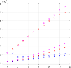
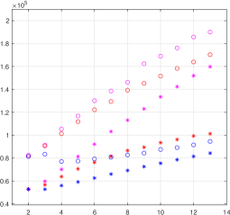
Figure 8: Comparisons of maxima and $1/\sqrt{2\,\pi\,S_{d}^{2}}$, $S_{d}$ the standard deviation of one of the three distributions. The magenta color refers to the schematic model, the red color for the super-lucky model and the blue color for the standard fit. The circles indicated the maxima and the asterisks are for ratio of the standard deviations. The left plot is for the normal strip case. The right plot is for the floating strips detectors.

The results of the lucky model is not reported to avoid an excessive complication in the plots However, the simulations with the lucky model for normal strip detector are reported in ref. [1]. The results of the lucky model for the floating strip detector are appreciably lower ($\approx 12\%$) than the results of the super-lucky model.

3.3 The super-lucky model for the combination of two very different detector types

The super-lucky model was studied just for the application of the lucky model to trackers with different types of detector layers. Thus, we simulate a set of trackers starting with two detector layers, one for each type, and adding alternating a floating strip detector and a normal detector. Figures 7 and 8 show the large differences in resolution of these two types of detectors composing this new system; the floating strip detectors with a low noise of four ADC counts and the normal detectors with a noise of eight ADC counts. The floating strips add further improvement in resolution for their spreading the signal in the nearby strips.

The left sides of figures 9 and 10 illustrate the similarity in resolution of the super-lucky model and the schematic model for this non-homogeneous set of trackers. For comparison, in the right sides of figures 9 and 10, we report also the simulation with the simpler lucky model. The improvements of the super-lucky model are evident. Despite of its inconsistency in this case, the simpler lucky model shows a substantial increase of resolution compared with the standard least-square. The rough pieces of information, contained in the model, are able to enrich the parameter distributions of exact values. Instead, the standard deviations of the parameters of this simpler model are very near (although better) to those of the standard least-squares, signaling large tails given by tracks without good hits. The super-lucky model has standard deviations appreciably better than the lucky-model, thus the added corrections 11 recover part of the tails. However, the effects due to the large tails of the distributions can be attenuated by the selection of tracks with two or more good hits.

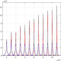
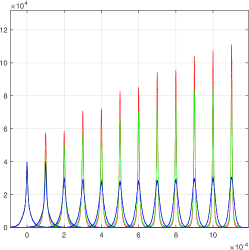
Figure 9: Left plot: Comparison of the schematic model (black lines), super-lucky-model (red lines) and the standard model (blue lines) for the track direction reconstructions half detector layers of floating strip detector and half with normal detector layers. Left side plot: always half and half detector types, the green lines are given by the simpler lucky model, the other lines are those of the right plot.

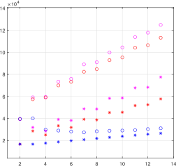
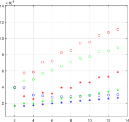
Figure 10: Mixed detector quality. Comparison of maxima and $1/\sqrt{2\,\pi\,S_{d}^{2}}$, $SD$ the standard deviation of one of the three distributions. The magenta color refers to the schematic model, the red color for the super-lucky model and the blue color for the standard fit. The circles indicated the maxima and the asterisks are for ratio of the standard deviations. The left plot is for the normal strip case. The right plot is for the comparison with the simpler lucky model (green color).

In this set of trackers, the growth of the maxima are dominated by the floating strip detectors, the addition of a layer of this type of detectors shows an evident increase of the maxima of the distributions. Instead, the addition of a layer of normal detectors has a negligible effect. The usual linear growth of the two figures 8 becomes the step like growth of figure 9 and figure 10. Also the standard least-square fit shows a drastic reduction of the maxima and a general deterioration compared to the simpler analysis of the parts with good detector types. All the other models show improvements also for the addition of low quality detectors. In [4], the resolutions for these non-Gaussian distributions are defined by the maxima of the distributions: The higher the maximum the better the resolution. The method of fitting a Gaussian in the core of the distributions (as for example in [14, 21]) gives too high values for these very narrow distributions. The demonstrations of [3] and [4] proves that the standard least squares model is never optimum outside the homoscedastic systems. The results of the previous two suboptimal models enforce the power of those demonstrations. In fact, any deviation from homoscedasticity, also with weak correlations with the true variances for the observations, is able to improve the fit resolution beyond the results of the standard least squares.

All these results are exclusively obtained with the hit position given by the $\eta$-algorithm as shown in the two sides of figure 5. The use of the positions given by the COG₂-algorithm (as often done) suppresses totaly the goodness of these results and the parameter distributions are lower than those of the standard least-squares fits (even these substantially lower than those given by the $\eta$-algorithm).

3.4 Further discussions and comparisons for the simulations and data

For an happy coincidence we found a very effective approximation of the schematic model. When we started to write equation 9, we have no idea of those further upgrading. They come out from the environment in which we are writing the equation. Surprising enough were the overlaps among the effective standard deviations for excellent hits, illustrated in the low part of figure 6. Further checks showed also that the differences of these parameters, for the same hit, are around $\approx 10\%,\,20\%$ for many thousands of excellent hits. A very improbable random event, thus a mathematical explanation has to be found. We have to recall that the construction of the effective variances in the schematic model contains an arbitrariness to be fixed. Equation 11 of [6] reports a detailed description of this construction. The probability distributions in the integrals are similar to those at the right side of figures 2 and 4, very different from Gaussian PDFs for the COG₂ around zero. Instead, in the regions of excellent hits for the floating strip detectors, the simulations show strong similarity with Gaussian PDFs for the core of the distributions. The tails are surely different (Cauchy-Agnesi type) and had to be cut to avoid divergences. The effective variances showed a sensible dependency from the cut position. Our decision about the cut was essentially "aesthetical", the effective variances had to reproduce the core with Gaussian PDFs for a small number (four or five) of excellent hits where that core was very similar to a Gaussian. At the same time, the systematic comparison of the real PDFs with Gaussian PDFs gives indications of deviations from optimality. In fact, the Gaussian PDFs are the optimum for the schematic model. Evidently this selection produces effective standard deviations very near to those of the super-lucky model almost perfect for excellent hits. This type of hits turned out to be far more numerous [5] than our best expectation.

In any case, a different selection of the cuts can change this convergence and perhaps the fit quality for the loss of optimality for those excellent hits. At the moment of these selections we were in a very early stage of the work, with no idea of the results.

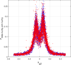
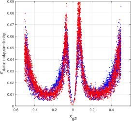
Figure 11: Blue dots: $\sigma_{\eta}(x_{g2})$ of equation 11 obtained from the data of a test beam [22], Red dots $\sigma_{\eta}(x_{g2})$ of equation 11 from simulations. Left side plot: normal strip detector. Right side plot: floating strip detector

Other interesting comparisons are possible: the $\sigma_{\eta}(x_{g2})$ of the lucky model from our simulations and the data. The calculation of these expressions are very fast (contrary to the schematic model that requires a huge number of numerical integrations). Figure 11 shows these comparisons for the two types of detectors. The blue dots are now the $\sigma_{\eta}(x_{g2})$ of the super-lucky model given by the data from a test-beam [22] and the red ones are those of the low side of figure 6. The overlaps are excellent, showing the high quality of our method of simulation [5]. Although, the histograms of the simulated signal distributions on the strips show excellent overlaps with those from data, this type of comparison was never explored before for evident reasons. The $\sigma_{\eta}(x_{g2})$-values have a non trivial relation with the data and these strict correlations enforce our system of extracting/defining [5] the average signal distribution on the strips.

It is reasonable to expect that the use of the $\sigma_{\eta}(x_{g2})$-values, in real track fitting, give results comparable to those of figures 7 and 8 for that detector types or combinations (figures 9 and 10).

4 Conclusions

The analytical expressions for the two strip center of gravity allow an explanation of the a suboptimal handling of the heteroscedasticity for silicon micro-strip detector: the lucky model. This explanation open the way to an advanced form; the super-lucky model. This advanced form is able to extend the lucky model to trackers composed by detectors with very different properties. The reported simulations show a substantial increase of the parameter resolution of the super-lucky model, well beyond the results of the standard least squares and very near to those of the schematic model. This method, for the easy availability of its composing elements, adds negligible complications to the fitting work with substantial increases of resolution.

References

- [1] Landi G.; Landi G. E. Beyond the -limit of the least squares resolution and the lucky-model Instruments 2022, 6, 10. https://doi.org/10.3390/ instruments6010010
- [2] Probability Distributions of Positioning Errors for Some Forms of the Center of Gravity Algorithm. arXiv:2004.08975[physics.ins-det] https://arxiv.org/abs/2004.08975
- [3] Landi G.; Landi G. E. The Cramer-Rao inequality to improve the resolution of the standard least-squares method in track fitting. Instruments 2020, 4, 2. https://doi.org/10.3390/instruments4010002
- [4] Landi G.; Landi G. E. Generalized Inequalities to Optimize the Fitting Method for Track Reconstruction. Physics 2020, 2, 608-623. https://doi.org/10.3390/physics2040035
- [5] Landi G.; Landi G. E. Improvement of track reconstruction with well tuned probability distributions JINST 9 2014 P10006. arXiv:1404.1968[physics.ins-det] https://arxiv.org/abs/1404.1968
- [6] Landi, G.; Landi G. E. Optimizing momentum resolution with a new fitting method for silicon-strip detectors INSTRUMENTS 2018, 2, 22
- [7] Devore, J.L.; Berk, K.N. Modern Mathematical Statistics with Applications; Springer: New York, NY, USA, 2018.
- [8] G. Landi, Problems of position reconstruction in silicon microstrip detectors Nucl. Instr. and Meth. A 554 (2005) 226.
- [9] G. Landi, The center of gravity as an algorithm for position measurements Nucl. Instr. and Meth. A 485 (2002) 698 arXiv:1908.04447 [physics.ins-det] https://arxiv.org/abs/1910.04447.
- [10] Landi G., Landi G. E. Silicon Microstrip Detectors Encyclopedia 2021, 1, 1076-1083. https://doi.org/10.3390/encyclopedia1040082.
- [11] MATHEMATICA 6 Wolfram Inc. Champaign IL, USA
- [12] MATLAB 2020 The MathWork Inc. Natic, MA, USA
- [13] F. Hartmann, Silicon tracking detectors in high-energy physics Nucl. Instrum. and Meth. A 666 (2012) 25
- [14] The CMS Collaboration, The performance of the muon detector in proton-proton collision at TeV at LHC J.Instrum. 8 (2013) P11002 (arXiv.1306.6905)
- [15] B. V. Gnedenko The Theory of Probability and Elements of Statistics (AMS Chelsea Publishing -Providence Rhode Island )
- [16] Gauss C.F., Méthode des Moindres Carrés. Mémoires sur la Combination des Observations. Franch translation by J. Bertrand; revised by the author; Mallet-Bachelier Paris. France 1855 . Available online: (accessed on 1 September 2018).
- [17] The CMS Collaboration, Description and Performance of track and primary vertex reconstruction with the CMS tracker. 2014 JINST 9 P10009
- [18] V.V. Samedov Inaccuracy of coordinate determined by several detectors’ signals 2012 JINST 7 C06002
- [19] Landi G., Landi G. E., Positioning Error Probabilities for Some Forms of Center-of-Gravity Algorithm Calculated with the Cumulative Distributions. Part II. arXiv:2103.03464 [physics.ins-det] https://arxiv.org/abs/2103.03464
- [20] Belau, E.; Klanner, R.; Lutz, G.; Neugebauer, E.; Seebrunner, H.J.; Wylie, A. Charge collection in silicon strip detector. Nucl. Instrum. Methods Phys. Res. A 1983, 214, 253-260.
- [21] Sirunyan, A.M.; The CMS Collaboration. Performance of the reconstruction and identification of high-momentum muons in proton proton collision at = 13 TeV. J. Instrum. 2020, 15, P02027
- [22] Adriani, O.; Bongi, M.; Bonechi, L.; Bottai, S.; Castellini, G.; Fedele, D.; Grandi, M.; Landi, G.; Papini, P.; Ricciarini, S.; et al. In-flight performance of the PAMELA magnetic spectrometer. In Proceedings of the 16th International Workshop on Vertex Detectors, (PoS(Vertex 2007)048), Lake Placid, NY, USA, 23-28 September 2007.